ohi oz ©ptiba $ap~s - nasa · bfs®8 ©ptiba $ap~s 2018-04-25t03:15:54+00:00z. optimal inputs for...
TRANSCRIPT

by
OZ
U'J)
P.qC
OHI
(ul+
n I
C) I
ot0
Lnn
UcF
-_
Department of Aeronautics and Astronautics
May 1972
SUDAAR NO. 440
Iteproduced C ANATIONAL TEC' FllC. 'l:,IINFORMATIOSERYICE';
This research was sponsored by theNATIONAL AERONAUTICS AND SPACE ADMINISTRATION
under Research Grants:NASA NG R 05-020-526,NASA NGL 05-020-007
I -.
OMSER I© $ME 78A$ IR$NABBH
BFs®8©ptiBa $ap~S
https://ntrs.nasa.gov/search.jsp?R=19720024607 2018-06-20T15:30:22+00:00Z

OPTIMAL INPUTS FOR SYSTEM IDENTIFICATION
by
Donald B. Reid
Department of Aeronautics and AstronauticsGuidance and Control Laboratory
STANFORD UNIVERSITYStanford, California 94305
This research was sponsored by theNATIONAL AERONAUTICS AND SPACE ADMINISTRATION
under Research Grants:
NASA NGR 05-020-526,NASA NGL 05-020-007
SUDAAR NO. 440
May 1972

PRECEDING PAGE BLANK NOT FILMED
ABSTRACT
This thesis is concerned with determining optimal inputs to identify
parameters of linear dynamic systems. Identification criteria are
presented for linear dynamic systems with and without process noise.
With process noise, the state equations are replaced by the Kalman filter
equations. If the identification performance index is expanded in a
Taylor's series with respect to the parameters to be identified, then
maximizing the weighting factor of the quadratic term with respect to
the inputs will insure that an identification algorithm will converge
more rapidly and to a more accurate result than with non-optimal inputs.
The expectation of this weighting factor is known as the Fisher informa-
tion matrix, and its inverse is a lower bound for the covariance of the
parameters. Direct and indirect methods of calculating the information
matrix are presented for systems with and without process noise. The
input design criterion used is the trace of the inverse of the informa-
tion matrix. Minimizing this criterion appears to have some advantages
over maximizing the trace of the information matrix;
With amplitude constraints on the input, the optimal input is full
on in one direction or full on in the other direction (bang-bang). A
gradient method is then used to minimize with respect to the switch
times. The method is then applied to some simple illustrative examples.
For sufficiently long tests, the optimal switch times are equally spaced
and may be computed using the first few terms of the Fourier series for
a square wave, minimizing with respect to the fundamental frequency.
For reasonable amounts of deterministic input, the overall effect of
process noise is to decrease the identification accuracy.
The method is then applied to finding the optimal elevator deflec-
tion to identify two damping derivatives of the short period longitudinal
Preceding page blank -iii-

equations of motion of an airplane. A simulation verifies the improve-
ments of the optimal input over non-optimal inputs. Preliminary results
are also obtained using the method to find the optimal aileron and
rudder inputs to identify four damping derivatives of the lateral equa-
tions of motion of an airplane.
-iv-

ACKNOWLEDGMENTS
I wish to thank my advisor, Professor Arthur E. Bryson, Jr.,
for his support and encouragement during the course of this research.
I also wish to thank him for editing and helping me in the preparation
of this dissertation.
I would like to thank Professors John V. Breakwell and J. David
Powell for their reading of this manuscript and their helpful sugges-
tions.
I also appreciate discussions with Dr. Raman Mehra and Dr. Dallas
Denery on the subject of Identification.
I particularly wish to thank my wife, Marjorie, for her support
and encouragement during this program, and for her typing of the first
draft of this dissertation.
I also wish to thank Ida M. Lee for her careful typing of the
final draft of this dissertation.
Finally, I would like to acknowledge the financial support of the
National Aeronautics and Space Administration.

Chapter
ABSTRACT
TABLE OF CONTENTS
. . . . . . . . . . . . .
ACKNOWLEDGMENTS . . . . . . . . . .
TABLE OF CONTENTS . . . . . . . . .
LIST OF FIGURES . . . . . . . . .
LIST OF TABLES . . . . . . . . .
LIST OF SYMBOLS . . . . . . . . . .
Page
iii
v
.. . . . . . . . . vi
ixxi
.. . . . . . . . . xii
1I. INTRODUCTION . . . .
A. BACKGROUND . .. . . . . . . ........B. INPUT DESIGN . . . . . . . . . . . . . . . . . . .
C. REVIEW BY CHAPTER . . . . . . . . . . . . . . . .
1
24
6REVIEW OF OPTIMAL CONTROL THEORY
A. DETERMINISTIC CONTROL ............... 6
B. LINEAR STOCHASTIC CONTROL .. .. . . . . . . . 8
C. NONLINEAR ESTIMATION . . . . . . . . . . . . . ... 12
C.1 Conditional Mean Estimation .......... 13
C.2 Maximum A Posteriori Estimation ........ 15
D. AN INFORMATION MATRIX APPROACH . . . . . . . . ... 18
D.1 Linear System . ........... 20
E. NONLINEAR STOCHASTIC CONTROL . . . . . . . . . 23
STRUCTURE DETERMINATION . . . . . . . . . . . . . . . .
A. INTRODUCTION . . . . . . . . . . . . .
B. REALIZATION THEORY . . . . . . . . .
C. MINIMAL PARAMETER SET . . . . . . .
IDENTIFICATION CRITERIA . . . . . . . . . . . . . . .
24
24
25
38
A. INTRODUCTION . . . . . . . . . . . .B. CRITERION WITH MEASUREMENT NOISE . . . . . .
C. CRITERION WITH MEASUREMENT AND PROCESS NOISE .
D. CRITERION WITH PRIOR INFORMATION . . . . . .
, . . 38. .,39... 42
, . . 46
-vi-
II.
III.
IV.
. . . . . . .
. . . . . ..
. . .
.. .
. . . . .
. . . . .
. . . . . .

TABLE OF CONTENTS (Contd)
Chapter Page
V. IDENTIFICATION ALGORITHMS ................ 48
A. QUASILINEARIZATION . . . . . . . . . . . . . . . . . . 48B. PROCESS NOISE . . . . . . . . . . . . . . . . . . . . 54C. GRADIENT METHODS . . . . . . . . . . . . . . . .... 58
VI. OPTIMAL INPUT CRITERIA . . . . . . . . . . . . . . .... 62
A. INTRODUCTION . . . . . . . . . . . . . . . .... . . 62B. THE INFORMATION MATRIX . . . . . . . . . . . . .... 62
Example: First Order System With 2 Unknown Parameters 65
C. INPUT CRITERIA FROM IDENTIFICATION ALGORITHMS . . . . 71C,1 Quasilinearization ............. . 71C.2 Gradient Algorithm ............. . 72C.3 Nonlinear Filter .............. . 76
D. PROCESS NOISE .......... .. 77
VII. SOLUTION FOR OPTIMAL INPUTS . . . . . .. 80
A, INTRODUCTION . ... .... .. ...... 80A.1 Steady State Sine Input . .. . . . . . . .. 83
B. OPTIMAL INPUT ALGORITHM . . . . . . . . . . . . ... 83B.1 Conjugate Gradient Algorithm . . . . . . . . . . 83B.2 One Dimensional Search ........... . 84B.3 Calculation of Performance Index and Gradient . . 90
C. EXAMPLE 1: ROCKET SLED TEST . .. . . .. . . . . . 92D. EXAMPLE 2: A STABLE FIRST ORDER SYSTEM . . . . . . . 101E. EXAMPLE 3: A STABLE FIRST ORDER SYSTEM WITH PROCESS
NOISE . . . . . .. . .. . . . . . . . . . . . . 108
F. EXAMPLE 4: A STABLE FIRST ORDER SYSTEM WITH A STATEINEQUALITY CONSTRAINT . . . . . . . . . . . .... 121
G. EXAMPLE 5: AN UNSTABLE FIRST ORDER SYSTEM . . . . . . 126H. EXAMPLE 6: AN UNSTABLE FIRST ORDER SYSTEM WITH TWO
PARAMETERS . . . . . . . . . . . . . . . . . . . . 130
(Cont)
-vii-

TABLE OF CONTENTS (Contd)
Chapter
VIII. OPTIMAL INPUT FOR THE IDENTIFICATION OF THE LONGITUDINALDYNAMIC STABILITY DERIVATIVES . . . . . . . 137
A. PROBLEM FORMULATION ................. 137
B. NORMALIZATION . . . . . 139B.1 Gradient of the Performance Index ,. . , 142
C. RESULTS . . . . . . . . . . . . . . . . ... . . . . 144D, STEADY STATE SOLUTION . . . . . . . . . . ..... 149
E, SIMULATION . .. . . . . . . . . . . . . . 151
IX. OPTIMAL INPUTS FOR THE IDENTIFICATION OF THE LATERALDYNAMIC STABILITY DERIVATIVES . . . . . . .... 159
A. PROBLEM FORMULATION ................. 159
B. INPUT CRITERION ................... 160C. GRADIENT OF THE PERFORMANCE INDEX ..... . . . 163D. RESULTS . . . . . . . . . . . . . . . . . . . . , 165
X, CONCLUSIONS AND RECOMMENDATIONS FOR FURTHER RESEARCH 176
A, CONCLUSIONS .. . . . . . . . . . . . . 176B. RECOMMENDATIONS . . .. . . . . . . . . . . . .. 177
APPENDIX A . . . . . . . . . . . . . . . . . 179
APPENDIX B ,.. , ,, ,, ... .,. ., . 186
REFERENCES . . . .. .. 197
-viii-

TABLE OF CONTENTS (Contd)
List of Figures
Fig. No. Page
3.1 DIAGRAM OF CANONICAL STRUCTURE THEOREM . . . . . . . .. 27
3.2ai SCHEMATIC DIAGRAMS FOR AN EXAMPLE IN DETERMINING THE MINI-3.2b MUM NUMBER OF PARAMETERS OF A CANONICAL FORM ....... 34
3.2ct
3.2d ibid . . . .36
6.1 PERFORMANCE INDEX VS LENGTH OF TEST FOR ONE, TWO, ANDTHREE SWITCHES . . . . . . . . . . . . . . . . . ... 68
6.2 SWITCH TIMES VS LENGTH OF TEST . . . . . . . . . . . ... 69
6.3 BLOCK DIAGRAM OF STATE AND SENSITIVITY FUNCTIONS ..... 70
7.1 FLOW DIAGRAM OF CONJUGATE GRADIENT ALGORITHM . and 8586
7.2 FLOW DIAGRAM OF ONE DIMENSIONAL SEARCH ALGORITHM .. . 87
77 3al HAMILTONIAN VS CONTROL, CASES 1 THROUGH 4 . . . 967,3b7.3ct
7.3d ibid . . . . .. . . . . . . . . . . . . 97
7.4 ALLOWABLE REGION FOR m AND t ............. 99o o
7.5 PERFORMANCE INDEX VS LENGTH OF TEST ... .... . . 104
7.6 SWITCH TIMES VS LENGTH OF TEST .............. 105
7.7 PERFORMANCE INDEX VS LENGTH OF TEST FOR 1 = 1.1 ..... 114
7.8 PERFORMANCE INDEX VS LENGTH OF TEST FOR 1 = 1.5 ..... 115
7.9 PERFORMANCE INDEX VS LENGTH OF TEST FOR 2 = 2.0 ..... 116
7.10 SWITCH TIMES VS LENGTH OF TEST FOR q = 2.0 . . . . . .. 117
7.11 RECIPROCAL OF PERFORMANCE INDEX VS AMOUNT OF PROCESS NOISE 120
7.12 INPUT AND OUTPUT CURVES WITH A STATE INEQUALITY CONSTRAINT 122
7.13 SWITCH TIMES VS LENGTH OF TEST WITH A STATE INEQUALITYCONSTRAINT ................... ..... 123
-ix-

TABLE OF CONTENTS (Contd)
PERFORMANCE INDEX VS MAGNITUDE OF STATE INEQUALITYCONSTRAINT . . . . . . . . . . . . . . . . . . . .
PERFORMANCE INDEX VS ONE SWITCH TIME
PERFORMANCE INDEX VS ONE SWITCH TIME
PERFORMANCE INDEX VS ONE SWITCH TIME
PERFORMANCE INDEX VS ONE SWITCH TIME1, 3, 5, and 10) . . .
ibid.
PERFORMANCE INDEX VS LENGTH OF TEST
SWITCH TIMES VS LENGTH OF TEST
BLOCK DIAGRAM FOR STATE, SENSITIVITYELEMENTS OF THE INFORMATION MATRIX
POSSIBLE SWITCH TIME ASSIGNMENTS .
PERFORMANCE INDEX VS ONE SWITCH TIME,
PERFORMANCE INDEX VS ONE SWITCH TIME,
PERFORMANCE INDEX VS ONE SWITCH TIME,
(TEST LENGTHS OF
146
147
148
FUNCTIONS, AND
. . . . . . . . 150
164. . . . .
CASE 1 .
CASE 2
CASE 3
PERFORMANCE INDEX VS ONE SWITCH TIME, CASE 4 . .
PERFORMANCE INDEX VS LENGTH OF TEST . . . . . . .
PERFORMANCE INDEX VS TWO SWITCH TIMES, CASE 1 . .
PERFORMANCE INDEX VS TWO SWITCH TIMES, CASE 2 . .
PERFORMANCE INDEX VS TWO SWITCH TIMES, CASE 3
PERFORMANCE INDEX VS TWO SWITCH TIMES, CASE 4 . .
PERFORMANCE INDEX VS TWO SWITCH TIMES, CASE 5
PERFORMANCE INDEX VS TWO SWITCH TIMES, CASE 6
Page
125
133
134
135
145
Fig. No.
7.14
7.15
7.16
7.17
8. la8. lbI8.lc 8. ld
8.2
8.3
8.4
9.1
9.2a
9.2b
9.2c
9.2d
9.3
9.4a
9.4b
9.4c
9.4d
9.4e
9.4f
166
166
167
167
168
169
170
171
172
173
174

TABLE OF CONTENTS (Contd)
List of Tables
TableNo. Page
3.1 THE MINIMAL NUMBER OF PARAMETERS, q, OF A CANONICAL FORM 31-FOR THE MODEL NUMBERS (m, n, p, r) . . . . . . . . .... 33
8.1 RELATIONSHIP BETWEEN COEFFICIENTS IN (8.1) and (8.8) . . .. 140
8.2 RESULTS OF DENERY'S IDENTIFICATION ALGORITHM APPLIED TO20 TESTS .................. . 158
-xi-

LIST OF SYMBOLS
All vectors are denoted by lower case letters.
All matrices are denoted by upper case letters.
Symbol Chap. Definition
a q vector of unknown parameters
a 7C scalar design acceleration
a' q' vector of unknown parameters except initial conditions
A 2A,B n x n matrix in performance index
A 2C scalar independent of x
A q X q a priori covariance matrix of a.
A 7B independent variable in one dimensional search
B p X p matrix in performance index
Bi m X m matrix, (4.24)
cl, c2 8 scalar constants (p. 141)
1- 12- 9 scalar constants (p. 162)
C 2 p X n feedback gain matrix
C 2E scalar cost function
C m x m correlation matrix
D 5 n X m matrix, (5.3)
D q'X q weighting matrix
D 9 scalar constant (p. 162)
el,e 2 scalar constants
f n vector function
F n X n state matrix
-xii-

LIST OF SYMBOLS (Cont)
All vectors are denoted by lower case letters.All matrices are denoted by upper case letters.
Symbol Chap.
g
G
G 2C
h
H
H 7B
II a, Ix
Iy, xxz
Izz, Ix
J
Jo
k32' k34/
54 J
K
K 5C
I r,
L 4
L 5
£(.)
Definition
N vector
n x p input matrix
n x n process input matrix
m vector function
m x n output matrix
N x N conjugate gradient matrix
Hamiltonian, (2.4)
information matrix
moments and product of inertia
performance index
optimal return function
scalar constants
n x m Kalman filter gain matrix
scalar gain in steepest descent algorithm
partial derivatives of roll moment with respect to
P, r, p, ba
scalar likelihood ratio
m x m matrix, (5.3)
operator (2.39)
-xiii-

LIST OF SYMBOLS (Cont)
All vectors are denoted by lower case letters.All matrices are denoted by upper case letters.
Symbol Chap. Definition
m number of outputs
m 7 magnitude of state constraint
m 8,9 aircraft mass
M n X n covariance matrix
aM a A partial derivatives of pitch moment with respect to
~m PM C' a ' q' e
n order of system
n",nr, partial derivatives of yaw moment with respect to A, r,
p, , .n n rp' nbr
N number of switch times
p number of inputs
p(.) probability distribution of (.) .
p 9 roll angular velocity
P n X n covariance matrix of x.
P q X q covariance matrix of a.a
P 9 phase
q number of unknown parameters
q scalar intensity of white noise
q 8 pitch angular velocity
q' number of unknown parameters, except initial conditions
Q n X n intensity (or covariance) matrix of w
-xiv-

LIST OF SYMBOLS (Cont)
All vectors are denoted by lower case letters.All matrices are denoted by upper case letters.
Symbol Chap.
r
r
r
r
R
s
s
S
SiS.1
t
T
u
u0
v
w
x
X
X
X
y
y
y
7
9
2
7
2D
7
3
7
Definition
order of minimal annihilation polynomial
scalar density of white noise
N direction vector
yaw angular velocity
m X m intensity (or covariance) matrix of v
Laplace variable
scalar function (2.32)
n X n matrix, (2.12)
scalar switching function
time
length of test
p input vector
forward velocity
m white gaussian process (or sequence) vector
n white gaussian process (or sequence) vector
n state vector
n X n matrix (2.70)
set of x
n X n covariance matrix of x
n + q' augmented state vector
m output vector
augmented state vector consisting of state, sensitivityfunctions, and information matrix
-xv-

LIST OF SYMBOLS (Cont)
Ye partial derivative of lateral force with respect to
Z m output (measurement) vector
Z set of z
Greek Symbols
a q vector of unknown parameters
:a 7E process noise parameter (p. 119)
a 7F nondimensional number
a 8 angle of attack
7E magnitude parameter (p. 119)
sideslip angle
r 2C n X n process input matrix
r q' adjoint vector
5(') perturbation of (.)
e,'5 r a elevator, rudder, and aileron deflections
A time interval
mT1 process noise parameter (7.95)
X n adjoint vector
k 3 eigenvalue of F matrix
A n X n matrix (2.70)
v n innovations process vector
a standard deviation
T nondimensional time
performance index
-xvi-

LIST OF SYMBOLS (Cont)
n X n state transition matrix
'I' n + q' augmented adjoint vector
9 yaw angle
w angular frequency
Subscripts
A approximate
c control constraint
f final
i ith component of a vector
i value at ith stage
i,j i,jth component of a matrix
max maximum value
N nominal
o initial
Miscellaneous
(-) estimated value or expected value of (.).
(e) error in (.)
-xvii-

Chapter I
INTRODUCTION
A. BACKGROUND
This thesis is concerned with determining inputs to identify param-
eters of a system with the greatest possible accuracy. The theory devel-
oped is applied to determining the optimal inputs (elevator, rudder,
and aileron deflections vs. time) for an aircraft flight test performed
to identify the dynamic stability derivatives of that aircraft. When we
consider that flight tests for a large commercial jet aircraft run as
high as $50,000 per hour [KR-1], then we can appreciate the importance
of designing meaningful flight tests.
There are many approaches to the problem of identifying system
parameters from input-output measurements.* Here, we consider systems
that can be adequately described by a set of linear differential equa-
tions with constant coefficients of the form
x = Fx + Gu + w(1.1)
z = Hx + v
where x is an n-dimensional state vector, u is a p-dimensional input
vector, z is an m-dimensional output vector, w is an n-dimensional
white gaussian process with zero mean and intensity matrix Q, and v is
an m-dimensional white gaussian measurement process with zero mean and
See, for example, the recent survey paper by Astrom & Eykhoff [AS-1].

intensity matrix R.
In Chapter II we present a brief review of the major results of
optimal control and estimation theory which is used in developing the
results of this thesis. Estimating parameters in the F, G, H, Q, and
R matrices is known as identification and may be viewed as a problem in
nonlinear estimation, and the optimal input for identification may be
viewed as a stochastic control problem.
The process of describing a system by a set of equations of the
form (1.1) is called mathematical modelling. We divide the process into
three tasks:
Task 1: Structure Determination. Determine the order n and the
structure of the system. A brief introduction to this
problem is presented in Chapter III.
Task 2: Identification. Identify the unknown parameters in the
model assumed above, according to an identification cri-
terion. Measurements of the inputs and outputs from a
previously run test are used in an identification algor-
ithm. A history of identification techniques as applied
to the problems of aircraft may be found in Denery [DE-2].
Identification criteria and algorithms are presented in
Chapters IV and V respectively.
Task 3: Testing. Design and generate inputs to the system and measure
corresponding outputs. Choosing optimal inputs is the sub-
ject of Chapter VI through Chapter IX.
B. INPUT DESIGN
In estimating the state of a linear system, the accuracy is independ-
ent of the control input, u. However, in estimating parameters of a
linear system (a nonlinear estimation problem), the accuracy is dependent
on the control input.
-2-

If we attempt to choose an optimal input prior to running any tests,
a prior estimate of the unknown parameters is required. If these estimates
are poor, another test may be required using a revised optimal input. This
is the approach used in this thesis as opposed to the more difficult feed-
back control approach.
The problem of designing optimal inputs for system identification
has received recent treatment by Nahi and Wallis [NA-1], Aoki and Staley
[AO-1], and Mehra [ME-3]. They also take the approach of designing an
input before the test is run, based upon estimates of the parameters to
be identified. All of them suggest maximizing the trace of the informa-
tion matrix which can be a poor criterion. As a better criterion, I
suggest minimizing the trace of the inverse of the information matrix.
Nahi and Wallace [NA-1] formulate the problem with an amplitude constraint
on the input, as done in this thesis. Aoki and Staley [AO-1] and Mehra
[ME-3] consider the case of an integral square constraint on the input.
In practice, the input design for aircraft parameter identification
is a balance between (1) a good signal which is large enough relative
to instrument noise and vehicle disturbances, and, (2) maintaining the
instrumentation and the dynamics of the aircraft within their linear
regions. If the linear approximation is not a good one for the data
obtained from a flight test, then the input is far from optimal in a
practical sense. The only constraint considered in the aircraft prob-
lem in this thesis (Chapters VIII and IX) has been a control input am-
plitude constraint. The next step in the solution would be the addi-
tion of state inequality constraints to maintain the states within
their linear regions. A simpler solution to meet the linearity require-
ment would be the use of the solution in this thesis, but with the
amplitude constraint lowered to meet the linearity requirement.
-3-

C. REVIEW BY CHAPTER
In Chapter II, a review of optimal control and estimation theory is
presented. A contribution presented in this Chapter is the section on
calculating the information matrix for a nonlinear system. The informa-
tion matrix (whose inverse is a lower bound for the covariance) may be
calculated when the covariance itself may not be determined (such as
when the initial covariance is large in relation to the nonlinearities).
In Chapter III, some considerations on constructing canonical forms
are presented. A comparison is made between Denery's [DE-2] and
Spain's [SP-1] canonical forms, with respect to the number of parameters
in each form.
In Chapter IV, the maximum a posteriori criterion is developed for
the identification problem with noisy measurements of the output. With
the addition of process noise, the state equations are replaced by the
Kalman filter equations.
In Chapter V, two promising identification algorithms are presented.
The first method is Denery's combined algorithm, and the second is a
first order gradient algorithm. Both are applied to minimizing the perform-
ance indices of Chapter V.
In Chapter VI, we form the information matrix for the unknown param-
eters to be identified. The input criterion used is the trace of the
inverse of the information matrix. A simple example illustrates the fact
that maximizing the trace of the information matrix can yield poor results.
The information matrix as an input criterion is also developed from the
two identification algorithms of the previous Chapter. An interpretation
of the sensitivity functions for parameters in F and G is derived from
the extended Kalman filter. The Chapter concludes with calculating the
information matrix for the case with process noise.
-4-

In Chapter VII, we look at optimizing the input criterion developed
in Chapter VI. To minimize the trace of the inverse of the information
matrix with inequality constraints on the input yields "bang-bang" inputs
as optimal. The conjugate gradient algorithm is then used to optimize
the criterion with respect to the switch times. For long tests of stable
systems, the optimal input may be approximated as a sine wave. The last
six sections present six examples; * The first problem is to find the
optimal rocket sled acceleration to identify two parameters of an accel-
erometer. * The next problem is to find the optimal input to identify
one parameter of a first order system. e In the next two examples, the
first order system is repeated with process noise and with a state inequal-
ity constraint. * The last two problems illustrate the nature of optimal
inputs for the identification of parameters in unstable Systems.
In Chapter VIII, we find the "optimal" elevator input to identify
M. and M of the short period longitudinal dynamics of an aircraft. Thea qswitch times and the performance index are plotted as functions of the
length of the test. The two unknown parameters are identified using
Denery's algorithm from simulated data using optimal and nonoptimal inputs.
The simulation verifies the improved performance expected from the optimal
input.
In Chapter IX, we find the "optimal" aileron and rudder inputs to
identify the four dynamic stability derivatives (L, ., nr, n ) of the
lateral equations of motion of an airplane. The only constraint consid-
ered was an amplitude constraint on the input. Without the addition of
state-inequality constraints, these results must be considered preliminary
for all but the shortest of flight tests.
In Chapter X, we present conclusions and recommendations for further
research.
-5-

Chapter II
REVIEW OF OPTIMAL CONTROL THEORY
A. DETERMINISTIC CONTROL*
In deterministic optimal control theory, a performance index
tf= *[x(tf)] +
t0
L(x, u, t)dt
is minimized by choice of u(t) subject to the constraint
x = f(x, u, t) x(t ) = x
where x is an n-dimensional state vector, and u is a p-dimensional
control vector. The calculus-of-variations approach to finding the optimum
u(t) yields a two-point-boundary-value problem (TPBVP) specified by (2.2)
and the adjoint equation
A = [x] ·;~ (2.3)
where the Hamiltonian is defined by
~N - L(x,u,t) + ?Tf(x,u,t)
and the control u is chosen to minimize the Hamiltonian.
The first two sections are based upon Bryson & Ho [BRY-1].
-6-
(2.1)
(2.2)
(2.4)
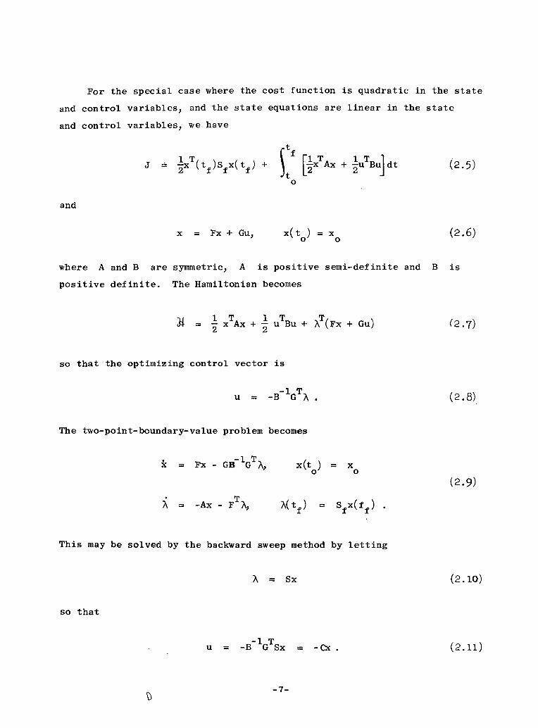
For the special case where the cost function is quadratic in the state
and control variables, and the state equations are linear in the state
and control variables, we have
xJ (tf )Sfx(tf) +
x = Fx + Gu,
0I lxTAx + 1uTBu dto
X(to) = xo
(2.5)
(2.6)
where A and B are
positive definite.
symmetric, A is positive semi-definite and B
The Hamiltonian becomes
= 1 xTAx + uTBu + T(Fx + Gu)2 2
so that the optimizing control vector is
u = -B-1GTr .
The two-point-boundary-value problem becomes
x = Fx - GB1 G T?
= -Ax - FT
x(to)= x
A(tf) = Sfx(ff)
This may be solved by the backward sweep method by letting
A = Sx
u = -B 1GTSx = -Cx.
-7-
and
is
(2.7)
(2.8)
(2.9)
so that
(2.10)
(2.11)

S is determined by a matrix Riccati equation
S = -SF - FTS - A + SGB GTS, S(tf) = Sf
The same result may be obtained by dynamic programming where we must
solve the Hamilton-Jacobi-Bellman partial differential equation
aJo= Mu ,(x v u,t)
U ? X-X;
(2.13)
J[x(tf)j tf) ] = *[x(tf)]
for the optimal return function ( the performance index expressed as a
function of the state x and time t). For the linear-quadratic problem
the optimal return function is given by
J°(xt) = 2 x S(t)x . (2.14)
B. LINEAR STOCHASTIC CONTROL
For a linear system with state x that is initially N(x , Po) (i.e.,
gaussian with mean xo and covariance matrix P ), driven by white gaussian
noise w with zero mean and intensity matrix Q(t) and described by
i = Fx + Gu + w , (2.15)
with measurements z that are corrupted by white gaussian noise v with
zero mean and intensity matrix R(t) according to
z = Hx + v , (2.16)
the conditional probability distribution of the state at time t, given
-8-
(2.12)
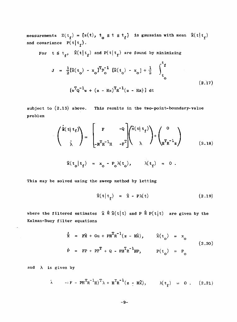
measurements Z(tf) = tz(t), to s t tf) is gaussian with mean ^(titf)
and covariance P(tltf).
For t _ tf, x(tltf) and P(tltf) are found by minimizing
to
(2.17)
[wTQ-lw + (z - Hx)TR-(z - Hx)] dt
subject to (2.15) above.
problem
This results in the two-point-boundary-value
(x(t /tf)\ H F
. IHTR-1H
0 R
HR - z (.8
x(toltf) = x - Po (to), A(tf) = o .
This may be solved using the sweep method by letting
x(tltf) = ^ - (t)
where the filtered
Kalman-Bucy filter
estimates ^x ^x(tlt) and P - P(tlt)
equations
are given by the
A Tx = Fx + Gu + PHTR-l(z - Hx),
P = FP + PF + Q - PH R-HP,
(t) = x
p(t ) =
and A is given by
A -F - PHTR-1H)T + HTR l(- H), h(tf) - O .
-9-
(2.19)
(2.20)
(2.21)
(2.18)

x(tltf) is then given by (2.19), and P(tltf) is given by
P(tltf) = P + PAP
where A is determined by
A = -(F - PHTR-1H)TA - (F - PHTR-1H) + HTR-H, n tf) = 0 . (2.23)
For the prediction case where t > tl, x(tltl) and P(ttl1) are deter-
mined by
x(tltl) = Fx(tltl) + Gu
x(tlIt1 ) = X(ti) ;
(2.24)
P(tltl ) = FP(tltl) + P(tltl)F + Q
P(tlltl
) = P(tl)
If we let our
cost function
performance index be the ensemble average of a quadratic
tf
J = EC = E{~xT(tf)Sfx(tf) + I [ixTAx+ iuTBuldt}
then the separation theorem tells us that the optimal control is the
Kalman-Bucy filter followed by the optimal deterministic feedback controller.
oFor the optimal control u to be realizable, it must be a functional
of Z(t) [the measurements up to time t, z(T), to 0 T S t], and our initial
information about the system. However, this would appear to imply that
(2.15) is no longer Markovian and Dynamic Programming techniques (as well
as calculus of variations techniques) are no longer applicable [WO-1, p. 211].
-10-
(2.22)
(2.25)
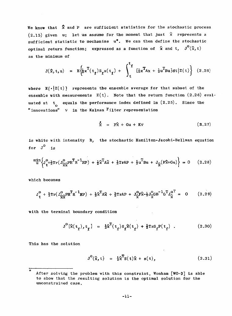
We know that x and P are sufficient statistics for the stochastic process
(2.15) given u; let us assume for the moment that just x represents a
sufficient statistic to mechanize u*. We can then define the stochastic
optimal return function; expressed as a function of x and t, J(fit)
as the minimum of
t
J(%t,u) = E{u xT(tf)Sfx(tf) + [x"Ax + 1uTBu]dt|Z(t)} (2.26)
where E{.IZ(t)) represents the ensemble average for that subset of the
ensemble with measurements Z(t). Note that the return function (2.26) eval-
uated at t equals the performance index defined in (2.25). Since the
"innovations" V in the Kalman Filter representation
x = FR + Gu + KV (2.27)
is white with intensity R, the stochastic Hamilton-Jacobi-Bellman equation
for Jo is
u {Jt+iTr(J^)PH R HP) + lx Ax + ITrAP + u Bu + J^(Fx+Gu) = 0 (2.28)
which becomes
O o T -1 1 T,- T oTJ + ITr(J^PH R HP) + 1x Ax + ½TrAP + J^Fx-2J^GB G J^ = 0 (2.29)t 2 xx X x x
with the terminal boundary condition
J x (tf),tf] = (tf)sf(tf) + ^TrSfP(tf) . (2.30)
This has the solution
J(t)= 2x S(t)x + s(t), (2.31)
After solving the problem with this constraint, Wonham [WO-2] is ableto show that the resulting solution is the optimal solution for theunconstrained case.
-11-

where S is determined by (2.12) and s is determined by
+ TrSPHT R- HP+ +TrAP = 0
(2.32)s(tf) = ITrSfP(tf)
The optimal control is then u = -B -1G TSx = -Cx as stated by the separa-
tion theorem. The average value of the cost is then
J [X(to),t ] = ixS(t o)x + jTrSfP(tf) +
(2.33)t f
+ Tr Sf SPHTR- HP + APdt.
to
By adding the differential i dSP/dt inside the integral and adding
A[S(to)P(to) - SfP(tf)] outside the integral, we obtain
J = ½Tr(S(to)X(to) + S(t)P(t) -
(2.34)
+ tf
o
SPHTR- HP + AP + SP + SP dt.
Substituting into the above equation for S and P, we obtain
J = Tr(S(t )X(t) + SQ + CTBCP dt)
t0
(2.35)
C. NONLINEAR ESTIMATION*
For a nonlinear stochastic system and measurements of the form
This section is based on Sage and Melsa [SA-1] and Jazwinski [JA-l].
-12-
*

x = f(x,u,t) + G(x,u,t)w,
(2.36)z = h(x,u,t) + v
we may define an "extended Kalman Filter" by linearizing about the current
estimate of the state:
X = f(x,u,t) + PahT -l 7IhTI R- [z-h(X., u, t) ], X(to) = X
p = af p+paT Tf +GT ,ah -1 ah
+ GQG -- R - P,a;; aa aa^
ax ax
X=X
oh ah I=xaax ax
Two other promising methods in nonlinear filtering are, conditional
mean estimation and maximum a posteriori (conditional mode) estimation.
C.1 Conditional Mean Estimation
The conditional probability distribution of x given 2
given by Kushner's partial differential equation
P = £(p) + (h - h)TR-l(z _ h)p
where the operator £ is defined as
.tr + 1 tr+ )f GQG
Z(t), is
(2.38)
k2 .39)
-13-
where
and
(2.37)
P(to
) = P
x(to ) = xo

-1For R = O., this reduces to Kolmogorov's partial differential equation
which gives the predicted probability distribution in the absence of meas-
urements. Even though there is no known method for solving Kushner's
stochastic partial differential equation, it is useful in studying and
developing approximate solutions. Also, there is no known expression for
the conditional probability distribution of x(t) given later measure-
ments for the nonlinear system given by (2.36). From (2.38), we find that
the conditional expectation of a scalar function of x is given by
A/'. GQG/(O- O Oh) 1(.= f+ tr xx + (h - h) R (z - (2.40)
where the expectation operator ^ is defined by
(?a) - f(?)p[xlZ(t)]dx . (2.41)
From (2.40) we find that the conditional mean and covariance of x are
given by
x =f + (x- x)hR (z h) (2.42)
P f(x - ) + -(- )f + Q d X- d-
(2.43)
+ (-x -h)- xh - h)R
To evaluate (2.42) and (2.43) for the first and second moments of
p(xlZ), we would have to know all the moments. An approximate solution
for x and P may be obtained by expanding f(x,u,t), h(x,u,t), and
G(x,u,t) Q(t) GT(x,u,t) in a Taylor series. By expanding to second order
and using the fact that for nearly gaussian densities
E(XkLi7j} = PkPkij + Pik Pj + PkjPi (2.44)
we obtain the second order filter
-14-

1 2f 6hT
R-l(z - h 2h : )x -- : P + P R- - h :X= 2 a^2 c2 ,-2
* = f P + P 6fT p PhT
R- h p + GQGT +T 2GQGT-p+P-P -- -P+Yl2 ~x x 62
Fa 1ki 2
N 2 T
__ _ [hik Rj = PkjPi) l hi'J = I j~~~
and the operation : is defined by
ij
= t{. -)ij]
C.2 Maximum A Posteriori Estimation
A criterion for the maximum a posteriori estimate of the trajectory
of x is obtained for the discrete case and its corresponding continuous
criterion is found by a heuristic limiting process. The equivalent dis-
crete system is specified by
x(k + 1) = I[x(k),u(k),k] + r[x(k),u(k),k]w(k)
(2.48)
z(k) = h[x(k), u(k), k] + v(k)
where w(k) and v(k) are gaussian and
Ew(k) wT(e) = Q(k) 5 k£
(2.49)
Ev(k) vT(L) = R(k) 5k
Let X(kf) and Z(kf) denote x(ko),... x(kf) and z(kl), z(k2 ),...z(kfj
respectively. According to Bayes' rule
-15-
where
(2.45)
a 2h : P) (2.46)
6)2
(2.47)

(2.50)pIXIZ] = Pp[Z X]p[X]p[xlz] - 1ZP I
Since v(k) is gaussian
kfkl 1 expjr- (1 z(k)_h)TR-l(k)(z(k)_ h). (2.51)k-k +1 V(2i)m JRI
0
Since w(k) is a white Gauss-Markov sequence
kf
p[X] = p[x(ko)] H_k=k +1
o
p[x(k) Jx(k-l)]
where p[x(k)|x(k-l)] is gaussian with mean ~[x(k-l),
covariance
u(k-l), k-l] and
r[x(k - 1), u(k - 1), k-1]Q(k - 1) r[x(k - 1), u(k - 1), k - 1] .
The conditional probability distribution is then
p[X(kf) I Z(kf) ] = A exp{-IIx(to)_xoII2 1
0o
kf
- I E iz(k IR
-hl2ik=k +1 R-Rk)
(2.53)
+ JIx(k) - ,[x(k-1),u(k-l),k-l]lII(QrT)
where A is independent of x. Maximizing the conditional probability
distribution is equivalent to minimizing the performance index
kf
2 211 x(k0) o-II 1 + 1 Iz(k+l) - h[x(k+l),u(k+l),k+]112 k
O k=ko
(2.54)
+ Jlw(k) -1 (kQ (k)
-16-
p[z I x]
(2.52)
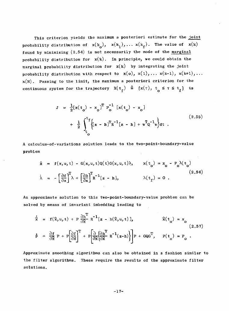
This criterion yields the maximum a posteriori estimate for the joint
probability distribution of x(ko), x(kl),... x(kf). The value of x(k)
found by minimizing (2.54) is not necessarily the mode of the marginal
probability distribution for x(k). In principle, we could obtain the
marginal probability distribution for x(k) by integrating the joint
probability distribution with respect to x(o), x(l),... x(k-l), x(k+l),...
x(N). Passing to the limit, the maximum a posteriori criterion for the
continuous system for the trajectory X(tf) A_ x('), to _ _ tf) is
J = [x(t) - To ] P [x(to ) - xo ]
t (2.55)
+ I. fi{ - h]TR-l[z - h] + wTQ-l1 dt t
o
A calculus-of-variations solution leads to the two-point-boundary-value
problem
x = f(x,u,t) - G(x,u,t)Q(t)G(x,u,t)., x(t ) = x - Po (to )
fT rTh T -ll 1(2.56)[= - f] + [ R [z - h \(tf) = O.
An approximate solution to this two-point-boundary-value problem can be
solved by means of invariant imbedding leading to
= f(^xu, t) + P 7 R 1 [z - h(x,u,t)], (to) = x
(2.57)
p7P[ -. R- (z-h)J P + GQGT, P(to) = PO
Approximate smoothing algorithms can also be obtained in a fashion similar to
the filter algorithms. These require the results of the approximate filter
solutions.
-17-

D. AN INFORMATION MATRIX APPROACH
The approximate filters of the previous section were derived on the
assumption that the covariance/is "small" compared to the nonlinearities
in f, G, and h. For example, in the scalar case, a "smallness" criterion
could be obtained by expanding f(x) to second order about x:
I 2f(x) = f( ) + 2 ( ) +
x=x x=x
If the range of x-x were + 3a, then we would have to satisfy the con-
dition
4f22 xx ~ - 9f
xx
for the variance of x to be "small." Similar conditions would have to
hold for higher order terms in the Taylor series.
If the initial covariance did not meet this smallness requirement,
we could still solve (2.56) by some other technique. However, we would
still not have an estimate of the covariance of the state. Such an esti-
mate may be obtained by calculating the information matrix.
The Fisher information matrix corresponding to a probability distri-
bution p(x) is defined as follows: LVA-1, Part 1]
I - -E 2np(x) (2.58)x ax
where the expectation operator is defined as E(-) - ftf (.)p(x)dx.
If x has a gaussian distribution with mean x and covariance P,
then
P(x)=, expE-X - x) -P x x) (2.59)p(x A = (2J)nlP'
and the above definition shows us that
-18-

I = P
A general performance index of the form
J = ,f[x(tf),tf] + %o[x(to),to] +
tf
t L(x,u, t)dt
to
may be written as
J = J(-) + J(+)
where J(-) and J(+ ) are defined by
= 0o[x(to),t0 ] +
= *f[x(tf),tf] +
Itf
t
L(x,u, t)dt
(2.63)L(x,u,t)dt.
The adjoint variables are equal to [BR-1]
XT(t) = (t) and AT(t) = - x(t) (2.641
Let us make the assumption that the conditional probability distrib-
ution of x(t) given measurements Z(tf), is given by*
p(x) = Ae -J (X) (2.65,'
where A is independent of x.
This is not strictly trueterion for the trajectoryprobability distribution,
sinceX(t)
x(t).
J is the maximum a posteriori cri-and not a criterion for the marginal
-19-
C
(2.61)
(2.62)
J(-)(t)
J(+)(t)
*
(2.60)

The information matrix for x(t), given measurements Z(tf), may then
be expressed as a function of the performance index (2.55) by
I (tltf) = E
x=x
aJ
x(tf,)
(2.66)
(2.67)aJ(-)(tf ) aXJ(t(t ) ax(tf)
we have
I (tf) s I (tftt ) = -E m .
The sensitivity matrix 3a(t)
E ax(t)wo-point-boundary-value problem
is specified by the linear matrix two-point-boundary-value problem
X = ([ ] - M)X - GQGTA,
A = (-N - v R E )X - [zfA
X(tf) = I
A(to) = -p X(to)
(2.68)
(2.69)
A 6x(t)ax(tf)~XTt and A(t) A E F(t)
= E 7A(tt)
T T Tthe ith row of M = A (m i/x), where mi = ith row of GQG , and the
T ' ' T ~ - Tith row of N = (n/~x), where n. = ith row of [(6f/x)] . Once
the TPBVP of (2.56) is solved, the coefficients in (2.69) may be evaluated.
D.1 Linear System
As an example, consider the linear system and measurements specified
by
-20-
Since
where
X(t) (2.70)

x = Fx(2.71)
Z = Hx + v
with the performance index
J [X(to)-xo]TP-1 [x(to)-x] + I (z-Hx)TR-l(z )dt . 2.72)
0
The vector TPBVP for x and A is
= Fx \(to) -P-1 [x(to) x ]
o 0 0 0
= -FTA + H R-(z-Hx), (t) = , (2.73)f
and the matrix TPBVP is then
X = FX, X(tf) = I
(2.74)
A = -FTA - HTR -HX, A(t ) = -P X(t)
and the information matrix is
Ix(tf) = -A(tf) . (2.75)
Now let us verify that this answer agrees with what the Kalman filter
would give: Let
fxx xA
be the transition matrix for
F 0_HTR
-
1H -FT
so that
X(t ) = oxx(toltf)X(t2f) (2.76a)
-21-

A(tf) = 4½x(tfto ) X(t o ) + Ak(tfto) A(to ) .
Making the substitutions
= I and A(to) = -PO1X(to )
A(tf) = [*xO(tf to ) - ( tf, to)P 1] xx(to, tf)
Differentiating
= [-HTR 'H xx(tfI to)- FT (tft ) + F o(tfo t )Po-1
+ [IA(tf,t ) - (tf, t o)Pol] xx(to, tf)(-)F
and simplifying
^ A(tf) = -HTR-1H - FT A(tf) - A(tf)F
we find that-1I satisfies the equation for P in the
xKalman filter:
I = -I F - FTIx x x
+ HTR-1 H I (to) = p-1
x o o(2.80)
For this simple example, a direct* derivation of J is easier;
readily leading to
Ix(t ) = 2 Jx~f x2 (tf)
t f
toT P- (t(t)H R0HX(t)dt0
and only the first equation in (2.74) is needed. Differentiating, we have
By "direct" we mean that the performance index is differentiated directlywithout employing the adjoint variables.
-22-
(2.76b)
X(tf)
we have
(2.77)
^ A(tf)
(2.7.8)
X xx(tItf)
(2.79)
(2.81)

to); I (t x) ='to)P X ( xT(t )H TR HX(tf)
f XTHTR 1HX + XTHTR HXdt. (2.82)
0
If we make the substitutions
X(t>) a (e ) ext F = -X(t)F
and (2.83)
X(tf) = I
we obtain (2.80).
E. NONLINEAR STOCHASTIC CONTROL
If we assume that R and P given by (2.37), (2.45), or (2.57) repre-
sent a set of sufficient statistics for p(x,tJZ), and z - h(x,u,t) is
approximately white with intensity R, then we can form the stochastic
Hamilton-Jacobi-Bellman equation. This makes the problem nearly impossi-
ble to solve. If we cannot make assumptions such as this there is no
known "exact" method of solving the nonlinear stochastic control problem.
The performance index for the nonlinear problem may also include
weights upon the moments of the cost as well as just the mean of the cost:
J = %lEC + a2E(C - C) + .. anE(C -_ )n + ... (2.84)
In practice, this performance index could be expanded to second order as
is done in the second-order filter.
-23-

Chapter III
STRUCTURE DETERMINATION
A. INTRODUCTION
Recall from Chapter I that the first task of mathematical modelling
is the determination of the system structure. In many applications, the
order and structure of the differential equations may be derived from
physical principles. Such is the case in deriving the equations of motion
of an airplane.
In more complex systems such as biological or economic processes, the
underlying processes are not well known. In such cases, an approximate
model of the system may be obtained by assuming a given order or other
structural information about the system and fitting data to it.
Let us assume that the structural information about the system may
be specified by a set of model numbers. An example of a model number,
other than the order of the system n, the number of inputs p, and
the number of outputs m, would be the order r of the minimal annihi-
lation polynomial.* A possible method of determining the structure of a
system is the following:
(1) Assume a given value for the model numbers (for example,assume a first order system).
(2) Perform the other two tasks of mathematical modelling underthis assumption, namely (a) choosing an input and measuringthe corresponding output, and (b) identifying the parametersof the assumed structure from input-output records.
A polynomial is an annihilation polynomial if it equals O when theF matrix is substituted for the independent variable. The Hamilton-Cayley theorem tells us that the nth order polynomial of the character-istic equation is an annihilation polynomial. However, there may beother polynomials of lower order that are also annihilation polynomials.
-24-

;3) Increase the values of the model numbers (for example, increasethe order by one) until a structure criterion is met. Twopossible structure criteria are: (a) the residuals (differ-ence between the measured output and model output) are "close"to being white. Such a criterion has been used by Mehra [ME-1];(b) There is no significant reduction in the identificationcriterion. A significance test for the reduction is given inAstrom and Eykhoff [AS-1]. The latter criterion appears tobe the more decisive [SP-1] but requires an identification atone higher value of the model numbers than the former criterion.
The next section discusses useful results from realization theory
that may be applied to constructing canonical forms. It also discusses
the construction of canonical forms with four model numbers (m, n,
p, and r) and compares the canonical forms of Denery and Spain.
B. REALIZATION THEORY*
Realization theory for deterministic systems is concerned with
specifying the internal description of a system (i.e., specifying its
differential equations) from a known external description of a system (as
expressed by its impulse response matrix or transfer function matrix). For
the deterministic system
x = Fx + Gu
(3.1)y = Hx
with zero initial conditions, the output is given by
t
y(t) = | H*(t,¶)G u(r)d¶ (3.4)
o
or in the frequency domain, by
y(s) = H(sI - E) 1Gu(s) . (3. )
This section based on Kalman [KAIrl].
-25-

As far as any input-output relationships are concerned (with zero
initial conditions), the descriptions in (3.4) and (3.5) are equiva-
lent to the description in (3.3). However, the specification of
'(F, G, H) from either (3.4) or (3.5) is not unique. Before proceeding
with the main results of realization theory for linear time invariant
systems, two definitions and one theorem are in order.
1. Definition 1:
(F, G, H) is strictly algebraically equivalent to (F, G, H) if
and only if there exists a non-singular constant matrix T, such that
_- -1F = TFT
G = TG (3.6)
H = HT
2. Definition 2:
(F, G, H) is a minimal realization if there is no other realization
(F, G, H) with an F of order smaller than the order of F.
3. Canonical Structure Theorem
The state vector may be transformed into four mutually exclusive
parts (see Fig. 3.1):
Part A: controllable but unobservable;
Part B: controllable and observable;
Part C: uncontrollable and unobservable;
Part D: uncontrollable and observable;
so that F, G, and H take the canonical forms
-26-

I i
! I
I I
II
P~~~~~~~~~~~~~~~~~~~~~~~~~~~~~~~~
FIG. 3.1. DIAGRAM OF CANONICAL STRUCTURE THEOREM
-27-
lI
FAB FAC FAD
O F BB
o o
BDO F
F F
0 0 FDD
O HD
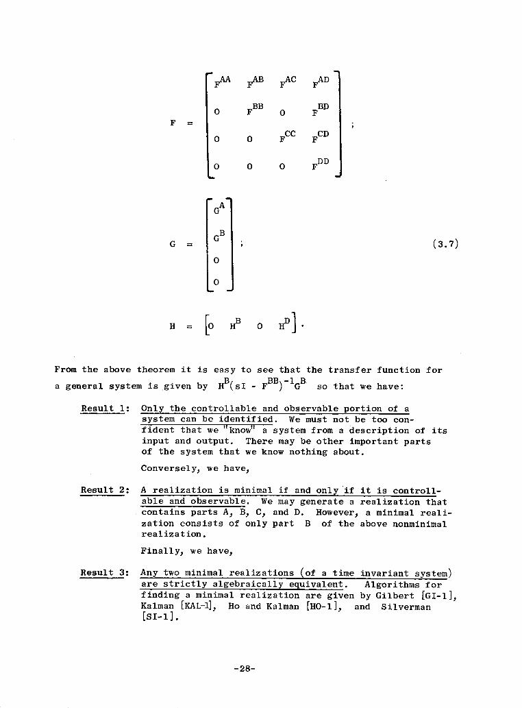
From the above theorem it
a general system is given
Result 1:
Result 2:
Result 3:
is easy to see that the transfer function for
by H (sI - F ) G so that we have:
Only the controllable and observable portion of asystem can be identified. We must not be too con-fident that we "know" a system from a description of itsinput and output. There may be other important partsof the system that we know nothing about.
Conversely, we have,
A realization is minimal if and only if it is controll-able and observable. We may generate a realization thatcontains parts A, B, C, and D. However, a minimal reali-zation consists of only part B of the above nonminimalrealization.
Finally, we have,
-28-
FAA
LO
G =
GA
GB
0
0o
Lo
(3.7)
H = [O HB
Any two minimal realizations (of a time invariant system)are strictly algebraically equivalent. Algorithms forfinding a minimal realization are given by Gilbert [GI-1],Kalman [KAL-1], Ho and Kalman [HO-1], and Silverman[sI-1].
J

There are at least three main criticisms of the realization theory
approach to mathematical modelling: (1) The transfer function (or impulse
response) matrix has to be determined before it can be applied. Why
not identify F, G, and H directly from measurements of the inputs and
outputs without first calculating the transfer function matrix? (2) It
is assumed that the transfer function (or impulse response) matrix is given
exactly; whereas with these external descriptions, the parameters in F,
G, and H may be very sensitive to small errors in the transfer function (or
impulse response) matrix. (3) One may be led to believe that an impulse
or sine input is the "proper" input to use.
C. MINIMAL PARAMETER SET
In parameter identification the number of independent parameters q,
needed to describe a system, is of great interest. If a realization is
of minimal order, any desired canonical form can be used to enumerate
the number of independent parameters. The information matrix provides a
means of verifying the identifiability of a set of parameters. The
independence of a set of parameters in the information matrix is equivalent
to the identifiability of the parameters. If the information matrix for
a set of parameters is singular for any input, then we do not have a
canonical form.
By knowing the order n, number of inputs p, number of outputs
m, and part of the structure of a system, Denery [DE-2] constructs a
canonical form involving n(m + p) parameters. The structural information
needed consists of the first n linearly independent rows of the observa-
bility matrix. If we do not know the first n linearly independent rows,
then we must examine each possibility for a given value of n.
For systems with an annihilation polynomial of degree r (but of un-
known order n ) r), Spain [SP-1] constructs a canonical form involving
r(mp + 1) parameters. If F has an annihilating polynomial of degree
less than n, then F is similar to a quasidiagonal matrix that has two
or more Jordan blocks with the same eigenvalue. It would then seem to be
a special case for a physical system to have r < n. Thus, Spain's number
of parameters is much larger (for multi-input multi-output systems) than
Denery's, except for special cases. However, Spain does not assume any
structural information and would not have to investigate a large number of
cases for each value of r.
-29-

Any square matrix with multiple eigenvalues is similar to a quasi-
diagonal matrix where each diagonal matrix is a Jordan matrix. The
possibility of multiple eigenvalues suggests that this form gives us a
form with the minimum number of parameters. It is instructive to cal-
culate the number of parameters needed to describe a quasidiagonal canonical
form for the model numbers (m, n, p, r). The results are shown in
Table 3;1 for n = 1, 2, 3. For n 2 4, the number of cases increases greatly;
for example, for n = 4, there are 14 different cases and for n = 5
there are 29 different cases. For each case, the number of parameters
is less than or equal to that given by Denery or Spain. (Since each of
these cases assumes more about the system.) A method of calculating the
results shown in Table 3.1 is illustrated in the following example: Find
the number of parameters needed to describe a second order system with
two inputs and two outputs. There are three different cases:
Case 1: Distinct eigenvalues. See Fig. 3.2a, (r = 2). As far as
input-output relationships are concerned, we could make the following
replacements:
gll gll hll h 11 I
g12 - g12 h22 h21 /hl
-21 g21 h 1 1 h1 2 h12/h22
g22 g22 h22 2222 22 1.
For this case there are eight parameters: X1, X2, gll, g1 2' g21'
g2 2, h 12 , h2 1 . The information matrix for these eight parameters isnonsingular.
Case 2: Jordan form. See Fig. 3.2b, (r = 2). In this case we make
the following replacements:
-30-

Table 3.1
The minimal number of parameters, q, ofform for the model numbers (m, n, p, r).shown for n = 1, 2, 3. For each case, qversus m and p.
a canonicalCases areis shown
Order and Case F Matrix q vs. m and pI I I I A~~~~~~~~~~
Lx]
XI1 X
0 X2
0o
1
X
0 X
m = number of outputsn = order of systemp = number of inputsr = order of minmal annihi-
lation polynomial
1 2 3 4 5
\m1I 2 3 4
1 4 6 810
2 6 8 10 12
3 8 10 12 14
4 10 12 14 16
m 1 2 3 4
1 4 6 8 10
2 6 8 10 12
3 8 10 12 14
4 10 12 14 16
m 1 2 3 4
32 5 7 9
3n 79 -11J
4 9 11 13Contd.
Not Observable
Not Controllable \\-\
-31-
pNn= 1Case 1r = 1
n = 2Case 1r = 2
n = 2Case 2r = 2
n = 2Case 3r = 1
1 2 3 4

Table 3.1 (Contd)
Order and Case F Matrix q vs. m and p
n= 3Case 1r = 3
n = 1, Case 1 E
In = 2, Case 1 J
n=3Case 2r=3
[ n = 1, Case 1
In = 2, Case 2 i
n= 3Case 3r = 3
n= 3Case 4r = 2
n = 1, Case 1 I
[n = 2, Case 3 .
O 0
X2 0
0 3
0 0
X2 1
0 X
1 0
X 1
o X
0 0
X20
0 X2 J
2 3 4 _
1 6 9 12 15
2 9 12 15 18
3 12 15 18 21
4 15 18 21 24
1 2 3 4
1 6 9 12 15
2 9 12 15 18
3 12 15 18 21
4 15 18 21 24
m 12 3 4
1 6 9 12 15
2 9 12 15 18
3 12 15 18 21
4 15 18 21 24
m 1 234
2 9 12 15
3 12 15 18
4 151821
0
[1
0
0
X1
0O
0
X
l O
Contd.
-32-
I1

Table 3.1 (Contd)
-33-
Order and Case F Matrix q vs. m and p
4 R 14 17 20
n= 3 _ 0 m1 2 3 4Case 6 1r=1 12 0
0 3 1013
4 13 16
O O X~~~~~~~~ 4 ' 1

Fig. 3.2a
Schematic diagrams for an example in deter-mining the minimum number of parameters of acanonical form. The example was a secondorder system with two inputs and two outputs.
-34-
z1
z 2
z2
z2
FIG. 3.2.

1g1 - gll hll hll 1 , 1
g12 g12 h h21 21 h 11/h
g21 g21 h11 12 ll12/h 11
-22 g2 2 h1g h2 2 h22/h 11
In this case we cannot normalize with respect to h22 due to the extra
coupling; however, both eigenvalues are the same so that eight parameters
are still all that is necessary; namely, X, gll, g1 2, g2 1, h 1
2 ,
h 21 , h 2
2 '
Case 3: Two (1 X 1) Jordan blocks have the same eigenvalue. See
Fig. 3.2c, (r = 1). From the results of Case 1, we know that seven
parameters are sufficiently general; but perhaps they are not all iden-
tifiable. From Fig. 3.2c, we see that as far as the paths from ul to z
are concerned, we cannot tell from measurements of the input and output
whether we took path gl l - 1 or g1 2 - h1 2. We may eliminate one
path by setting hl2 = 0 (if it is not needed by some other connection).
In going from u2
to z2' we reach a similar conclusion about h
2 1. In
going from u1 to z2, we have to keep either g12 f 0 or h21 f 0; let
us choose g12 A 0 and h2 1 = O. From u2 to Zl we reach a similar con-
clusion about setting h1 2 = O. We thus have the possible form shown in
Fig. 3.2d, with five parameters: X, gll1 g1 2, g2 1, g
2 2. The informa-
tion matrix for seven parameters can be shown to be singular for any
input. This is a consequence of the linear dependence of the sensitivity
equations when X1 = X2. For the set of five parameters, the information
matrix is nonsingular.
Although the results in this example were derived assuming that the
eigenvalues were real, we would get the same number of parameters since
for each complex eigenvalue, its conjugate is also an eigenvalue. Note
-35-

Up s -x 1 1
s -X
Fig. 3.2c
zs - X
Figs.- X 1~--- z 2
Fig. 3.2d
Schematic diagrams for an example in deter-mining the minimum number of parameters of acanonical form. The example was a secondorder system with two inputs and two outputs.
-36-
U
u2
U1.
U 2
FIG. 3.2.(Cont)

that for all cases for which no Jordan blocks have the same eigenvalue
(i.e., for which r = n), the number of parameters is the same as that
given by Denery's canonical form, q = n(m + p).
Future research would be useful in determining the best model numbers
for multi-input multi-output systems. Considerations should answer the
following two questions: (1) What is the minimal number of parameters,
q, needed to designate an arbitrary member of the class defined by the
model numbers? (2) As the order of the system increases, how many differ-
ent cases, c, must be examined? In general, the more model numbers we
have, the smaller q is but the larger c is. Some optimum trade-off
should be possible.
-37-

Chapter IV
IDENTIFICATION CRITERIA
A. INTRODUCTION
Let the vector, a, represent the unknown parameters in F, G, H,
Q, and R (and the initial conditions) , and Z(t) the set of measure-
ments up to time t. The identification criteria developed in this
Chapter are based on finding the value of a at the maximum of the
a posteriori probability distribution Plz :
a = arg max P aZ .
This is a mathematically simpler approach than the conditional mean
approach summarized in Chapt. II.C. Since a is a vector of constant
parameters, we do not have the problem noted in Chapt. II.C that there
may be a difference between a maximum a posteriori criterion for the
joint probability distribution and the marginal probability distribution.
Since Bayes formula tells us that
PZ = Pa
·aIZ (4.1)pz
the maximum a posteriori equation is
- nnpZa
npa
+ = o . (4.2)
The classical maximum likelihood criterion is to choose that a for which
Pzla is a maximum. The maximum likelihood equation is then
-38-
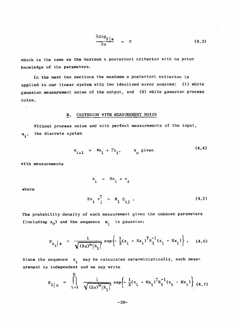
2nPZ a= 0 (4.3)
a
which is the same as the maximum a posteriori criterion with no prior
knowledge of the parameters.
In the next two sections the maximum a posteriori criterion is
applied to our linear system with two idealized error sources: (1) white
gaussian measurement noise of the output, and (2) white gaussian process
noise.
B. CRITERION WITH MEASUREMENT NOISE
Without process noise and with perfect measurements of the input,
ui, the discrete system
Xi+ 1 = x1 + rui, x given (4'4)
with measurements
z. = Hx + v
where
TEv vj = R 5i . (4.5)
The probability density of each measurement given the unknown parameters
(including xo) and the sequence u. is gaussian:
zila 1 ex -(Z Hxi) R1 (Z Hxi)} * (4.6)
Since the sequence xi may be calculated deterministically, each meas-
urement is independent and we may write
N
il ()mR exp 1 - Hx ( - Hx~ZIa 1 p=- - zn Hxi)TR l~z.2 i (4.7)i=l 2iRj
-39-
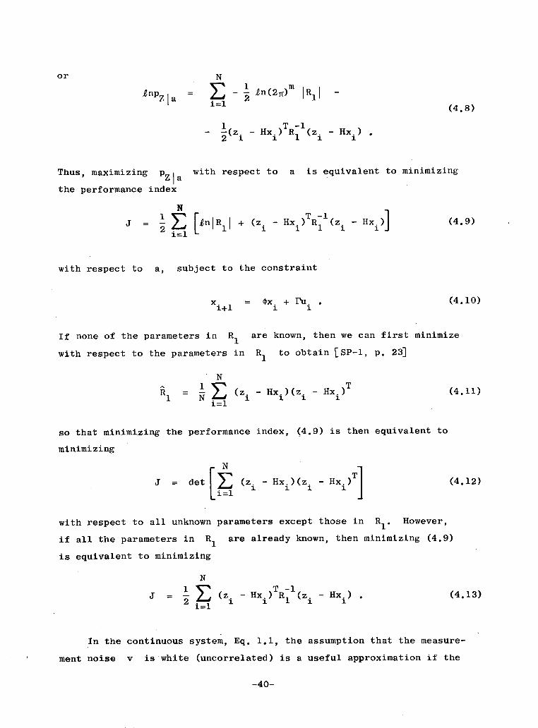
or N
npZa = E n(2)m IR11
(4.8)
1 T-l2(Zi - Hxi) R1 (Z
i- Hxi) .
Thus, maximizing Pzl with respect to a is equivalent to minimizing
the performance index
N
2 i1l [n R1, + (z. Hxi)T R1 (z - Hx.) (4.9)
with respect to a, subject to the constraint
xi+l = (x. + Pui . (4.10)
If none of the parameters in R1
are known, then we can first minimize
with respect to the parameters in R1
to obtain [SP-1, p. 23]
N
1= (N i - Hxi)(zi Hx)T (4.11)1
so that minimizing the performance index, (4.9) is then equivalent to
minimizing
J = det (zi - Hxi)(zi - Hxi)T (4,12)
with respect to all unknown parameters except those in R1 . However,
if all the parameters in R1
are already known, then minimizing (4.9)
is equivalent to minimizing
N
J - (z. - Hxi) R1 (zi
Hx) . (4.13)
In the continuous system, Eq. 1.1, the assumption that the measure-
ment noise v is white (uncorrelated) is a useful approximation if the
-40-

correlation times of the measurement noise are short with respect to the
dynamics of the system being measured. However, in trying to estimate
the intensity matrix R, the assumption about independent measurement
errors is invalid as the measurement interval tends to zero. This is
reflected in the fact that the limit of (4.9) does not exist. However,
we can estimate R by thinking of v as a correlated process with a
very short (but finite) correlation time. In this case an estimate of R
is given by
+T
R a 0 C(T) dT (4.14)-T
where the correlation matrix C(T) is given by
T-T1
C(T) T-iT v(t)vT(t + T) dt . (4.15)
The value of R is a measure of the noise characteristics of the
instrumentation, and may be obtained from measuring the instrumentation
alone, without exciting the system. For the remainder of this thesis,
R will be assumed known. With R known, we can minimize the limit of
(4.13) with R1 = R/At:
tf
J 2 (z - Hx) R ( z - Hx) dt . (4.16)
o
We are now subject to the constraint
x = Fx + Gu, x(t)= x . (4.17)
The latter performance index can also be derived by maximizing the likeli-
hood ratio [ME-2]
ZI H 1, aL -, (4.18)
PZI H0|
-41-

where HI represents the hypothesis that1
z = Hx + v
and H represents the hypothesis that0
Z = V.
The criterion developed in this section is also known as the output error
criterion [DE-2, ME-2]
C. CRITERION WITH MEASUREMENT AND PROCESS NOISE
With process noise, the discrete system (4.4) becomes
Xi+l = tXi + rUi + wi' x given . (4.19)
In calculating the correlation E(zi - zi)(z.- z.) for i . j, we
reduce the calculation to finding
,M. A - T-. E(x. - x.)(x. - x..
i E(xi Xi)(Xi 1
Refer, for the moment, to the first equation in (4.22) where M = 0o
since x is given. For the case without process noise Qi = 0, so
that M = 0 and the measurements are uncorrelated. However, with processi
noise Qi f 0, so that M.i 0, and the measurements are correlated.
Since the measurements are not independent, the probability density PZl a
cannot be equated to the product of the individual probability densities.
For this reason, a Kalman filter representation is used [ME-2]. Since
it is known that the "innovations" are white and contain all the statisti-
cal information contained in the measurements [KA-1], the probability
density PZI is given by
-42-
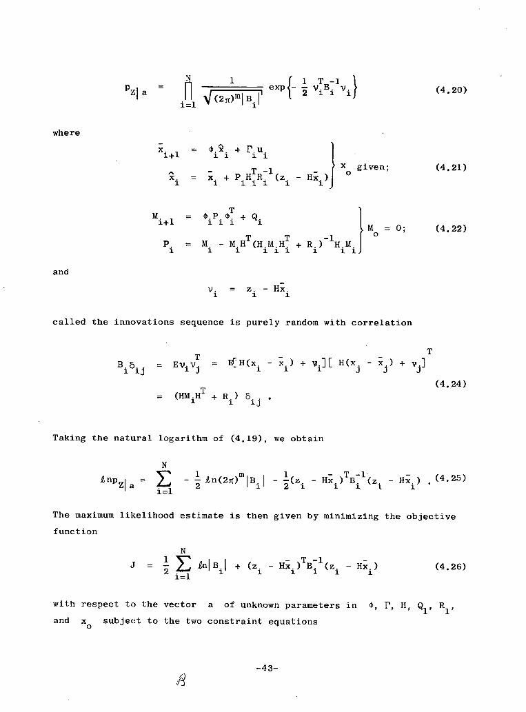
(4.20)I exp{- ViBi V i
X. = 0.x. + r.uXi+1 1 1 i
. = . + P HTR-l (z.i 1 i i 1 1
T
Mi+l 1i i + Q i
Pi = M - MHT (H.M.HT1 i 1 1 1 1
- Hx.)1
x given;
M = 0;
+ R.) -iH. M1 11
(4.21)
(4.22)
and
V. = z. - Hx.
called the innovations sequence is purely random with correlation
H(x.i - x.i) + vi] [ H(x.
T
- x.) + vJ j
= (HMiH + Ri) ij.1 13
Taking the natural logarithm of (4.19), we obtain
N
tnPZJ a = Ei=l
m ~ 1 -i) -12 n(2O)mIBi 2(zi -Hxi) B. (z. - Hi) .
The maximum likelihood estimate is then given by minimizing the objective
function
N
2 =nE nBi + (Z.2=l
-Hxi) Bi (zi - Hx.)1 1~~
with respect to the vector a of unknown parameters in 4, P, H, Q1 , R1,
and x subject to the two constraint equationso
-43-
PZJ a
where
BiBij
T= EV i Vj
(4.24)
(4.25)
(4.26)
N
= ni=l

Xi+l xi + U + [Mi - MiHT (HM HMiH+R1) i](HTR(z-H)
x = x ; (4.27)
Mi+l = L[Mi - M1HT(HM i HT+ R 1) - HMi]J + Q M =
If we can make the assumption'that Mi is a constant, then consider-
able simplification results. This will eliminate the second set of con-
straint equations in (4.27). This assumption will be a good one if the
test is conducted over a long time interval so that Mi is nearly con-
stant for most of the test. However, if this assumption is not valid, then
we must solve the problem as formulated above.
In the "steady state Kalman filter representation" [ME-2], we can
identify B and K instead of R1
and Q1 where B and K are given by
B = HMH + R1, and K = MHTB and M is the solution to
M = M - MH (HMH + y i HM]h + Q1
Note that the above equations cannot be solved uniquely for Q1. Our
problem now becomes: minimize the performance index
N
J = 2iE [lnIBI + (Z Hx)T B-l (z - Hx.) (4.28)
with respect to the parameters in 4, P, H, B, K, and xo, subject to
the constraint
xi+l= x. + Pu. + WK(z. - Hx.) . (4.29)1 1 1
For the continuous case we can proceed in a similar manner. If we
assume that R is known, then the identification criterion for the
steady state Kalman-Bucy filter representation is to minimize
-44-

tf1
J = 1 (z - Hx)TR- (z - Hx)dt2 t
(4.30)
with respect to the unknown parameters in F, G, H, K, and x subject to
the constraint
x = Fx + Gu + K(z - Hx), x(t ) = x0 o
As in the discrete case, if the assumptions regarding the steady state
are not valid, then we must include the covariance equation as another con-
straint.
This criterion could also be derived by employing the criterion for
the maximum likelihood estimate of a and the trajectory x(t), t o t < tf.
In this case we want to minimize
= [x(t)-xo] P [x (t ) - x ]2 = 2 [ X0to o o
1 tf T -1+ Lw Q w +
-to(z - Hx)TR-1(z -
with respect to a and w(t), t ' t < tf; subject to0 _t;sbett
x = Fx + Gu + w .
By performing the minimization first with r
Kalman-Bucy filter equations
= T -lx = Fx + Gu + H R (z - Hx),
P = FP + PFT + Q -TR-1H HP,
espect to w(t), we obtain the
(t ) = xo o
(4.34)
P(t ) = Po o
and the equation for the adjoint variable
-45-
(4.31)
(4.32)
Hx) dt
(4.33)

X = (- pHTR- PH H) + HTR-(z - Hx), X(tf) 0 . (4.35)
TIf we substitute w = -QGTX and x = x - P into (4.32), and add the
differential
dt
inside the integral and
T TX (t ) P(t ) X(t ) - T (t ) P(t ) X(t )
outside the integral, we obtain (4.30). Our identification criterion then
is to minimize (4.30) with respect to a, subject to (4.34). The
adjoint equation (4.35) is not considered a constraint for the minimiza-
tion with respect to a since X is not in (4.30) or (4.34). Once the
maximum a posteriori estimate of a has been found, the smoothed
estimate of the trajectory using a = a is the maximum a posteriori
estimate of the trajectory.
If we assume perfect measurements of the state and derivatives of
the state are taken, then the criterion of (4.32) and (4.33) may be re-
duced to minimizing
tf
J = 1j (k - Fx - Gu)TQ- (x - Fx -Gu)dt
t
with respect to the unknowns in F and G. Since the unknown parameters
in F and G are quadratic in (4.36), estimates may be obtained in one
step. This criterion is a special case of the criterion discussed in
this section and is known as the equation-error criterion [DE-2 and ME-2].
D. CRITERION WITH PRIOR INFORMATION
To incorporate prior information, let us use the maximum a posteriori
equation and assume a prior probability distribution that is gaussian with
mean a and covariance A:
-46-

P (2 )A1 exl{ 2(a-l) Al(a)} (4.37)Pa2
or
nanp n - --l(a-a)TA- 1(a-a) . (4.38)a22
The performance indices are then modified to include the additional term
1 -T -l (a - a) A- (a - a)
and the constraint equations remain the same.
-47-

Chapter V
IDENTIFICATION ALGORITHMS
A. QUASILINEARIZATION*
Denery [DE-1] combines two different linearization techniques to
minimize the.output error performance index
1 tf (z - A)TR(z - ^)dt
0
(5.1)
where the system is modelled by
x = Fx + Gu, x(t ) = xo o
(5.2)
and z is a given set of measurements. J is minimized with respect to
the unknown parameters in F. G, H, and x , subject to the constraints
in (5.2). His first linearization technique may be considered an exten-
sion of quasilinearization. Instead of modelling the system as given by
(5.2), ^z is instead modelled by
x = Fx + Gu + D(z-Hx) =. F x + Gu + Dz,n
z = iH+L(z-Hx) = = x+Lz
(t ) = x
(5.3)
where
Denery's combined algorithm [DE-1].
-48-
*

F = F - DHN
(5.4)
HN H - LH .
This set of equations is useful only if the system (2) is in a Denery
canonical form. Now, let
G = G - GN
N (5.5)
8Xo o XNo
and define zN by
XN = FNXN + GNUl XN(to) = XNo(5.6)
ZN = HNX N
If we guess FN, GN, HN, and XNo, the unknown parameters are now in D,
5G, L, and bx instead of F, G, H, and x . By augmenting the system0 I
equations with the terms D(z-H^) and L(z-Hx), Denery was able to make
the unknown parameters coefficients of known functions so that we may write
z = zN + (5.7)
where a is a (q X 1) vector representing the unknown parameters in
6G, 5x , D, and L. The ith column of the matrix (6z/3a) is given by the
sensitivity equations
a X aD 6ascGu a0 t \(E = FN(v) + EZ+(v)u(F + , (to
N1 ) 1 -(t) 1.
(5.8)
(v7) N(i-) + i -bz H ~
11 1
-49-
Notice that in this formulation, the sensitivity equations are driven by
the actual measurements z. Taking the derivative of the performance
index with respect to the unknown parameters,
t f
Z-a to
( - ) TR- (--) dt = 0
and substituting (5.7) into the result yields
Stf (z)T -l(^) Itto
tf
( (a] )Tl (z ZN)dt0
so that an estimate of a is given by
A [s t ft1fdt] [s (h) r T]a = R d )Rl d
7a ) 7a)t a z-0
An estimate of the unknowns
ploying (5.4) and (5.5):
in F, G, H, and x 0is then given by em-
G = GN + G
XNo 0
H = (I- HN
F = FN
+ DH
(5.11)
These estimates may then be used as nominal values in another iteration.
This approach was found to be convergent even for large inaccuracies
in the initial guesses of the unknown parameters. However, the estimates
given by this method are biased even if the noise is unbiased (i.e., has
zero mean value).
-50-
(5.10)

After three or four iterations of using this extended quasilineariza-
tion technique, Denery suggests switching to the normal quasilineariza-
tion technique. In the method of quasilinearization, z is represented
by (5.2) but approximated by small deviations from the nominal by
= HNXN
+ (H- HN)x + HN6x = HNxA + (H-HN)x (5.12)
where xA - xN + 8x xN is given by (5.6), and 8x is determined fromwe xA = N + * N
8x = FN8x + (F-FN)x + 8Gu, 8x(t) = xo0
so that xA is determined from
xA = FNXA + (F - FN)XN + (GN+ 8G)u, xA(to) = XNo + 6x
(5.14)
For quasilinearization, we assume that F - FN
and H - HN are small so
that for a system in a Denery canonical form, we may write
F - FN
= DH = D(HN + LH) - DHN
(5.15)
H - HN = LH = L(HN + LH) - LHN
where D and L are small. Now substituting these into (5.14), we have
XA = FNXA + DzN + (GN+SG)u,
= Hx A + LzN
xA(tO) = XN. + 8X
(5.16)
This equation is identical to (5.3) except that zN has replaced z. The
solution is the same as the extended method except that zN
drives the
sensitivity equations (5.8) instead of z.
The estimates obtained using this method are unbiased but the method
often does not converge if the initial guesses of the unknown parameters
-51-
(5.13)

are far from their true values. Thus, it can be used after the first
method to obtain a combined algorithm insensitive to inaccuracies in the
initial values of the unknown parameters and yielding an unbiased estimate.
In summary, to find an estimate for F, G, H, and x with initialo
guesses given by FN, GN, HN, and xNo:
1. Calculate a nominal trajectory
XN = FNXN + GNU' XN(to) = XNoper(5.6)
ZN = HNX N·
2. Calculate the sensitivity functions given by z or zN
Z(n) +(Ti)u,I (6v)(to) = 6-Ta-. )aper(5.8)
= HN( + ) + (n) i 1
3. Calculate an estimate of the unknown parameters in 5G,; Xo, D,
and L:
Aa = Ftf T= ) R- 1
o
4. Calculate estimates of
val ues in the next iteration
per(5.10)
the parameters that can be used as nominal
G = G + N
X0 XNo
H = (I - L)- HN
F = FN
+ DHN
per(5.11)
-52-
/ 16 .ax) aD.1 1
i = 1J 2 ... q .
( ) R (Z-ZN)dt .

The amount of computation per iteration involves n + n. q + ½q(q+l) + q
integrations over the length of the test.
Example: Identify the constant, a, in the first order system:
x = -ax + au, x(O) = 0
z = x + v
where Ev(t)v(-) = r8(t - T). Note that this example is slightly different
from our development, since the same parameter is in F and G. Augmenting
the state equation with D(z-2), we have
x = -a^ + au + D(z-x) = -(a+D)x + au + Dz
Now,G = G- G
N= a- a
N= -D .
Let
6G = a so that M= 1 and
= 1 and - -1 .
The nominal and sensitivity equations are
XN = -aNXN + aNu,
(!~)(anx\= -a N() + -
z
xN(o) = 0
E (o) =O .
An estimate of a is given by
a = [Stf ) d t
An updated estimate of a (which can
next iteration) is given by
Va/[ kz - xN)dt
be used as a nominal value for the
-53-

a = aN + .
For the second set of iterations, the only change is that xN replaces
z in the sensitivity equation.
B. PROCESS NOISE
With process noise, we can represent system Eq. (5.2) by its steady
state Kalman filter
x= Fx + Gu + K(z - Hx)
(5.17)z = H.
If we proceed as before with Denery's extension, we replace (5.17) with
x = Fx + Gu + K(z - Hx) + D(z - Ix)
(5.18)z = H2 + L(z - Ix)
Obviously the sum K + D may be identified by Denery's extension but
K and D cannot be identified separately. However, we can identify
F, G, H, and x by the first quasilinearization technique, assuming that
K - 0 and proceed to the second technique.
Proceeding with the second quasilinearization method we approximate
z in (5.17) with
z = HNxN + (H-HN)xN + H8x = HNxA + (H-)xN (5.19)
where xA = xN + 8x, and xN and 8x' are given by
* = FNXN + GNu + KN(z-HN N)
N = HNX N
xN(to ) = XNo
(5.2,0)
-54-C-
and

8x = FN8x + (F-FN)X + (G-GN)u + (K-KN)(z-HNxN)
(5.21)+ KN[-(H-HN)xN - HNx], x(t
o) = xo
so that xA is given by
XA = FNXA + 8FxN + (GN+aG)u + (IKN+K)(z-HNxN)(5.22)
+ KN[(HN-8H)xN - HNXA], XA(to) = XNo + 8xo
For a Denery canonical form we can write
6F = F- FN = DH = D(HN+LH) DHN
(5.23)8H = - HN = LH = L(HN+LH) LHN
Substituting and simplifying, we have
XA = (FN INHN)XA + (GN+SG)u + DzN + KNz + 5K(z-zN)
- KNLZN xA(to) = XN+ x° (5.24)
Z HNXA + LzN
Let a represent the unknown parameters in 8G, ax o D, L, and 8K. The
sensitivity equations become
\ / ( N NH \ '/N + ZN + -u + K (z-zN) _ (5.25)
K- (Z - N)I
-55-
a, a5bxA( o
(5.25)Cont.
( - ) HN +i ZN-
Note that these sensitivity equations are driven by both z and z N. An
estimate of a is given by (5.10) where (^z/ia) is now given by (5.25)
and estimates of F, G, H, and x are given by (5.11). An estimate of
K is given by
K = KN+ SK . (5.26)
Example. Identify a and K for the first order system
= -ax + au + w, x(O) = 0
Z = x + v
and its steady state Kalman Filter representation
= -ax + au + K(z - x), x(0) = 0
For the first part of the algorithm, use the same algorithm as the previous
example, assuming that K = 0. For the second part, the nominal trajectory
is given by
XN = -aNN +
aNu + KN(Z - XN)' XN(O) = 0
where for the first iteration, KN = 0, and aN equals its identified
value from the first part of the algorithm. The approximate trajectory
is given by
-56-
XA = -(aN + KN)xA + (aN + 8K)u + DxN + K + 5K(z - xN)
XA(O) = O
A xA
Z wXA .
Let a= =G = -D
are
(A)
(ZE
and a2 = 8K. The sensitivity equations for I and a252 = K h estvt qaino 1 an 2
= -(a + )( )+ u-xN,
= -(+)( )+zxNA= -a +YN)(0 +z -x
axA7-7 (o) = 0
axA
62 (o) = O .2
Estimates ofa1 and a2 are given by
T
Io( A)\dt
T
IoT A I6xA\
0 dt\(~CX2)
/ix~k(XA\A A) d
o iA 2
-1
o S () (Z-XN)dt
O ( / (2 -XN)dt
IUpdated estimates for a and K are given by
a = aN+ +1
K = KN implementing this+ a2lgorithm is that the term
The only problem in implementing this algorithm is that the term
T~ (6xA),3-- d
-57-
a2

may be too small to allow an accurate estimate of K and the algorithm
will not converge. For xN t x, the second sensitivity equation takes
the form
x = -ax + v, x(O) = 0 ,
so that P = E(x2 ) is given by
p = -2aP + r, P(o) = O ,
orP = 2a (1 - e2at)2a
Actually, to be consistent with our steady-state Kalman filter hypothesis
of a long test, we may set
E(x ) = --2a
The covariance of K (assuming a is known perfectly) is given by
[ Tr 1K 2a j
2(aN + K
T
so that no matter what the input is we must have a sufficiently long test
to estimate K.
C. GRADIENT METHODS*
Minimize the output error performance index
t
J 1 t
f
(z - x)TR- R (z - Hx)dt0
(5.26)
First paragraph based on Sage and Melsa [SA-2].
-58-
*

subject to the constraints
x = Fx + Gu, x(t ) = x
where a' is a q' X 1 vector that denotes those unknown parameters in
F, G, and H. The lamiltonian is
= ( xT _ ) + + G) + 4 =~(z. - x) R- (z - Hx) + xT(Fx + Gu) + r · 0 ,
where
by
(5.28)
X and r are conjugate to x and a'. The adjoint equations are given
T = = (z-Hx) TR H -_ TF= xx
ri = =
xT(t ) 0 o
T -1 aH T/F G a.Ta
I I +a.-
(5.2 9)
ri(tf) = o,
i = 1, 2, ... q' .
u and z are given functions so that the Hamiltonian is not minimized with
respect to u. The gradients with respect to a' and x are given by
r(to) aJ
and x(O) = ax(t ) (5.30)
A steepest descent or conjugate gradient algorithm can now be implemented
as follows:
(1) Guess an initial value for a' and x ;
(2) Calculate x by integrating (per Eq. 5.27),
' = Fx + Gu, x(to) = XO
(3) Calculate the adjoint equations (per Eq. 5.29)
-59-
(5.27)a' = 0
= H R-(z - Hx) - F X,
T 6HT R-IzHx) T _ [ T TTG= x -~R- (z-Hx) - Ex aFT +U GT1
i I 1]
ri(tf) =0 .
(4) Values of a' and x(O) are updated according to
new olda, = a, - Kr(O)
(5.31)new old KX(O)x = x --KX(O)o o
for the steepest descent algorithm and in a conjugate direction for the
conjugate gradient algorithm. This approach .requires integrating n + n
+ q' first order differential equations over the length of the test.
Another approach is to take the derivative of J directly:
a=aold
= ) (z-Hx) R-(_) [H x + H ]dt
t-
(5.32)
(not a') represents unknowns in x as well as F, G, and H.o
is generated by the sensitivity equation
{ax7(Fa/
\/aX\ aF aG- F~~-j +aax+ a-
vx (to)(5.33)6x
o0= aa
i
i = 1, 2, ... q
-60-
X(tf) = O
where a
(ax/~ai)

This version of
(3) and (4) are
(3'). For each
the algorithm may be implemented as above except steps
replaced by (3') and (4').
ai, calculate (Ox/~ai) and (6J/6ai) according to
= J = (Z - Hx)T
R (- ) l[a i x + H (x- dt1i T
0
1i)1axI/=F /x \ aF 6G= F(a.) + x + -u,
1 1 ivx (to )
1
axioI
i = 1, 2, ... q .
(4'). Values of a are updated according to
new old K(/J )i i 'aa.
for the steepest descent algorithm and in a conjugate
conjugate gradient algorithm. This approach requires
and will not be considered further.
With the addition of process noise, our original
valid except that (5.27) is replaced by
x = Fx + Gu + K(z - Hrx),
direction for the
more computation
algorithm remains
(t ) = x (5. 37)
and the adjoint equations, (5.29), are replaced by
X = HTR-l(z - Hx) - (F - KH)TX, X(tf) = 0
p = x vT R ((z-Hi) -
1
[AT F TTGT-Lx L + u -
ri(tf) = 0,
(5.38)
H T 6K AT aH T1+ (z-Hx) v- - x K X,
i = 1, 2, ... q' .
-61-
(5.34)
(5.35)
(5.36)
Chapter VI
OPTIMAL INPUT CRITERIA
A. INTRODUCTION
If we expand one of the identification performance indices of
Chapter IV to second order in a, we have
J(a) = J(-a) + -Ja
a=a
(a-a) + (a-^a) (a-^a) + --
a=a
The minimization algorithms of Chapter V satisfy the likelihood equation
= 0 .aJ
a=-a
The matrix
a2J
a 1aa=a
is a function of the input. If it is maximized (in some sense), then
an iterative identification algorithm will converge faster and to a more
accurate result. This is our criterion for optimizing the input.
B. THE INFORMATION MATRIX
The Fisher information matrix (Chapter II, section D) corresponding
to the probability distribution p(alZ) is defined as
-62-
(6.1)
(6.2)

I 9 -E a2
l -
2 -al = E 2 (6.3)a ~a 2
Ea 2 Ja 2 J
which is the expectation of the matrix above. pa denotes the prior prob-
ability distribution of a (without measurements). If the prior proba-
bility density is gaussian with covariance A, then we have
- 2aE = A1A (6.4)
The Cramer-Rao lower bound for Pa, the covariance of a, is the inverse
of the Fisher information matrix, i.e.,
var( - ai) [ '] (6.5)ii
and
P a I - (6.6)a a
where the equality holds if and only if [VA-1, Part I]
a - ai E Kij ) > a i = 1, 2, ... q . (6.6)
j=l J
The inverse to Fisher's information matrix represents an objective function
in u to minimize. Since it is only a lower bound to the covariance, we
should immediately ask how "good" a lower bound it is. In simulations
done by the author, it appears to be a "good" bound in that the actual
covariance is close to it. (See the simulation done in Chapt. VIII.)
There are other lower bounds that should be better: (1) the
Bhattacharyya lower bound which involves higher partial derivatives in
PaIZ' and, (2) the Barankin bound which provides the greatest lower
bound [VA-1, BH-1, BA-1]. Since these bounds involve considerably more
computation for a marginal increase in accuracy, they will not be
-63-

considered further. Let us therefore assume that the approximation
-1
a a
is valid.
If we
respect to
given by
I..1j
formally take the second derivative of Eq. (4.29) with
a, then the i,Jth element of the information matrix is
a2j= E ~_ .
I j
of T
= ) H-x+ :)J R aI x+H - dt (6.9)
where
x = Fx + Gu,
3 =F \ F aG
1-a ) = + x+ 1. u,1 I I I
ax_ (to) =a ·1 1
The indirect method for calculating the information matrix is presented
in the next section with the criterion determined from the gradient
algorithm.
The desired accuracy in our estimate of each parameter would depend
upon the purpose of our identification. For example, if we built an
observer/controller designed according to our estimates, any deviation
from the true values would result in an increase in the performance index.
Our design may be insensitive to some of the parameters or combinations
of parameters but very sensitive to others. We may therefore weight D
appropriately in an input performance index
6 = Tr DI1a (6.12)
-64-
(6.8)
and
x(to)=) x (6.10)
(6.11)

In general, the magnitude of D will depend upon the unknown parameters
we are trying to estimate.
-1Instead of minimizing the trace of Ia , a number of authors
maximize the trace of I directly [AO-1, NA-1, and ME-3). This is
simpler to do since the performance index is then a quadratic function
of the sensitivity functions. The problem with maximizing the diagonal
elements of I directly is the possibility that off-diagonal elements
become large (in relation to the diagonal elements) so that the deter--1
minant is nearly singular. In such cases, the diagonal elements of I a
can be very large, even though the diagonal elements of I a are small.
The following simple example illustrates this danger.
Example: First order system with two unknown parameters. Find the optimal
input to identify the two parameters a and b of the first order
system
= -ax + bu, x(O) = O
z = x+ V
where
Ev(t)v(t') = r8(t - t')
and there is an amplitude constraint on the input
lul < m
The sensitivity equations are
Balt = -at- j -x
By amplitude and time scaling, the above equations become
-65-

= -x + =
2 = -x2 X- x 2(O) = 0
3= -X3 + u x3 (0) = 0
where a dot now denotes differentiation with respect to T and
a axX1 = bm
x2 - bm \
A a /bx\
X3 m \/
T = at .
The information matrix for
o1
I = Ir
1r
where v1, v2, and v 3
T
b2ff
a
-4-bm
2
a
rep:
a and b
2(a. 2dt7a
for a
T
so
(a)(b)dt
2 2m 2 bmF v 2 T- v 3a
2 2m
- v3 -- va
r
a test of
T 2
o
T sec is
dt
resent the quadratures
T'2
v1 = S x 3 dT0
v2 =y20
x 2 x3 dT
-66-

v =3
and T' is the length of the
covariance matrix of a and b
P = I-1
test in nondimensional times units. The
is approximated by
B -'
= r
5a
-- m v2 2 1bm
4a_ v2 3
bm
4a
-- v
bm2 3
3a- v2 2m
2v v - v 3
Let us choose our input criterion as the weighted trace
0 = Tr DP = Tr DP
where D and P represent the normalized weighting and covariance matrices
D = r
5a2 2 11bm
4a
bm2 12
4a- D2 D12bm
3a2 22m
and P =
2VlV 2 - v3,
The optimal input is full on in one direction and then full on in the
opposite direction (bang-bang) with switch times and normalized perform-
ance index as shown in Figs. 6.1 and 6.2. The solution shown was calculated
for
D =
-67-
x2 dT
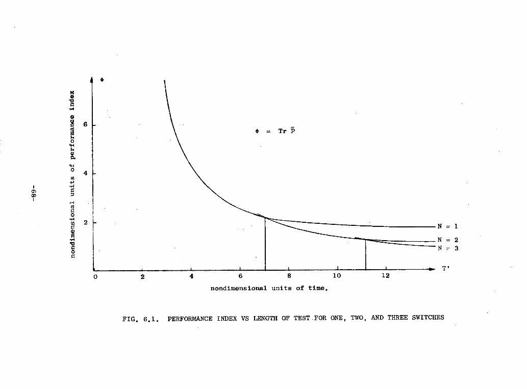
-4II
Z;
k 4ES.
.0
zz C
O
I is
4.4[..,
V
: xZ
V
o
Uo
4 .
-@mso
C
o
-4'-I
0I
xopu
Teo
uv
mu
o;ra
d S
o s4
Tun
ITuoT
suam
Tpuou
-68
-

o.
.-'
1 ~~~0
Ei~
~~
~~
~~
~~
~~
~~
~..
i.-iC
~~~~~~~~~~~~~~00
4.)
00~
~~
~~
~~
~~
~~
~~
~~
0 To
C.)I-I
O
0
am'!:.~
~o s~"!:.un T
~uo'!:~
um
'!:puoC
D
-~
a 0
-rz4~
~~
~~
~~
~~
o
a, ~
~
0
amT;q Jo
s~yu
f Tuuoyrsueluypuou
-69-

Figure 6.1 shows plots of the performance index for one switch (N = 1),
through three switches ( N = 3), for tests up to 14 time constants. For
the no-switch case (N = O), the performance index Tr P asympotically
approaches eight and is not shown but is optimal for tests under 0.2
time constants. Figure 6.2 shows the switch times.
If we were to use the suggested criterion of maximizing the trace
of I, we would have
1[ (= .1 [TS 3 2a dt
o a +
T 2 ) ]
0J
It is easy to see from Fig. 6.3 that the optimum input for this cri-
terion is a constant step u = + m, for any test length. Except for
very short tests, the constant input is the worst bang-bang input for
minimizing the covariance of the parameters!
(x)
s+I
BLOCK DIAGRAM OF STATE AND SENSITIVITYFUNCTIONS.
-70-
u
FIG. 6.3.

C. INPUT CRITERIA FROM IDENTIFICATION ALGORITHMS
Now let us look at the identification techniques of the previous
Chapter and see if they also include a clue as to an input criterion.
C-1. Quasilinearization
Refer to the summary of the quasilinearization technique in Chapter
V. During the second set of iterations, the sensitivity equations are
driven by ZN' so that the state, nominal, and sensitivity equations are
deterministic. Recall that
F = FN+ DH and G = GN + 8G
so that
aF 3D aH aG a8Gv = = qH + D F and vaa -
1 i 1 i i
so that when FN = F, GN = G, HN = H, and D = 0, the sensitivity
equation in the quasilinearization technique is equal to
= F(X)+ ()X +u ;i (to) =
Also, HN = (I-L)H
we have
so that (&L/&ai)H = (6H/6ai)(I-L) and when aN = a
·H ( I1
In such a case
tf
a = I a () R v dt
o
and its mean and covariance are given by
a= O and E T = I-
-71-
ax)3Si
ax
Ta-i (6.13)
(6.14)
(6.15)
(6.16)
a^z \TaT

However, in the algorithm, we have an iterative process that is repeated
until Ca - 0. The value of aN for which this happens is the identified
value of a. The statistics of the resulting a are not easily derived.
However, we can say that the smaller I is, the closer a is to the
true value of a.
2. Gradient Algorithm
We want to shape the input u(t)
large (therefore our gradient will be
E
ax(to)
-ax
ar(to )
axo
so that
steeper).
ax(to)a--
ar(t o)
Ha
X(to) and r(t ) will be
In fact, the matrix
is the information matrix! This may be seen by referring to Chapter II.D
and letting y denotes the augmented vector
( G) and *r
its adjoint. If i.- O, then J = J (t ) so that1 o
aJ(+)(t )ay(t )
Therefore the information matrix of
ments up through time tf is given
I(t ltf) =
_= T(t )
the state at time t0 given measure-
by
~*( t o)
y(t) · (6.17)
-72-

This is the information matrix
we want to identify x(to) and
we want for identification purposes since
a(to). If we let
\r/
then we have
I(t Itf) = Eo f
x( t o)
0
ar(to )
0
ax(to)
ar( to)
Pa
(6.18)
We can now illustrate how the information matrix may be calculated
using this indirect approach. The gradient method for the output error
criterion gives us the tWo-point boundary value problem
* = Fx + Gu,
= HTR-1(z - Hx) - FT ,
x(t ) = x
X(tf) = O
(6.19)ii = xT T R- l(-Hx) - [xT + uT -j ,
ri(tf) = 0, i = 1, 2, ... q' .
The sensitivity equations for (xT XT pT)T with respect to (xT aT)T
are given by
-73-

x- (to) = Io
(to) = 0, i = 1,2,... q'ax
'5'T
FT(/)= -F To - HTR-iH((x) -- (t) = ;o
R- (z-Hx) - HTR-1
x-i (t ) = ;
= (z - Hx)TR 1
_T F /) x \
T aHx a aH ax
_ t6 x +~ai
G )T(1 )'aX .
1 ) c -o
(6.21)
R-1axRMH
ar.2- (tf) = o ;
o
= (z - Hx) R
aF /2x \T -LJ ]a 3
(The trivial sensitivities
constant, and
X- a FaS`T
o
oaa-x
o
T aHTX a
:I
aGx + a
i
and ao
R-l[1 +[aj
uT/% \3 ,
ar.I (t3)
imply that a(t)
- 0).
-74-
= Fx )/(axx
(lJx$r/ax ) +aF
i
and
aGx + a.
1
(6.20)
ax \( 0
aFT- .
iaiFT )
(r
aHT+ ;i
i
=0
equals a
(ri
X [aI[
aH/a)x \7ia.. a-
x +H i)]
/ari H./-x )

Taking the expectation of (6.21), we have
= - FT(/ \) - HTR-1HP ) (t ) = 0 ;o ax (;f) A0
?T'6 \ T.-fa[H 1lax 1= - F ) - HR x + HV j
(:-i)(tf) = 0 i:
T aH 1H/x)- x T R- I1X a 1o
= 1, 2, ... q' ;
/aF- 3;a,
( ·(t) = 0 i = 12 2
\i T aH x -+H ax\ E / = - x v6 a L x + H( v )]
j ~~~i i
r -)(tf) = o0 i, j = 1, 2, ... q' .
To find the information matrix (before the test is run), calculate x from
(6.19), the sensitivity equations from (6.20), and the mean adjoint sensi-
tivity equations from (6.22). These latter functions at t give us theo
elements of the information matrix. This indirect method involves more
computation than the direct method illustrated in the previous section.
For the direct method, x and (0x/2ai) would have to be calculated but
then the elements of the information matrix could be calculated from quad-
ratures of the sensitivity functions. An example of the equivalence of
the direct and indirect methods of calculating the information matrix was
shown in Chapt. II.D. The example in that section may be viewed as a
parameter estimation problem for the final state x(tf).
-75-
{ax\
(ri (6.22)x + u)V (v
.3 -, 65x0
... q' ;
-aF + aG ) ,- 'Ja, k-37- .1

3. Nonlinear Filter
It might be interesting to apply one of the nonlinear filter algor-
ithms of Chapt. II.C to our problem. For this discussion, let us assume
that a represents the parameters in F and G that are known very
poorly: Paa (t ) O0; the initial state x is known quite well:aa o 0
Pxx (t ) O; we are using a canonical form where H is known and the
intensity of the process noise Q is known. By letting (a) be the
state in the extended Kalman filter, we have
x= Fx +u + P H R z-Hx)xx
a = P H R (z-Hx),ax
P = FP + Fx+Gu) pT + p T +xx xx oa xa xx
+ P ~3(Nx+8u) + Q-P HTR-1HPxa aa xx xx
P = FP + (F+Gu P - P HTR-1Hx.a xa a aa xx xa
P = -pT HTR - 1HP aa xa xa
(t o ) = xo
a(t o) = a o
P (t o ) = Po (small)
Px (to) = O
Pa (t ) = A (large)
If P (to), in addition to Pxx(to): were small, then this would
yield a reasonable estimate of the state and the unknown parameters.
However, for the problem as formulated above, we cannot integrate the
covariance equations with Px (t ) 0 O and Pa (t) C , or Pl(t ) m w and
P 1 (t ) = O. (Not to mention the premise that for their derivation, the
covariances were assumed small relative to the nonlinearities.)
-76-

Since we must have an estimate of a to design an input, we may
drop the circumflexes on F and G. Making the definitions S = P P-i~~~~~~~ ~~xa as
and I = P the last two covariance equations becomea aa
a(F +(p+Gup -p )HTR1Ils, (t)== FS + + (P p _ p ) TR-lHS S(t ) =xaaaxa xxxa
(6.24)
I = sTHTR-1 HS Ia(to) = A
-1 -1 TIf we assume that P 0O and note that I =P PP p >T0
xx xx xx xa aa xaso that o < p p-1 pT < P , we may drop the last term of the first
xa aa xa xxequation in (6.24). The ith column of S is then the sensitivity of x
with respect to ai and we have the same expression for the information
matrix as obtained by previous methods. The interesting point to note in
this approach is the interpretation of the matrix of sensitivity functions
S =P .Pxa aa
D. PROCESS NOISE
For a system with process noise, we can use the direct method of cal-
culating the information matrix since we were able to minimize (4.31) with
respect to w and obtain a Kalman filter representation of the system. For
a sufficiently long test, the identification criterion was to minimize
J 1 (z - H2)TR-l(z - HI)dt (6.25)J ( - ~ 2
t
with respect to a, subject to the constraint
x = F^x + Gu + K(z-Hx), (t0 ) = x . (6.26)
The i jth element of the information matrix is given by
-77-

a2jI -
ij -. -i j
tf T
E x i+ H)T R-IH + Hjx d t
o
(6.27)
where xi denotes ax/a.i and is given by1 1
1 ^ (~~KH)5 + KK z- )X i (F ) ii)x a ( I
ax
Xi( 0 ) =- a. -
(6.28)
Since the innovation V = z - HI, is white gaussian noise with intensity
matrix R, we may rewrite the state and ith sensitivity equations as
x = Fx + Gu + KV,
= (F- KH)xi + -K u+ u v 1 i 1 ~ La, - '5 -a ) 'Fa, \Oaac a.9
7X AThe mean of the state equation x = x, and the mean
are then gven bytivity equation . = x. are then given by1 1
Xi(t ) = x0
Xi (to) =-- .i
of the ith sensi-
x = Fx + Gu,
ki = (F-KH)xi +i i~~~~
The covariance matrix
p ij _ E(T
/6F _KaH aG- K ax + a u,
1ai
(6.30)axxi(to) = a °
PO = E(_-x)(x-x) pOi = E(. - x)(-x) and
are determined from
,Y-78-
£
(6.29)

00 00 ooT T 00P = FP +P F + KRKT P (t) = ;0
0 Fo i oi poo/FT HT T +
i (FT-HTKT) +
~KT+ T pi(t ) c=O; (6.31)
~ij ;)F )H oj ip oiFT ~HT
= <a _ K a-)P + (F-KH)P j P K T)
i)
+ pij(FT-HTKT) +T v R -v P1i(t )
i 0
Performing the expectation in (6.27) we obtain
i. S t ( H T i -1/ H1J 7-aI i )+ Tr ijHT + PjHT + Hpi HT (6.32)
aa aao
aH oo aHT R-1+Z-P P j dt
The positive definite covariances in the information matrix imply that
process noise may increase the accuracy of our estimate. However, we should
note that the new sensitivity equations (6.30) that act as constraint equa-
tions in our optimization, are also modified by the process noise. For a
simple example shown in the next Chapter, process noise tends to decrease
the effectiveness of the input, so that the net effect is a decrease of
estimation accuracy with process noise.
-79-

Chapter VII
SOLUTION FOR OPTIMAL INPUTS
A. INTRODUCTION
We have seen that a reasonable criterion for judging inputs to iden-
tify q parameters in a linear system is some measure of the information
matrix of the parameters we wish to identify. To evaluate this cri-
terion, we must solve n linear system equations which drive n .q
sensitivity equations, which, in turn are used to generate 1q(q + 1)
elements of this information matrix.
Optimization of this criterion can be formulated as a calculus-of-
variations problem (Mayer formulation) to minimize E[y(tf)] = TrDI (tf)
subject to the constraints
y = f(y) + Bu, Y(to) = Yo, Jul S m (7.1)
where y represents the state, sensitivity functions, and elements of
the information matrix. The dimension of y is then (n + 1q)(q + 1).
For the general case (with process noise), the constraints in (7.1) are
given by
x = Fx + Gu, x(t o ) = x ;
axXi(to ) = .,* (FKH) + F KaH )x+ aGii=(F-.KH)x. + -.- 'a
i~~~~I ( ai i)x+15a
(7.2)
i = 1,2,... q;
(7.3)
= H Hi/TR-1 (aH I(t) =A-1i - X + Hx x , +Cij YJii = Oa i i) 'Na7 j) + C. ij 0 ) =aa aa 1J~~~~
(7.4)
i = 1 2, ... q, j = ii + 1, ... q
-80-

where C.ij represents the second integrand in (6.32). For the case with-
out process noise, C.. and K are equal to zero.
From the linearity of u in the constraint equation (7.1),with its
absence from the performance index, and its amplitude constraint, we have,
from Pontryagin's maximum principle, that the optimal input is bang-bang
with amplitude m. All that remains is to find the switch times that
optimize the performance index.
If we let X, X. (vectors) and Xi. be adjoint variables corres-
ponding to x, xi, and Iij respectively, we can form the Hamiltonian
q
~~~~~~~~~~~q q ~~(7.5)
_jx + Hx.)R [( R x + Hx) + C ii=l j:= +c i .
The Euler-Lagrange equations for the conjugate variables are
q q q
xTF= -T - ij*T_ _ F i-'~ai - K j=i
X x + ( H aHT (-1 aH 1Xji x + Hx xR1 + x + Hx i = .- q
(7.6)
X(tf) = o
q*T T ,
X.i -i F-KH) - x + Hxj
(7.7)
- xX + HxR X 0 i 1,2 qj=i R H, ki(tf) aO- i : 1f2,... q .'5~~~~
-81-
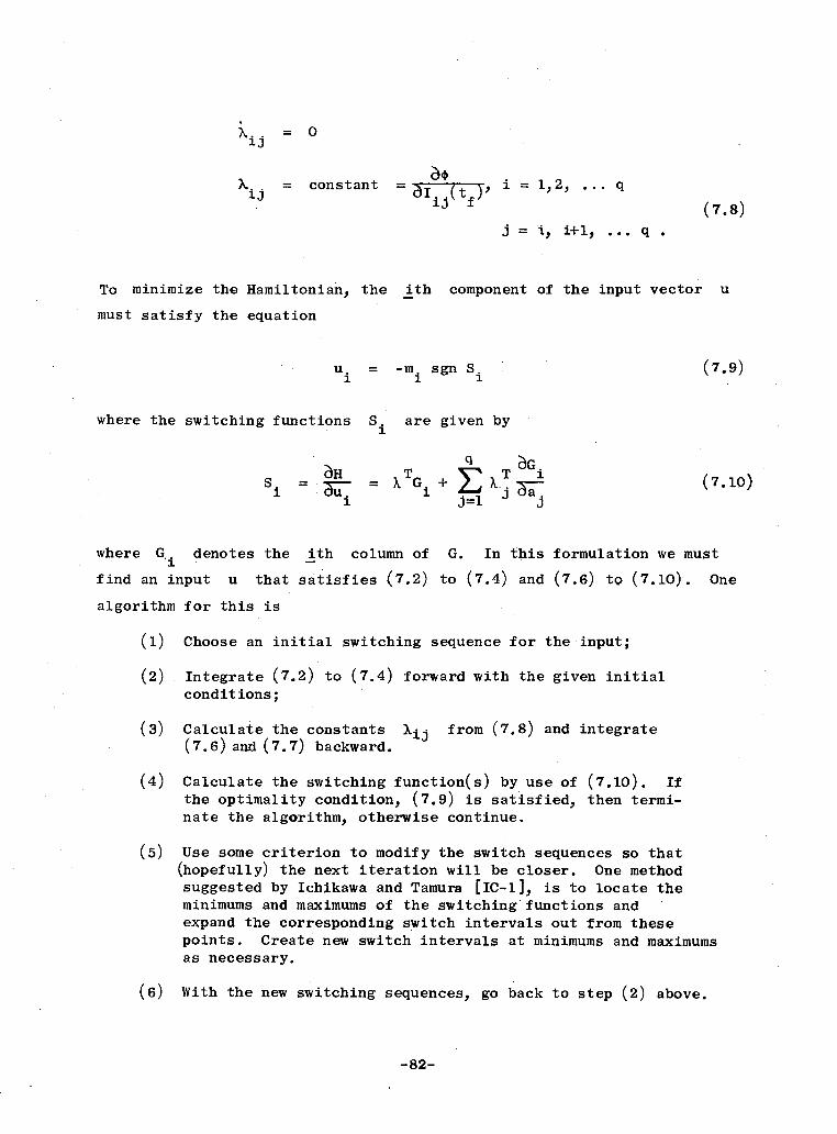
X..1J
1j
= 0
= constant = i (t), =ij f
1,2, ... q
(7.8)j = i, i+1, ... q .
To minimize the Hamiltonian, the ith component of the input vector u
must satisfy the equation
Ui = -m sgn Si1 1 1
where the switching functions
aHSi .i uu.
1
Si are given by1
q G= XTG. + X .T
j=l j
where G- denotes the ith column of G. In this
find an input u that satisfies (7.2) to (7.4) and
(7.10)
formulation we must
One
algorithm for this is
(1) Choose an initial switching sequence for the input;
(2) Integrate (7.2) to (7.4) forward with the given initialconditions;
(3) Calculate the constants .ij from (7.8) and integrate(7.6) and (7.7) backward.
(4) Calculate the switching function(s) by use ofthe optimality condition, (7.9) is satisfied,nate the algorithm, otherwise continue.
(7.10). Ifthen termi-
(5) Use some criterion to modify the switch sequences so that(hopefully) the next iteration will be closer. One methodsuggested by Ichikawa and Tamura [IC-l], is to locate theminimums and maximums of the switching functions andexpand the corresponding switch intervals out from thesepoints. Create new switch intervals at minimums and maximumsas necessary.
(6) With the new switching sequences, go back to step (2) above.
-82-
(7.9)
(7.6) to (7.10).

An analysis of the computation required shows that we must integrate
n + q . n first order differential equations and Jq(q + 1) quadratures
forward and n + q * n equations backwards for each iteration of this
algorithm. Hence, there are (q + 1)(2n + Jq) integrations per itera-
tion. This number is independent of the number of switches.
A-1. Steady-State Sine Input
For long tests the optimal input is often a bang-bang input with
almost equal switch time intervals. In this case, a good approxima-
tion to the minimum value of the performance index and the optimum switch
times can be obtained by approximating the optimal square wave by its
first (and possibly higher order) Fourier component(s). Since we are
assuming a long test time, we may use the steady-state amplitude ratio
and phase shift calculated from the transfer function. We then have
only p angular frequencies w.i i = 1,2,... p to optimize. If two in-
put frequencies are the same, then we would also have to optimize with
respect to their phase.
B. OPTIMAL INPUT ALGORITHM
Since we know that the optimal input is bang-bang, we can optimize
with respect to the switch times, tl, t2 ... tN
. To insure a global
minimum, the optimal value of the performance index may be plotted versus
the length of the test for N = O0 1, 2 ... . For example, see Fig. 7.5
of section 7.D where for T = 8, there is a minimum for N = O. 1, 2, 3.
The minimum for N = 2 is the global minimum. The algorithm of the
previous section could converge to any of the local minima. It could
not be used in the systematic method outlined above since it creates
and annihilates switch times as necessary.
The algorithm that seems most promising for determining the optimum
switch times is the conjugate gradient algorithm. Using this method, the
minimum of a quadratic function of N parameters is found in N itera-
tions. The first iteration involves searching in the steepest descent
direction until a minimum along that direction is found. On subsequent
-83-

iterations, the search is made in a conjugate direction.
The implementation of this algorithm to our problem is shown in
the flow diagram of Fig. 7.1 and follows Pierre [PI-1].
The following features concerned with the one dimensional search
have been incorporated into the algorithm:
(1) If the one-dimensional search finds a minimum at a distancegreater than three times the value of the initial step size, Althen a steepest descent search is continued;
(2) The initial Al is taken as 1/5 the initial time intervalmultiplied by the number of switch times. For a set of Niterations the same value of Al is used;
(3) For a new set of iterations, the value of Al is set equalto 1/5 the average search distances for the previous Niterations;
(4) A quadratic or cubic fit is used to find the minimum in theone dimensional search.
2. One Dimensional Search
The one dimensional search algorithm is shown in Fig. 7.2. Let r
be the direction vector in the tl through t N space given by
r = Hg (7.11)
where H is a matrix given by the conjugate gradient algorithm and g
is the gradient of the performance index. A change in the kth switch
time in the -r direction is given by
rA
t = -(7.12)k R
where N
R = E Irklk=l
Since
rk 1
R
-84-

READ and WRITE: ACCURACY PARAMETERS, AIRCRAFT PARAMETERS
NUMBER OF SWITCHES (N-1) AND LENGTH OF TEST.~~~~~~~~~~~~~~~~~~~~~~~~~~~~~~~~~
CALCULATE INITIAL SWITCH TIMES (D) AND INITIAL
VALUE OF ONE DIMENSIONAL SEARCH (AT).
SET ICNT = 0.. .~~~~~~~~~~~~~~~~~~~~~~~~~~~
I CALCULATE INITIAL VALUE OF PERFORMANCE INDEX (JO)
N=1
NO
YES
CALCULATE GRADIENT OF PERFORMANCE INDEX
WITH RESPECT TO SWITCH TIMES (PJ).
4
CNO
YES
(Contd)
FIG. 7.1 FLOW DIAGRAM OF CONJUGATE GRADIENTALGORITHM
-85-
ICNT = ICNT + 1
K = 1
AOA = 0.0
H = I
I
t #0I

PERFORM ONE DIMENSIONAL SEARCH.
STORE STEP SIZE IN AOP AND
VALUE OF PERFORMANCE INDEX IN JO
K = 1
A Ttr
AOP _ AMIN ?
YES
. NO
STORE PJ IN PJOLD
CALCULATE NEW PJ
4,I 11Pll2S SMIN ?
, NO
AOP > 3 A 1
AND ICNT = 1
AND K = 1 ?
I
WRITE JO AND
SWITCH TIMESNO
K = K+ 1
AOA = AOA + 0.2AOP/(N-1)
AT =N YES
NO
CALCULATE NEW H MATRIX
_ l .~~~~~~~~~~~~~~~~
FIG. 7.1 (Conclusion)
-86-
Al = AT
STORE D IN DOLD
CALCULATE R = - H- PJ
CALCULATE 0'(0) (PJO)i .
'04' YES
YES
I
L

YES
ISET A
2= 3A
1
INCREMENT SWITCH TIMES
A 2 - A 1 IN -R DIRECTION
CALCULATE PERFORMANCE INDEX+ P
1P< JO
5-PJO * A
NO
1CALCULATE A
2AND
DEC FOR QUADRATIC FIT
INCREMENT SWITCH TIMES
A2
- A1
IN -R DIRECTION
CALCULATE PERFORMANCE INDEX J2.,
J2
YES
CALCULATE A3 FOR CUBIC FIT1 3 I~~~~~~~~~~~~~~~~~~~~~~~~~~~~~~~l
NO
YES
JO-J2-DEC
X 0 1 DE
NOvc
NO INCREMENT SWITCH TIMES A2 - A3j3<I3< ~IN -R DIRECTION. CALCULATE J2
YES
AOP = A3 AOP = A2
JO = J3 I JO = J2
|RETURN |E N mFIG. 7.2 FLOW DIAGRAM OF ONE DIMENSIONAL SEARCH ALGORITHM
-87-
INCREMENT SWITCH TIMES BY A1
IN -R DIRECTION. CALCULATE PERFORM-
ANCE INDEX. STORE IN J1.
IF A3 > 6- A1
SET A3 = 6A 1.
INCREMENT SWITCH TIMES A3 -A 2 IN -R
DIRECTION. CALCULATE PERFORMANCE
INDEX J3

no switch time changes by more than + A,
values of the changes in switch times is
N
k=l
N
k=l,
To first-order a change in the performance
is thus
and the sum of the absolute
AA A .R
(7.13)
index in the -r direction
A T A5' = -(gl rl + g2r2+ g rN) = -r' g
2r gN R . (7.14)
In the one dimensional search portion of this algorithm, we desire to
find the value of A which minimizes the performance index in the -r
direction. * may be considered a function of A with $(0) given and
T= _ r g
R(7.15)¢' I(0)6- 1 A)__
A=O
A step of A1
is taken in the -r direction and the performance index
B(A1) is calculated. Since we have normalized our gradient, A1 may
be chosen as the maximum total expected change in the switch times, say,
1/5 the interval between switch times multiplied by the number of switch
times.
If we are sufficiently close to the optimum (so that a quadratic
fit is a good approximation), then o may be written in the form
2* = a + bA + cA (7.16)
where the constants a, b, and c are given by
a = *(0)
b = ,'(0)
O(A1 ) - ,(0) - V'(O)A1
C =2
A1
-88-

The minimum occurs at
-½ (O)A2
A b = 1 (7.18)2 =2c (A1) - 4(O) - '(O)A (7.18)1 1
Before using (7.18) as the next step size in the one dimensional search,
we should check to see if *(A1) is less than or only slightly greater
than (0O) + *'(O)A1 . Let us set an upper limit on A2
of 3A1
whenever
1 2 11(A1) _ *(0) + *'(O)A1 -6 '(O)A1 (7.19)
and proceed with a cubic fit. Whenever A2 is less than 3A1, the pre-
dicted decrease is
41 ['()A ]2
dec = (O) - pred = (A
1) - 4(O) - '(O)A1 (7.20)
If the actual decrease O(O) - *(A2) is not close to the predicted
decrease, we should go to a cubic fit. Otherwise, the quadratic approxi-
mation is sufficient for this one dimensional search.
For a cubic fit we approximate 4 by
= a + bA + cA + dA3 (7.21)
where the constants a, b, c, and d are given by
a = ,(0)
b = ,'(0)
c = e - d- A
d = (el - e2 )/(A1 - A2) (7.22)(7.22)
-89-
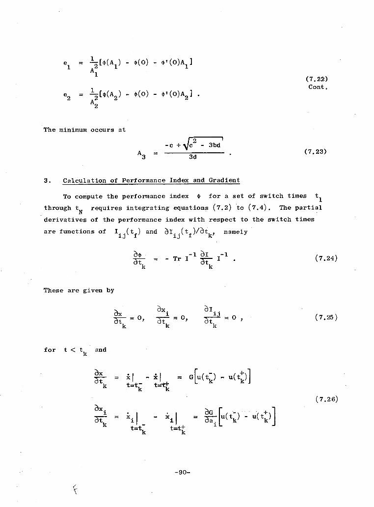
1 1 [(A1) _ (O) - V'(O)A1 ]
1 2 1 1
(7.22)Cont.
2 1 [(A2) - (0O) - *'(O)A
2 ]
A2
The minimum occurs at
-c + c - 3bd
A3 3d (7.23)
3. Calculation of Performance Index and Gradient
To compute the performance index * for a set of switch times t
through tN
requires integrating equations (7.2) to (7.4). The partial
derivatives of the performance index with respect to the switch times
are functions of I.ij(tf) and 6Iij(tf)/6tk, namely
-1 I -1= - Tr I 't I (7.24)
k k
These are given by
ax. aI..
- n = O n = (725)k k k
for t < t k and
t= o - = G[u(t). - u(tk)]k t=t- t=tkI
(7.26)
t=tk t=tk
-90-

ij) i.j| ij | (7.26)
k Cont.
t=tk t=t+k
for t = tk. For t > tk, the partial derivatives are found by solving
(t )k
. Fo E
(i ) ( a a )tk K k ) J(7.27)
Ii 6(H v x + H xi) R ( v + H )
H x + Hx jTR-f x H x j
with initial conditions at t = t k given by (7.26).
To compute the performance index involves the integration of
n + q . n first order differential equations and ½q(q + 1) quadratures.
To compute the gradient of the performance index requires integrating
( 7.27) with initial conditions given by (7.26). Since (7.27) requires
x and xi, (7.2) and (7.3) must also be integrated (unless their values
have been stored). Although this involves N (n + nq + n + nq) differ-
ential equations and Njq(q + 1) quadratures, they are not integrated
the entire length of the test. The computation involved is equivalent
to 2N(q + 1) (2n + Aq) integrations the entire length of the test.
For N > 2 this algorithm involves more computation per iteration than
the algorithm suggested in the previous section. However, it is still
used for the reason given at the beginning of this section.
-91-

C. EXAMPLE 1: ROCKET SLED TEST*
An accelerometer is modelled by the equation
y = (1 + c)u + c2 u2 (7.28)
where y is the output of the accelerometer, and u is the accelera-
tion. In order to evaluate the constants c1 and c2, the accelerometer
is mounted on a rocket sled. The sled has a maximum acceleration
ml, and can be water-braked with a maximum deceleration m2. If we assume
that the accelerometer measurement is corrupted by white noise v, with
zero mean and spectral density r, then the measurement is given by
2z = (1 + c1 )u + c 2u + v . (7.29)
The identification performance index becomes
T
o2
Since J is quadratic in c1
and c2, the likelihood equation aJ/6c = 0is linear in c1 and c2:
T
- z- (1 + Cl)U - C2 ] (-)u dt O1c 1 2
o
T (7.31)
- z - (1 + cl)u - cu2] (-)u2 dt = 0;2 o
or T T T
ioS u dt cl + u3 dt · c2 = (z - u)u dt, (7.32)
*This Example suggested by Paul Kaminski [KAM-l]
-92-
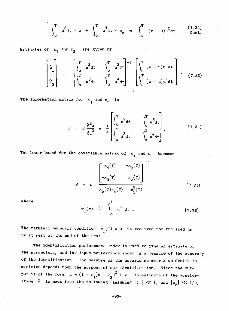
u dt 1 + udt c 2 = - u)u Cont.I~o ' "1 T To ,o
Estimates of cl and c 2 are given by
1 2~ 31· = E- ' (7.33)
o2ll tS d u dt(z u)u dt
t o (7.34)
= ~x3(T) xE (T)
x (T)x (T) - x32(T)
xt) T ; u dt . (7.36)o
be at rest at the end of the test.
The identification performance index is used to find an estimate of
the parameters, and the input performance index is a measure of the accuracy
of the identification. The measure of the covariance matrix we desire to
minimize depends upon the purpose of our identification. Since the out-
put is of the form z = (1 + ) + c2u an estimate of the acceler-
ation u is made from the following (assuming Icl << 1, and Ic2 << l/u)
-93-

- (l+^c) + l+c1 ) + 4^c2 z ^ 2u = Z - C - C2 Z
2c2
(7.37)
so that u is approximated by
= u + (c -l)u +(c2 c 2 )u +vii = 1 1 2 .2(7.38)
and the error in the corrected accelerometer output is
8U = bc1
. u cu + + . (7.39)
If the instrument is to be used at an acceleration level, a, then we
would like to minimize the error at that acceleration so that our input
performance index is given by
[ 2 : 2a a Ebc1
= tr
Ia3 a4 Ebe 5CL 3 4a c1c
2Ebc
2
= tr DP .c (7.40)
Notice that
the unknown
for this problem, the weighting matrix D is independent of
constants. Our problem then is to minimize
a x4(T) - 2a3 x3 (T) + a x2 (T)
x2(T)x4(T ) - x2(T)x2 (T)x4 (T) - x3 (T)(7.41)
subject to the constraints
x =u
2X2 = u )
3x3 = u
4x4 = u
Xl ( 0) = 0 ,
x2(0) = 0
x3(0) = 0
x 4 (o) = 0O
xl(T) = o
-94-
, = E( u)2

and
-m2 _ u 9 ml. (7-43)
The Hamiltonian for this problem is a quartic in u:
= Xu + 2 u2 + 3 u 3 + u 4 (7.44)
where
X =O or X. = constant, i = 1, 2, 3, 4 (7.45)
where (assuming a = 1),
X3(T) + x2(T)
2 (T)() - 2 2 = a negative number[x2(T)x4(T ) - x3(T)]
X3 =2x3 (T)[x2(T) + x4 (t)]
[x2 (T)x4(T) _ x3(T)] (7.46)
2 2x2 (T) + x3(T)
4 2 2 = a negative number.[x2 (T)x4 (T) - x
3(T)]
If the boundary condition xl(T) = 0 is to be satisfied, then only the
four possibilities shown in Figs. 7.3a to 7.3d are possible.
The possibility of one and only one intermediate (constant) value
m is a consequence of the Hamiltonian being a quartic function of u
(and the X coefficients being constants).
The first three possibilities shown in Figs. 7.3a through 7.3c are
considered special cases of the fourth possibility. If u equals ml
for tl seconds, -m2 seconds, and mi for t seconds, then
-95-
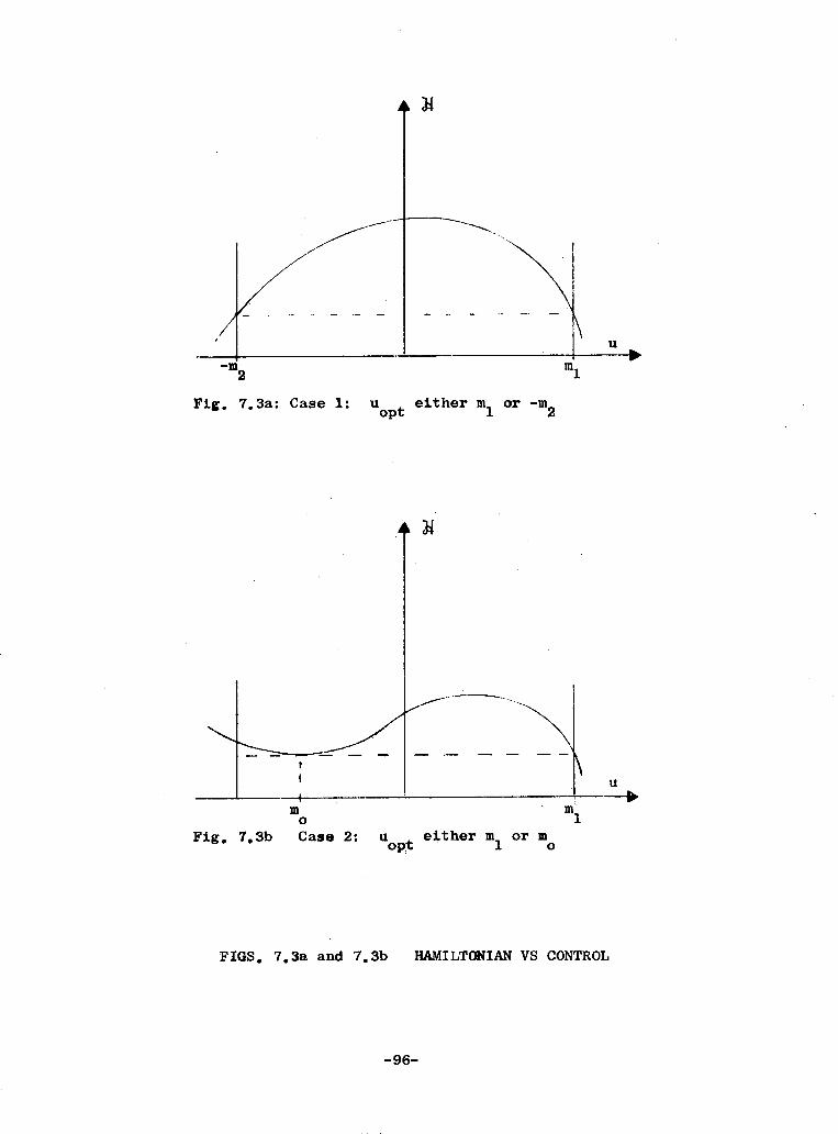
Fig. 7.3a: Case 1:
U
uopt
either m1
or -m2
Fig. 7.3b
mo
Case 2: u either m or mopt 0 o
u
m:1
FIGS. 7.3a and 7.3b HAMILTO(]IAN VS CONTROL
-96-
+ It
t

U
mo
Fig.- 7.3c. Case 3: Uopt either m or -m2opt o
x1
-m2
mo ml
Fig. 7.3d. Case 4: uopt either ml, m or -m2
FIGS. 7.3c and 7.3d HAMILTONIAN VS CONTROL (Cont)
-97-
/

The first t
T =
X 1
X =
x 2
x3 =3
4
;wo equations in
m2t -
1 mI
+ m2
m1t = _2 m1 + m
2
t1 + t2 + t o
mlt - m2t 2 + m t = O
2 2 2mI-t + m t + m tmitl m22 o00
11 2 2 0 0mltl - m2t2 + mo
m4t +m4t + m4t1 22 00o
(7.47) imply that
m
(T - t ) -0 ml + m 2 .
m
(T -t t+ 2 0 m + m2 0
The above inequalities tell
The allowable region
-m2
O
for m0
mo
!_ t
m2
t -s T0 m + m
2 o
m1
t _s T .o m
1- m°
and t is then given byo
S m1
m2
_ T for mo m 2 t m-2 o
m0 S t T for
m1m - m
1 0
0
m _ 0o
and is shown in Fig. 7.4.
-98-
(7.47)
0
0 (7.48)
us that
(7.49)
(7.50)O 0

m1
0
mo
m !_ mo 1
LMAXIMUM
mIt 2 TIo'- m2 + mn
I .t\l ' 0
I '
t o 0m-
1 IT
/o m1 0
-m 2 _ _ _
/ m - m2
FG7 ALWLRG Om2
FIG. 7.4 ALLOWABLE REGION FOR m AND to o
-99-

In summary, we are required to minimize
_2(X 4 - 2 X 3 +a 4 3T - - _2
x 2 x 4 - x 3
with respect to mA 0m = -
m1
tand t = o
T
where
x 2 -=tl +CX2 t1 2 t + m2t
3 x3 = tl-C t
3+ mt
A 4- 4x4 = t1 + C t2 + m t
t- 1t =
1 T
t2- Tt = t22
T
(c - ct - mt)c+lc + 1
= (1 - t + mt)c + 1
mA 2
C =m1
A aa = -
mAs a numerical example, let
As a numerical example, let
aa = -m1
= 0.01
(i.e., the maximum acceleration from the rocket is 100 times greater
than the designed acceleration for the accelerometer). Let us look at
two particular cases:
-100-
a x2)(7.51)

Case 1:m
2C = = 2
(i.e., the maximum braking thrust is twice the maximum rocket thrust).
Case 2:
c = 6.
For the case, c = 2, the minimum value of 0 is 0.75503 and
occurs along the three sides of the allowable region at t = 0, m = +1,
and m = -c. This means that the optimal input is u = m, for 2 T, and
u = -2m, for iT with no intermediate value of acceleration. As the
value of c is increased, a local minimum ridge forms in the region
shown in Fig. 7.4. For the case c = 6, the minimum value of 0 is
0.69127 at m = -2.7 and t = 0.2. The optimal input is then u = m1
for 0.763T, u = -6ml for 0.037T, and u = 2.7ml for 0.2T.
The foregoing Example has two interesting features: (1) the
optimal input may be designed without knowing the values of the parameters
that are to be identified, and, (2) there is the possibility of one and
only one intermediate thrust level. However, if the accelerometer is
modelled by higher order terms in (7,28), then more intermediate values
of thrust could be optimal.
D. EXAMPLE 2: A STABLE FIRST ORDER SYSTEM*
Find the optimal input to identify the parameter a in the first
order system,
= -ax + au' , x(0) = 0 . (7.53)
Z = x + v
where
Ev(t)v(t') = rS(t - t') ,
The first part of Example 2 was given in Nahi and Wallis [NA-11.
-101-
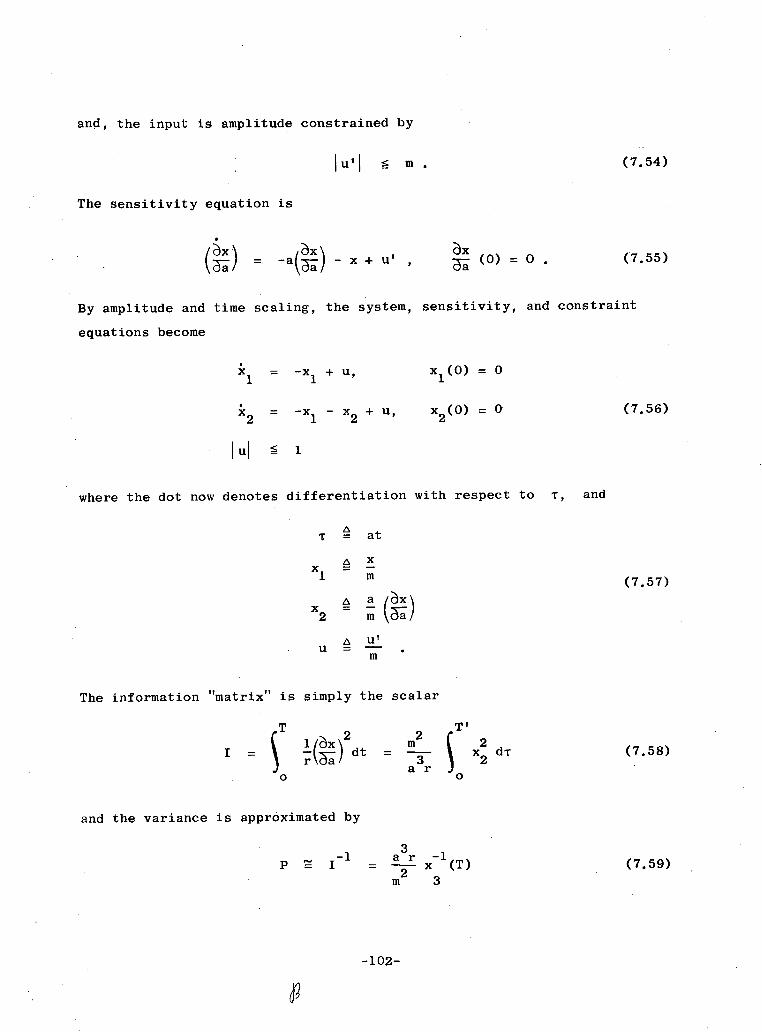
and, the input is amplitude constrained by
lu'| _ m .
The sensitivity equation is
By amplitude and time scaling, the system,
equations become
1 = -X1 + U,
2 = -xl - x2 + u,
lul : 1
where the dot now denotes
ax (0) = 0 . (7.55)
sensitivity, and constraint
x1(0) = o
x2(0) = 0
differentiation with respect to T, and
= at
A xx - m1 m
.a aXx2 - m)
A usU U'm
The information "matrix" is simply the scalar
T m )2 2
I= r a! dt=dr/ax\ 3 2r~aai 3r I x 2 dTra r0 0
(7.56)
(7.57)
(7.58)
and the variance is approximated by
P t I- 1
3a r -1
= - x (T)m 3
(7.59)
-102-
(7.54)

where2
x3 = x2' x3(0) = 0 .
The input performance index is
= P.
The gradient of 4 with respect to the kth switch time tk, is
ar -2 x3_ ~ = a r x
3(T)- -(T)
k m k
ax3(T)
k
is found by integrating (7.56) and
(a¾)\k
(7.60)
(7.61)
(7.62)
( x\ axl
k
ax2
k
/2x2(·ax33
k
(t k )
(t k )
= 2u(tk) ;
= 2u(tk) ; (7.63)
(t k ) = 0
from tk
to T.
Plots of the local minimum of the performance index for N = 0 to 3
are shown in Fig. 7.5. Figure 7.6 shows a plot of the global minimum of
the performance index superimposed on a graph of the optimal switch times.
As the length of the test increases, the center switch intervals become
approximately equal.
Since the optimal input is piecewise constant (alternatively plus and
minus one), (7.56) and (7.60) can readily be integrated from tk to tk+l to
-103-
2;x 2)z ,2 a,)_ 'X)at at at~~~'-t7t k k

0~
~~
~~
~~
~~
~~
~~
~~
~~
~0
Co
0 r>
,i k
c
o
to
-02
I I!
It II
00
LO
i,,4
It.
NI~
I
.,-4
.4
--0o
-10
4-
xep
uT
®
ourm
IoliJ
d ;o
sL
Tun
TIu
oT
suam
Tpuou

o0 '4
eaTI S
o sT
un
IsuoT
suam
Tpuou
-105-
4-.

-ak= u - [u - xl(k)]e
= x(k)e k + [u - x (k)] Zk e- ak
= x(k) + x 2 (k)(l - e-2(k) ++gk +X ()ux()[ 2~(A )
22 1+ [u x(k)[-(k)][1 - e (2tk+ 1)]
+ 4 [u - xl(k)]2[1 - e k(24 + 2Ak + 1)]
- t kk42 = tk+1
An exact (square wave) analysis assuming all the intervals are equal can
be made by using (7.64); where, for steady state it can be assumed that
xl(k + 1) = -xl(k), x2(k + 1) = -x
2(k) and they are negative for u = -1:
= -1 - (-1 - x )e-10
(7.65)
x 2 0 e + (-1 - )e-
2 ~~~10
Hence,
-A
x10 --AI + e
x 2 0
x3(T')
2(1 + e- )
= A x20 (1 e )+ -x 0 (-1-x1 0 )[l e 2(2A+1)]
+ 1 - (2}
-106-
give
xl(k + 1)
x2(k + 1)
x3(k + 1)
(7.64)
where
-x10
-x 2 0
(7.66)

Substituting for x 1 0and x20 and simplifying, we have
T'x (T') =
A(l + e )
This has a maximum of 0.213
frequency is w = 0.958.
If we had approximated
component, we would have
[1 + (1-2A)e - (+2A)e-
2 -e - 3
(7.67)
T' at A = 3.28. The corresponding angular
this square wave with its first Fourier
4u = - sin WT .
Since
x2 su 2
(s + 1)
the steady state amplitude ratio M is given by
M =1 + 21+[0
I T'
X' dT =O'
(4)2 _lW2) c sin wT dT
E (1+W2)2
A 0
8w2T'
2 2 I2(1 + w )
(7.71)
This has a maximum of 0.203 T' at W = 1.
If we take the first two Fourier components of a square wave, we
have
-107-
(7.68)
(7.69)
Thus,
x3(T') =
(7.70)

4 4u = - sin wt + - sin 3 wT
4 = w 4 3w=- + sin wT + sin (3wT + 0)
2 it 2 3ic1 + 9W2
l 1 1+ c
2 22 2 ( 4 2 9o 2
X2 = (4) X 2 sin 2T + () W2
)3 (1 3w + v -- 2 sin wT sin
i 3(l + W2)(1 +9W2
sin2 (3wT + 0)
(3wT + 0)
8w2T1 8W2T
x3(T')_= i2(1 + 2)2 +
2(1 + 9w2)2
This has a maximum of 0.211 T' at w = 0.97. The first three Fourier
components yield a maximum of 0.212 T' at w = 0.96. Taking the first,
second, or'third Fourier components yield a very good approximation to
the exact steady state solution. The computation is much simpler. In
this case, we had to optimize with respect to only one parameter, w
E. EXAMPLE 3: A STABLE FIRST ORDER SYSTEM WITH PROCESS NOISE
Find the optimal input to identify a and K in the first order
system:
x = -ax + au' + w,
Z = X + V
x(0) = 0(7.76)
where
Ew(t) w(t') = q6(t - t')
Ev(t) v(t') = r5(t - t')
and the input is amplituded constrained by lu'l [ m. The steady state
Kalman filter representation for this system is
-108-
(7.72,
(7.73)
(7.74)
(7.75)
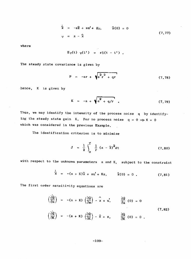
x= -ax + au'+ KV, x(0) = 0(7.77)
V = -
where
EV(t) v(t') = rS(t - t') .
The steady state covariance is given by
2 2P = -ar + Ma r + qr (7.78)
hence, K is given by
K = -a + a2 + q/r. (7.79)
Thus, we may identify the intensity of the process noise q by identify-
ing the steady state gain K. For no process noise q = 0 => K = 0
which was considered in the previous Example.
The identification criterion is to minimize
21 I 1 (z -r )2 dt (7.80)0
with respect to the unknown parameters a and K, subject to the constraint
x = -(a + K)^ + au'+ Kz, x(0) = 0 . (7.81)
The first order sensitivity equations are
() == -(a + K) -x + u, (0) =
(7.82)
I) = -(a + K) ) - x + Z (0) = TK_~~~~~~~ (0) = 0
-109-

The information matrix for a and K is
TT 2,·
E x2
x dtS E x 2 dt
I = Ir
.T
E x2x3 dt
Xl = -axl + au + KV,
= -(a + K)x2
- x1 + u,
X3 = -(a + K)x 3 + V,
Let x = x + 5x so that
0
-(a+K)
0
0
0
- (a+K)
-a 0
-1 -(a+K)
O 0
X1
R2
x 3
0
0
- ( a+K)
+
-110-
where
T
soE x3 dt
(7.83)
X1(0) = o
x (O) = 02
x (O) = 0 .3
(7.84)
x1
X2
x3
-a
-1
0
a
1
0
U',
xl(o) = 0
R2(0) = 0
X3(0) = 0
and
(7.85)
1
2
8i3
5x1
5 x2
8x 3
+
K
0
1
(7.86)
I T
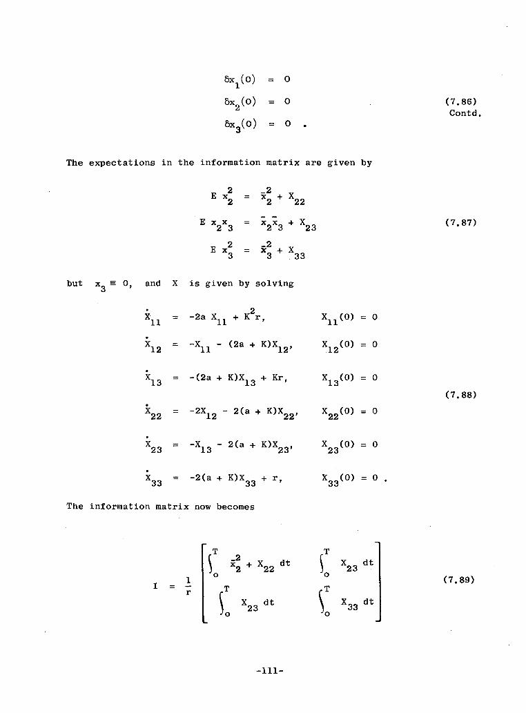
x1(0) = o
8x2 (O) = O (7.86)Contd.
8x3 (0) = 0
The expectations in the information matrix are given by
2 _2E2 x2 + X22
E x2x3 =23 (7.87)
2 -23= 3 + X33
but x3 O0, and X is given by solving
X = -2a X + K2r, Xll(0) = 0
X2 = -Xll - (2a + K)X1 2 , X1 2 (0) = 0
=13 = -(2a + K)X13 + Kr, X13 (0) = 0
(7.88)
22 = -2X1 2 - 2(a + K)X2 2, X22(0) = O
23 = -X13 -2(a + K)X23 ' X23 (0) = 0
X33 = -2(a + K)X33 + r, X33(0) = 0 .
The information matrix now becomes
T 2T
2 + X 2 2 d X2 3 dto o1 (7.89)
I T T
so X2 3
dt33 dto o
-111-

where for long tests, the covariance elements are approximately constant,
so that
T
so
T
so
K2rT22
d t2a(2a + K)(a +K)
X23dt
T
o X33dt
-KrT2(2a + K)(a + K) (7.90)
rT2(a + K)
The lower bound of
P= r
the covariance matrix for a and K
T
0X33 dt
5i X23 dt0
T
0X23 dt
X2 2 dt +
T
o
jT
o
The optimal input to minimize the variance of a and/or K is found by
maximizing
T -2'x2 dt
or minimizing
subject to the constraints
1
d TS ,R dt
o
-112-
is
(7.91)x2 dt2
(7.92)

x I= -a1 + au',1 1 I
x2 -X1 - (a + K)i2 + u',
X1 (0) = 0
X2(0) = O
lu' I m .
This reduces to the case without process noise if K is set equal to
zero,
The optimal input continues to be bang-bang, but the switch times
are changed by the addition of process noise. Normalizing the constraint
equations, we have
X1 = -X1 +
x2
= -X1
- X 2+ U,
X1(0) = 0
x2 () = 0 (7.94)
lul _ 1
where the dot now denotes differentiation with respect to T, and
T _ at
A X1x = _1 m
A a _x = - x2 m 2
A u'u = _
m
(7.95)
a+ K1 =
a
The problem may now be solved as in the previous Example for differ-
ent values of i. The performance index ~, is shown vs the test length
for various values of ~ in Figs. 7.7 through 7.9. As the process noise
increases, the switch intervals become shorter and the effectiveness of
the input is reduced. Figure 7.10 shows the performance index and switch
times for r = 2.
-113
(7.93)
= qa1 + 2rJFa r

II ii
I. Ii
z zz
00
E-4II
Ic~~
~~
~~
~~
~~
~~
~~
~~
~~
~~
~~
~~
~~
~~
~~
i~
~ ~ ~ ~ ~ ~ ~ -
II
0
P4
F:
"os
DI
C4
LO
r-
4
r.c, q
+~
~~
~~
~~
0:
*r
,II
I-0
cq
-11
4-
xapu
T
aouu
amo;aed
So
sjTu
n
leuo
Tsu
amT
pu
ou
m

II II
II
z z zo
Imi4
0
E
3m
t~~
*
X rzl
p4
C')
p.'
________ 0~
~~
~~
t
-115-
P4
m C
d O
11 II
p4
'II
Uto v
Co) C
xep
uT
aouum
iole
d
So
s;Tu
n
IruoT
suam
Tpuou

II II
il II
II
--+· p
p
X-IP
e ~ ~ ~ ~ ~ ~
~ ~
~~
~~
~~
4
-4
art I
·re~~~~~~~~~~~~~~~~~~~~~~~~~~~~~~.
I-
F n +lo~~~~~~~~~~~~~~-
p.. ~~ ~
~ ~
~ ~
r *
a a
0~~
~~
~~
~~
~~
~~
~~
~~
~~
~~
~~
~~
~~
~~
~·e
-11
6-
xepuT eo
uaem
ao
jed
;o
s4T
un
ruoT
suoumT
puou

00
//4 r z4e
F~
~~
~, ~
~ i
,~ I,
~~~~"s C
"~~~~~~~~~~a
0
~~
~~
~8 ,
.r
t- P
.~~~~~~~E
CO
*145,
/~~
~~
~~
~~
Ii
t'qr-4JP
II~~
~~
~~
~~
~~
~~
~~
~,1
,I
G'!::i
so
9::.'!u
n
'[uo'!:u
al~
pU
uo
r. &
~~
~~
~~
~~
~~
~~
~U
*
·rl~~
~~
~~
~~
~l
p4
/~~
~~
~~
~0
j 0~~~~~~~-~~~~--7-
d~
~~
~~
~~
-
-~~
~~
~~
~~
~~
Frz
~~~ N~-
4J~
~~
~~
~~
~~
~~
~~
~~
~~
~~
~~
~~
Z
ao co
or~~~~~~~~~~~~j
GU
C?
jo
s7~
uf
TUuoysaUGUIpuou
-11
7-
pm
~C'

For long tests, we can show that the increased information from the
covariance term is not sufficient to compensate for the lost effective-
ness of the input (except where the deterministic input is severely con-
strained). For a long test, let us approximate the input with
4U = - sin oT .
xx2 su (s + 1)(s + 1)
(7.96)
(7.97)
the steady state amplitude ratio M is given by
M = (1 + 2)(2 + 2)8 (1 +U ) 2 + W2 )I
(7.98)
andx2 dT (422dT = (-)
T'
o
2C 1
1 T'
(1+ W22(~2+ 22
This has a maximum of
8T'
i (1 + 1)2
at C = i .
If K is known, the covariance of a is
T
r ~ X33dto 3
[; . X2 2 dt + I x22dt . I X3 3 dt - I X2 3 dt]0 )O j O L0
For long tests, the inverse of the covariance of a is
-118-
Since
(7.99)
(7.100)

1 m 8T' 1221 8T' (7.101)
a r 2 ( + 1) 2a (2 + 1)
If we let
a 21 and m2 mar a
then, [ 2 + +6 1 ( 2
1 T It (7.102)
O' 2a2 + 1 )2
A plot of this function is shown in Fig. 7.11 for different values of B.
From this figure, we can see that a little process noise usually degrades
the overall accuracy of identification. However, where the input u is
restricted to small values (I small), a larger amount of process noise can
increase accuracy.
To get an idea of a reasonable amount of process noise compared with
the deterministic input, let us assume that the process noise could be
generated through the input u, w = au, and that we constrain the
variance of u so that 3a equals the magnitude of the inequality con-
straint:
ama aao 5 - (7.103)w u 3
If the correlation time is A, then
22q = 24a 2 m (7.104)
In terms of a and P this inequality becomes
22a q 2gaa m 2~a 2
a 2 2pam = 2-a P2 (7.105)2 2
a r 9a r 9
so that a realistic a in Fig. 7.11 is very small and would only degrade
the overall identification accuracy.
-119-

<11
GII:
oll
qcj
to 8
°3104d-ra
r. o 0
0a I
cq 0r 4
'-4
-12
0-
0II
IQ.
0lIC
;
tor.1itHn
UO
BO
UT
- tu
n
UOTSUTPUOU-o
~v
a
uoT~vou1i-o
Xo
S4Tun
luuoTsuaempuou
0

F. EXAMPLE 4: A STABLE FIRST ORDER SYSTEM WITHA STATE INEQUALITY CONSTRAINT
Solve the problem in section 7.D with the addition of a state con-
straint
lxI s a m . (7.106)
For a 1 this
region Ixl [ m,
trol constrained
constraint has no effect since x is always within the
for lul s m. The optimal solution is made up of con-
arcs (u' = + m) and state constrained arcs (x = + am).
The scaled equations are
X1 = -X 1 + u
2 = -x 2 - X 1 + u,
2
X3 = x2 '
uI 5u 1,
Ilx1i a,
The time, ta,
1 (0) = 0
x2
(0) = 0
x3(0) = 0
0 < a <
needed to get to the state constrained arc is given
by
t = -n if u = +1a 1 - x
(7.108)1 -a
t = -n if u = -1a 1 -x
Let us define the switch times as the time when the control, u goes to
+ 1. If the interval between switch times is greater than t , then wea
follow a constrained arc for a portion of the time between switch times,
A typical input and output sequence is shown in Fig. 7.12. The problem
may be solved as before with the addition that if the kth switch time
is greater than tk_l + ta, then the control u is set equal to ± 1
from tk-1 to tk-1 + t and set equal to ± a from t + t to tk.k-i k-l a a k-l k
-121-
(7.107)

U, X 1
-1
u
x1
FIG. 7.12. INPUT AND OUTPUT CURVES WITH A STATE
INEQUALITY CONSTRAINT.
This problem has been solved for a = 1 and is shown in Fig. 7.13. A
comparison with Fig. 7.6 shows that the switch times are closer together
than the case without a state constraint. As before, the first and last
switch intervals are smaller than the central intervals and the central
intervals are approximately equal.
Now let us see how the steady state solution is modified by the
state inequality constraint. Recall that without a state-inequality
constraint, the steady state solution yielded a time between switches of
3.28 time units, and that the maximum deviation in x was given by
-3.28ax1 = -3.28= 0.929 (7.109)
l+e
so that for a 2 0.929, the steady solution is already solved with
1 4.700.213T' T'
For a < 0.929, we must allow for a portion of each switch interval to
be on a state constrained arc.
Let us define t as the time between switches on a control con-c
strained arc, and t the time on the state constraint. If we start
Sl n 719
-122-

01cVIKK
vl~
~~
~~
4
a\ \
E
r~~
~~
~'
o
am~ ~o s~un ~uo~suem
~puou0
'-4
w
~ ~
~ ~
~ ~
~ ~
~ ~
~~
o~
~~
~~~~ ~~~zO
-4i
'-4
CO
~~~~~~~~~~~~~~~~~~~~~~~~~~~~~-
0'0 A
1-4
~~
~~
~~
~~
~~
~~
~~
~~
~~
~~
~~
~~
~~
~~
~~
~~
~~
~~
~~
~~
~~
~~
~E
4E
4a
o~~~~~~z
/~~
r 0
FG
~~
~~
~~
~~
~~
~~
V
-4
/~~
~~
~~
~~
O~
~~
0C
Go v9
cq
eurj; So slrun EvuoTsuemlpuou
-12
3-

at x1(0) = -a and x2(0) = -I with u = +1, then at t we have
-t cx(tc) a = (-a - l)e + 1
(7.110)
-tc tcx(tc) = -e - (-a - 1)t e2 c c
On the state constrained arc x a so that at t + t1 s s
xl(t + t) = a
1 c s (7.111)-ts
x (t + t ) = = x (t )e2 c s 2 c
The value of t and P is then
*ct = -£n -
c 1 + a((7.112)
-t s(1 - a)t e
c
1 - -ts1 +
The total increase in x3 during this time is A + A where A
is the increase of x 3 on the control constrained arc, and A is
the increase on the state constrained arc. A and A are given byc s
ac= 2 (1 - 2 te 1 2tc-P2 (1 e-2t) + - M(--) e - e (2t + 1)c 2 2 [i c
+ ( + 1)2[ - e ( 2 t +2 t +1) (7.113)4 c C (7.113)
1 2 -2tsAs = -x(t )(1 - e )
s 22c
The normalized covariance is then 4' = (t + t )/(A + A )T'.
For a given value of a, this can be minimized with respect to t .s
A plot of t, t + t and 8' T' is shown in Fig. 7.14 for a = 0.05
to 1.0. As a becomes smaller, the covariance increases and the switch
intervals become smaller.
-124-

4:
m
o~
~~
~~
~~
~~
~~
~~
~~
~~
~~
~~
~~
f
c, C
,~~
~~
~~
~~
~~
~C
.4.)~
~~
~~
~~
~~
~~
~--HVI
Ea
Cd
10 -4
f-I-
II ~
~~
~
~ r
mci
am
4
os4u
InuosumE
uo
cr) CT ~
~ ~
~ ~
~ C)
-
&I
*sd
JO
s4T
un
IruoY
suem
-rpu
0
-'-I
n-4
E-e
~~
~~
~~
~~
~~
~~
~~
~~
~~
~~
~~
~~
~~
~~
~~
~~
-
re~
~~
~~
x
GW
y~
J0 sITun
~euoysu91Tpuou
rJ %rd ~o
s~ruf V3uoTsuQIUTpuou
-125-
x
o4J

The interesting feature of this Example is the fact that the state
does stay on a state constraint for a portion of each cycle, and the
frequency of switching is increased.
G. EXAMPLE 5: AN UNSTABLE FIRST ORDER SYSTEM
Find the optimal input to identify the parameter a in the unstable
system
= ax + au, x(O) = O, a> 0(7.114)
Z = + V
The sensitivity equation is
) = a() + x + u (7.115)
If the only constraint is the input amplitude constraint lul • m,
then the optimal input is u'= ±m with no switching. To maximize
T
we desire the largest possible x and u' terms driving the sensitivity
equation. If u'= ± m, then the input from u' and the input from x
are as large (in absolute values) as possible. For this Example, whenever
x is outside the region lxI < m, then the system cannot be controlled
by an input whose amplitude is constrained by I|ll s m. For this reason
we may wish to add a state variable inequality constraint
lXI a m (7.116)
where 0 < a < .
-126-

The optimal input is made up of state constrained arcs (d' = + a m,
x = ± a m) and control constrained arcs (u' = i m when Ixi 5 a m). By
amplitude and time scaling, we have
Xl = X1 + u,
X2 = 2= 2 1 + U,
= 2x3 = x2
Iul _ 1
x1(0) = x1 0
x2(0) = 0
x3(0) = O
(7.117)
l xi X1 a
where the dot now denotes differentiation with respect to T, and
T = at
A X1 m
2 - )
.=UVm = -m
The information "matrix" is the scalar
T 2 T'
I = ()2d =
0 0
221 2m / 2 1 2(-a) X2 a = 3 x3(T')
a(7.118)
so that the variance is
3a -1
P - 2 x3 (T') , (7.119)m
On a control constrained arc (u = + 1), the solution to (7.117) is given
by
-127-

x (T) = (x10 + u)eT - u1 10
x2
(T) = x2 0eT + (x + u)TeT
1 2 2Tx3(T) = x3 0 + 2 X20(1 +e ) ~~~3 30 ~~~~~2 ~20 (7.120)
1 2 T+ x20(xlo + u)[1 + e2 (2T-1)]
+ (x 2 2 + 1) - 1]
and on a state constrained arc (xl = x10), the solution to (7.117) is
given by
X1(T) = x10
TX (T) =x e20 (7.121)2. 20
(T) 1 2 (e 2T)X3 () = x3 0 + x20 (1 +
Let us now evaluate the performance index along two paths. The
first path is u = sgn x(O) until the state constraint is hit and then
to stay on the state constraint. The second path is u = -sgn x(O) until
the other state constraint is hit and then to stay on that state constraint.
Along path 1 we have
x1 () (x1 + l)eT - 1
x2(T) = (x1 0 + 1)Ter (7.122)
x3(T) 1= 2(x + 1)[e ( 2t - 1
x (r) = 1(x + 1) L a2 - 2T + 1)- 1],3 4 10~~~~~~
-128-

for O _ T - T i and
xl(7) = a
1
2 ( ( 4101
1 2 2 2+ 2(X10 + 1) ie El + e
for T 2 91, where T1 is given by
T1 = n 1+ 1 1+ x10
Along path 2 we have
X1(T) = (x10 - 1)e + 1
x2(T) = (x10 - 1)- e
x (T) = 4 (X - 1) [e (2T2 - 2T + 1) - 1]3 4 10
for O < T T and2
x1 (T) = -a
x2(T) = (x10- 1)2e2 10 2
x3(r) = 4(x - 1) [e 2 (2T2
- 2T2
+ 1) - 1]
1 - 2 2 2 T 2 ( + e T2)+2 10 2e
for T 2 T2, where T2 is given by
-129-
(7 123)
(7.124)
(7.125)
(7.126)

1+¢
1 - X10
It can be verified that x3(T 1) along path 1 is greater than x 3(T)
along path 2. However, it can also be verified that [x2(T
2)1 along
path 2 is greater than [x2(T2)I along path 1. This means that if
x3(T2
) along path 2 is not greater than x3(T2) along path 1, it will be
at some later time. Let us designate T3 as the time at which X3(T 3 )
along both paths are equal. Also consider that once on a state constrained
arc (with a sufficient magnitude for x2), it is better to stay on that
arc than go to the other constraint or go off and return to that arc.
For these reasons, we can say that the optimal input is u = m sgn x0
until the state constraint is hit and then is such as to stay on the
constrained arc, for a test whose length is less than T3. However, for
a test whose length is greater than T 3 , the optimal input is u =
-m sgn x until the opposite constrained arc is hit and then is such as
to stay on that constrained arc. However, in both cases, the optimal
input involves going to a constrained arc and staying on the constraint.
This Example has two interesting features: (1) Since the state and
sensitivity equations are unstable, the information matrix grows much
faster than for a stable system. This means that an unstable system may
be identified more accurately than a stable system. (2) The optimal
input involves no switching.
H. EXAMPLE 6: AN UNSTABLE FIRST ORDER SYSTEM WITH TWO PARAMETERS
Find the optimal input to identify a and b of the first order
system
= ax + bu', x(0) = 0, a > 0(7.128)
Z = X + v
with an input amplitude constraint Iu't < m. The two sensitivity equa-
tions are
-130-

(x)
rx)rixs
and the information matrix is
= a(t) + x
= adze" + u!
I
By amplitude and time
1 lT ( )2
r T | dt
scaling, we have
scaling, we have
Xl = X1 + u,
x2 = x 2 + X1'
x3 = x3 + u,
lul 1
TT /) x x)
d t
| (8) dt
i~x.o~s;I
x1(0) = 0
x2(0) = 0
x3(0) = 0
where a dot now denotes differentiation with respect to T, and
T = at
a
a2x
X2 = b3
x3 m ;a- b
-131-
(7.129)
(7.130)
(7.131)
(7.132)
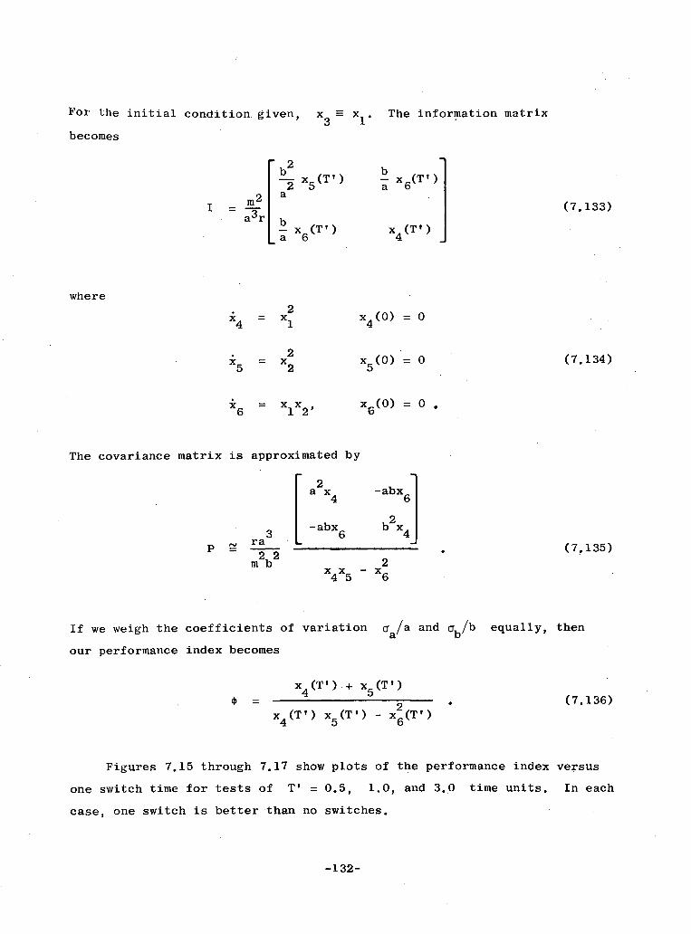
For the initial condition given, x -3
becomes
I =ar 6
where2
x4 = Xl
25 2
x5 = x26 1 2'
x1. The information matrix
b- x (T')a 6
x4(T') I
x4(0) = 0
x 5(0) =
x6(0) = O .
The covariance matrix is approximated by
2a x
44
3ra
m2b2
-abx6
-abx61
b2x4Jb 4 j
(7. 135)2
x4x5 - X6
If we weigh the coefficients of variation a /a and ab/b equally, then
our performance index becomes
x4(T').+ x (T')
2x4(T') x5 (T') - x6 (T')
Figures 7.15 through 7.17 show plots of the performance index versus
one switch time for tests of T' = 0.5, 1.0, and 3.0 time units. In each
case, one switch is better than no switches.
-132-
(7.133)
(7.134)
(7.136)

>,
4-).HC
a
0 -)
>
Ca o
0
*X
H
I,
\· .r4
0
!d o
\d 0
>
.H
0 0z
=Ic
C
OI 0
0C;
o o
oo
0 0
o 0
0
xapu- aoueujo
~la
d Fo
s4T
un
TvuoT
suam
Tpuou
-13
3-
_"

) 4
1 -H a M
~
ar
XC
r
0k~
~0
r
ImI
Do o
/ ·
, t
ow
fr
o .
x0
at ~ ~
~ oo
c
l~~
~~
~~
~~
~~
~m
' o
-o
1-4
tI
I 0
0 0
0
-134-
G). I
~cd
.4)
4 et
o0
0pu o
un
uopuou
xapuT gounmao;aad So s;lun TvuoTsuamTPUoU

.4.)
4-)~
~~
~~
~~
~~
~~
~~
~~
~-
4r~.) ~
~
M~
~~
~~
~~0
4eou
4o 0
cN
.~~~~~~~~~~4 ~ ~
~ .
m~
~~
~~
~~
~~
~v
>4
X-4-I
02C
d ~~~~~~~~-p
-4 4-)~
~~
~~
~~
~~
~~
~~
~~
~-
0J
o
x0puT
oT0
, 1
1 0
-rJo 0r
x Q
ulaovmo
edjo
s4un
uo
ua·p
o
H
·rl~~
~~
~~
~~
~~
~f
0
c, .I
I CIf)0
0
t *I
*,
* 0
w
I m~~~~
xepu~~~~
e~~~u~~nu~~~o~~Jed ;o
s~~~~~~un T~~~~uo~~suew~~~~puoucr
-135-

Plots of the performance index versus two switch times were also
run. However, in each case the best two-switch sequence was the one-
switch case. For this reason, it is believed that the optimal input is
bang-bang with one and only one switch. This is in marked constrast with
our stable systems that involve repeated switching for long tests.
Now let us solve the problem with the first order state-inequality
constraint
bmIxl aaa
where 0 < a< 1
As in the previous Example (G), the optimal input is made up of
state constrained
bmx =+ a-
a
and control constrained
u' = + m
arcs.
In mechanizing a program to calculate the performance index as a
function of the switch times, the switch times are defined as the times
when the control u goes to +1 or to -1 (not when it goes to some
intermediate value to stay on a state constraint).
Figures 7.15 through 7.17 also show plots of the performance index
for the case a = 0.9. As in the case without a state inequality con-
straint, one and only one switch is optimal. This example is quite similar
to the previous unstable system. The main difference is that to identify
two parameters, the optimal input involved one and only one switch.
-136-

Chapter VIII
OPTIMAL INPUT FOR THE IDENTIFICATION OF THE LONGITUDINAL
DYNAMIC STABILITY DERIVATIVES
A. PROBLEM FORMULATION
The approximate longitudinal equations of motion (short-period os-
cillation) for an airplane are*
M- + M (z M (Ma Mbq_ Ma q Mq + _ + + -
Iy ymuo y \I mu e
(8.1)z ze
a q+ za a + z5mu mu e
o o
where
q = pitch rate
a = angle of attack
eelevator deflection.
Let us assume that all the parameters except
mined from wind tunnel tests. Hence, we wish
parameters
M. and M can be deter-a qto identify the normalized
Ma M
Pi = I and P2 - IY Y
from a flight test.
This form of the equations was taken from Denery [DE-1]
-137-

For this test, let us assume that the only measurement is the pitch
rate q, which is corrupted by white gaussian noise of density R (a
scalar). Our problem is to determine the optimal input 8 for the
identification test with the constraint
1 e1 8 emax (8.2)
The identification performance index is
(z - q)2 dt (8.3)
so that the information matrix is
I =a R
¶: ( fdt
o k1 v) k7ZIo lo dt
(8.4)
If we approximate the covariance matrix for P1 and P2 by Ia - and
put an equal weighting on their accuracy, our input performance index
becomes
-I= Tr I (8.5)a
In order to evaluate the information matrix, we must calculate the
two sets of sensitivity equations
Md + M /{ \
Iy \pl/
+ Z 6e'mu e
+( + -i +q+ a Iymuo Iyp muYoY'~~, o
aq
a1(0) = ;
-138-
(8.6)
j = 1 To

= mu( )(0) = 0
apl(8.6)cont.
M. + M. +Mz
I P I mu I op2y 2 3 y
q (0) = 0
ap 2
-p (o) = 02'P
__ (q + Zo /C ,tE} omu2
B. NORMALIZATION
The state,
in the form:
sensitivity, and constraint equations may also be written
q = k32q + k34 + g31 e,
a = q + k54a ,
&(1) = q(l) + k 5 4 (l),
(2) = 3 2 q(2) + k 3 4 a() + qk,
&(2) = q(2) + k54 (2),
q(O) = 0
a(o) = O
q(l)(O) =
a(l)(o) =
q(2)(0) =
a2)(o) =
0
0
0
0
O
O
I el - 5emax ,
where the ith superscript denotes the sensitivity equation for Pi
The correspondence between old and new coefficients is shown in Table
8.1. k3 2 and k34 are unknown and bg3 1and k5 4
are known from wind
tunnel testing. By amplitude and time scaling, we can reduce the
above set of equations to the form:
-139-
a \\a-P
(%)2
(;)(8.7)
(8.8)

Table 8.1
RELATIONSHIP BETWEEN COEFFICIENTS IN (8.1) and (8.8).
The numerical values are those in [DE-1] for the C-8
airplane in a landing configuration. We assume that
some parameters are known or unknown from wind tunneltesting.
M. z
I muy o
azeI mu
y o
M+Ia
y
Mbe
I
k32
Old New Numerical Known or
Coefficients Coefficients Values Unknown
M. + Ma qI
Y
k34
8g 3 1
zamu
Zbe
muo
8g 51
-1.588
-0.562
-1.658
-1. 737
0.005
unknown
unknown
known (if 8g5 1 = 0)
known
assume = 0
-140-
I-
I
I

x1 = -ClX - C
X2 = X1 - X2 '
3 = -clX3 - c
X4 = X3 - x4
x5 = -cLX5 - c
x 6 = x5 - x 6 '
Jul : 1,
where the dot denotes
2X 2 + u ,
C2X 4 + X1 - X2 5
C2x6 + x ,
x1 (o)
x 2 (o)
x3(0)
x 4 (o)
x (o)
x6(o)
= 0
= 0
= 0
= 0
= 0
= 0
(8.9)
differentiation with respect to T = -k5 4 t, and
x A _ -k54x1 =
g31 emax
2
A k54x a
2
A 54 (1)
5 3 1 · 5 emax
a -k54 .~
4 6931 ·emax
2
A k5 4 (2)= q
31 emax
3
a -k 54 a(2)x =6 = g 5
931 emax
6e
u emax
k32C
1 k54
-k
c2 =7--k 54
-141-

In terms of the normalized variables, the information matrix becomes
2 2
g31 emaxI =
a 5Rk
5 4
5T'
Jox3ds 50 3x 5 dx d
x3x5d¶2
I T'xd
(8.10)
where T' is the length of the test in normalized units of time. The
input performance index is then
-Rk54O = '2 2
93 1 emax
x7(T') + x8 (T')
'tt = - .2
x7(T')x8 (T') - x9 (T')
where
2x 7 = x 5
2X8 = x
3
x9
= X3X5
The evaluation of
(2 state equations, 4
length of the test.
x7(0) = 0
x 8 (O) = 0 (8.13)
x 9 (O) = 0 .
* for a given input requires nine integrations
sensitivity equations, and 3 quadratures) the
B.1 Gradient of the Performance Index
To calculate the gradient of the input performance index we must
calculate axi/6tk for i = 1, 2, ... 9. For t < tk' we have
ax.
7 -t = 0,k
i = 1, 2... 9.
-142-
and
(8.11)
(8.12)
(8.14)

At t = t we havek
ax.1tk
= i -
t=tk- xii+
t=tk
i = 1,2,... 9
which equals zero except for i = 1 which is
ax kt =u(tk) - u(tk) = + 2
(8.15)
(8.15)'
For t > tk, we must integrate a set of 15 differential equations. The
first six equations are given by (8.9) with the values they had at t = tk
as initial conditions. The last nine equations (with initial conditions
given above) are:
x 7 = -Clx7 - c2x8
X8 = x7-x 8
= -x - c2x10 + X7 - x 819 210 7 8,~~~~~~~~~~~~~~~~~~~~.
= x9 - x10
x7(tk) = + 2
x8 (tk) =
x 9 (tk) =
Xio(tk) =
=-Cx - c2x12 + X7
= x1 1
- x12
= 2x5
x 1 1
= 2x 3x 939
= x3 *xll + X5X9
X15 (tk) =
where x7 through x15 designate axl/6tk
through axg/atk
. The gradient
of the input performance index with respect to the kth switch time is
then
-143-
0
0
0
11
x12
x 1 3
x 14
xll(tk) =
X12(tk) =
X13 (tk)
0
0
= 0
= 0x 1 4 (tk)
O ;
X9
10
x15

a', x1 3 (T') + x14 (T') [x7 (T') + x8 (T')]
=at ~~~~~~~2k D D
X [x1 3(T') xT') + x7 (T')xl4(T') - 2xg(T')x1 5 (T')]
2where D = x7(T') x (T') x- x(T')
A computer program for the optimal inputs is shown in Appendix A.
C. RESULTS
For one switch (N = 1), a plot of V' was made versus tl for
various test lengths, namely, T'= 1, 3, 5, and 10 time units. These
are plotted in Figs. 8.1a through 8.1d. For the first three cases, there
was only one central minimum. For the last case, we see two local minima,
the one on the left being the lower. Since the inverted plateau of this
latter case is quite long (and the performance therefore rather insensi-
tive to changes in the switch time), we might suspect that only one
switch is not a global minimum for T' = 10 time units.
For each of the figures 8.1a through 8.1d, there was also a local
minimum at t1 = O. This corresponds to the N = 0 case (i.e., no switches).
In general, we may say that for the N switch case, there is a local
minimum corresponding to the N-1 case. In using the algorithm developed
in the previous Chapter, our initial values of the switch times are near
the center, so that we converge to a central minimum.
A plot was made of ~' for the optimal switch times for N = 0
through N = 3 and is shown in Fig. 8.2. The lowest value of ' from
this curve and the switch times are shown in Fig.8.3. This, then, is the
solution curve. For example, if we wanted to know what the optimal input
is for a 10 sec test, we would look under T' = -k5 4 *10 = 7.37 time
units. At this test length, t = 3.00, t2 = 6.18, and ' = 61. In
other words, the optimal input is full elevator on for 4.07 sec, then
full elevator on in opposite direction for 4.31 sec, and then full elevator
on in the original direction for 1.62 secs.
-144-

0
1500
X |T' 1.0
'C 100. 3
., 100\
o'
50
0 t'
c4
0.0 0.2 0.4 0.6 0.8nondimensional units of time
Fig. 8.la
o
600 T' 3.0
0
'M 400
r 200o
0
0.5 1.0 1.5 2.0 2.5nondimensional units of time
Fig. 8.lb
FIG. 8.1 PERFORMANCE INDEX VS ONE SWITCH TIME.
(Cont)
-145-
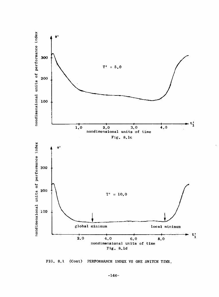
00o 200 \
r-
0< 300
1.0 2,0 3.0 4.0
'.4
c,4
200
Cd
rom 200
v4
En
0 t11.0 2.0 3.0 4.0
nondimensional units of time
Fig. 8.ld
F
CU
;. 30004
0
w 2004J I \ T' 10.0CU
o 100
global minimum local minimum
2.0 4.0 6.0 8.0nondimensional units of time
Fig. 8.1d
FIG. 8.1 (Cont) PERFORMANCE INDEX VS ONE SWITCH TIME.
-146-

II tl I
I II
oF
c
/C
CC
0o o
40
o 0
(o
0X
epu~ eouum-To~-Tad ~
o
s~
,Tu
n
ieU
OT
SU
z.
pu o
C'
v X
CudI
Io
-14
7-

00
/ a)
E
1\
.
N~m
T~
~~~~osTn
uo
Go
CD
omui
jo
sT
un
leuois
uem
ipuou
-148-

D. STEADY STATE SOLUTION
For a very long test, we can approximate the repetitive bang-bang
inputs with a sine wave. The system and sensitivity equations consist
of three second-order systems of the form
1l = -C 1X 1 - c 2 x2 + u
(8.18)
x 2 = X1 -x 2
where xl - x2 replaces u for the first set of sensitivity equations
and xl replaces u for the second set of sensitivity equations. The
transfer functions are given by
x (s)
uTW =
x2 (s)
u(s) =
s_+ 1
2s + s(c
1+ 1) + c
1+ c
1
2s + s(c + 1) + c
1+ c
2
A block diagram for the calculation of f
input is approximated by u = 4/i sin Ot,
is shown in Fig. 8.4. If the
then for a long test
8 2 M)2x (T1) = - TtM4( + 1)
8 TM4 w2( + 1)x8(T') = 82 2 2
x (T) 8= T' cos e M4W(w + 1)
where M and are defined by
where M and 0 are defined by
-149-
(8.20)

3
+ 4 v3I/ ..
4Cq
3 4-
3
+
^
3 +
3
CQ
3
C3
3 '-
3
II II
II
x-) ;
H
3
-4 cq ~ ~
h
+3 ce
3 S
O3 m
3
+
-4
II
w
.,1
+3 4
IIX
N
N
-15
0-

1
[(C 1 - )+ (C1 + 1)
(8.21)
sin 2 i+
(W + 1)
Substituting (8.20) into (8.12) and simplifying, we have
22= 8·22 2(8.22)
8 T'M4 w2(w + 1)(1 - cos i)2
Substituting for M(w) and e we then have
2( 2 2)2 + w2c1
+2 1)2
2I2(22 + 1)[(cl + c2 - )+ 2 (c + 1)
,,-~~ 1='. 1~~ . ~(8.23)
8T'w (w + 1)
For cl + c2
= 3.185 and cl + 1 = 3.15, this has a minimum of 'mi =
398/T' for w = 1.05. This corresponds to a switch time interval of 2.99
time units or 4.05 seconds. This is in agreement with the solution curve,
Fig. 8.3.
E. SIMULATION
A simulation was run using Denery's combined algorithm to identify
P1 = M/Iy and P2 = Mq/Iy from measurements of the pitch rate q. The
computer program for the simulation is shown in Appendix B.
Recall from Table 8.1 that
P1 + P2 = k 3 2
(8.24)
P1 ' k5 4 + ml = k34
so that if we can estimate k32 and k34 we can estimate P1 and P2 accord-
ing to
-151-

A 34 - m1P =
k54
(8.25)
2 kk32 P12 - 32 - Il
To use Denery's [DE-] combined algorithm, it is necessary to trans-
form to a canonical form where the unknowns are coefficients of the meas-
ured state q. The equations of motion take the following form:
(2) f:21 (x2 X2 (°o)/= 0 (8.26)
q = [1 o [] (8.27)
where xl = q and
= (f 1 1
x2 = k1 q + k2ce so that
+ k1)q + k2Y + g
1 18e
k2 = 21 k1(f11 kl) q - kla + k (g21 - klgll)Se
By matching the coefficients in equations 8.28 with the first two equa-
tions in set(8.8) we have
gll = 8g3 1 (known)
k2
= k3 4
f11 = k32 - k 1 = k32 + k54 (8.29)
k1 = -k5 4 (known)
-152-
(8.28)
f21 = k2 + kl ' k32 = k34 54 32 (8.29)
21 = kl . gll -k54 . 8g3 1 (known) cont.
If we can identify fll and f21 from Denery's algorithm, then we can
calculate k32 and k4 from32 34
32 - 11 k54(8.30)
k34 = 2 f21 +
k54 k32
Notice that we cannot identify all six stability derivatives (M& /Iy,
Mq/Iy, z /mu, Zbe/muo, Ma/Iy M5e/Iy) from the five coefficients
(k32, k3 4 89g31 , k5
489g
5 1) and with a scalar measurement we cannot
identify the above five coefficients from the four canonical coefficients
(fil f21' gll, g2 1 ). Since we are only trying to identify two stabilityderivatives, the scalar measurement is satisfactory.
For simulation purposes we use values for the stability derivatives
calculated from the five coefficients identified in Denery's 17-second test.
However, one other stability derivative such as M- Iy is needed or we may
make an assumption such as M. = M . The numerical values for this simu-
lation were shown in Table 8.1.
Now applying Denery's algorithm to the second-order system (8.26), we
have
fll 1
Fn = H
n= [1 0] (8.31)
where F and H are given byn n
-153-

F =n
H =n
F - DH
(I - L)H
so that for this example
L=0, *G=0, = 0 =, 0 D, =
Estimates of fll and f21 are given by
nf11 = f11 11
fA2 = n
21 = f21 21+ D '
The simulated measurement z, is given by z = xl + v where
X1 = fllxl + X2 + gll ' X1() = o
x2 = f2 1xl + g2 1 e 2 (0) =
The nominal output is given by zn= Xnl where
(nl\ 11 Xnl + Xn2 + gll x =e
\ Xn2! 21Xnl + ' Xn 2
The sensitivity equations for Dll and D21 are given by
1f 1 + 11 + z (or zn)
(6n2 = n PXnl'n
-154-
(8.32)
(8.33)
(8.33)
(8.34)
(8.35)
(8.36)
(8.37)
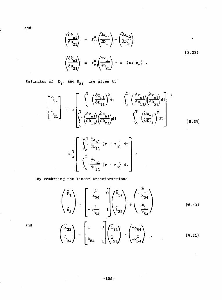
fn f )n
n /xnli2=2 +z
/Xn2
(8.38)
(or zn)
Estimates of
D
D_2 1_
Dll and D21 are given by
= r
ST (3x 2dt
T
0
( n1A
ii/\ ~21/
11 ( 21/
5T nx )
1aD__I)2 dt
Xr
- T
So n) dtaxnl
E ( z - z11
50 ED~2 (z - Zn) dt
By combining the linear transformations
1
1 lk54
1P2 k54
'54m
+ m1
1 k32.m ·k 54;
k3 1 0f1 1 k54\
3~~~~~~ 2 ,' ~F ~ ~ · -
k34 k54 f 234 54 1 21 ~~~- 54/
-155-
and ( nl21/
(I n21
\aD2 1
-1
(8.39)
and
(8.40)
(8.41)
T

we find that
A L51 /
k54 21
The covariance in our estimates of the parameters P1 and P2 is given in
terms of the covariance of fll and f21 by
Tp = E(p- t)(p- p) ) (8.43)
-2 1PDll +-p +pDll 'k54 PD12 2 D22
k54k54 k 54
1 1
k54 D12 2 D22
Pk54
2 PD22k54
For a four-second test, T' = -k54- 4 - 3.00. From Fig. 8.3, we
see that for T' = 3, N = I is optimal with t{ = 2.04 and V' = 228.
In this case the normalized covariance for Dll and D21 (or fll and f21 )
is
150
-80(8.44)
The predicted covariance for D11 and D21 is then11 21
5-Rk54
PD = 2 P
g31 ' emax
297 -159i= R
L-159 156
-156-
+ (8.42)
(8.45)
80
78

Substituting values in (8.45) with R = a A2t = (0.1) (0.01) = 10
into (8.43), the predicted covariance matrix for P1 and P2 is
0.0297 -0.0159
L:0.0159 0.0156
In the simulation, Denery's algorithm was applied to 20 sets of data
and the results are summarized in Table 8.2. Except as noted in the first
column, all of the tests had a bang-bang input with a switch at 2.72
sec, a standard deviation in measurements of 0.1 rad/sec, and an initial
guess of P1 and P2 of -0.60 and -0.80 respectively. The average number
of iterations for the 20 tests is shown for the equation error and the
output error portions of Denery's algorithm in columns 2 and 3. The re-
sultant covariance of the estimates is shown in columns 4 through 6.
From Table 8.2 we can make the following conclusions: (1) With an
optimal input, Denery's algorithm converges faster and to a more accurate
estimate than with a non-optimal input. (2) The predicted covariance
given by the inverse of the information matrix is very close to that cal-
culated in the simulation. (3) For large errors in the initial estimates
of the unknown parameters, the equation error portion takes more itera-
tions to converge; but, the number of output error iterations remains the
same. (4) An indication of the final accuracy in our estimates is pro-
vided by the number of iterations needed for the output error portion
of the algorithm to converge. In a sense, then, the bias from the equa-
tion error portion serves a useful purpose.
A computer listing of this simulation is shown in Appendix B.
-157-

N-14o~co.4)00co-,4$4. C
a
(U0C).
to
C
--
CD
0 a3
e 0
Vt
t0
to
0
0 0
0 0
0
o j
0J
0 0
Co
o-4
CI) -
I I
I I
a *
* a
a a
a a
to IfLOI
ooI)
0 0tq
ooo
(D
In
X
Hr
tDCD
LO) CC
,-I C
D
d C
t C
D
CD
cq t-
N
Ci
CQ
0 0
0 0
0O
(r
O
0001
.~
.1
.1
a a
a a
a
0
o 4~)
· 0
N
q t·
11 '
i
~ h
k m
r, c0 N
N
1
0C 0
I
4
0 o
'F
0
.,-I M
MH
L
t LO
0
OI
4-0
4-3
.X
t,
O
O
03
$4 co
0
II
O,
4 4
r .,
-N
.
U
C
Z
o
E
II II
*,- 4 11
4.) -
-15
8-
c/- o3I0 E-0E-
c:z-4n
i)
Icd
UbO
O
I I 0
coU)
.. bi
4. 4
CI
s @
=
c
0 H
0 P
C
a 0
0 )
II
@
00
PA H
O
QIC
(4 0
11 u
U]
_h ,
qq U]
Ooo
Ir@
wr
W
·r Y
O
IiI
.I

Chapter IX
OPTIMAL INPUTS FOR THE IDENTIFICATION OF THE LATERAL
DYNAMIC STABILITY DERIVATIVES
A. PROBLEM FORMULATION
Approximate lateral
plane are*
equations of motion for a conventional air-
B + r
Ixz
r + I Pzz
I* xz p+ r
Ixx
n¢Izz
Ixx
YV mV ~?+V
nr+ + I r
zz
r
I xx
n+
Izz
+ PIxx
nb r
p+ -- rI rzz
aP + -a 6
I axx
= p
- r
where
P = sideslip angle
r = yaw angular velocity
p = roll angular velocity
The equations and numerical values used for these computations weretaken from Bryson and Ho [BRY-1, p. 173].
-159-
(9.1)
*
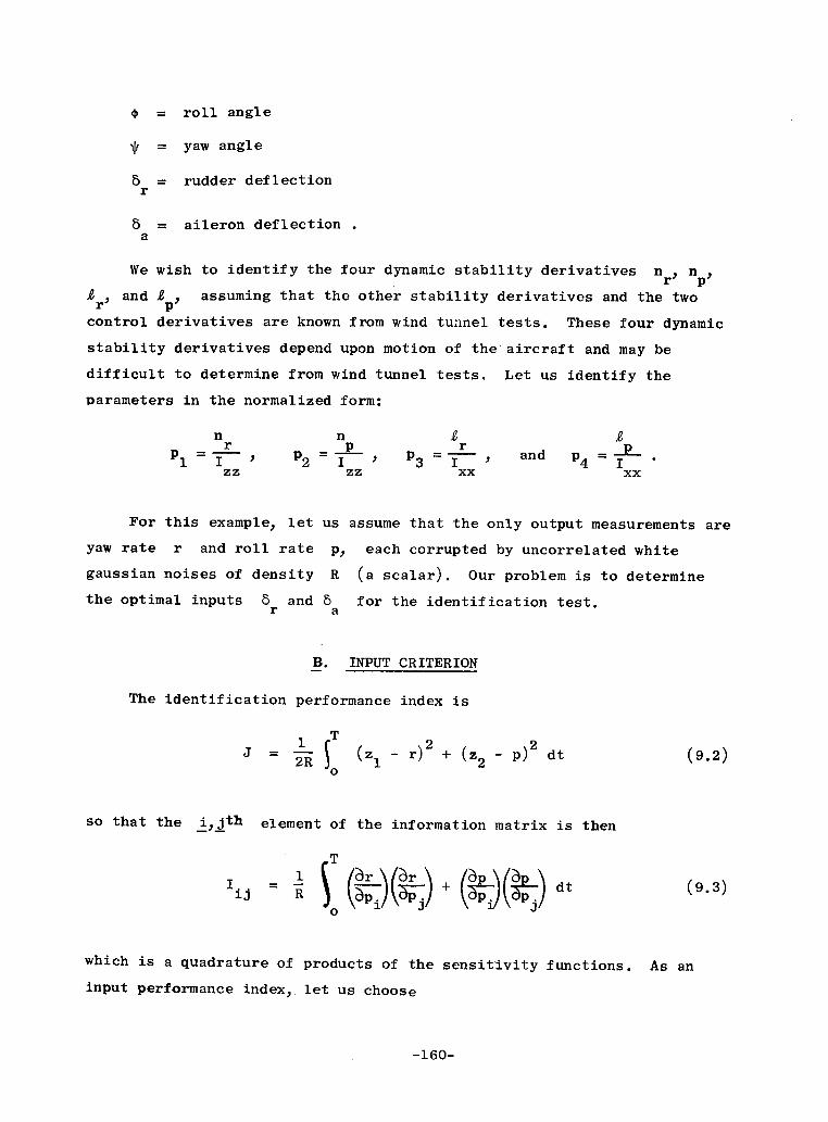
0 = roll angle
* = yaw angle
a =r
8 =a
rudder deflection
aileron deflection .
We wish to identify the four dynamic stability derivatives nr n p
Xr, and Ip, assuming that the other stability derivatives and the twocontrol derivatives are known from wind tunnel tests. These four dynamic
stability derivatives depend upon motion of the aircraft and may be
difficult to determine from wind tunnel tests. Let us identify the
parameters in the normalized form:
nr
P1I =zz9zz
n
P2 I zz
rP3 = I
xxand p I
4 Ixxxx
For this example, let
yaw rate r and roll rate
gaussian noises of density
the optimal inputs 8 andr
us assume that the only output measurements are
p, each corrupted by uncorrelated white
R (a scalar). Our problem is to determine
5 for the identification test.a
B. INPUT CRITERION
The identification performance index is
1 T J = 2R I (Z1 - r)
2
+ (z2
- p)2 dt (9.2)
so that the i,jth element of the information matrix is then
I. 1J
T
I (r rr\ r p(9.3)
which is a quadrature of products of the sensitivity functions. As an
input performance index, let us choose
-160-

= Tr I-1a
The four sets of sensitivity equations for pi,
are the same as (9.1) except that the inputs are
0
r
O
O
0
O0
P
0
0
O
O
r
0]
and
pO
o
O
o_
instead of
(9.4)
P2k P3
0
Izz r
l a0
0O
and p4
and the "states" are the sensitivity functions
ar
1
ap7p
a1
ap 'and '
Pi
where i = 1, 2, 3) 4. The last equation in each set), and 6*/6pil
i = 1, 2, 3, 4 is uncoupled from the other equations and may be dropped
since there is no state constraint on i and we are not using measurements
of ,. The system equations may also be written in the form
= c 13 - r+ c2O
r = c3r cp+ + c4r + c5P + c6 r 7 a
= c8 + c9r + 10OP + C115r + Ci25a
= p
where
-161-
(9.5)

C1 - mV
_g
2 V
IxzIz DXXXX ZZ;
C 8 =D
I I I
D C =9
n I nr Ixz r
ZZ zz xx
D
p Ixz IP
I I IZZ ZZ XX
D
nb r
6 I Dzz
Ixz 85a
I Izz xx
D
10
2C I n s
I I I Ixx xx zz
D
( I n_ xz pxx xxI Izz
D
Ixz _n r
I Ixx zz
C11 =D
Q5a
c12 - I Dxx
I Ixz xz
D = 1 - II I
The sensitivity equations for p1) p2, p3 , and p4 are of the same form
as (9.5) with the following modifications:
n8(1) For p1 substitute r for - 5 and set 8 = 0.
zz
(2) For p2 substitute p for - 8 and set = 0.zz
nga(3) For p3 substitute r for 85 and set 5 = O.
xx
(4) For p4 substitute p for - 5 and set 8 = .xx
-162-
c3
c4 =
c5 =5
C7
(9.6)

Evaluating the performance index requires 30 integrations (4 state
equations, 16 sensitivity equations, and 10 information matrix quad-
ratures) over the interval from O to T.
C. GRADIENT OF THE PERFORMANCE INDEX
The partial derivative of the performance index with respect to the
kth switch time t k is given by
=Nt- -TrI Ia (9.7)k ka (
The elements of aIa/6tk are found by integrating product terms involv-
ing xi and axi/atk, i = 1, 2, ... 20. The differential equations for
axi/ tk, i = 1, 2, ... 20 are the same as those for xi, i = 1, 2,
20, except for the elimination of the inputs 8 and 8 . They are in-r a
tegrated forward in time from tk
to T with initial conditions given by
ax.
C) t (t k if x il (9.8)F ~(tk) = xit -- xi (~k t=t t=t+
Evaluating the partial derivative of the performance index with respect to
the kth switch time requires 50 integrations (20 state and sensitivity
equations, 20 equations with respect to tk, and 10 quadratures for the
elements of aI a/tk) over the interval from tk
to T .
With more than one input, the assignment of switch times for each
individual input becomes a little more complicated. For this problem
the first input 8, has N1 switches at times tll t 2 t1,N1
and the second input 8 has N2 switches at times t 2 1 ' t 2'
t2,N2 . There are a total of N switches at tl, t2' ... tN where
N = N1 + N2. Figure 9.1 shows a possible switch assignment for the case
N1 = 2, and N2 = 3. Since the individual switch times are incremented by
different amounts, this assignment can change with each iteration.
-163-

5r
I I I
t1,0 It1, t tf
t t t It t
to tt l t2t tt t f
IIG. 9,1 POSSIiB SIC I AIGMNt ~ ~ ~ ~ I.91PS2.0IL SWITC TIMt I. t 32.f
l I I I
FIG. 9.1 POSSIBLE SWITCH TIME ASSIGNMENTS
-164-

D. RESULTS
The conjugate gradient search routine for the optimal switch times
is similar to the Chapter VIII Example implemented in Appendix A.
To insure a global minimum, we proceed as before by plotting the
optimal performance index for a number of cases that depend upon the
number of switches. For the scalar input case, we had one case for N
switches. With two inputs, however, we have 2(N+l) possible cases
for N switches.
For N = O (no switches) we have two cases: N1 = O0 N2 = O:(no
switches for either input), and the two inputs either start (1) with the
same sign, or (2) with opposite signs (i.e., in-phase or out-of-phase,
P =+ 1).
For N = 1, we have the four cases: (1) =1, N2
= O, P = +1
(one switch for input 6r, two inputs initially same sign); (2) N1
= 1,
N2
= O, P = -1 (one switch for input 5r, two inputs initially the opposite
sign); (3) N1 = O0 N2 = 1, P = (one switch for input 5a two inputs
initially the same sign); (4) N 1 = O N2
= 1) P = -1 (one switch for
input 5 , two inputs different signs).
Each of these cases is an optimization problem with respect to one
parameter. Figure 9.2a to 9.2d show the performance index 4 versus the
parameter of interest for a test length of five seconds. The end values
of the performance index correspond to an N = O case. The performance
index versus the length of the test for an optimal input is shown in Fig.
9.3 for each of the six cases of N = O and N = 1. Each case is specified
by the triplet (N1, N2, P).
For N = 2 there are six possible cases, namely: o (2, 0, 1),
· (2, O, -1), (1, 1, 1), * (ly l,-1), (O, 2, 1), · (0, 2, -1).
Each of these cases involves an optimization problem with respect to
two parameters. Values of the performance index are shown on a grid of the
two parameters of interest in Figs. 9.4a to 9.4f for a five second test.
Except for the (1, 1, -1) case of Fig. 9.4d, each of these cases has its
minimum at a minimum of an N = 1 case.
-165-
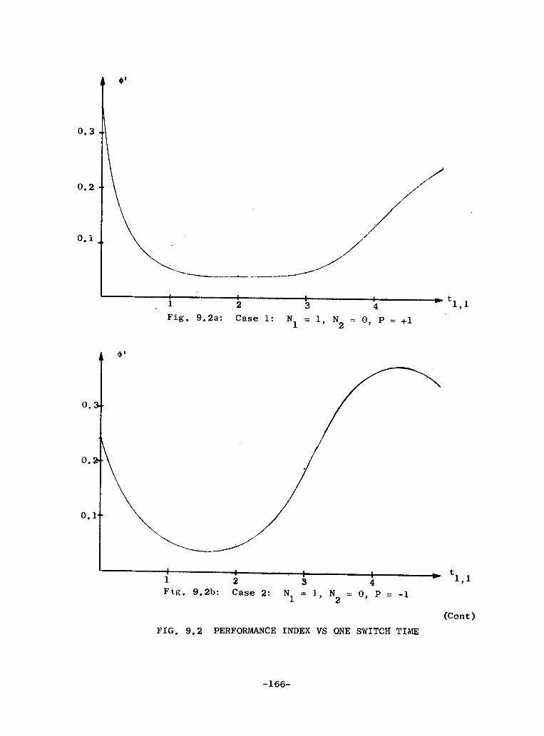
0.3 A
0.2
/0.1
I I I I ; t11 2 3 4 ,1
Fig. 9.2a: Case 1: N 1, N 0, P = +11 =1N 2
0.
0.
0.1
1 2 3 4 'Fig. 9.2b: Case 2: N1 = 1, N2 = 0, P = -1
(Cont)
FIG. 9.2 PERFORMANCE INDEX VS ONE SWITCH TIME
-166-

0.
0.
Fig. 9.2c: Case 3: N1 = 0, N2
= 1, P = +1
0.
0.'
0.
1 2 3 4
Fig, 9.2d: Case 4: N1 = 0, N2 = 1, P = -11 2 ' -
FIG. 9.2 (Cont) PERFORMANCE INDEX VS ONE SWITCH TIME
-167-
t2,1
t2,1

Solution shown for
-4 1R = 104 1sec
18aI S m = 0.1 rad
Keel 9 m = 0.1 rad
where 0 Rc 2m
(1, 1, -1) QI, o'
. .(0,'.0, 1)- (0, 0, -1)
(O- (0, 11)
- (0, 1, -1)
'-(1, 0, 1)
L, O, -1)
(2, 0, 1) - e
· · I , · I
3 4 5 6 7 8 9
sec
FIG. 9.3 PERFORMANCE INDEX VS LENGTH OF TEST
10
-168-
10.
1.0
1 -2
sec
0. 1
0.01
0.00:
1 2
l1
I
I I I Tr

N
O
N
Oq
,+ O
C
Doco
to co
c0
O
0 0
U
p
O
O4
N
0 0
0
OC
O
O
O
C
)
LO
tD
Ce 4)
N
I Co
r-
**
* 0
o 0
0 0
0 .
D
d' n
qq N
_I
O~~~~~~~~~~~~~a
-169-
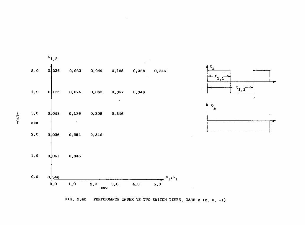
c eq d
0·
CD
v 0-
qD
oo LO
pq
' O
X
' D
¢X
~
m
ce c
t
Co
;o 0
c q o
CD t.
O0
)-)
Co
o0
~~
~
C
o o
o C
;
to
I- CD
'- 4C
Q
" O
t CX
0
w
o o
to
Co
-170-
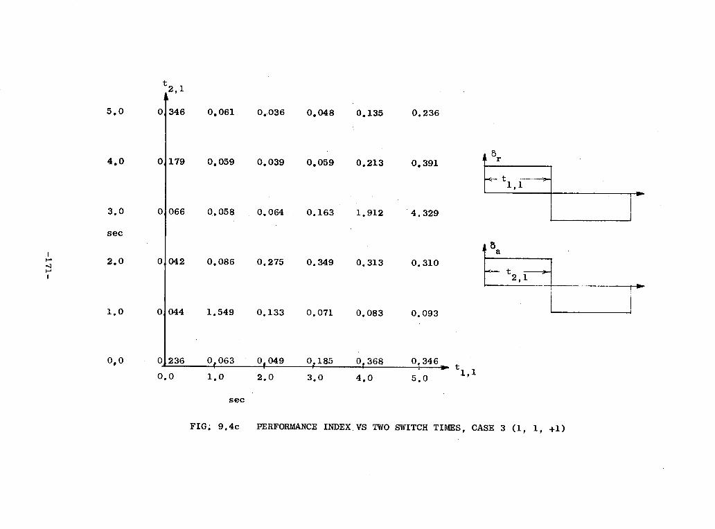
cJ,-
N
m,
m~~~c
(D
-I O
C')
CD 1C
r) ce
0V
cr) 0
C*
o C
o
C.
o o
o o
o0 0
I EC',)
CV4 v-4
i-I cc
CD
-¢ 01
0)
c') o 0
vO
Cto 0
, 0
0 0l '.
x L
w
ce
O
4o m
C
' U
) AD
U
r o
o )
C)
ce0) tD
C
O)
0o o
0 O
0
0 0
0 0
0 0c(
O
O
O
O
_e O
O
-.
vD
CD
CY)
4-I ad
CD
n o
-171-

CD
CD
0O.OO t-ooOcUOIf)oo.-4C
D
0
-4 CD
_-4 0
C0 0)
qC.4
_ .4
0
CY)
oCoO0
0-,oCOr
O
O
o
o
000o O
*
O
bc0-40~ cr;C
o
0, COOO-4
-172-
-4-44-)A
CD
coC.40V
CD
00
lo,-40cCD
O0O
VD-1
cph 0IrO
Ot
r-I
000CY)
c;,)CD
oCD-4CD
Co
C)
U)
'-4
0~oo C; ~
OnC0
cq
D0o,-4CD
o01 -4
O0If)
OO
c;Lr
0O0'
0C
4-- ,i

CD
O,
cq oo CD
0to0
CD
0,Iooo
Q
O0,
02 0,
CD
cqC
CD
o_
0,
B~
~~
~~
~e
oOI
o o
o
-17
3-
cO
o-)'a)
-I
o
j. If
-4
I-4EC
ra0
tDCO
c;00CV
-o0O
Q
0;
0-I
oc,), 4-I
q .
o
c,o4
o0ocM1-I00
o'-I
I)1.I
V:.
O
-

*TI -ccUI
rC.,(
CD
,,0~ C
O~
0
~:
CD
(O~
~ ~ ~ ~O
CO
O
o o
0
tD
XtD
C
o
o 0
0 0
tD,
CD It
lo o
0 0
to
t0
C
0 0
* *
..
.)
4 In
e c-
0a
a o
o
O
O
O
Q
oO
-17
4-
All six cases for N = 2 were examined in a similar fashion for
test lengths of one and ten sec. For the one sec test, each case had
its minimum at an N = 1 case. For the ten sec test, each case had
its minimum at an N = 1 case except for the (2, 0, 1) case. (The
switch times for this case were 1.5 sec and 5.3 sec for the rudder, and
no switching of the aileron.)
No N = 3 cases were investigated.
Unfortunately, these solutions cause such large deviations in the
state that the linearity assumptions are violated. One method of
satisfying the linearity requirement is the addition of state inequality
constraints. For this problem this means two second-order state in-
equality constraints on 1 and O .
With state inequality constraints, the steady state (assuming a
stable system) wave shape may be somewhat irregular. A Fourier analysis
may then be tried by optimizing with respect to the relative amplitude
of higher order terms in addition to the frequency.
However, these problems are left for future research.
-175-

Chapter X
CONCLUSIONS AND RECOMMENDATIONS FOR FURTHER RESEARCH
A. CONCLUSIONS
Optimal input design for system identification has been investigated.
The primary conclusions are:
1. The information matrix, I, (for the parameters of a linear
dynamic system) provides a useful measure for input design.
The criterion used in this thesis was the trace of I
(which is a lower bound of the covariance of the parameters).
Minimizing this criterion appears to have some advantages over
maximizing the trace of I. In simulations where the trace-1 -1
of I was minimized, I was a good lower bound in the
sense that it was approximately equal to the actual covariance
of the parameters.
2. An optimal input for system identification excites the system
as much as possible. With amplitude constraints on the input,
an optimal input is either full on in one direction, or full
on in the opposite direction (bang-bang inputs). The addition
of state inequality constraints can be important in practical
problems where the instrumentation and the dynamics of the
system must be maintained within their linear region. With
the addition of state inequality constraints, the optimal input
is still bang-bang but with intermediate values while on a
state constraint.
3. For long tests, the optimal switch times are often equally
spaced. In such cases, we may assume a square wave input and
optimize the performance index with respect to the fundamental
-176-

frequency using a few terms of the Fourier series for a square
wave. With state inequality constraints, the shape of the
input pulses may require several terms in a Fourier series for
an adequate approximation.
4. The results of a simple example indicate that for reasonable
amounts of deterministic input, the overall effect of process
noise is to decrease the identification accuracy. However,
for systems with no (or very small) deterministic inputs,
process noise contributes to the identification accuracy by
providing excitation.
5. The solutions in this thesis for the optimal aircraft flight
test may be modified to insure that the instrumentation and
dynamics of the aircraft stay within their linear regions.
One method of meeting the linearity requirement is to lower
the input amplitude constraint. A design allowing full in-
puts but with switching to meet state-inequality constraints
should prove better but has not been solved.
B. RECOMMENDATIONS
The following areas are recommendations for further research.
1. The methodology developed in this thesis should be extended to
include the addition of state inequality constraints. Of immed-
iate interest would be the addition of state inequality con-
straints to the aircraft identification problem.
2. The information matrix also provides a criterion for determin-
ing the best instrumentation to use. Instead of heavily instru-
menting an aircraft or other system, it may be possible to
obtain almost as much information with far less instrumentation.
This would not only lower instrumentation costs but lower the
complexity and execution time of identification algorithms.
Identification algorithms could also be structured to process
-177-

only those measurements that contain the most information (at
least for initial iterations). However, optimizing the best
input/instrumentation combination together would be quite
difficult.
3. As mentioned in Chapter III, more research would be useful in
determining the best model numbers (numbers that specify struc-
tural information about the system such as order or degree of
the minimal annihilation polynomial) for multi-input multi-output
systems. Considerations should answer the following two ques-
tions: (a) What is the minimum number of parameters needed to
designate an arbitrary member of the class defined by the model
numbers? (b) As the order of the system increases, how many
different cases must be examined?
4. The calculated value of the information matrix may vary with
changes in the estimated value of the parameters. Instead of
expanding the identification performance index to second order
(as in Eq. 6.1), we could expand it to third or higher order.
The third order tensor
E3J
)a3
may be viewed as the sensitivity of I with respect to the-1
parameters. In addition to minimizing Tr I , some measure
of this term should be minimized.
-178-

APPENDIX A
This Appendix is a computer listing of the gradient algorithm
developed in Chapter VII, which is applied to the optimal input problem
in Chapter VIII. A flow diagram of the conjugate gradient algorithm
is shown in Fig. 7.1, and a flow diagram of the one dimensional search
portion of the algorithm is shown in Fig. 7.2. Subroutine POINT cal-
culates the value of the performance index by integrating the state,
sensitivity, and elements of the information matrix, whose differential
equations are in subroutine FCT. Subroutine GRAD calculates the
partial derivatives of the performance index with respect to the switch
times, which requires integrating the equations in subroutine FCTP.
Subroutine ADAMS (not shown) was the numerical integration package used.
-179-

C TiE OPI IMUM INPUT TO I')ENTIFY Z PARAMETLRSC (M ALPHA DOT AND M U) IOF 1Hr' SHORT PERIOD DYNAMICSC OF AN AIRPLANE IS A BANG-OANG, INPUTC hITH SWITCH lIMES ULIVN bY lItIS PKUGRAM.C TUL FINI) THE GLOBAL MINIMUM CF JPt RUN THIS PF.C;GRAMC SEVERAL -TIMS wllTIT I)IFF'F4FNT VALUES FOR N AND PLCTC 1li. RESULTS. ACCURALY 1S C.MoIROLLED BY SPECIrF IGC I tAXAMI NLSMHINC JP = TRACE GF THE COVARIANCE OF THE TWO PARAMETERSC =NUMbER UF SnIlCiH TI:4[ INTEkVALSC T=L=LENGTH CF TESTC (l)l I = I TH SWIl(.H T I.MEC IthAX=14AXIMUM NUMBEk OF 11EHATIUNSC AMIJ=MINIMUUI INCRE.Mi-NT TG ASSIGN 10 ShilCH TIMESC SMIN=/:INlMUi SUM OF SQUARES OF PJ'SC PJ=PARTIAL DER OF JP wITH RESPECT TO SWITCH TIVESC LL=ZETA=DAMPIN(, kATIOC hN=UNDAFPED NATERAL FREQUENCY
REAL JPtJSJO,JI Je.J3EXTERNAL AnAMSDIMENISION O(LOItPJ(l, tX(ElSl, i) H(10,lOT eR(lC)t
L DR( IOi G(IG)t OLD )( )PJOLD( lU),DXI L)COMM]ON CI ,CZUCUMMGN/S1/NX, VltV2 ,V3,DET
I FORMAT('1',35Xt'ZETA=',F6.3,' O.-MEGA N=',Fb.3,C ' C1=:'F6b.3' C2= ',F6.3)
2 FORMAT(//' ',6OA,'N=',l4/7X,'T',TLX,'JJPP,9XC 'D(2) THHU D(NF1)')
3 FURMAT(I ',19.3,F13.5,1OF I.1.5)luO FURMAT(I0lQZFI'. 5I101 ;ORMAT (2F 1u.5J102 FURMAT(I13)
READ(5, 1)) IMAX, A} IN,SMINREALI (5101) ZE ,vNREAD(5, 192) NI,N2 ,N3,LLL2 L3C l =2.* ZE: 'WN- 1 .C2=WN WiWN-C 1WRITE(bl) LE, tu,Ci,lL2
UDO 33 N=NItN2,N3TN=NWAITE (b,2) N00)O 32 L=LI,L2,L3T=LOD 1)=O.OI)O 5 I=Z,N
5 U(I)=D(I -1)+T/TNDN+1 )=T[=0.2*IN-I )*1 /1NICNT=0
CCALL PUINI(JO)1F IN.EQ.1) Gu lu 3JCALL GRAU(IJ)
-180-

6o Lt.NTINUEICNT= ICNT+IK=lAOA=J.OOU 8 I=2tN
l.J 8 J=2tNt( I,J I=0.0
8 IF(I.EQ,.J) H(I,J)=I.OIf (ICNT.GF.IMAX) GO TO 30
9 CUNT INUEAI=ATDO 10 1=2,N
10 JULD(I)=D(l)RS=0.0PJO=O.ODU 12 I=2,Nit(1 }=0.090 II J=2,Z\j
11 R( I )=R( I) *H( I, J)*PJ lRS=RS+AS(R( I I )
12 PJO.=PJO+R( I)*PJ I )PJ0=-PJ/ RS
CC ONE DIMENSIGNAL SEARCHC
DU 13 I=2,N13 D(I)=U(I)-RKI)*A1/RS
CALL POINT{(JL)IF (JI.LE.)J)+.83333333'PJiO*A1) GO TO 15AZ=-. 5 PJ O:"A IAI / ( J 1-JO-PI'J*A 1 )U)EC=-. 5*PJO*AZDO 14 I=2,N
14 D(I)=D(I)-R(l)(1A2-AI)/RSCALL POINT(J2)I-(A.i ((Ju;-JJ-tDEC)/DEC).GE.O.1) CGO TO 17GU 10 20
l5 AZ=3.0*A1l)O 16 I=2,04
16 DII)=D(I)-R(I')*(A2-ALI/)RSCALL POINT(J2!
17 E i= (J -JU-PJO04A1 ) / ( Al*AlI)E2= ( JZ-J0-PJO0'A2) / (AZA2 E4= (E i-EZ )/ (Al-AZ EJ=Si-E4*AlIF (E3*E3-3.04PJO*E4 .LT. J.0) GO TO 20A>= (-E 3 eS ;RIF' { E 3;'E A-3. O:P JU*EE } ) / ( '.'O 9E4 )IF (A3.LE.O.O) Gll Tr( 20IF (A3.GE.6.O*Ii ,A3=6.0*AIIL) I 8 I= 2 ,N
18 J( l)=D() I-R,( ) (A3 -A2 ) /RSCALL PClIN (J3)If (J3.LE.J2) GO TO 22
-181-

00 19 1=29Nl 0(1)I=D(I)-R(l)*(A2-A3)/RS
CALL POINT(J2)20 AOP=A2
JO=J2GO TO 23
22 CONTINUEAOP=A3JO=J3
23 CONTINUECC ENrD OF ONE OIMENSIONAL SEARICHC
IF (K.EQ.I .AND. A(II.LE.AMrIN) Go) r0 3000 24 I=2,N
24 PJOL0( )=PJ(I)CALL GRAD(PJ)S=O.000 25 1=2,N
25 S=S+PJ(l)*PJ(I)IF(S.LE.SMIN) GO TO 30IF(AIO)PGE .3.O*AI.AND. ICNT .E. L.AND.K.EQ.l) GO TO 9K=K+IAOA=AOA+0.2*AOP/ N-I)IF (K.GE.N) Ar=AOAIF (K.GE.N) GO TO 6
CC CALCULATE H MATRIX
U0 26 1=29NDX I) =D:I1 )-OOLLOI )
t), 0)I i)=PJ(I I-PJOLDI)D00 27 I=2,1F1DR(I )=O.O00 27 J=2,N
27 DR(I =DR(I)+H( I,J )*0(JJD)ML=O.OOM2=0.0I)U 28 I=2,NDmt=OMl+4OX( I ) !J;( I )
28 D2=-DM2+DGI I)I)R(1 )DO 29 1=2 ,N00 29 J=2,N
29i H(I,J)=H( I,J)+DX(I )*DX(J)//DJMI-DR(I )*i)R(J)/DMZ2C
GO TO 930 CONT I NIJE
IN=N+ 1WRITE (6,3) T,JOD(I),I=2, IN)
32 CONTINUE33 CONTINUE
RETURNEND
-182-

SUBROUTINE POINT(JP)C VALJES OF X AT THE S.ilTCl T:4ES AND VALUE OF JP
EXTEKNAL FCTREAL JPJIMENSIJN DLO)J tXIL),X 15,11)XlS) ,AF( 1CO)MMIlN CI ,C2,COM.ION/SI/N,D,X,Vi, V2 ,V3,DErNN=9D00 1 K=LNNX(K, =O.O
1 XIlK)=O.ODO 3 =1 ,NU=(-L1)**( 1+1)CALL AODAMS.(NiJ+( I ) ,J(I+1) ,XI ,XFFCT)DO 2 J=1,NNXl I(J)=XFCJ)
Z X(JI+1)=XF(Ji3 CONTINUE
Vi=X 7,N+I)V2=X( 8 + 1)V3=X( 9,N+1)liT=V l*V2-V3*V 3PI'=Vl/CETi'1Z=-V3/DE P22=V/D)ETJP=PL l+P22RETURNEND
-183-

SUBROUTINE GRAD(PJJC PARTIAL DERIVATIi-$ OF X WITH RESPECT TO: SWITCH llFCS
EXTERNAL FCTPUIMENSION OlIJ),Xl l5,L),PJI 1)OXI( 15,XF(15)COMMUN CLIC2,UUOMMUN/SI/NUtX,VV2,V3,tlET
NN=15dJ 5 J=2,N
U=(-I )**(J+1)DO I K=1,6
1 Xl(K)=X(KtJ)XI (7)=-2.*UDO 2 K=8,15
2 XI(K )=O.OI l=N-J +100 4 [=1,11CALL ADAMS(NN+LDL I+J-1)0tD(+J) ,XIXFFCTP)Il 3 K=1,NN
3 XI(K)=XF(K)U=-U
4 (.UNTINUEPVI=XI( 3 )PV2=X 114)PV3=XI( 15)PJd(J)=-PV1*( VZo* z+V3*V3)-i'V2*(VL*V1.+V3*V3)
L +Z.*PV3*V3*(VL+VZ) )/UET**25 CONTINUE
RETUKNEND
-184-

SUBRUUTINE FCT (r,X,)x)C UIFFERENTIAL EQUATIONS FOR STATE,SENSITIVITYC EQUATIONS AND INFORIMATIlON MATRIX
DIMENSION X(15),DX(15)CCMMUN CL,C2,UI!Xl 1) =-ClX(L I1-C2~X 1 2)*UI)DX2)=X(l)-X(2)nX(3)=-Cl:x[3)-C2*X( 14)Xl)-X(Z
APPENDIX B
This Appendix consists of two parts. The first part is a computer
listing of the simulation algorithm developed in Chapter VIII. The
simulation consists of applying Denery's combined algorithm to repeated
sets of simulated data and calculating the covariance of the resulting
estimates. The second part is a listing from the simulation prdgram
for the optimal input case for a set of 20 tests. Of special note are
the last three columns which (when multiplied by R = 10 ) show values
of I based upon the estimated values of the parameters. These valuesa
ranged from slightly under the true covariance (shown in the last line)
to 50% over the true covariance, and indicate the sensitivity of the
information matrix with respect to errors in the estimates of the param-
eters.
-186-

C IDENTIFICATION SIMULATICN USING THE OPTIMUM INPUTC TO IDENTIFY M/ADOT AND M/q FROM THE SHORT PERIODC DYNAMICS OF AN AIRPLANE
REAL K32,K34,KN32,KN34,K54,Ml,Kl ,K2l,KRII,C KR21,K14
DIMENSIGN U(luUO),Y(OOOXI( 50),XF( 50)1,C ZL(OOOO),Sw(1O),ST 6,.100) ,SUM(O1)COMMON U,Y,SWTtFL,FL ,F2FNII,FN21,Gll,G21,Z,
L K14iK54, GKll,K34,SWNNEXTERNAL FCT1,FCT2
I FURMAT(8F10.5)2 FKRMAT(313, iX,10O,2FIC.5)3 FORMATi'1',30X,' IDENTIFICATION ALGORITHM',
C ' WITH OPTIMAL INPUTS'/' N=',[3,' NT=',13,C ' IP=',13,' IX=',I10,' S=',FIO.5,' ACC=',FlO.5)
4 FORMAT(' SWITCH TIMES ARE ',10FlI.5)5 FORMATI' K54='tFl0.5,' Gll=',FlO.5,' Gz1=',
C F10.5,' Ml=',FlO.5,'KII=',FIO.5,' K14=',FIO.5C /' SIMULATED (ACTUAL) VALUES OF THE UNKNOWN ',C ' CONSTANTS ARE ON TFE FIRST LINE'/' NOMINAL ',·C 'STARTING VALUES ARE ON THE SECOND LINE'/C ' VALUES USING DENERY"S ALGORITHM ARE ON SUBCSEQUENT LINES')
6 FORMAT(//40X,' TEST NUMBER',13/2'PK22' ,7X, 'P11' ,88XX, 'P12' ,8X, 'P22')
7 FORMAT(' ',14,2(2FLO.6,3F11.6))8 FORMAT(//' K-STATISTICS CALCULATED FROM THE ABCVE 'i,13,' TESTS'/9X,'FII',7X,'F2L',7X,'PK21',7X,'PK22',27X,'PL',8X,''P2',BX,'P X , ' 2',8X,'P22)
9 FORMAT(5X,t2(2F10.6,3F.11.6))17 FORMAIl' ',I4,ZFlO.6,33X,2Fl3.6)
C INITIALIZATIONAM=O.ODO 30 1=1,10
30 SUM(I)=O.0DO 10 i=1,50
10 Xl(I)=O.OC READ IN FULLOWING PARAMETERSC N= NUMBER OF SwITCH TIMES +1C NT= NUMBER OF TESTSC IP= PRINT OPTIONC IX= RANDOM NUMBERC S= STADOARC DEV OF MEASUREMENTSC ACC=REQUIRED ACCURACY OF 10 ALGORITHMC T= LENGTH OF TESTC SW= SWITCH TIMES
READ (5,2) N,NT,IP,IX,S,ACCWRITE(6,3) N,NT, IP,IX,S,ACCREAD(5,1) (SW(I,I=1l,N)WRITE(6,4) (SW(I),i=L,N)T=SW(N)NN=N-1
C KNkjwN COiISTANTS FOR TilF C-8 AIRPLANEG=3 2. 1KEAD (5,1) K54p,GL,MI,Kll,K14GZI=-K4S Gll
-187-

kRITE(6,5) K54t11,G21 tML,KlI,K14C SIMULATED VALUES FUR UNKNOWN CONSTANTS
READ (5,1) PL,P2K32=PL+PZK34=P1lK54 +M1Fll=K32+K54F21=K34-K54*K32
C NUMINAL VALUES FOR UNKNOWN CONSTANTSREAD (5,1) PSI,PS2
C A CALL TO ADAMS WITH SUBROlJOINLt FCTIC GENERATES TRUE INPUT AND OUTPUT
CALL ADAMS(5,0.0tT ,AI XF,FCTr I Pt, C ALGORITHM REPEATED ON NT SETS OF DATA
DO 21 K=1,NTICNT=OWRITE(6,6) KWRITE(6,17) ICNTtFIIF21,PIP2PN1=PSIPN2=PS2KN32=PNI+PN2KN34=PN1*K54+MlFN1 I=KN32+K54FN21=KN34-K54*KN32WRITE(6,17) ICNT,FNtFN 21,N PN1,PN2
C NUIIMAL RANDOM NUMBER ADDED TO MEASUREMENTDO 11 1=1,401A=O.O00 50 J=1,12IY=IX*65539IF(IY) 55,56,56
55 [Y=IY+2147483647+156 YFL=IY
YFL=YFL*. 4656613E-9IX=IY
50 A=A+YFLV= (A-6.0)*S+AM
1I1 LI)=Y(I)+VC IUENTIFICATION ALGORITHM
SWT=1 .O15 ICNT=ICNT+l
IF (ICNT.GE.10) GO ro 20C A CALL TO ADAMS WITfi FCT2 GENERATES NOMINAL OUTPUT,C SENSITIVITY EQUAlIONS ANl) NECESSARY QUADRATURES
CALL ADAMS11,0.0,T ,XI ,XFFCT2tO,1)W1=XF(7)W2=XF(8)V1=XF(9)V=XF (10)V3=XF (LIDET=V *VZ-V3*V3PK11=VI/DETPK12=-V3/CETPK22=V2/DETKRI 1= ( V 4Wi-V 3*2 2) /DE TKRZ1= (-V3*0l1+VZ*W2)/DETFN 1=FNL+KRI 1
-188-

FN2 1=FN21+KR2 LKN32=FNLI-K54KN34=FNZL+K54*KN32PNL=(KN34-M1)/K54PN2=KN32-PNIP1,=PK 1+2.*PK12/K54+PK22/K54**2P12=-PK12/K54-PK22/K54**2PZ2=PK22/K54**2WRITE(6,7) ICNT,FN1I ,FN2 1,PK11,PK12tPK22,PN1,PN2,
CP11,P12,P22C If CHANGES IN ESTIMATES ARE LESS THAN ACC THEN PROCEEDC TO STEP 2 OR IF ON STEP 2 STOP
IF (ABS(KR11).LT.ACC .AND.ABS(KR21).LT.ACC) GO TO 16GO TO 15
16 IF (SWT.LT.O.O) GO TO 20ICNT=OSwT=-l1OGO TO 15
20 CONTINUEC SIORE ESTIMATES FOR LATER ANALYSIS
ST(1,,K=FNLLST(2,K)=FN21ST(3,K)=PNIST(4,K)=PN2SUM(I)=SUM(1)+FNL1SUM(2)=SUM(2 ) +FN2SUM(6)=SUM(6)+PN1SUM(7)=SUM(7)+PN2
21 CONTINUEC CALCULATE THE ACTUAL MEAN AND COVARIANCE
SUM( )=SUM(1 )/NTSUM(2)=SuP(2)/NTSUM[6)=SUM(6)/NTSUM(7)=SUM(7)/NTIF(NF.EQ.1) GO TO 23WRITE(6t8) NTDO 22 J=1,NTSUM(3)=SUM(3)(SSUM(L) -ST(L/,J))**2SUM(4)=SUM(4)+ISUM( )-ST(,J))*(SUM(2)-ST(2,J) )SUM(5)=SUM(5J+(SUA(2)-ST(2,J))**2SUM(d)=SUM(8)+(SUiMib)-ST(3,J))**2SUM(9)=SUM(9) (SUM(6b)-ST( JJ))*(SUM(7)-ST4,J) )SUM(LU-J=SUM(1IOU)+(UM(7)-ST(4,J))**2
22 CONTINUESUM(3 )=SUM(3 )/MNT-.I)SUM(4 )=SUM(4 )/(NT-1I)SUM(5 )=SubM5 )/(NT-1.)SUM(d )=SUM(8 )/(NT-L.)SUM(9 )=SUM(9 )/INT-1.)SUM(1O)=SUM{LU)/(NT-1.)jWRTE(6,9) (SUM(I ) ,(==I10)
23 CUNT INUERETURNEND
-189-

SUBROJUTINE FCT(Il,X,DX)C GENERATES SIMULATED INPUT AND OUTPUT MEASUREMENTS
REAL K32tK34,KN32, KI34,K54 ,,tK ,K21,KRL , KR2 ,K14DIMENSION X( 5O),DX( 50),U(IO0O),Y(ILOOO),Z(LOC),SW(IO)COMMON UY,SwT ,FlI,F2.1,FNIiFN21,GLtGZ1,Z,C KL4,K54,G-tKl K34, SWtNNI-INT(LUU.OI*T) +1Ut()!=0.2DO 10 J=INN,2
10 IF(T.GE.Sh(J).AND.r.LT.SW(J+1). UIl)=-O.2UX( I=Fll*X(1)+X(2)+GII*U(I)[X(2)=F21*XA1) +G21*U(I)DX(3)=XCI)DXL4)=KII*XC4)-G*X(3)+K14*(K54*X(I)+X(2))/K34Y( I )=X(1)RETURNEND
SUBROUTINE FCT2(1',X,DX)C GENERA[ES NCMINAL OUTPUT AND SENSITIVITY EQUATIOKS.C PERFORMS QUADKATURES.
REAL K.32,K34 KN32, KN34 K54 ,MIK ,K21 KR t KR2 1,K14DIMENSION Xi 5U),DX( 50),U(1000OYIOO)), Z(IOOC),SWI10)COMMUN U,YSwT,FIL ,F21,FNLlFNZl,GltG2t1Z,C K14,K54,G,KI I K34, SNN
I=INT(Ioo.0I*T) +1DX() =FNi*X(l )L*X ( 2) +Gll*UI)DX(2)=FN21*X(t) +G21*U([)YD=X I)IF (SWT.GT.U.O) YD=Z(I)DX(3)=FNll*X(3 )+X(14 ) +.Y)OX(4)}=FNZIX(3)DX 5)=FNII*X(5)+X(6) DX(6)=FN21*X(5 )+YDX(7)=X(3)*(Z(I)-X(1))DX(B)=X(5)*(i(I)-X([))CX(9) =X( )*X( 5UA(1U )=X(3)*X(3)OX(IL)= X(3)*X(')
E TURNLND
-190-

0.
7 I NenOJ
J 00
7d 0z
-ne
.aa4
,<
_-
Vr
7 -
.-4
tO
N-
0
0
C$0 . 4
S _
a ,,,
tu
0 )
0.)
N
Nt
-4
L
NC
) -
.J ).
J _ Z
Z
U. 0
-" Z
.O
l- .. .'
,N
1
I u
a. U4 J
4
IZ
Z0
aD
O
*30
_O
10040
N
U.
J
IN
6 )...
0 0
4 .
-4 J
I O
N 4
VO) .o
0 U'
NO
* I 0
U-..
T0:U
NU
zW
O~
L
Iwt
:r: r
>
V y
n Z
0 O
co
_' 4t
a0 N
0co a
: -
N 0
' 0e
en 1
N
000)0N0N
O.4 en en en
C
_ _4._
N
D N
L0
0P
N'0
.0 N
10
e n
0N
en. O
0
0 a
en000n00
1 e000
-4-
_- N
N
N
N
N
C en
0 0 0. 4N
_ e.
e
.-- N
e
cr,
-o0000.NW)
_ OD
0
0 cm.
00
en e
enm 0
o4
000
e 000-
0 0.0)
Ln
0)1
t1
co
co 00
O
N
N
N
N
Nc. 001
e m
0
e;
.4.
* .
..
00000000
00
O Nen ' e n N
C 0.
.0 o. C
:e C
YC
OZ
4 4 4
N
N
I I
cu 0·~u
)1)(.
0.
0 O
-40'
'ON en
N
r n en
0 Nr e
o. N
P4
00.40.010n_
! no^
_ en 4
aK *
4 4
4 -4
en N N N
-4
U-4~ t
-4.4
-4-4
-41 N
in ..
0 0) 10
a- 0Z
~
fr n
IDC
en N- CC 0
0 .0 eN
N_4
N .0 10 0
N~ j.
Ir U
'
U. N
4 N
U)
N
N
N ,
0N
* ...
....
o. 0
N 01
en 0.4O S
e..-
.w en Nen e
_4 N
fs
N 0)
et y0 0
0)
U _U
. en U
-41114
1010
..
..
4.
.4
N
N
N
N
N
N
N
N
S 00O._
N
en ¢
NtUN
LA
0 0
-
-
0
enO aur 0
N 0 I
in
-gN
N
U
00 G
Go
0 0 N
Nen
en 1t 0-
N
-00
.0 0
. 0. 0
0
0. 0
N
m
0a Go
00
_ 0
LA
C)
M U
.*
-.
..
.0 tU
U
U .0
000
' N
N
-4
0 0
N
tr 0 00
N00 N
N 0
4 0-4
N
N
4
4
N 0'
O
N
N
N-
_l-
0000000
00 O
U04.0 N
0
4O
a a
4
40
N
__
40
N
CD G
o
-_N
N
IIIIooII
4 en 4
_ 0
0 G
o 44
N N
U
N
° CI It
Va
.W
. .
Oa 00 00
U N
I00
N
.U
4
-N
O0
O
a
* .
* -.
_N
P- -N
* o
O
1 0U
f
LL M
.010.in04
-0 0
-4 -4
-4
00
N 00
N 0
0.0
. 0 cu
N
N
V 00O
_ N
._
N
4-
4 40
am
c,
4 n
0
-¢t
4 t n0
N
'C 0
_ 0
0'
NN
'0
.O
'-N
0)0
.0O
N'0
_N
m
CD .4
rj0.
..
4 .
0 0)
N
0 0
u 10n0 O
t r-
r 0
.00 0
N
o O.
e
Om
OnO
1010
C N
_ a
-N
N
Nt n
.. e n .n
n
OO' U
'%O
'N
Oen N 0
v 90
-410 C
C
-4N
a -
* * .
.
N 1 0 10 0 0
0.4410
10r-
40 e
U N
0 U
o N n
co
n N
N
.
£6o ,
866
co 3 (-
O
O
en eN _
c 0.0
* a0.
.*
o 4C
o
4 -
,4
04 0
0-4
-4
-4
-4
-N
* ..n -
.en
.
, 1en t
nr
czn
N
N
Lo
ON
N
mC
-0
01
4 4-4
VCa
* *
.4
a .
0n0 00 .70
0)
1000.C
.N
- C
, _t
UN 1O4
en .
Cy 0
-41 0
OY
0
CO
_
00 N
0. ¢ .0 N
.40'
O
)'
C en
en
Nf N 10 N 01n
-4
in.0 co
C
4 '
4 It
I '
4 C
II 400IIr
en N
z Irz C N
Z
10
.N CN
N
M100
.0
N en en ¢
0
00
t0 cO
-19
1-

uN
0F o r
0En 1-
-t
-e -M
4
Eni 4 En
0
U' O
ct _
f
N
1-O
-M0
.U
tv 't tr% IV
I
l1
co
4
aFn r
IL
* .
-.
n M
N
N
N
0
.4
.0 0
q:U
NC
0 C
N4
N
4 .0
N '
N
_ .t-
N
) 01
_ ar
0. ffi .
..
.
n0
E
a4 C
y
_y M
n
enMC) r
o .4
-el
'D0
N a,
't 0.'
0fi. .0.0
*'
0 -4
N
-N
0.
.- .
.ar
' cd
.4
Nr
NN
En
En n E,
0 0
N
'O
o cc a
0 I0
N0
4n 0
t00
N
o N
00O
4oe~ N En En1-a
fi b
b >
oL
.' -'.0 .0.0 .
'
0000000
gI
es
I
004.0
4
~.0
o4
o
@
o 0 000
o0 0.
a 0. 0
' _0.
0..
.14.0 a.0
. 0
0000000, c
I .
I
0a NN
Ul
zI.-%A N_.4
L
-0fn
40 .
O0 _ 04
N
..UN c
r4
N -
N
0 ..
* .
4*-
E 0
'e .4
e
0 '0
0
En
O
0 04 01
N
4 UN
aO
c_e
Os
o ev, O
_. 0
n O
~ 0-
O E
n 0 En
En1- N
00~
0.4
q4 N'0
1O N
N
U.
E
-N
N
N
N
N
N
a,' 0c
4 0
n
nN
0
0 P.
0. .
-
4 4
-0 N
-0
En
N
_.4 'a
1d- V0
N
N
N
M
0
MO
- N
N
00't4 0.
1- F-
0. *
* *
4O-
O
(C
N' C
t N
.r-
C D
t- O
u
-4
-4
-4-
4
_ _
^ _
_ __
tn C
) N
0
.4 C
-.
n NN
7 '
en
a,
~ rn 0'
1,- LA
I-
e 0o
.N
0
4.t)
N
CO N _ 4
4
n
-4 M
o co4
N M.
0 0O' .4
D
-
04
0'
0 0
1-
0.0.*a, M
' 0a'-
, *
.ll, O
it .
Al
44
0C
t
o 4
'OM
n4
a"- .
-
-4
e'-Enaoo a,4
N
) 0 co
LI
-P
- I
'00.0o 4 o
_E
n
000n
-0
a,
a , 0
0 0
4 0.0.
00.~~~10 0fl.0En'
_ 0
0' C'
'0 .
C"
0C
O
n C
; 4 4
4 000000000OLQ
00n.
En a,
04
a,
~00 En 0.0
441
-
0 0 ,'
' 1'-
-4
-t 4-
(y rer
K
<1~
O.4
O'0
.0.0
.0.0
' 0.
O'
0. O
1- 4'
0.
Oa '
.O
.' O
.4
..
* .
..
000000000
S
l 6
@
116I
eL 0 0
' O
' 9 O
' tT' 0
O'
0~
0000000
I |
| (
|
O NN
$0.
U!c.
z
a, .0.
N
En It
n I _
e.
4 0
N
'A
-4N
U
N
n
a 0-
.N
M.011
N
10 0
JSJJ4JJsCV0
~ 0~rr~~
C~
0
~~··SO
`JO
0
~r
4$Jn~nj~JQ
4 E
n'0
M0
i a, M
En r0o.V41.
EnOr-
0 Fr-
N
a_ C
'0
41
0 4
00.
Nr.
tr U
%
U\'
O.
0 E
n n
O-
EO
En 1- N
U- 1
au 1- -
N
fti 1-
1-1- N
N
NN
En 0. a
C (4'
0
O
O
0
..
* .
.*
.*
I1111111
_ rNn Et
t P
t -r- .-
N
N
N
N
NN
N
N
-OO- N
0 Ln.
N
U-
0O 1'
N
_4 C
D.0
N
.,C
.Y0
N 0.,
11
,,'4
U
04 I,- a)
N
t-1-a
n-4
e'.
N
E n O
O
N. O
C. *
..
.C
nt% O
Y
CD
- 0I"
-'0
4 '
'O 0
N0 N
a,"0
- '
ar -'0
4 a
0
N-,40' N
O
.
0 0.
_ O
1-
, _
_ C
0 CY ,
..
.4Z
00f .n .-.
0
-4
t ..
4 ,
c'4o
O'
EN 4 N O
eV
O4
N0
0. N
-M GO
y .o
-
aO
o I
4 _-
N
a 0,
01 ell 0
C ;
an 0
N 00
a
000 1
, -
IN
N
.4 0. 0
1- a
O a,
ao 0 0'
00000000
4 0G
' aE
0
C)
O O
- N
- 4_
0NON
'O M-
..
0N '
.4N
O
O
- N N
cO
_ O
C
O
f
4 0
�D o0
000000an
_ N
N
Cn
_0 O
N
-4 1
4
_ O
D) O
O
D
Y
1-m
D0
c0 N
4.)c00.
'4.4
0.-4
-0
-L Nr
En o w
w
o
w-E
EN '0
U
t. U--
IL 1-r-0 0..0
G0
* 44
*
.-
..
N-4'
a,
(E En En 1-. C
,LL
4 N N
N
Nm
N
N
N
N
N NN
N
N
N
L61111
I
oC0O
N~
tr
ee
ee
~~
0
4 Un NA
LA.
0.i .
... .C
.
*0
N
N
0 a'
~.01-1-01
1 t-
O
r-
U N
OM
en 0
VN 4
_ O A
-4
0.L
n
P-'
0. *
.*
4N
N
I
00.
011- t
ct-
-4-4
-4-4
-4
4-0 0 0
0 Enr- t-
En (.
-4
Mn o
M n' u
.*
* 4t
*
001- 0
N t-
0a
4O
Ca
4 .+
aO a
N
O N
0E
CY N
N
I r-0
00000
00.4
4N
OO
0%
L
En
4
00
0 .0
O
N
00 N 0
0%
n0
0C
C
0 44
0O
N
O- E Wnu
O0
v n'4
4 -0
.
uj
_cr%
P-
7 U
,4 0
M 0N
LA
- _ N
0
uVN
N
0 -
0N
.*
-.
.%
00000
11111
m004 O
IY
--
to CN%
P- C
. a,
1C- n
0C E
al N0I cO
0o C
M
O.'
N.'
0 O
C
O
E
C 0
* L
.
e .
.n
at a 0
N M .6
N
.N
C
44_____
*IIIIIII
-19
2-

N
O.0
4 't
r Oa
O
r-
IO
_ in
! !
-4 4n O-m
o
N 0'
j 0'in
0, r-
_00 ,
0
_ 0
Ir 00 a,
00
fl
00
.-
1
0 0
.'-
IO -
OO
0 00
-O
c ° °
u
o rr
r-N 0
r0
0- fei
m0eN 00
AP
r- 0
co-
P P
-P-
Al
a .
o en rr
M M
M
4 _
n. -
D 0-
co CC rD
fP r
4 I-4
I
OD
4N
r r-
r- O
M
-I r0
U
N
INN
U
A
N
'A 00
C
N
rn
r- C
0 G
0 rn
e0
IA r-
0M
I' -
-0
N
1-%A
N
mrrr
U
_.4
-V
N
w.
4y O
0'Ifl
N N
be
a *
.*
..
arN
00
0e0n en
O cr C)
a
aY
It C
t -
aS *
(. a .
N
A'F
O
' 0NS
004
4'4
-4
--4 -
4
UN r-
I- .4
N IU%
0M
t- N
4 40
.0_
N
' _
N N
O 0
X ^ fW
C
C
oC
C
,,
00'
r- 4
(I
0' IA
0000'
F.
.0 A
0
M.
Nr 0 N
N
N N
N
F0
-4 0
0 0
0
uN
N
N
N
N N
N0
0N
N
N
NN. N
U,I- P.n(
OL
(
-r-
w
r'- -
r- 0
N4 r-
0
q ro
N
O
r
'O4 ,4
-4 ,-
0'
_, 4 ,
o rIrt
r4(
o, o
,. n
.M.0
N
00
M- N
--N
M im
( ,( rt
,e
ON
04
Cyt
_0 tt
5'O
5'U
No ' N
NIA
2000
00,0
ar 0 IA
00
II I
n0
0 Is0r
,0' 0 N
%
NC
O
m
rnr
l In
J%
* .*
4
a O,
20 0
NM
4 4
n
OC 0c N
Nq _.
-r
00
00
4+C
. 0
4 .4
-c
-4
-4
000
000
a 00 -_
N
N
F A- UI
0rO
0 IA
-
O
'-40
I-
A-f
t
0 A
4 U
i Co
" O
.., cr
_iu
NC C
IA
a'-L
IN
-4
i.-n -4%.
_ IA
ts N "1
.
N
I U
N
P
- N
n
O'
N
O
CL S'O
i
Pr-
a .
* .
* *.
r- r-
00
o ar-
UI
.40
0 IA
UIA
-4
.4
-4-~
4-4
-.4
0 0
_ o) 0r-
IA
IA 00o5-
-4-4
UI
IA 0'
N
00000
.... 0
0M
40
IN_
co N*r rr
N.N
4
-P-0 _A
'
_r
_O
M
in
4''t
ct
.X
.
X
X
-4
4 4
-4
-M
r- r-
r 0
LA
muI
I I
U00 N 0i-4
4
O0
I- 4
O
M rg
CN "I
0 P- -
_ )
1 O
11
1
'
_ 0' 0
C
.D '
0 O
,4
0 i rfi
.D4
-C
s
r~ o _ N
N
t0
an
C; el nre
N
e000 00
00
.4
_O
' N
Ln
O4
O0 O
' -'O
00 O'
Ucm
O IA
'
M
_w
_ .N
40
4 N
N
N
0
' n.-
N
0'
0O IA
IA
8 1n
4 4
A.
A
0 I.
A-
t-. A-
I'-t*
..
....
co n
C O
, 0
, O
r O
D
CO
00000000
I ll
lul
lsl
0o
0rr.n
A
- r-
-0
0 .1 N
IA
IA
C
r 0's
4. 'O
4 4 M
4 C
O
_ (M
O
'- O
P4
U%
o 0Cv
* .
..
..
.
J -
O
Cc
C)
O
.nmU
. le
O
reb
DP
t
IA
0r_
0
IU
0 -
P.. IA
000
0
DlNr .A
...A..
N
..a
P-0
'.C0
N
0
~40 D
+
' 0f4v(
U-
C0
0 O
rr.
in
Yn
O
vrt tb
r-t
-n r0
'O~
OI
C r-.
co
0,
N.
I
M
* .M,
.M
*
O'4
04000
_ -
M
SO
4- 0 S
SL
L 0 0
O-
00
-I
5--0
0 r.-o
00
N0
4a
.-
* .
..
4 N
N
N
I- -I
r4 m U
t %
U
, V4'
4 .r
IA In
44
IA r.
00
N
00
rnA
'r0e
r'- '0
0
IA
It. re
Es
_N
000
00
-_-a
' ao
c nrn
O
C r
o
Uc c r-
O
0 -
r- r-0
'0
* .
.4
* .*
0'
0ws4
0 4.
P-
rr
0 0' N
O Cf-
-_ O
_ 4
U
0^
1trr
-44
.0
n o 0
0000
AL rr
.4
"
0rr 4
00
0
* .
* N
N
N
N
N
N
N
N
s t
u ese
r O
O
- N
O'.4
_N
U,1
1
5- -
4n
.[C[4
_ r
NN
_
.4
0 4
N
-4'0
U
''
N 0
h
c0 0)
0oN
0
U
4 4
I 4 I
a s
l
OD 4
I. 004
eN C
)O_
-CC
r- --
0 F
0
A
C
-
in
.4
..
N N
N
NC
-4O
a-
-4 -4
_ -
N
N
4 4a
-N
.0 N
N
N
0 O
Ny 0m
U, %in
A
IA IA
u s
r rco
in o g
s.
e .
* N
r4
0
I A
I
4 IA
0 0 4 N
4 N
N
40 0-4
N
-
Cy
_ t t
nfW
( U
L11_N
M (
N
0u O
I 0N
-_
F
'0UL
Ln
0 IA
O
C
C)
OA
Cy
000
N
f -
r-0
00
0
(T * -
a n .
'0
' N
N
N
0 4
CY
M
.C
O
'O
CO
U
0.
N
t- 0Co
N
oo.
0 40 0 -
IuA '0
O
0
IA
u
_o 0
.0
n C
D0 M
N
CO0'-4
o0 M
O
Y,0
4
o0
o I
r- en1-
N
04
f4 e4 4
'S 4
.*
D
.*
CD
-*
a *
..
..
.
M
C'
DM
0 GO
C
nj
fl 000000n
CP
aIica-ILC
_
0000.0
0
in N
0 0
0' a
-N
0 -4
0 -4
N
N
N
N
-_4
issa
bu
m
_d _w N
0
0e 'O
00 m
.0 0-4
N
r-
0'
0'
U'.
U)
CD
-4
O
* tt
IA4O
i 4 0
-t -A
0
10M N
N
0
I
N
0 0
0n ro N
lr-4
-4r- 4 -4
-4
-4
4 In
o- 0
4 4
r- F
-_
N
'0
00
0 0'r
A
tC
N
OP
t -r- P
- t- . 0.
U. A- A-
A- C
A' t'-
U'%
7 F
0''
0 P- N
0-
t-0
o,
0o c,.
r- 0-
00D
-4'
00
0 a'
0'
N 0
-4 N
0~
..-4O
00
N
NlL
0t
_ *'1
r'.. N
N
N
N
* ..
..
..
.N
N
N N
N
N N
N
00-N
O
4 ..N
uj
U,
I-~~
rlI~-
jC
.4
1)1
-193-
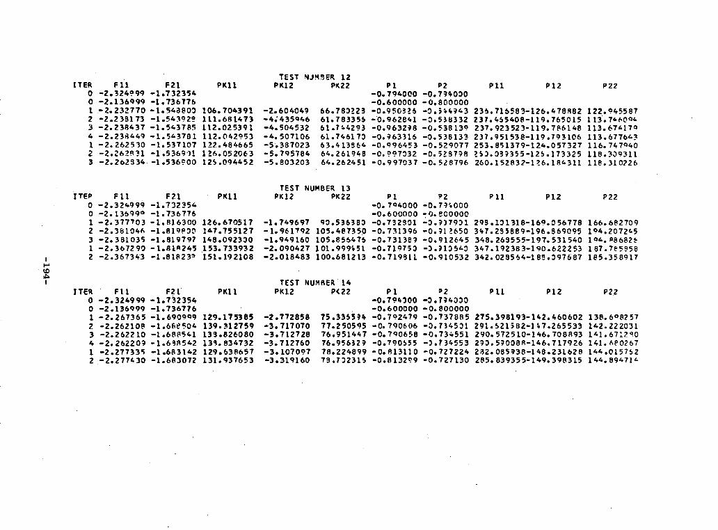
as 0
'0 0-
'.0
P
44 4
r s-
a o-O
M
~
Nen
c -
.O'
NA
t 4
P.
P.
00N
P
.4 -J
*O
-4N
0O
-P.0
.0
-e',in
a. ..-
O
-I.
.
No
rFl 0 0
0 a
N
-4
_ _4
__-4
-4-4
.4
.4 44
N
if. CD
.0-
UN _
0 _ -4
4
N
N
-
0 U
.0
en n
e 4N
F
ZF
o.
u(,s
=
0.i .
..
*f *
...0
0 O' O
' 4s .fl.S
0N
.4
-_._
N
N
1%
I" c
in a
. o
en N
Go LA
Ir uM
t- M
O
N.in
N
- cn
_ 0
0e o
. 0 0
_
0.
* .
*. *
* .
400
in
C
0
u%
U
" en
CD s
N
f N
N
N
,.. N
O 0
.(
N 0' r
tp
0'
.t 0
; O~
O
CO
00
N
0 o
.4 0 0
0 N
I.
N
.*
...
444....4
Oo O
%
D _
Ci r
^ t-
00
a0000
0 00
Oy a
t~
n ID
N ̂6 O
O00.0D
.0 0
A
f L4A
NAF-i
0j 0 4%
1 4
fr. .
e it, en0
0
m
O
N
Ifln 'O
00
4 00
NS M
M
. FO-
f.--4
0' 0
It. W
.0
.0
O
O
. e'
0a P
- 10'
O'
0'
O
O
O'
* 4*
4 *
* .*
000000000
| | |.
· 1
11
15
5155
on
h in
0
40
-4"
en e 5"-
.4e
4 e N
_i
01O
' N
N
N
Um.SN
I-
a.
004.0
0s-_
N
f
* *4
4 *
* *
-aD
_ _
_ 0
¢ k
co
44'O
N
00
o W
-4
0 I-N
I-
U
u e
-- t- n
in
en W
o U
U
.0
LU.*
*n
n
.4 to
No
mtO
o
enn
p.4 .e4
nU
in N
-4
O0
0N
4 0
4
O
-0
_ -N
I
N!
en
*D
O
C
.-
CO
' D- M
0 N
0 O
0in
.
C
0o 5.
-40
' CU.
N040444
000
* .
co
fr. .
-Ill
5 5 II
I I
i- -
NJ 0
C0 rN
N
N
N
NN
N
N
N
N
N
N
C 0
0- O
N
0w 4.
N
0L
WO
-
0' eV.
0I 5-4
e4 U
0
c, CD O
~
O
W,
GO
0t
N ¢,
C, O
N
P.
.0 It.
0N
0
n 0
CD L
N
.0 N
0P
. CL
0a.i
..
4 4
00 0
0 00
0e0
an f-
P.
e 4
en 0P
. 0
0 N
.0
U'% co
00 e-
_N
F-
N
eU
n.0
N
O'
_ O
L-A
IOa.
* *
.4
O'
.0P
0
a.C
0 0'
Un in
-4
0
en C
0 Uin
CD
t sD
en,_4
go en N
0
-an
C
O
0D c N
.4 .4
Aj
Y
40
_ N
en
_ 0
O C
-4
0 o
U
n N
O
0 0
44
W0
o 00.
r. en
en.4 0
p. .
N
o 0
N
ii 0
s- _
-4
_-_
..
* .
.*
.0000000
ooo Ce
CIl.
o c
on m
M
-
CD
**
..
4 *
O
0000000
co o
. h'P
_
CD e O
.,4 N
UN
0
N
'a.; *
..
.L
i O
c;
D
0 000
0
cm
PN
0
en' O
' 0 N
OD
leN 0'-'0
' J_
4'0
4
.4
e
y .
0 N
OD
_ N
060
~0- _
O'
en O
to N
-4
.4
CenN
ON
~
.4 i'n
A
j n C
Y
a.
..
@ .
.
.0 F
- 0
UN
-C
-C
-444-
.4
00
O-
O
-en
m
en p
en
0
' -4
0t P.
i- 0. W
N
N
.-, N0
0 ccc
0'
c 0
N
00
ma- .4
-
U. P.
P00
0
c4 M
M t-
JD
Z
1
..
.M
.
4 4
.4-4
.4-4
-44-4
)11,1
5m
g
0'0
'0400'e
4-
0 .4.0
O
- O
I <
_4 N
in
P.
.D 0.0
.0S
* .
..
4 .4
N
N
N
N
N
N
N
CL 00.4
N
0-_
N
w
~ r
S.-r-~
e-
n a (D
. _
N
o N
N
L
A'
0 N
4
u
n N
O
NF
IC
O
DN
.
N
.0*C
O
C
DC
. .
.S
.
..
C
N
_ -4
't 4
N 00 .0
0
n0
0e
N
N
-4
0 en CD
P- "D C
N
0sD O
-4
O'
-N
-0-
00eN
sal
I a
I N
0
CC
0 en
0 -4 N
0 fe
n 0
en
0 L
on
N
en
N
N
N
N
N
N
o0
c e n U
UN N
-a
O
0 t-
4t
4 Ft- N
-N
00 tn
00
'.i N
0000o000
000'
.00
en 00
40
N 0
00
00
.0
a-
a 01
0,
-1
O 0
00
00
00
lillils
-Na.C-
z
CL
V) N
I- lO
.
en 5A'- n. 0
. %
o e
enenNO
·tv
o,
Crul _
0 A
00 t O
.n
0 -4
QD
t N
q0nU'
Lt U
l.N n
LA ~r- Al
en
P N
e o'
N
P. -. 0
-
N 000F
0e
IllN
DO
0 0F
1-0
n ,
0 N --
Y
_A
s 0
e0
en e.4
r 4
.C4
O 5'-
.4 Pa,
.4 N
0 0
CL *
* 4
.*
40'h
e7
0.' 0
'-N
V
000
NO
4.0
0
-4Ch
w
N
N
N.
c-
O,
0IIW
4
5i
_. N
.0
0 80
C C
0 0 0
a- O
00'
400
00 f
U .
P. .0
. 0.
0. 04 .0
0' 0'
en O
_
O
e 0
IL e
_ N
N
0
4-4
4.0
P.
N
N
N
U' P
._
NO
. ...
5- P
.Z
D
U.
0.4_ N
N N
N
N N
.. 4
.*
4 .
* N
N
N
N
N
N
N
N
* i
I C
CZ I
I1
1.
S._
-19
4-

sr tt
t-
O '
_ ..
O
IAC N
N q'0
O
.e
N'C
o'
0a0'
O r-N "e
I,N
.
r N
0
.0
I.
-4 -4
e4
-4 -4
~6 * ,N%
..0C
4
en- fO-
C) t en
.tN
M
4t4 0in
o
*,-
-4
-4
-4
I I
II0l
d'
0 CD
0
o. tLD tf
en
,In
II _t
.0C
A 0
..40'
O
-t in
' °trt
00440.
0'.
pI in Ien
..
.t.
..
00
<
O
O .
W0
0
4.
r999
..
.9
..
.
.4oO
00
I I I
I I
I
00
OD 0
ID
U
0C) C
) .-
4
N F~ ue
o N
r U
q
co
.U
0
e~ N
OD N
U
0Me- ' 0. 0.0. 0.0.
c m 0 .
cm
IN
N.O
_4500l _
UN. M
* N
I e
a N
en
_
I- 0N4'1N
'
.0. .
4 .
S
-O
N
N N N
_4
n0
.u Or-IA
-N -
*n .aO
40
*._1
0....
4*
* 4044~
~-4
-4- r
r-4
-4-
ISS
S
S00 oI'o-?-0
0.0' --
'4IA
0' 0 1-1- .-
4-
4'C .IAIA
4N 0.
n e 10'0.
U. .-4N N N N
* .
S9N(N N N N N N Nl
5l15l1599a
04 .
U) lrc
r~I'-()
o 0.4
N 'C.'
en _
1' 4
-40.
en a.
0 n
IA
u00.4
N N
N
FN
1
.1
O O
.-
N
CN
e?44N
a
* *
* 4
o .4
000
C,'
4IA n
e'N% en Len
V% I7
0-o
In
en
en_ -O
O
-4
-0N4 co
co4 tWV -
,4
M
4 oIA 0
O~
M
en
M
O't*
N
'D
lS
UN I4
-4 -
I 'n
en
0N
4'
_-
r_ 0
O
0
C. *
.4
* *
0
II n e
n
It O
'C
Y
4-
-I IN
IN
in
_l
M
U,_
'III''
.O' .O
N N
N 1- 1-
000
In
4 0' en 0
_.- OD
t- t0
N
_~
U
+
^
w
0
_._
N
0
. 0.
N
0a.
..
.*
.
4% p ~C) -4
-4-41 0.
en
0 a'M
OD
O
'N
N
N
N
N
N'
0 00. "
400' 0
0'
001-0.f1-
-N. -4
o -4
en o.
en
en
IL
-4
r -
r-
In
n It
_U
.ol
0 o
IC
en
CO
cr frn
n
t 1
) an 1
* *
* ...
* .
000)n
000
00
N 0.0
en O
.
aO0
00
.CC
Y
n -
04
0
0 I- ID
1-
.O
'4
0 'C 0.
n' 0.1
*F
- O
co
4 t
c o00M
W000000
It O
D
n oV
rvJM
0.' U
O cO
C
Y
en
A N
'4 N
0 4
0
n* N
N
O
O'e
N
.0
ra
..
4 4
.CU
D
F0
00
00
E
Y._
I0
-I 0
-N
_ O
1111116
a *n a
en -a
ec.'o
D
In
U LA
40-4
_0.
N
0-4_
Nc
t c-0
a-4
1
_0 .
coN U
0 4' N
U1
0.
4 fy
a.i *
..
.4
4 60 e 4
.4 Nq
N~ N
f' 0.
I-4--4
-4
-4
'-4
M
4 f_ N
-0 eN
0.
N
0I
.0
C.
ni
-4* cm
'W
M Q:. a
h
M
U.
1-
r-.-
'- 1
- 1 1-
ell
44
--e
U
-4
-
0. C0.1- D. u's
040.e
0'
U 0-I
.-,
10 -
0 4
0.. .0
r'. 44
- 4 _4
-4 4'
1- N
N
N
00
CN .1 -O
Da
r)0.
a.U
. m-4 N
N
N
N
N
N
*.
... .
.S
.
N
N
N
N
N
N
N
N
cc 0 0 -
N
4 .4¢ N
ruh
5-
-4
'.- e.4 .x0
,0N4 -
I t
oN
.0
0t
t r
o '00.
%AC.
O .
c .*
f- O
D
N
N
0 _
0
_.
O,
4 00. 4
- _If
.I IAN N
IN
,D
-, 0
1
-4i
* .fi
.W
4
! N
N
-4
._4
.000r
-N
o0
0 D
n
co
rn
00
0.
o
O N
O
o N.^
00
I I I-
0 t -
0 0
en. 0
0 r.
e
000
C) 000
I II)II
1- c_N
,-I
t~1%
LV
I NA I
i N
I0 1N
0
0
0 M'00 N
in e
n 0
.4 IA
'
N
N
4 U
A0n U
IA 4
C)
UN 1-
.00.
* .
* .
0.0
00
0.-
4 -4-
t N 1- 0. N
e.
N 1O
0
IC'
e n _
Uen IA
n '
* .
.4
-4-4
-4-4
-4(
III'S
1
VI
0 *n
00 0o
M en0.
-4
NN
0 0
4 -4
-4
-4
a.4ri
en.c
r
.4
0.1-
N
en
aI. -4
_
_4 N'C
IE 1
I 4In
N 0.0.)
4 4 -
4 4
I r- 1-
0.CM 0
C- .
..
.C
*
M
M
0 0 N
4
M
.1)
0.
0 W
, o a 0
a 0
00
_ N
0.
n N
I-
-19
5-

o M- w
N
n 0
O
t. .-4
0'
_ N
.t
Ac) 4
4 4
-0
0 0
0D 0 0.
_ N
C
N
,.4
._4
N
4 U% Ln
4 0
Nco
4 4 t
tCo M
irg
n- _%
o. 4t
4 utf.
4 O
0
c, 0'
0.-.-D
_4 NO
_ o
4
<r
_ 0
. .
..
..
O N
0 f
t- t'
I'J e
DI- O
CO
tn
U0 .I
-4
0 --
4 0 -
'0
N
M0 tv
N
0'
I- I
I I0I I
I I
N Ns fN
N
' C
o 444
(LI 0 eM
00
N
Cy
N
N
Dv .
0 0
en
L.00'
O
_
I00
00
O
re
0a
4 0 P
O
0
U N W
. U
O0
a- en
UJ 0
a.
a- IC
,' a, a,
0 0'M
a,
...
.* *. .
gal
a
gIaI
_a- O)
0 cc, N
-40
.C
. N
N
0 ?C
O
f 1N
_ -
0' -
* -
a .
* .
, .
_ 44_ 4
n4 ee
-,
CO/ 0
0
f- 0n
U%
U'. 00. 9N
d 0'0
0
0 U
'. '"
in
,
N
4.0 4N'r
0 'N
CaC' N
O
_4 U
+
U
I uI IL I
fI
_ .0
0 U
U
en
N
r co
o 4 F
4 .n
0 t-
N
Nt -
tO
ON
-r- P
0.-
i-
-r
0C
00.t
I en
N
O
O
O
40
0?
00' a-il'
a
I a
a gamma,
el
-a- n
r- _M
N
N
U
*n n
NN~
0i.0
0
-0'0
.C
N ̂
O Ln, M
O
' 'o 0 f-
M
0c
.N
..
.4
W
M
.N
u o M
co
g*o -
*N
n0 U.
?--
0' 0 '-4
1-
4 0
0 0
0eI
en
' N
Nc
O
Z
N
+
g
0-4 A in in
0 O
OD I0
-U
nQi O
0
J N
-O
0°
aI *
.-
-*
-.
a *
-* *
In
44
CyNN
_N|M a l
a a a
g a l
a
0 ?-?
- M
P
- -
NAU
4 N
r-0
0'
_. O
NX
OO
NN
N
a
4 *
4
44
* *
M
en en n
N
.0?
P a-- 4-
re ? r-
0 ? -?
0
V4
-e n M
0
N
0 e
CyM
U.
Cy
4 4
0o o0
0
0' a-" 0'
N
O
N
N N
N
N
N
N
L% N
' 0
-N
en
.) N
en
I- N
~m
r I
.04
-4 _^ DN
_ N
en
00
_s '
.F
cr rc
cr
Cm
_ _sM
¢
U
o P
- -
r l
-
4 V
I
M
N
NA
O
4 or. c
_0'
en en
O'
n.
-N
) N
N
-4 -4
-4 -4
-4
en?- -en
en en
0_ * N
'
0 -
.-
.-'
.0
N
O 00
en en
N N
U.?
-?-O
a- a-a--?
,*
.4 *
.44
N' N
N
eN
4 N
N
-4.
0 0
0 ' 0
.1
' 4
N
N
N N
rN
N
N
u mama
ma~~
c ~ 0 0 -4 Nn en
.- N
·
a.-
a. _ca
N
a
0 Ct
N
I- O
n 0
tN 0 O0
N
4 O
_G
-
W. '.
- 't0
.4 t
-t. n4
N
40N 0mb_
.. U
.4 .
.0 N
¢N
0f-
tL O
' O
,
_
N I
I I
ID -
-4 -n
-4
O
OO
oO
N
W
OO
' O
n
N P- t-N
N
_ O
n mn
eO en N
-4 O
.Un
UN
'
O
-O
0
0
n
00
000
N
0000000
Sem |InalI
ON
N
N
U-.--C
L -49Lc
O
Nt n
0DN
' _ 4'M
0
.0 N
0 Cy-
en et
OD An.
eO
* .-40
.4
OD
AO
N0 CO
N 4
0 0
0 '?
O q-
M
-4 -4
-4
OW
U
o
^ ^
F
In
0 co
-4 u I
o?-
o
Y
N'0C co0 U
Na
l **
..
N N0 Z
0
Nen eM
en
-4_-4
4
n P
- N
0
0 0
0r?
- t-
L. .0
a. W
_N
0 4Iu
In N
N
N en
.0'
0' 0'
0' 0'
LL
*
-P r-**
P-
M 0'
N
D
0' a-'
0'
?
F-4 4
' N0N
0' N
N
N
z 0
-N
0
44
90
' 00
0' UL
en _
N
N
N
N
N*
4 .
* *
.-
I-.. N
SN
N
NN
N1
1 I
I
eC~cc O
~N
Nu1
-19
6-
U%
00a.
0N-4
N
-.0t.0
_ N
'-40,,1-
N-4
eL coI4'
00o IL0
o
UJ
0e, 0
·O
-.
P-
0
0'4
O
0
N 0O 0
u.0 ,.
_N
-
:) 0
U.4
4t
Il

REFERENCES
Aoki, M., and R.M. Staley, "On Input Signal Synthesis inParameter Identification," Automatica, vol. 6, pp. 431-440, 197C.
Astrtm, K.J., and P. Eykhoff, "System Identification - ASurvey," Automatica, vol. 7, pp. 123-162, 1971.
Barankin, E.W.,Stat., vol. 20,
"Locally Best Unbiased Estimates," Ann. Mathpp. 477-501, 1949.
Bhattacharyya, A., "On Some Analogues of the Amount of Inform-ation and Their Use in Statistical Estimation," Sankhya,vol. 8, pp. 1-14, 201-218, 315-328, 1946-48.
Breakwell, J.V, Stanford University, Stanford, California,personal communications, Spring 1972.
BRY-1 Bryson, A.E., and Y.C. Ho, Applied Optimal Control,Publishing Company, Waltham, Mass., 1969.
Blaisdell
Denery, D.G., "An Identification Algorithm Which is Insensi-tive to Initial Parameter Estimates," AIAA Paper 70-34,New York, N.Y., 1970.
DE-2 Denery, D.G., "Identification of System Parameters From Input-Output Data with Application to Air Vehicles," Ph.D. Disserta-tion, Dept. of Applied Mechanics, Stanford University, Stan-ford, Calif., 1971.
GI-1 Gilbert, E.G., "Controllability and Observability in Multi-variable Control Systems," SIAM J. Control, vol. 1, no. 2,pp. 128-151, 1963.
IC-1 Ichikawa and Tamura, "A New Method Based on Gradieht forSolving Optimization Problem with Bang-Bang Control," paper,1970.
JA-1 Jazwinski, A.H., Stochastic Processes and Filtering Theory,Academic Press, New York, 1970.
Kailath, T.,tion, Parts Ipp. 646-661,
"An Innovation Approach to Least Squares Estima-and II," IEEE Trans. on Automatic Control,Dec. 1968.
-197-
AO-1
AS-1
BA-1
BH-1
BR-1
DE-1
KA-1

REFERENCES (Cont)
KAL-1 Kalman, R.E., "Mathematical Description of Linear DynamicalSystems," SIAM J. Control, vol. 1, no. 2, pp. 152-192, 1963.
KAM-1 Kaminski, P.G., at Stanford University, 1971, personal com-munication.
KR-1 Kroy, W.H., Jr,, "Identification of Aircraft States and Param-eters," JACC preprint, pp. 302a-302b, 1971.
ME-1 Mehra, R.K., "On the Identification of Variances and AdaptiveKalman Filtering," IEEE Trans. on Automatic Control, pp. 175-184, Apr. 1970.
ME-2 Mehra, R.K., "Identification of Stochastic Linear DynamicSystems Using Kalman Filter Representation," AIAA J., vol. 9,no. 1, pp. 28-31, Jan. 1971.
ME-3 Mehra, R.K., "Optimal Inputs for Linear System Identification,"unpublished paper, 1971.
ME-4 Mehra, R.K., D.E. Stepner, and J.S. Tyler, "A GeneralizedMethod for the Identification of Aircraft Stability and ControlDerivatives from Flight Test Date," to be presented at the1972 JACC, August 16-18, 1972, Stanford University, Stanford,Calif.
ME-5 Mehra, R.K., of Systems Control, Inc., Palo Alto, Calif.,personal communication, 1972.
NA-1 Nahi, N.E., and D.E. Wallis, Jr., "Optimal Inputs for ParameterEstimation in Dynamic Systems with White Observation Noise,"JACC preprint, pp. 506-513, 1969.
PI-1 Pierre, D.A., Optimization Theory with Applications, JohnWiley & Sons, New York, 1969.
SA-1 Sage, A.P., and J.L. Melsa, Estimation Theory with Applicationsto Communications and Control, McGraw-Hill Book Company, NewYork, N.Y., 1971.
SA-2 Sage, A.P., and J.L. Melsa, System Identification, AcademicPress, New York, N.Y., 1971.
SI-1 Silverman, L.M., "Realization of Linear Dynamical Systems,"IEEE Trans. on Automatic Control, pp. 554-567, Dec. 1971.
-198-

REFERENCES (Cont)
SP-1 Spain, D.S., "Identification and Modelling of Discrete,Stochastic Linear Systems," Ph.D. Dissertation, Dept. ofElectrical Engineering, Stanford University, Stanford,Calif., 1971.
VA-1 Van Trees, H.L., Detection, Estimation, and Modulation Theory,John Wiley and Sons, Inc., New York, N.Y., Part I, 1968,Part II, 1971, Part III, 1971.
WO-1 Wonham, W.M., "Lecture Notes on Stochastic Control," BrownUniversity, Providence, Rhode Island, 1967.
WO-2 Wonham, W.M., "On the Separation Theorem of Stochastic Control,"SIAM J. Control, vol. 6, no. 2, 1968.
-199-