ohio’s learning standards mathematics

ALGEBRA 2 MATHEMATICS 3 COURSE STANDARDS | DRAFT 2018

1

Mathematics

Ohio’s Learning Standards Algebra 2 and Mathematics 3


2

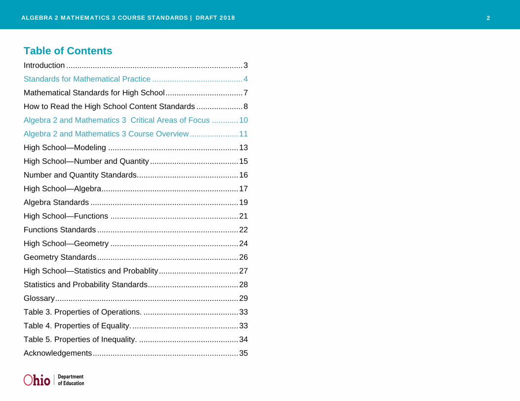
Table of Contents Introduction ................................................................................ 3

Standards for Mathematical Practice ......................................... 4

Mathematical Standards for High School ................................... 7

How to Read the High School Content Standards ..................... 8

Algebra 2 and Mathematics 3 Critical Areas of Focus ............ 10

Algebra 2 and Mathematics 3 Course Overview ...................... 11

High School—Modeling ........................................................... 13

High School—Number and Quantity ........................................ 15

Number and Quantity Standards .............................................. 16

High School—Algebra .............................................................. 17

Algebra Standards ................................................................... 19

High School—Functions .......................................................... 21

Functions Standards ................................................................ 22

High School—Geometry .......................................................... 24

Geometry Standards ................................................................ 26

High School—Statistics and Probablity .................................... 27

Statistics and Probability Standards ......................................... 28

Glossary ................................................................................... 29

Table 3. Properties of Operations. ........................................... 33

Table 4. Properties of Equality. ................................................ 33

Table 5. Properties of Inequality. ............................................. 34

Acknowledgements .................................................................. 35


3

Introduction PROCESS To better prepare students for college and careers, educators used public comments along with their professional expertise and experience to revise Ohio’s Learning Standards. In spring 2016, the public gave feedback on the standards through an online survey. Advisory committee members, representing various Ohio education associations, reviewed all survey feedback and identified needed changes to the standards. Then they sent their directives to working groups of educators who proposed the actual revisions to the standards. The Ohio Department of Education sent their revisions back out for public comment in July 2016. Once again, the Advisory Committee reviewed the public comments and directed the Working Group to make further revisions. Upon finishing their work, the department presented the revisions to the Senate and House education committees as well as the State Board of Education.

UNDERSTANDING MATHEMATICS These standards define what students should understand and be able to do in their study of mathematics. Asking a student to understand something means asking a teacher to assess whether the student has understood it. But what does mathematical understanding look like? One hallmark of mathematical understanding is the ability to justify, in a way appropriate to the student’s mathematical maturity, why a particular mathematical statement is true, or where a mathematical rule comes from. There is a world of difference between a student who can summon a mnemonic device to expand a product such as (a + b)(x + y) and a student who can explain where the mnemonic device comes from. The student who can explain the rule understands the mathematics at a much deeper level. Then the student may have a better chance to succeed at a less familiar task such as expanding (a + b + c)(x + y). Mathematical understanding and procedural skill

are equally important, and both are assessable using mathematical tasks of sufficient richness.

The standards are grade-specific. However, they do not define the intervention methods or materials necessary to support students who are well below or well above grade-level expectations. It is also beyond the scope of the standards to define the full range of supports appropriate for English language learners and for students with special needs. At the same time, all students must have the opportunity to learn and meet the same high standards if they are to access the knowledge and skills necessary in their post-school lives. Educators should read the standards allowing for the widest possible range of students to participate fully from the outset. They should provide appropriate accommodations to ensure maximum participation of students with special education needs. For example, schools should allow students with disabilities in reading to use Braille, screen reader technology or other assistive devices. Those with disabilities in writing should have scribes, computers, or speech-to-text technology. In a similar vein, educators should interpret the speaking and listening standards broadly to include sign language. No set of grade-specific standards can fully reflect the great variety in abilities, needs, learning rates, and achievement levels of students in any given classroom. However, the standards do provide clear signposts along the way to help all students achieve the goal of college and career readiness.

The standards begin on page 4 with eight Standards for Mathematical Practice.


4

Standards for Mathematical Practice The Standards for Mathematical Practice describe varieties of expertise that mathematics educators at all levels should seek to develop in their students. These practices rest on important “processes and proficiencies” with longstanding importance in mathematics education. The first of these are the NCTM process standards of problem solving, reasoning and proof, communication, representation, and connections. The second are the strands of mathematical proficiency specified in the National Research Council’s report Adding It Up: adaptive reasoning, strategic competence, conceptual understanding (comprehension of mathematical concepts, operations and relations), procedural fluency (skill in carrying out procedures flexibly, accurately, efficiently, and appropriately), and productive disposition (habitual inclination to see mathematics as sensible, useful, and worthwhile, coupled with a belief in diligence and one’s own efficacy).

1. Make sense of problems and persevere in solving them. Mathematically proficient students start by explaining to themselves the meaning of a problem and looking for entry points to its solution. They analyze givens, constraints, relationships, and goals. They make conjectures about the form and meaning of the solution and plan a solution pathway rather than simply jumping into a solution attempt. They consider analogous problems, and try special cases and simpler forms of the original problem in order to gain insight into its solution. They monitor and evaluate their progress and change course if necessary. Older students might, depending on the context of the problem, transform algebraic expressions or change the viewing window on their graphing calculator to get the information they need. Mathematically proficient students can explain correspondences between equations, verbal descriptions, tables, and graphs or draw diagrams of important features and relationships, graph data, and search for regularity or trends. Younger students might rely on using concrete objects or pictures to help conceptualize and solve a problem. Mathematically proficient students check their answers to problems using a different method, and they continually ask themselves, “Does this make sense?” They can understand the approaches of others to solving more complicated problems and identify correspondences between different approaches.

2. Reason abstractly and quantitatively. Mathematically proficient students make sense of quantities and their relationships in problem situations. They bring two complementary abilities to bear on problems involving quantitative relationships: the ability to decontextualize—to abstract a given situation and represent it symbolically and manipulate the representing symbols as if they have a life of their own, without necessarily attending to their referents—and the ability to contextualize, to pause as needed during the manipulation process in order to probe into the referents for the symbols involved. Quantitative reasoning entails habits of creating a coherent representation of the problem at hand; considering the units involved; attending to the meaning of quantities, not just how to compute them; and knowing and flexibly using different properties of operations and objects.

3. Construct viable arguments and critique the reasoning of others. Mathematically proficient students understand and use stated assumptions, definitions, and previously established results in constructing arguments. They make conjectures and build a logical progression of statements to explore the truth of their conjectures. They are able to analyze situations by breaking them into cases, and can recognize and use counterexamples. They justify their conclusions, communicate them to others, and respond to the arguments of others. They reason inductively about data, making plausible arguments that take into account the context from which the data arose. Mathematically proficient students are also able to compare the effectiveness of two plausible arguments, distinguish correct logic or reasoning from that which is flawed, and—if there is a flaw in an argument—explain what it is. Elementary students can construct arguments using concrete referents such as objects, drawings, diagrams, and actions. Such arguments can make sense and be correct, even though they are not generalized or made formal until later grades. Later, students learn to determine domains to which an argument applies. Students at all grades can listen or read the arguments of others, decide whether they make sense, and ask useful questions to clarify or improve the arguments.


5

Standards for Mathematical Practice, cont’d 4. Model with mathematics. Mathematically proficient students can apply the mathematics they know to solve problems arising in everyday life, society, and the workplace. In early grades, this might be as simple as writing an addition equation to describe a situation. In middle grades, a student might apply proportional reasoning to plan a school event or analyze a problem in the community.

By high school, a student might use geometry to solve a design problem or use a function to describe how one quantity of interest depends on another. Mathematically proficient students who can apply what they know are comfortable making assumptions and approximations to simplify a complicated situation, realizing that these may need revision later.

They are able to identify important quantities in a practical situation and map their relationships using such tools as diagrams, two-way tables, graphs, flowcharts, and formulas. They can analyze those relationships mathematically to draw conclusions. They routinely interpret their mathematical results in the context of the situation and reflect on whether the results make sense, possibly improving the model if it has not served its purpose.

5. Use appropriate tools strategically. Mathematically proficient students consider the available tools when solving a mathematical problem. These tools might include pencil and paper, concrete models, a ruler, a protractor, a calculator, a spreadsheet, a computer algebra system, a statistical package, or dynamic geometry software. Proficient students are sufficiently familiar with tools appropriate for their grade or course to make sound decisions about when each of these tools might be helpful, recognizing both the insight to be gained and their limitations. For example, mathematically proficient high school students analyze graphs of functions and solutions generated using a graphing calculator. They detect possible errors by strategically using estimation and other mathematical knowledge. When making mathematical models, they know that technology can enable them to

visualize the results of varying assumptions, explore consequences, and compare predictions with data. Mathematically proficient students at various grade levels are able to identify relevant external mathematical resources, such as digital content located on a website, and use them to pose or solve problems. They are able to use technological tools to explore and deepen their understanding of concepts.

6. Attend to precision. Mathematically proficient students try to communicate precisely to others. They try to use clear definitions in discussion with others and in their own reasoning. They state the meaning of the symbols they choose, including using the equal sign consistently and appropriately. They are careful about specifying units of measure and labeling axes to clarify the correspondence with quantities in a problem. They calculate accurately and efficiently and express numerical answers with a degree of precision appropriate for the problem context. In the elementary grades, students give carefully formulated explanations to each other. By the time they reach high school they have learned to examine claims and make explicit use of definitions.

7. Look for and make use of structure. Mathematically proficient students look closely to discern a pattern or structure. Young students, for example, might notice that three and seven more is the same amount as seven and three more, or they may sort a collection of shapes according to how many sides the shapes have. Later, students will see 7 × 8 equals the well remembered 7 × 5 + 7 × 3, in preparation for learning about the distributive property. In the expression x2 + 9x + 14, older students can see the 14 as 2 × 7 and the 9 as 2 + 7. They recognize the significance of an existing line in a geometric figure and can use the strategy of drawing an auxiliary line for solving problems. They also can step back for an overview and shift perspective. They can see complex things, such as some algebraic expressions, as single objects or as being composed of several objects. For example, they can see 5 – 3(x – y)2 as 5 minus a positive number times a square and use that to realize that its value cannot be more than 5 for any real numbers x and y.


6

Standards for Mathematical Practice, cont’d 8. Look for and express regularity in repeated reasoning. Mathematically proficient students notice if calculations are repeated, and look both for general methods and for shortcuts. Upper elementary students might notice when dividing 25 by 11 that they are repeating the same calculations over and over again, and conclude they have a repeating decimal. By paying attention to the calculation of slope as they repeatedly check whether points are on the line through (1, 2) with slope 3, students might abstract the equation (y − 2)/(x − 1) = 3. Noticing the regularity in the way terms cancel when expanding (x − 1)(x + 1), (x − 1)(x2 + x + 1), and (x − 1)(x3 + x2 + x + 1) might lead them to the general formula for the sum of a geometric series. As they work to solve a problem, mathematically proficient students maintain oversight of the process, while attending to the details. They continually evaluate the reasonableness of their intermediate results.

CONNECTING THE STANDARDS FOR MATHEMATICAL PRACTICE TO THE STANDARDS FOR MATHEMATICAL CONTENT The Standards for Mathematical Practice describe ways in which developing student practitioners of the discipline of mathematics increasingly ought to engage with the subject matter as they grow in mathematical maturity and expertise throughout the elementary, middle, and high school years.

Designers of curricula, assessments, and professional development should all attend to the need to connect the mathematical practices to mathematicalcontent in mathematics instruction.

The Standards for Mathematical Content are a balanced combination of procedure and understanding. Expectations that begin with the word “understand” are often especially good opportunities to connect the practices to the content. Students who lack understanding of a topic may rely on procedures too heavily. Without a flexible base from which to work, they may be less likely to consider analogous problems, represent problems coherently, justify conclusions, apply the mathematics to practical situations, use technology mindfully to work with the mathematics, explain the mathematics accurately to other students, step back for an overview, or deviate from a known procedure to find a shortcut. In short, a lack of understanding effectively prevents a student from engaging in the mathematical practices. In this respect, those content standards which set an expectation of understanding are potential “points of intersection” between the Standards for Mathematical Content and the Standards for Mathematical Practice. These points of intersection are intended to be weighted toward central and generative concepts in the school mathematics curriculum that most merit the time, resources, innovative energies, and focus necessary to qualitatively improve the curriculum, instruction, assessment, professional development, and student achievement in mathematics.


7

Mathematical Standards for High School PROCESS The high school standards specify the mathematics that all students should study in order to be college and career ready. Additional mathematics that students should learn in order to take advanced courses such as calculus, advanced statistics, or discrete mathematics is indicated by (+), as in this example:

(+) Represent complex numbers on the complex plane in rectangular and polar form (including real and imaginary numbers).

All standards without a (+) symbol should be in the common mathematics curriculum for all college and career ready students. Standards with a (+) symbol may also appear in courses intended for all students. However, standards with a (+) symbol will not appear on Ohio’s State Tests. The high school standards are listed in conceptual categories:

• Modeling • Number and Quantity • Algebra • Functions • Geometry • Statistics and Probability

Conceptual categories portray a coherent view of high school mathematics; a student’s work with functions, for example, crosses a number of traditional course boundaries, potentially up through and including calculus.

Modeling is best interpreted not as a collection of isolated topics but in relation to other standards. Making mathematical models is a Standard for Mathematical Practice, and specific modeling standards appear throughout the high school standards indicated by a star symbol (★). Proofs in high school mathematics should not be limited to geometry. Mathematically proficient high school students employ multiple proof methods, including algebraic derivations, proofs using coordinates, and proofs based on geometric transformations, including symmetries. These proofs are supported by the use of diagrams and dynamic software and are written in multiple formats including not just two-column proofs but also proofs in paragraph form, including mathematical symbols. In statistics, rather than using mathematical proofs, arguments are made based on empirical evidence within a properly designed statistical investigation.


8

How to Read the High School Content Standards Conceptual Categories are areas of mathematics that cross through various course boundaries.

Standards define what students should understand and be able to do.

Clusters are groups of related standards. Note that standards from different clusters may sometimes be closely related, because mathematics is a connected subject.

Domains are larger groups of related standards. Standards from different domains may sometimes be closely related.

G shows there is a definition in the glossary for this term.

(★) indicates that modeling should be incorporated into the standard. (See the Conceptual Category of Modeling pages 12-13)

(+) indicates that it is a standard for students who are planning on taking advanced courses. Standards with a (+) sign will not appear on Ohio’s State Tests.

Some standards have course designations such as (A1, M1) or (A2, M3) listed after an a., b., or c. .These designations help teachers know where to focus their instruction within the standard. In the example below the beginning section of the standard is the stem. The stem shows what the teacher should be doing for all courses. (Notice in the example below that modeling (★) should also be incorporated.) Looking at the course designations, an Algebra 1 teacher should be focusing his or her instruction on a. which focuses on linear functions; b. which focuses on quadratic functions; and e. which focuses on simple exponential functions. An Algebra 1 teacher can ignore c., d., and f, as the focuses of these types of functions will come in later courses. However, a teacher may choose to touch on these types of functions to extend a topic if he or she wishes.


9

How to Read the High School Content Standards continued

Notice that in the standard below, the stem has a course designation. This shows that the full extent of the stem is intended for an Algebra 2 or Math 3 course. However, a. shows that Algebra 1 and Math 2 students are responsible for a modified version of the stem that focuses on transformations of quadratics functions and excludes the f(kx) transformation. However, again a teacher may choose to touch on different types of functions besides quadratics to extend a topic if he or she wishes.


10

Critical Areas of Focus CRITICAL AREA OF FOCUS #1 Inferences and Conclusions from Data Students see how the visual displays and summary statistics they learned in earlier grades relate to different types of data and to probability distributions. They identify different ways of collecting data—including sample surveys, experiments, and simulations—and the role that randomness and careful design play in the conclusions that can be drawn. To model the relationships between variables, students fit a linear function to data and analyze residuals to assess the appropriateness of fit. Building on prior experiences associated with the notion of a correlation coefficient, students learn how to distinguish a statistical relationship from a cause-and-effect relationship. CRITICAL AREA OF FOCUS #2 Polynomials, Rational and Radical Relationships Students build on their previous work with rational numbers and integer exponents to develop understanding of rational exponents. They apply this new understanding of number to seeing the structure in exponential expressions. Students develop the structural similarities between the system of polynomials and the system of integers. They draw on analogies between polynomial arithmetic and base ten computation, focusing on properties of operations, particularly the distributive property. Students connect multiplication of polynomials with multiplication of multi-digit integers, and division of polynomials with long division of integers. Students identify zeros of polynomials and make connections between zeros of polynomials and solutions of polynomial equations. This learning culminates with applying the Fundamental Theorem of Algebra. A central theme of the arithmetic of rational expressions is governed by the same rules as the arithmetic of rational numbers. Students realize that rational numbers extend the arithmetic of integers by allowing division by all numbers except 0. Similarly, they learn that rational expressions extend the arithmetic of polynomials by allowing division by all polynomials except the zero polynomial. In addition, students will

extend their experience with solving systems of two linear equations in two variables to solving systems of three linear equations in three variables algebraically. CRITICAL AREA OF FOCUS #3 Trigonometry of General Triangles and Trigonometric Functions Building on students’ previous work with functions, trigonometric ratios, and circles in Geometry or Mathematics 2, students now use the coordinate plane and the unit circle to extend trigonometry to general angles and to model periodic phenomena. This leads to the conclusion that trigonometry is applied beyond the right triangle— that is, at least to obtuse angles. Concurrently, students develop the notion of radian measure for angles and extend the domain of the trigonometric functions to all real numbers. They also develop an understanding that the Laws of Sines and Cosines can be used to find missing measures of general (not necessarily right) triangles. This allows students to distinguish whether three given measures (angles or sides) define 0, 1, 2, or infinitely many triangles. CRITICAL AREA OF FOCUS #4 Modeling with Functions Students synthesize and generalize what they have learned about a variety of function families. They extend their work with exponential functions to include solving exponential equations with logarithms. They explore the effects of transformations on graphs of diverse functions, including functions arising in an application, in order to abstract the general principle that transformations on a graph always have the same effect regardless of the type of the underlying functions. They identify appropriate types of functions to model a situation, they adjust parameters to improve the model, and they compare models by analyzing appropriateness of fit and making judgments about the domain over which a model is a good fit. The description of modeling as “the process of choosing and using mathematics and statistics to analyze empirical situations, to understand them better, and to make decisions” is at the heart of this unit. The narrative discussion and diagram of the modeling cycle should be considered when knowledge of functions, statistics, and geometry is applied in a modeling context.


11

Algebra 2, Mathematics 3 Course Overview NUMBER AND QUANTITY THE REAL NUMBER SYSTEM

• Extend the properties of exponents to rational exponents. • Use properties of rational and irrational numbers.

THE COMPLEX NUMBER SYSTEM • Perform arithmetic operations with complex numbers. • Use complex numbers in polynomial identities and equations.

ALGEBRA SEEING STRUCTURE IN EXPRESSIONS

• Interpret the structure of expressions. • Write expressions in equivalent forms to solve problems.

ARITHMETIC WITH POLYNOMIALS AND RATIONAL EXPRESSIONS

• Perform arithmetic operations on polynomials. • Understand the relationship between zeros and factors of

polynomials. • Use polynomial identities to solve problems. • Rewrite rational expressions.

CREATING EQUATIONS • Create equations that describe numbers or relationships.

REASONING WITH EQUATIONS AND INEQUALITIES • Understand solving equations as a process of reasoning and

explain the reasoning. • Solve systems of equations. • Represent and solve equations and inequalitities graphically. • Interpret the structure of expressions. • Write expressions in equivalent forms to solve problems.

FUNCTIONS BUILDING FUNCTIONS

• Build a function that models a relationship between two quantities.

• Build new functions from existing functions. LINEAR, QUADRATIC, AND EXPONENTIAL MODELS

• Construct and compare linear, quadratic, and exponential models, and solve problems.

TRIGONOMETRIC FUNCTIONS • Extend the domain of trigonometric functions using the unit

circle. • Model periodic phenomena with trigonometric functions. • Prove and apply trigonometric identities.

GEOMETRY SIMILARITY, RIGHT TRIANGLES, AND TRIGONOMETRY

• Define trigonometric ratios, and solve problems involving right triangles.

• Apply trigonometry to general triangles. CIRCLES

• Find arc lengths and areas of sectors of circles. CONTINUED ON NEXT PAGE

MATHEMATICAL PRACTICES 1. Make sense of problems and persevere in solving the, 2. Reason abstractly and quantitatively. 3. Construct viable arguments and critique the reasoning of others. 4. Model with mathematics. 5. Use appropriate tools strategically. 6. Attend to precision. 7. Look for and make use of structure. 8. Look for and express regularity in repeated reasoning.


12

Algebra 2, Mathematics 3 Course Overview, continued STATISTICS AND PROBABILITY INTERPRETING CATEGORICAL AND QUANTITATIVE DATA

• Summarize, represent, and interpret data on a single count or measurement variable.

• Summarize, represent, and interpret data on two categorical and quantitative variables

• Interpret linear models. MAKING INFERENCES AND JUSTIFYING CONCLUSIONS

• Understand and evaluate random processes underlying statistical experiments.

• Make inferences and justify conclusions from sample surveys, experiments and observational studies.


13

High School—Modeling Modeling links classroom mathematics and statistics to everyday life, work, and decision-making. Modeling is the process of choosing and using appropriate mathematics and statistics to analyze empirical situations, to understand them better, and to improve decisions. Quantities and their relationships in physical, economic, public policy, social, and everyday situations can be modeled using mathematical and statistical methods. When making mathematical models, technology is valuable for varying assumptions, exploring consequences, and comparing predictions with data.

A model can be very simple, such as writing total cost as a product of unit price and number bought, or using a geometric shape to describe a physical object like a coin. Even such simple models involve making choices. It is up to us whether to model a coin as a three-dimensional cylinder, or whether a two-dimensional disk works well enough for our purposes. Other situations—modeling a delivery route, a production schedule, or a comparison of loan amortizations—need more elaborate models that use other tools from the mathematical sciences. Real-world situations are not organized and labeled for analysis; formulating tractable models, representing such models, and analyzing them is appropriately a creative process. Like every such process, this depends on acquired expertise as well as creativity.

Some examples of such situations might include the following: • Estimating how much water and food is needed for emergency

relief in a devastated city of 3 million people, and how it might be distributed.

• Planning a table tennis tournament for 7 players at a club with 4 tables, where each player plays against each other player.

• Designing the layout of the stalls in a school fair so as to raise as much money as possible.

• Analyzing stopping distance for a car. • Modeling savings account balance, bacterial colony growth, or

investment growth. • Engaging in critical path analysis, e.g., applied to turnaround of

an aircraft at an airport. • Analyzing risk in situations such as extreme sports, pandemics, and terrorism.

• Relating population statistics to individual predictions. In situations like these, the models devised depend on a number of factors: How precise an answer do we want or need? What aspects of the situation do we most need to understand, control, or optimize? What resources of time and tools do we have? The range of models that we can create and analyze is also constrained by the limitations of our mathematical, statistical, and technical skills, and our ability to recognize significant variables and relationships among them. Diagrams of various kinds, spreadsheets and other technology, and algebra are powerful tools for understanding and solving problems drawn from different types of real-world situations.


14

High School—Modeling, CONTINUED One of the insights provided by mathematical modeling is that essentially the same mathematical or statistical structure can sometimes model seemingly different situations. Models can also shed light on the mathematical structures themselves, for example, as when a model of bacterial growth makes more vivid the explosive growth of the exponential function.

The basic modeling cycle is summarized in the diagram. It involves (1) identifying variables in the situation and selecting those that represent essential features, (2) formulating a model by creating and selecting geometric, graphical, tabular, algebraic, or statistical representations that describe relationships between the variables, (3) analyzing and performing operations on these relationships to draw conclusions, (4) interpreting the results of the mathematics in terms of the original situation, (5) validating the conclusions by comparing them with the situation, and then either improving the model or, if it is acceptable, (6) reporting on the conclusions and the reasoning behind them. Choices, assumptions, and approximations are present throughout this cycle.

In descriptive modeling, a model simply describes the phenomena or summarizes them in a compact form. Graphs of observations are a

familiar descriptive model—for example, graphs of global temperature and atmospheric CO2 over time.

Analytic modeling seeks to explain data on the basis of deeper theoretical ideas, albeit with parameters that are empirically based; for example, exponential growth of bacterial colonies (until cut-off mechanisms such as pollution or starvation intervene) follows from a constant reproduction rate. Functions are an important tool for analyzing such problems.

Graphing utilities, spreadsheets, computer algebra systems, and dynamic geometry software are powerful tools that can be used to model purely mathematical phenomena, e.g., the behavior of polynomials as well as physical phenomena.

MODELING STANDARDS Modeling is best interpreted not as a collection of isolated topics but rather in relation to other standards. Making mathematical models is a Standard for Mathematical Practice, and specific modeling standards appear throughout the high school standards indicated by a star symbol (★).

PROBLEM REPORT

COMPUTE INTERPRET

VALIDATE FORMULATE


15

High School—Number and Quantity NUMBERS AND NUMBER SYSTEMS During the years from kindergarten to eighth grade, students must repeatedly extend their conception of number. At first, “number” means “counting number”: 1, 2, 3... Soon after that, 0 is used to represent “none” and the whole numbers are formed by the counting numbers together with zero. The next extension is fractions. At first, fractions are barely numbers and tied strongly to pictorial representations. Yet by the time students understand division of fractions, they have a strong concept of fractions as numbers and have connected them, via their decimal representations, with the base-ten system used to represent the whole numbers. During middle school, fractions are augmented by negative fractions to form the rational numbers. In Grade 8, students extend this system once more, augmenting the rational numbers with the irrational numbers to form the real numbers. In high school, students will be exposed to yet another extension of number, when the real numbers are augmented by the imaginary numbers to form the complex numbers.

With each extension of number, the meanings of addition, subtraction, multiplication, and division are extended. In each new number system— integers, rational numbers, real numbers, and complex numbers—the four operations stay the same in two important ways: They have the commutative, associative, and distributive properties and their new meanings are consistent with their previous meanings.

Extending the properties of whole number exponents leads to new and productive notation. For example, properties of whole number exponents suggest that (51/3) 3 should be 5(1/3) 3 = 51 = 5 and that 51/3

should be the cube root of 5.

Calculators, spreadsheets, and computer algebra systems can provide ways for students to become better acquainted with these new number systems and their notation. They can be used to generate data for numerical experiments, to help understand the workings of matrix, vector, and complex number algebra, and to experiment with non-integer exponents.

QUANTITIES In real-world problems, the answers are usually not numbers but quantities: numbers with units, which involves measurement. In their work in measurement up through Grade 8, students primarily measure commonly used attributes such as length, area, and volume. In high school, students encounter a wider variety of units in modeling, e.g., acceleration, currency conversions, derived quantities such as personhours and heating degree days, social science rates such as per-capita income, and rates in everyday life such as points scored per game or batting averages. They also encounter novel situations in which they themselves must conceive the attributes of interest. For example, to find a good measure of overall highway safety, they might propose measures such as fatalities per year, fatalities per year per driver, or fatalities per vehicle-mile traveled. Such a conceptual process is sometimes called quantification. Quantification is important for science, as when surface area suddenly “stands out” as an important variable in evaporation. Quantification is also important for companies, which must conceptualize relevant attributes and create or choose suitable measures for them.


16

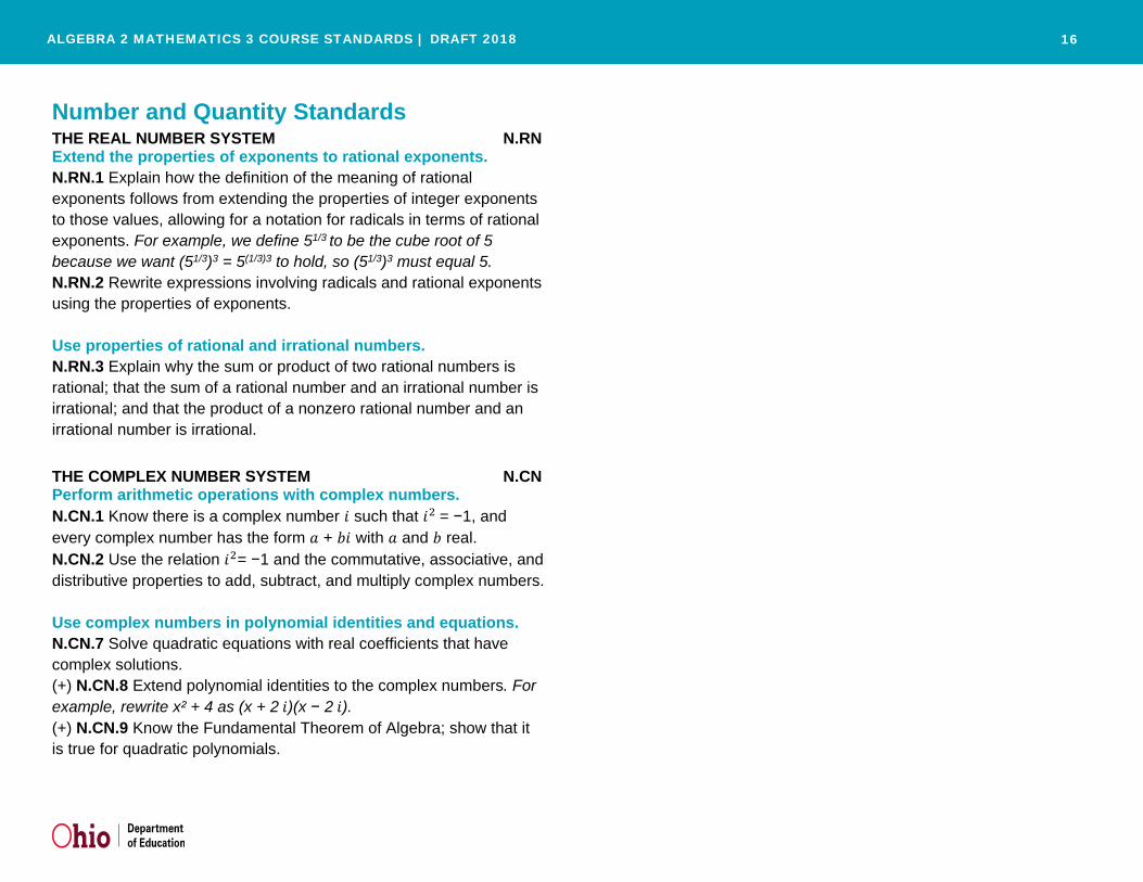
Number and Quantity Standards THE REAL NUMBER SYSTEM N.RN Extend the properties of exponents to rational exponents. N.RN.1 Explain how the definition of the meaning of rational exponents follows from extending the properties of integer exponents to those values, allowing for a notation for radicals in terms of rational exponents. For example, we define 51/3 to be the cube root of 5 because we want (51/3)3 = 5(1/3)3 to hold, so (51/3)3 must equal 5. N.RN.2 Rewrite expressions involving radicals and rational exponents using the properties of exponents. Use properties of rational and irrational numbers. N.RN.3 Explain why the sum or product of two rational numbers is rational; that the sum of a rational number and an irrational number is irrational; and that the product of a nonzero rational number and an irrational number is irrational.

THE COMPLEX NUMBER SYSTEM N.CN Perform arithmetic operations with complex numbers. N.CN.1 Know there is a complex number 𝑖𝑖 such that 𝑖𝑖2 = −1, and every complex number has the form 𝑎𝑎 + 𝑏𝑏𝑖𝑖 with 𝑎𝑎 and 𝑏𝑏 real. N.CN.2 Use the relation 𝑖𝑖2= −1 and the commutative, associative, and distributive properties to add, subtract, and multiply complex numbers. Use complex numbers in polynomial identities and equations. N.CN.7 Solve quadratic equations with real coefficients that have complex solutions. (+) N.CN.8 Extend polynomial identities to the complex numbers. For example, rewrite x² + 4 as (x + 2 𝑖𝑖)(x − 2 𝑖𝑖). (+) N.CN.9 Know the Fundamental Theorem of Algebra; show that it is true for quadratic polynomials.


17

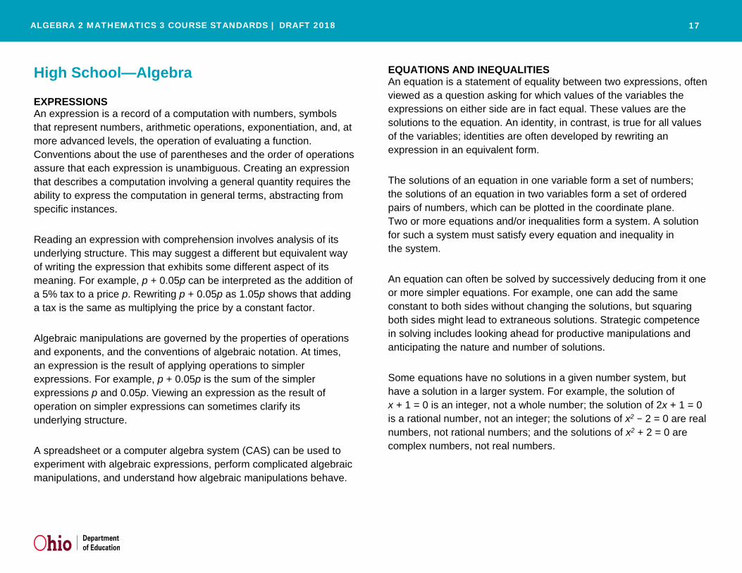
High School—Algebra EXPRESSIONS An expression is a record of a computation with numbers, symbols that represent numbers, arithmetic operations, exponentiation, and, at more advanced levels, the operation of evaluating a function. Conventions about the use of parentheses and the order of operations assure that each expression is unambiguous. Creating an expression that describes a computation involving a general quantity requires the ability to express the computation in general terms, abstracting from specific instances.

Reading an expression with comprehension involves analysis of its underlying structure. This may suggest a different but equivalent way of writing the expression that exhibits some different aspect of its meaning. For example, p + 0.05p can be interpreted as the addition of a 5% tax to a price p. Rewriting p + 0.05p as 1.05p shows that adding a tax is the same as multiplying the price by a constant factor.

Algebraic manipulations are governed by the properties of operations and exponents, and the conventions of algebraic notation. At times, an expression is the result of applying operations to simpler expressions. For example, p + 0.05p is the sum of the simpler expressions p and 0.05p. Viewing an expression as the result of operation on simpler expressions can sometimes clarify its underlying structure.

A spreadsheet or a computer algebra system (CAS) can be used to experiment with algebraic expressions, perform complicated algebraic manipulations, and understand how algebraic manipulations behave.

EQUATIONS AND INEQUALITIES An equation is a statement of equality between two expressions, often viewed as a question asking for which values of the variables the expressions on either side are in fact equal. These values are the solutions to the equation. An identity, in contrast, is true for all values of the variables; identities are often developed by rewriting an expression in an equivalent form.

The solutions of an equation in one variable form a set of numbers; the solutions of an equation in two variables form a set of ordered pairs of numbers, which can be plotted in the coordinate plane. Two or more equations and/or inequalities form a system. A solution for such a system must satisfy every equation and inequality in the system.

An equation can often be solved by successively deducing from it one or more simpler equations. For example, one can add the same constant to both sides without changing the solutions, but squaring both sides might lead to extraneous solutions. Strategic competence in solving includes looking ahead for productive manipulations and anticipating the nature and number of solutions.

Some equations have no solutions in a given number system, but have a solution in a larger system. For example, the solution of x + 1 = 0 is an integer, not a whole number; the solution of 2x + 1 = 0 is a rational number, not an integer; the solutions of x2 − 2 = 0 are real numbers, not rational numbers; and the solutions of x2 + 2 = 0 are complex numbers, not real numbers.


18

High School—Algebra, CONTINUED The same solution techniques used to solve equations can be used to rearrange formulas. For example, the formula for the area of a

trapezoid, A = ((𝑏𝑏1+𝑏𝑏2 )

2)h, can be solved for h using the same

deductive process.

Inequalities can be solved by reasoning about the properties of inequality. Many, but not all, of the properties of equality continue to hold for inequalities and can be useful in solving them.

CONNECTIONS WITH FUNCTIONS AND MODELING Expressions can define functions, and equivalent expressions define the same function. Asking when two functions have the same value for the same input leads to an equation; graphing the two functions allows for finding approximate solutions of the equation. Converting a verbal description to an equation, inequality, or system of these is an essential skill in modeling.


19

Algebra Standards SEEING STRUCTURE IN EXPRESSIONS A.SSE Interpret the structure of expressions. A.SSE.1. Interpret expressions that represent a quantity in terms of its context. ★

a. Interpret parts of an expression, such as terms, factors, and coefficients.

b. Interpret complicated expressions by viewing one or more of their parts as a single entity.

A.SSE.2 Use the structure of an expression to identify ways to rewrite it. For example, to factor 3x(x − 5) + 2(x − 5), students should recognize that the "x − 5" is common to both expressions being added, so it simplifies to (3x + 2)(x − 5); or see x4 − y4 as (x2)2 − (y2)2, thus recognizing it as a difference of squares that can be factored as (x2 − y2)(x2 + y2). Write expressions in equivalent forms to solve problems. A.SSE.3 Choose and produce an equivalent form of an expression to reveal and explain properties of the quantity represented by the expression.★

c. Use the properties of exponents to transform expressions for exponential functions. For example, 8t can be written as 23t.

(+) A.SSE.4 Derive the formula for the sum of a finite geometric series (when the common ratio is not 1), and use the formula to solve problems. For example, calculate mortgage payments.★

ARITHMETIC WITH POLYNOMIALS AND RATIONAL EXPRESSIONS A.APR Perform arithmetic operations on polynomials. A.APR.1 Understand that polynomials form a system analogous to the integers, namely, that they are closed under the operations of addition, subtraction, and multiplication; add, subtract, and multiply polynomials.

b. Extend to polynomial expressions beyond those expressions that simplify to forms that are linear or quadratic. (A2, M3)

Understand the relationship between zeros and factors of polynomials. A.APR.2 Understand and apply the Remainder Theorem: For a polynomial p(x) and a number a, the remainder on division by x − a is p(a). In particular, p(a) = 0 if and only if (x – a) is a factor of p(x). A.APR.3 Identify zeros of polynomials, when factoring is reasonable, and use the zeros to construct a rough graph of the function defined by the polynomial. Use polynomial identities to solve problems. A.APR.4 Prove polynomial identities and use them to describe numerical relationships. For example, the polynomial identity (x² + y²)² = (x² − y²)² + (2xy)² can be used to generate Pythagorean triples. (+) A.APR.5 Know and apply the Binomial Theorem for the expansion of (x + y)n in powers of x and y for a positive integer n, where x and y are any numbers. For example by using coefficients determined for by Pascal’s Triangle. The Binomial Theorem can be proved by mathematical induction or by a combinatorial argument.


20

Algebra Standards, CONTINUED ARITHMETIC WITH POLYNOMIALS AND RATIONAL EXPRESSIONS A.APR Rewrite rational expressions. A.APR.6 Rewrite simple rational expressionsG in different forms; write a(x)/b(x) in the form q(x) + r(x)/b(x), where a(x), b(x), q(x), and r(x) are polynomials with the degree of r(x) less than the degree of b(x), using inspection, long division, or, for the more complicated examples, a computer algebra system. (+) A.APR.7 Understand that rational expressions form a system analogous to the rational numbers, closed under addition, subtraction, multiplication, and division by a nonzero rational expression; add, subtract, multiply, and divide rational expressions.

CREATING EQUATIONS A.CED Create equations that describe numbers or relationships. A.CED.1 Create equations and inequalities in one variable and use them to solve problems. Include equations and inequalities arising from linear, quadratic, simple rational, and exponential functions. ★

c. Extend to include more complicated function situations with the option to solve with technology. (A2, M3)

A.CED.2 Create equations in two or more variables to represent relationships between quantities; graph equations on coordinate axes with labels and scales.★

c. Extend to include more complicated function situations with the option to graph with technology. (A2, M3)

A.CED.3 Represent constraints by equations or inequalities, and by systems of equations and/or inequalities, and interpret solutions as viable or non-viable options in a modeling context. For example, represent inequalities describing nutritional and cost constraints on combinations of different foods.★ (A1, M1)

a. While functions will often be linear, exponential, or quadratic, the types of problems should draw from more complicated situations. (A2, M3)

A.CED.4 Rearrange formulas to highlight a quantity of interest, using the same reasoning as in solving equations.★

d. While functions will often be linear, exponential, or quadratic, the types of problems should draw from more complicated situations. (A2, M3)

REASONING WITH EQUATIONS AND INEQUALITIES A.REI Understand solving equations as a process of reasoning and explain the reasoning. A.REI.2 Solve simple rational and radical equations in one variable, and give examples showing how extraneous solutions may arise. Solve systems of equations. A.REI.6 Solve systems of linear equations algebraically and graphically.

b. Extend to include solving systems of linear equations in three variables, but only algebraically. (A2, M3)

Represent and solve equations and inequalities graphically. A.REI.11 Explain why the x-coordinates of the points where the graphs of the equation y = f(x) and y = g(x) intersect are the solutions of the equation f(x) = g(x); find the solutions approximately, e.g., using technology to graph the functions, making tables of values, or finding successive approximations.


21

High School—Functions Functions describe situations where one quantity determines another. For example, the return on $10,000 invested at an annualized percentage rate of 4.25% is a function of the length of time the money is invested. Because we continually make theories about dependencies between quantities in nature and society, functions are important tools in the construction of mathematical models.

In school mathematics, functions usually have numerical inputs and outputs and are often defined by an algebraic expression. For example, the time in hours it takes for a car to drive 100 miles is a function of the car’s speed in miles per hour, v; the rule T(v) = 100/v expresses this relationship algebraically and defines a function whose name is T.

The set of inputs to a function is called its domain. We often infer the domain to be all inputs for which the expression defining a function has a value, or for which the function makes sense in a given context.

A function can be described in various ways, such as by a graph, e.g., the trace of a seismograph; by a verbal rule, as in, “I’ll give you a state, you give me the capital city;” by an algebraic expression like f(x) = a + bx; or by a recursive rule. The graph of a function is often a useful way of visualizing the relationship of the function models, and manipulating a mathematical expression for a function can throw light on the function’s properties.

Functions presented as expressions can model many important phenomena. Two important families of functions characterized by laws of growth are linear functions, which grow at a constant rate, and exponential functions, which grow at a constant percent rate. Linear functions with a constant term of zero describe proportional relationships.

A graphing utility or a computer algebra system can be used to experiment with properties of these functions and their graphs and to build computational models of functions, including recursively defined functions.

CONNECTIONS TO EXPRESSIONS, EQUATIONS, MODELING, AND COORDINATES. Determining an output value for a particular input involves evaluating an expression; finding inputs that yield a given output involves solving an equation. Questions about when two functions have the same value for the same input lead to equations, whose solutions can be visualized from the intersection of their graphs. Because functions describe relationships between quantities, they are frequently used in modeling. Sometimes functions are defined by a recursive process, which can be displayed effectively using a spreadsheet or other technology.


22

Functions Standards INTERPRETING FUNCTIONS F.IF Interpret functions that arise in applications in terms of the context. F.IF.4 For a function that models a relationship between two quantities, interpret key features of graphs and tables in terms of the quantities, and sketch graphs showing key features given a verbal description of the relationship. Key features include the following: intercepts; intervals where the function is increasing, decreasing, positive, or negative; relative maximums and minimums; symmetries; end behavior; and periodicity.★(A2, M3) F.IF.5 Relate the domain of a function to its graph and, where applicable, to the quantitative relationship it describes. For example, if the function h(n) gives the number of person-hours it takes to assemble n engines in a factory, then the positive integers would be an appropriate domain for the function.★

c. Emphasize the selection of a type of function for a model based on behavior of data and context. (A2, M3)

F.IF.6 Calculate and interpret the average rate of change of a function (presented symbolically or as a table) over a specified interval. Estimate the rate of change from a graph. ★ (A2, M3)

Analyze functions using different representations. F.IF.7 Graph functions expressed symbolically and indicate key features of the graph, by hand in simple cases and using technology for more complicated cases. Include applications and how key features relate to characteristics of a situation, making selection of a particular type of function model appropriate.★

c. Graph square root, cube root, and piecewise-defined functions, including step functions and absolute value functions. (A2, M3)

d. Graph polynomial functions, identifying zeros, when factoring is reasonable, and indicating end behavior. (A2, M3)

f. Graph exponential functions, indicating intercepts and end behavior, and trigonometric functions, showing period, midlineG, and amplitude. (A2, M3)

(+) g. Graph rational functions, identifying zeros and asymptotes when factoring is reasonable, and indicating end behavior. (A2, M3)

(+) h. Graph logarithmic functions, indicating intercepts and end behavior. (A2, M3)

F.IF.8 Write a function defined by an expression in different but equivalent forms to reveal and explain different properties of the function.

a. Use the process of factoring and completing the square in a quadratic function to show zeros, extreme values, and symmetry of the graph, and interpret these in terms of a context. (A2, M3)

b. Use the properties of exponents to interpret expressions for exponential functions. For example, identify percent rate of changeG in functions such as y = (1.02)t, and y = (0.97)t and classify them as representing exponential growth or decay. (A2, M3)

F.IF.9 Compare properties of two functions each represented in a different way (algebraically, graphically, numerically in tables, or by verbal descriptions). For example, given a graph of one quadratic function and an algebraic expression for another, say which has the larger maximum. (A2, M3)


23

Functions Standards, CONTINUED BUILDING FUNCTIONS F.BF Build a function that models a relationship between two quantities. F.BF.1 Write a function that describes a relationship between two quantities.★

b. Combine standard function types using arithmetic operations. For example, build a function that models the temperature of a cooling body by adding a constant function to a decaying exponential, and relate these functions to the model. (A2, M3)

Build new functions from existing functions. F.BF.3 Identify the effect on the graph of replacing f(x) by f(x) + k, kf(x), f(kx), and f(x + k) for specific values of k (both positive and negative); find the value of k given the graphs. Experiment with cases and illustrate an explanation of the effects on the graph using technology. Include recognizing even and odd functions from their graphs and algebraic expressions for them. (A2, M3) F.BF.4 Find inverse functions.

(+) b. Read values of an inverse function from a graph or a table, given that the function has an inverse. (A2, M3)

(+) c. Verify by composition that one function is the inverse of another. (A2, M3)

(+) d. Find the inverse of a function algebraically, given that the function has an inverse. (A2, M3)

LINEAR, QUADRATIC, AND EXPONENTIAL MODELS F.LE Construct and compare linear, quadratic, and exponential models, and solve problems. F.LE.4 For exponential models, express as a logarithm the solution to abct = d where a, c, and d are numbers and the base b is 2, 10, or e; evaluate the logarithm using technology.★

TRIGONOMETRIC FUNCTIONS F.TF Extend the domain of trigonometric functions using the unit circle. F.TF.1 Understand radian measure of an angle as the length of the arc on the unit circle subtended by the angle. F.TF.2 Explain how the unit circle in the coordinate plane enables the extension of trigonometric functions to all real numbers, interpreted as radian measures of angles traversed counterclockwise around the unit circle. Model periodic phenomena with trigonometric functions. F.TF.5 Choose trigonometric functions to model periodic phenomena with specified amplitude, frequency, and midline.★ Prove and apply trigonometric identities. F.TF.8 Prove the Pythagorean identity sin²(θ) + cos²(θ) = 1, and use it to find sin(θ), cos(θ), or tan(θ) given sin(θ), cos(θ), or tan(θ) and the quadrant of the angle.


24

High School—Geometry An understanding of the attributes and relationships of geometric objects can be applied in diverse contexts—interpreting a schematic drawing, estimating the amount of wood needed to frame a sloping roof, rendering computer graphics, or designing a sewing pattern for the most efficient use of material. Although there are many types of geometry, school mathematics is devoted primarily to plane Euclidean geometry, studied both synthetically (without coordinates) and analytically (with coordinates). Euclidean geometry is characterized most importantly by the Parallel Postulate, that through a point not on a given line there is exactly one parallel line. (Spherical geometry, in contrast, has no parallel lines.) During high school, students begin to formalize their geometry experiences from elementary and middle school, using more precise definitions and developing careful proofs. Later in college some students develop Euclidean and other geometries carefully from a small set of axioms. The concepts of congruence, similarity, and symmetry can be understood from the perspective of geometric transformation. Fundamental are the rigid motions: translations, rotations, reflections, and combinations of these, all of which are here assumed to preserve distance and angles (and therefore shapes generally). Reflections and rotations each explain a particular type of symmetry, and the symmetries of an object offer insight into its attributes— as when the reflective symmetry of an isosceles triangle assures that its base angles are congruent.

In the approach taken here, two geometric figures are defined to be congruent if there is a sequence of rigid motions that carries one onto the other. This is the principle of superposition. For triangles, congruence means the equality of all corresponding pairs of sides and all corresponding pairs of angles. During the middle grades, through experiences drawing triangles from given conditions, students notice ways to specify enough measures in a triangle to ensure that all triangles drawn with those measures are congruent. Once these triangle congruence criteria (ASA, SAS, and SSS) are established using rigid motions, they can be used to prove theorems about triangles, quadrilaterals, and other geometric figures. Similarity transformations (rigid motions followed by dilations) define similarity in the same way that rigid motions define congruence, thereby formalizing the similarity ideas of “same shape” and “scale factor” developed in the middle grades. These transformations lead to the criterion for triangle similarity that two pairs of corresponding angles are congruent. The definitions of sine, cosine, and tangent for acute angles are founded on right triangles and similarity, and, with the Pythagorean Theorem, are fundamental in many real-world and theoretical situations. The Pythagorean Theorem is generalized to non- right triangles by the Law of Cosines. Together, the Laws of Sines and Cosines embody the triangle congruence criteria for the cases where three pieces of information suffice to completely solve a triangle. Furthermore, these laws yield two possible solutions in the ambiguous case, illustrating that Side-Side-Angle is not a congruence criterion.


25

High School—Geometry, CONTINUED Analytic geometry connects algebra and geometry, resulting in powerful methods of analysis and problem solving. Just as the number line associates numbers with locations in one dimension, a pair of perpendicular axes associates pairs of numbers with locations in two dimensions. This correspondence between numerical coordinates and geometric points allows methods from algebra to be applied to geometry and vice versa. The solution set of an equation becomes a geometric curve, making visualization a tool for doing and understanding algebra. Geometric shapes can be described by equations, making algebraic manipulation into a tool for geometric understanding, modeling, and proof. Geometric transformations of the graphs of equations correspond to algebraic changes in their equations. Dynamic geometry environments provide students with experimental and modeling tools that allow them to investigate geometric phenomena in much the same way as computer algebra systems allow them to experiment with algebraic phenomena.

CONNECTIONS TO EQUATIONS The correspondence between numerical coordinates and geometric points allows methods from algebra to be applied to geometry and vice versa. The solution set of an equation becomes a geometric curve, making visualization a tool for doing and understanding algebra. Geometric shapes can be described by equations, making algebraic manipulation into a tool for geometric understanding, modeling, and proof.


26

Geometry Standards SIMILARITY, RIGHT TRIANGLES, AND TRIGONOMETRY Define trigonometric ratios, and solve problems involving right triangles. G.SRT.8 Solve problems involving right triangles.★ (+) b. Use trigonometric ratios and the Pythagorean Theorem to solve

right triangles in applied problems.★ (A2, M3)

Apply trigonometry to general triangles. (+) G.SRT.9 Derive the formula A = 1/2 ab sin(C) for the area of a triangle by drawing an auxiliary line from a vertex perpendicular to the opposite side. (+) G.SRT.10 Explain proofs of the Laws of Sines and Cosines and use the Laws to solve problems. (+) G.SRT.11 Understand and apply the Law of Sines and the Law of Cosines to find unknown measurements in right and non-right triangles, e.g., surveying problems, resultant forces.

CIRCLES G.C Find arc lengths and areas of sectors of circles. G.C.6 Derive formulas that relate degrees and radians, and convert between the two. (A2, M3)


27

High School—Statistics and Probablity Decisions or predictions are often based on data—numbers in context. These decisions or predictions would be easy if the data always sent a clear message, but the message is often obscured by variability. Statistics provides tools for describing variability in data and for making informed decisions that take it into account. Data are gathered, displayed, summarized, examined, and interpreted to discover patterns and deviations from patterns. Quantitative data can be described in terms of key characteristics: measures of shape, center, and spread. The shape of a data distribution might be described as symmetric, skewed, flat, or bell shaped, and it might be summarized by a statistic measuring center (such as mean or median) and a statistic measuring spread (such as standard deviation or interquartile range). Different distributions can be compared numerically using these statistics or compared visually using plots. Knowledge of center and spread are not enough to describe a distribution. Which statistics to compare, which plots to use, and what the results of a comparison might mean, depend on the question to be investigated and the real-life actions to be taken. Randomization has two important uses in drawing statistical conclusions. First, collecting data from a random sample of a population makes it possible to draw valid conclusions about the whole population, taking variability into account. Second, randomly assigning individuals to different treatments allows a fair comparison of the effectiveness of those treatments. A statistically significant outcome is one that is unlikely to be due to chance alone, and this can be evaluated only under the condition of randomness. The conditions under which data are collected are important in drawing conclusions from the data; in critically reviewing uses of statistics in public media and other reports, it is important to consider the study design, how the

data were gathered, and the analyses employed as well as the data summaries and the conclusions drawn. Random processes can be described mathematically by using a probability model: a list or description of the possible outcomes (the sample space), each of which is assigned a probability. In situations such as flipping a coin, rolling a number cube, or drawing a card, it might be reasonable to assume various outcomes are equally likely. In a probability model, sample points represent outcomes and combine to make up events; probabilities of events can be computed by applying the Addition and Multiplication Rules. Interpreting these probabilities relies on an understanding of independence and conditional probability, which can be approached through the analysis of two-way tables. Technology plays an important role in statistics and probability by making it possible to generate plots, regression functions, and correlation coefficients, and to simulate many possible outcomes in a short amount of time.

CONNECTIONS TO FUNCTIONS AND MODELING Functions may be used to describe data; if the data suggest a linear relationship, the relationship can be modeled with a regression line, and its strength and direction can be expressed through a correlation coefficient.


28

Statistics and Probability Standards INTERPRETING CATEGORICAL AND QUANTITATIVE DATA S.ID Summarize, represent, and interpret data on a single count or measurement variable. S.ID.4 Use the mean and standard deviation of a data set to fit it to a normal distribution and to estimate population percentages. Recognize that there are data sets for which such a procedure is not appropriate. Use calculators, spreadsheets, and tables to estimate areas under the normal curve.★ Summarize, represent, and interpret data on two categorical and quantitative variables. S.ID.6 Represent data on two quantitative variables on a scatter plot, and describe how the variables are related.★

a. Fit a function to the data; use functions fitted to data to solve problems in the context of the data. Use given functions, or choose a function suggested by the context. Emphasize linear, quadratic, and exponential models. (A2, M3)

b. Informally assess the fit of a function by discussing residuals. (A2, M3)

Interpret linear models. S.ID.9 Distinguish between correlation and causation.★

MAKING INFERENCES AND JUSTIFYING CONCLUSIONS S.IC Understand and evaluate random processes underlying statistical experiments. S.IC.1 Understand statistics as a process for making inferences about population parameters based on a random sample from that population.★ S.IC.2 Decide if a specified model is consistent with results from a given data-generating process, e.g., using simulation. For example, a model says a spinning coin falls heads up with probability 0.5. Would a result of 5 tails in a row cause you to question the model?★

MAKING INFERENCES AND JUSTIFYING CONCLUSIONS, CONT’D Make inferences and justify conclusions from sample surveys, experiments, and observational studies. S.IC.3 Recognize the purposes of and differences among sample surveys, experiments, and observational studies; explain how randomization relates to each.★ S.IC.4 Use data from a sample survey to estimate a population mean or proportion; develop a margin of error through the use of simulation models for random sampling.★ S.IC.5 Use data from a randomized experiment to compare two treatments; use simulations to decide if differences between sample statistics are statistically significant.★ S.IC.6 Evaluate reports based on data.★


29

__________________________________

1 Adapted from Wisconsin Department of Public Instruction, http://dpi.wi.gov/ standards/mathglos.html, accessed March 2, 2010.

2 Many different methods for computing quartiles are in use. The method defined here is sometimes called the Moore and McCabe method. See Langford, E., “Quartiles in Elementary Statistics,” Journal of Statistics Education Volume 14, Number 3 (2006). Glossary

Glossary Addition and subtraction within 5, 10, 20, 100, or 1000. Addition or subtraction of two whole numbers with whole number answers, and with sum or minuend in the range 0-5, 0-10, 0-20, or 0-100, respectively. Example: 8 + 2 = 10 is an addition within 10, 14 − 5 = 9 is a subtraction within 20, and 55 − 18 = 37 is a subtraction within 100.

Additive inverses. Two numbers whose sum is 0 are additive inverses of one another. Example: ¾ and − 3/4 are additive inverses of one another because ¾ + (−3/4) = (− 3/4) + 3/4 = 0.

Algorithm. See also: computation algorithm.

Associative property of addition. See Table 3 in this Glossary.

Associative property of multiplication. See Table 3 in this Glossary.

Bivariate data. Pairs of linked numerical observations. Example: a list of heights and weights for each player on a football team.

Box plot. A method of visually displaying a distribution of data values by using the median, quartiles, and extremes of the data set. A box shows the middle 50% of the data.1 See also: first quartile and third quartile.

Commutative property. See Table 3 in this Glossary.

Complex fraction. A fraction A/B where A and/or B are fractions (B nonzero).

Computation algorithm. A set of predefined steps applicable to a class of problems that gives the correct result in every case when the steps are carried out correctly. See also: computation strategy.

Computation strategy. Purposeful manipulations that may be chosen for specific problems, may not have a fixed order, and may be aimed at converting one problem into another. See also: computation algorithm.

Congruent. Two plane or solid figures are congruent if one can be obtained from the other by rigid motion (a sequence of rotations, reflections, and translations).

Counting on. A strategy for finding the number of objects in a group without having to count every member of the group. For example, if a stack of books is known to have 8 books and 3 more books are added to the top, it is not necessary to count the stack all over again. One can find the total by counting on—pointing to the top book and saying “eight,” following this with “nine, ten, eleven. There are eleven books now.”

Dilation. A transformation that moves each point along the ray through the point emanating from a fixed center, and multiplies distances from the center by a common scale factor.

Dot plot. See also: line plot.


30

__________________________________

3 Adapted from Wisconsin Department of Public Instruction, op. cit.


Expanded form. A multi-digit number is expressed in expanded form when it is written as a sum of single-digit multiples of powers of ten. For example, 643 = 600 + 40 + 3.

Expected value. For a random variable, the weighted average of its possible values, with weights given by their respective probabilities.

First quartile. For a data set with median M, the first quartile is the median of the data values less than M. Example: For the data set {1, 3, 6, 7, 10, 12, 14, 15, 22, 120}, the first quartile is 6.2 See also: median, third quartile, interquartile range.

Fluency. The ability to use efficient, accurate, and flexible methods for computing. Fluency does not imply timed tests.

Fluently. See also: fluency.

Fraction. A number expressible in the form a/b where a is a whole number and b is a positive whole number. (The word fraction in these standards always refers to a non-negative number.) See also: rational number.

Identity property of 0. See Table 3 in this Glossary.

Independently combined probability models. Two probability models are said to be combined independently if the probability of each ordered pair in the combined model equals the product of the original probabilities of the two individual outcomes in the ordered pair.

Integer. A number expressible in the form a or −a for some whole number a.

Interquartile Range. A measure of variation in a set of numerical data, the interquartile range is the distance between the first and third quartiles of the data set. Example: For the data set {1, 3, 6, 7, 10, 12, 14, 15, 22, 120}, the interquartile range is 15 − 6 = 9. See also: first quartile, third quartile.

Justify: To provide a convincing argument for the truth of a statement to a particular audience.

Line plot. A method of visually displaying a distribution of data values where each data value is shown as a dot or mark above a number line. Also known as a dot plot.3

Mean. A measure of center in a set of numerical data, computed by adding the values in a list and then dividing by the number of values in the list. (To be more precise, this defines the arithmetic mean) Example: For the data set {1, 3, 6, 7, 10, 12, 14, 15, 22, 120}, the mean is 21.

Mean absolute deviation. A measure of variation in a set of numerical data, computed by adding the distances between each data value and the mean, then dividing by the number of data values. Example: For the data set {2, 3, 6, 7, 10, 12, 14, 15, 22, 120}, the mean absolute deviation is 20.


31

__________________________________

Median. A measure of center in a set of numerical data. The median of a list of values is the value appearing at the center of a sorted version of the list—or the mean of the two central values, if the list contains an even number of values. Example: For the data set {2, 3, 6, 7, 10, 12, 14, 15, 22, 90}, the median is 11.

Midline. In the graph of a trigonometric function, the horizontal line halfway between its maximum and minimum values.

Multiplication and division within 100. Multiplication or division of two whole numbers with whole number answers, and with product or dividend in the range 0-100. Example: 72 ÷ 8 = 9.

Multiplicative inverses. Two numbers whose product is 1 are multiplicative inverses of one another. Example: 3/4

and 4/3 are multiplicative inverses of one another because 3/4 × 4/3 = 4/3 × 3/4 = 1.

Number line diagram. A diagram of the number line used to represent numbers and support reasoning about them. In a number line diagram for measurement quantities, the interval from 0 to 1 on the diagram represents the unit of measure for the quantity.

Percent rate of change. A rate of change expressed as a percent. Example: if a population grows from 50 to 55 in a year, it grows by 5/50 = 10% per year.

Probability distribution. The set of possible values of a random variable with a probability assigned to each.

Properties of operations. See Table 3 in this Glossary.

Properties of equality. See Table 4 in this Glossary.

Properties of inequality. See Table 5 in this Glossary.

Properties of operations. See Table 3 in this Glossary.

Probability. A number between 0 and 1 used to quantify likelihood for processes that have uncertain outcomes (such as tossing a coin, selecting a person at random from a group of people, tossing a ball at a target, or testing for a medical condition).

Probability model. A probability model is used to assign probabilities to outcomes of a chance process by examining the nature of the process. The set of all outcomes is called the sample space, and their probabilities sum to 1. See also: uniform probability model.

Prove: To provide a logical argument that demonstrates the truth of a statement. A proof is typically composed of a series of justifications, which are often single sentences, and may be presented informally or formally.

Random variable. An assignment of a numerical value to each outcome in a sample space.

Rational expression. A quotient of two polynomials with a nonzero denominator.


32

__________________________________


Rational number. A number expressible in the form a/b or −a/b for some fraction a/b. The rational numbers include the integers.

Rectilinear figure. A polygon all angles of which are right angles.

Rigid motion. A transformation of points in space consisting of a sequence of one or more translations, reflections, and/or rotations. Rigid motions are here assumed to preserve distances and angle measures.

Repeating decimal. The decimal form of a rational number. See also: terminating decimal.

Sample space. In a probability model for a random process, a list of the individual outcomes that are to be considered.

Scatter plot. A graph in the coordinate plane representing a set of bivariate data. For example, the heights and weights of a group of people could be displayed on a scatter plot.5

Similarity transformation. A rigid motion followed by a dilation.

Standard Algorithm. See computational algorithm

Tape diagram. A drawing that looks like a segment of tape, used to illustrate number relationships. Also known as a strip diagram, bar model, fraction strip, or length model.

Terminating decimal. A decimal is called terminating if its repeating digit is 0.

Third quartile. For a data set with median M, the third quartile is the median of the data values greater than M. Example: For the data set {2, 3, 6, 7, 10, 12, 14, 15, 22, 120}, the third quartile is 15. See also: median, first quartile, interquartile range.

Transitivity principle for indirect measurement. If the length of object A is greater than the length of object B, and the length of object B is greater than the length of object C, then the length of object A is greater than the length of object C. This principle applies to measurement of other quantities as well.

Trapezoid. 1. A trapezoid is a quadrilateral with at least one pair of parallel sides. (inclusive definition) 2. A trapezoid is a quadrilateral with exactly one pair of parallel sides. (exclusive definition) Districts may choose either

definition to use for instruction. Ohio's State Tests’ items will be written so that either definition will be acceptable.

Uniform probability model. A probability model which assigns equal probability to all outcomes. See also: probability model.

Vector. A quantity with magnitude and direction in the plane or in space, defined by an ordered pair or triple of real numbers.

Verify: To check the truth or correctness of a statement in specific cases.

Visual fraction model. A tape diagram, number line diagram, or area model.

Whole numbers. The numbers 0, 1, 2, 3, ….


33

Table 3. Properties of Operations. Here a, b and c stand for arbitrary numbers in a given number system. The properties of operations apply to the rational number system, the real number system and the complex number sytem.

ASSOCIATIVE PROPERTY OF ADDITION (𝑎𝑎 + 𝑏𝑏) + 𝑐𝑐 = 𝑎𝑎 + (𝑏𝑏 + 𝑐𝑐)

COMMUTATIVE PROPERTY OF ADDITION 𝑎𝑎 + 𝑏𝑏 = 𝑏𝑏 + 𝑎𝑎

ADDITIVE IDENTITY PROPERTY OF 0 𝑎𝑎 + 0 = 0 + 𝑎𝑎 = 𝑎𝑎

EXISTENCE OF ADDITIVE INVERSES For ever 𝑎𝑎 there exists −𝑎𝑎 so that 𝑎𝑎 + (−𝑎𝑎) = (−𝑎𝑎) + 𝑎𝑎 = 0

ASSOCIATIVE PROPERTY OF MULTIPLICATION (𝑎𝑎 × 𝑏𝑏) × 𝑐𝑐 = 𝑎𝑎 × (𝑏𝑏 × 𝑐𝑐)

COMMUTATIVE PROPERTY OF MULTIPLICATION 𝑎𝑎 × 𝑏𝑏 = 𝑏𝑏 × 𝑎𝑎

MULTIPLICATIVE IDENTITY PROPERTY OF 1 𝑎𝑎 × 1 = 1 × 𝑎𝑎 = 𝑎𝑎

EXISTENCE OF MULTIPLICATIVE INVERSES For every 𝑎𝑎 ≠ 0 there exists 1𝑎𝑎 so that 𝑎𝑎 × 1

𝑎𝑎= 1

𝑎𝑎× 𝑎𝑎 = 1

DISTRIBUTIVE PROPERTY OF MULTIPLICATION OVER ADDITION 𝑎𝑎 × (𝑏𝑏 + 𝑐𝑐) = 𝑎𝑎 × 𝑏𝑏 + 𝑎𝑎 × 𝑐𝑐 Table 4. Properties of Equality. Here a, b and c stand for arbitrary numbers in the rational, real or complex number sytems.

REFLEXIVE PROPERTY OF EQUALITY 𝑎𝑎 = 𝑎𝑎

SYMMETRIC PROPERTY OF EQUALITY If 𝑎𝑎 = 𝑏𝑏, then 𝑏𝑏 = 𝑎𝑎.

TRANSITIVE PROPERTY OF EQUALITY If 𝑎𝑎 = 𝑏𝑏 and 𝑏𝑏 = 𝑐𝑐, then 𝑎𝑎 = 𝑐𝑐.

ADDITION PROPERTY OF EQUALITY If 𝑎𝑎 = 𝑏𝑏, then 𝑎𝑎 + 𝑐𝑐 = 𝑏𝑏 + 𝑐𝑐.

SUBTRACTION PROPERTY OF EQUALITY If 𝑎𝑎 = 𝑏𝑏, then 𝑎𝑎 − 𝑐𝑐 = 𝑏𝑏 − 𝑐𝑐.

MULTIPLICATION PROPERTY OF EQUALITY If 𝑎𝑎 = 𝑏𝑏, then 𝑎𝑎 × 𝑐𝑐 = 𝑏𝑏 × 𝑐𝑐.

DIVISION PROPERTY OF EQUALITY If 𝑎𝑎 = 𝑏𝑏 and 𝑐𝑐 ≠ 0, then 𝑎𝑎 ÷ 𝑐𝑐 = 𝑏𝑏 ÷ 𝑐𝑐.

SUBSTITUTION PROPERTY OF EQUALITY If 𝑎𝑎 = 𝑎𝑎, then 𝑏𝑏 may be substituted for 𝑎𝑎 in any expression

containing 𝑎𝑎.


34

Table 5. Properties of Inequality. Here a, b and c stand for arbitrary numbers in the rational or real number sytem.

Exactly one of the following is true: 𝑎𝑎 < 𝑏𝑏, 𝑎𝑎 = 𝑏𝑏,𝑎𝑎 > 𝑏𝑏.

If 𝑎𝑎 > 𝑏𝑏 and 𝑏𝑏 > 𝑐𝑐, then 𝑎𝑎 > 𝑐𝑐.

If 𝑎𝑎 > 𝑏𝑏, then 𝑏𝑏 < 𝑎𝑎.

If 𝑎𝑎 > 𝑏𝑏, then −𝑎𝑎 < −𝑏𝑏.

If 𝑎𝑎 > 𝑏𝑏, then 𝑎𝑎 ± 𝑐𝑐 > 𝑏𝑏 ± 𝑐𝑐.

If 𝑎𝑎 > 𝑏𝑏 and 𝑐𝑐 > 0, then 𝑎𝑎 × 𝑐𝑐 > 𝑏𝑏 × 𝑐𝑐.

If 𝑎𝑎 > 𝑏𝑏 and 𝑐𝑐 < 0, then 𝑎𝑎 × 𝑐𝑐 < 𝑏𝑏 × 𝑐𝑐.

If 𝑎𝑎 > 𝑏𝑏 and 𝑐𝑐 > 0, then 𝑎𝑎 ÷ 𝑐𝑐 > 𝑏𝑏 ÷ 𝑐𝑐.

If 𝑎𝑎 > 𝑏𝑏 and 𝑐𝑐 < 0, then 𝑎𝑎 ÷ 𝑐𝑐 < 𝑏𝑏 ÷ 𝑐𝑐.


35

Acknowledgements ADVISORY COMMITTEE MEMBERS Aaron Altose The Ohio Mathematics Association of Two-Year Colleges Jeremy Beardmore Ohio Educational Service Center Association Jessica Burchett Ohio Teachers of English to Speakers of Other Languages Jeanne Cerniglia Ohio Education Association

Margie Coleman Cochair Jason Feldner Ohio Association for Career and Technical Education Brad Findell Ohio Higher Education Gregory D. Foley Ohio Mathematics and Science Coalition Margaret (Peggy) Kasten Cochair

Courtney Koestler Ohio Mathematics Education Leadership Council Scott Mitter Ohio Math and Science Supervisors Tabatha Nadolny Ohio Federation of Teachers Eydie Schilling Ohio Association for Supervision and Curriculum Development Kim Yoak Ohio Council of Teachers of Mathematics


36

WORKING GROUP MEMBERS Darry Andrews Higher Education, Ohio State University, C Bridgette Beeler Teacher, Perrysburg Exempted Local, NW Melissa Bennett Teacher, Minford Local, SE Dawn Bittner Teacher, Cincinnati Public Schools, SW Katherine Bunsey Teacher, Lakewood City, NE Hoyun Cho Higher Education, Capital University, C Viki Cooper Curriculum Specialist/Coordinator, Pickerington Local, C Ali Fleming Teacher, Bexley City, C Linda Gillum Teacher, Springboro City Schools, SW Gary Herman Curriculum Specialist/Coordinator, Putnam County ESC, NW William Husen Higher Education, Ohio State University, C Kristen Kelly Curriculum Specialist/Coordinator, Cleveland Metropolitan School District, NE Endora Kight Neal Curriculum Specialist/Coordinator, Cleveland Metropolitan School District, NE

Julie Kujawa Teacher, Oregon City, NW Sharilyn Leonard Teacher, Oak Hill Union Local Schools, SE Michael Lipnos Curriculum Specialist/Coordinator, Aurora City, NE Dawn Machacek Teacher, Toledo Public Schools, NW Janet McGuire Teacher, Gallia County Schools, SE Jill Madonia Curriculum Specialist/Coordinator, Akron Public Schools, NE Cindy McKinstry Teacher, East Palestine City, NE Cindy Miller Curriculum Specialist/Coordinator, Maysville Local, SE Anita O’Mellan Higher Education, Youngstown State University, NE Sherryl Proctor Teacher, Vantage Career Center, NW Diane Reisdorff Teacher, Westlake City, NE Susan Rice Teacher, Mount Vernon City, C Tess Rivero Teacher, Bellbrook-Sugarcreek Schools, SW

Benjamin Shaw Curriculum Specialist/Coordinator, Mahoning County ESC, NE Julia Shew Higher Education, Columbus State Community College, C Tiffany Sibert Teacher, Lima Shawnee Local, NW Jennifer Statzer Principal, Greenville City, SW Karma Vince Teacher, Sylvania City, NW Jennifer Walls Teacher, Akron Public Schools, NE Gaynell Wamer Teacher, Toledo City, NW Victoria Warner Teacher, Greenville City, SW Mary Webb Teacher, North College Hill, SW Barb Weidus Curriculum Specialist/Coordinator, New Richmond Exempted Village, SW Sandra Wilder Teacher, Akron Public Schools, NE Tong Yu Teacher,Cincinnati Public Schools, SW

ohio’s learning standards mathematics

Documents