om research: from problem driven to data driven...
TRANSCRIPT
OM Research: From Problem Driven to
Data Driven Research
David Simchi-Levi
E-mail: [email protected]
1

Meir Rosenblatt Memorial Lecture
2

3
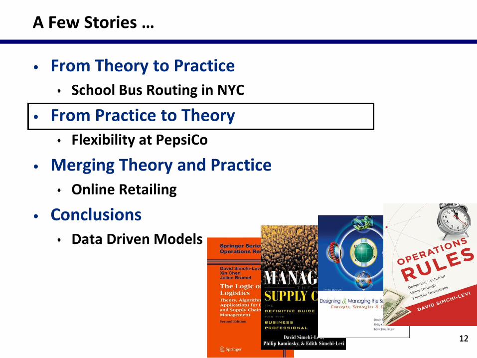
A Few Stories …
• From Theory to Practice
School Bus Routing in NYC
• From Practice to Theory
Flexibility at PepsiCo
• Merging Theory and Practice
Online Retailing
• Conclusions
Data Driven Models
4
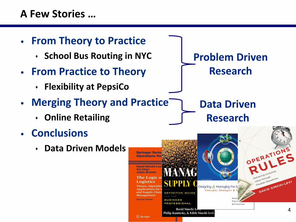
A Few Stories …
• From Theory to Practice
School Bus Routing in NYC
• From Practice to Theory
Flexibility at PepsiCo
• Merging Theory and Practice
Online Retailing
• Conclusions
Data Driven Models
Problem Driven Research
Data Driven Research

5
A Few Stories …
• From Theory to Practice
School Bus Routing in NYC
• From Practice to Theory
Flexibility at PepsiCo
• Merging Theory and Practice
Online Retailing
• Conclusions
Data Driven Models
5
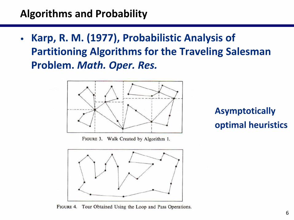
Algorithms and Probability
• Karp, R. M. (1977), Probabilistic Analysis of Partitioning Algorithms for the Traveling Salesman Problem. Math. Oper. Res.
6
Asymptotically
optimal heuristics
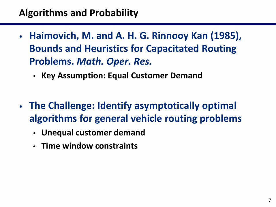
Algorithms and Probability
• Haimovich, M. and A. H. G. Rinnooy Kan (1985), Bounds and Heuristics for Capacitated Routing Problems. Math. Oper. Res.
Key Assumption: Equal Customer Demand
• The Challenge: Identify asymptotically optimal algorithms for general vehicle routing problems
Unequal customer demand
Time window constraints
7
General Vehicle Routing Problems
8
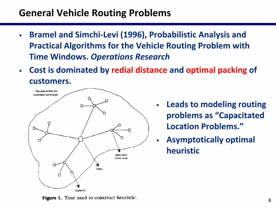
• Bramel and Simchi-Levi (1996), Probabilistic Analysis and Practical Algorithms for the Vehicle Routing Problem with Time Windows. Operations Research
• Cost is dominated by redial distance and optimal packing of customers.
• Leads to modeling routing problems as “Capacitated Location Problems.”
• Asymptotically optimal heuristic
Weaknesses and Strengths
• Two very strong assumptions
Large size problems
Independent customer behavior
• Provides insight into the structure of efficient algorithms:
Cost and Service
Computational time
9
NYC--School Bus Routing System
10
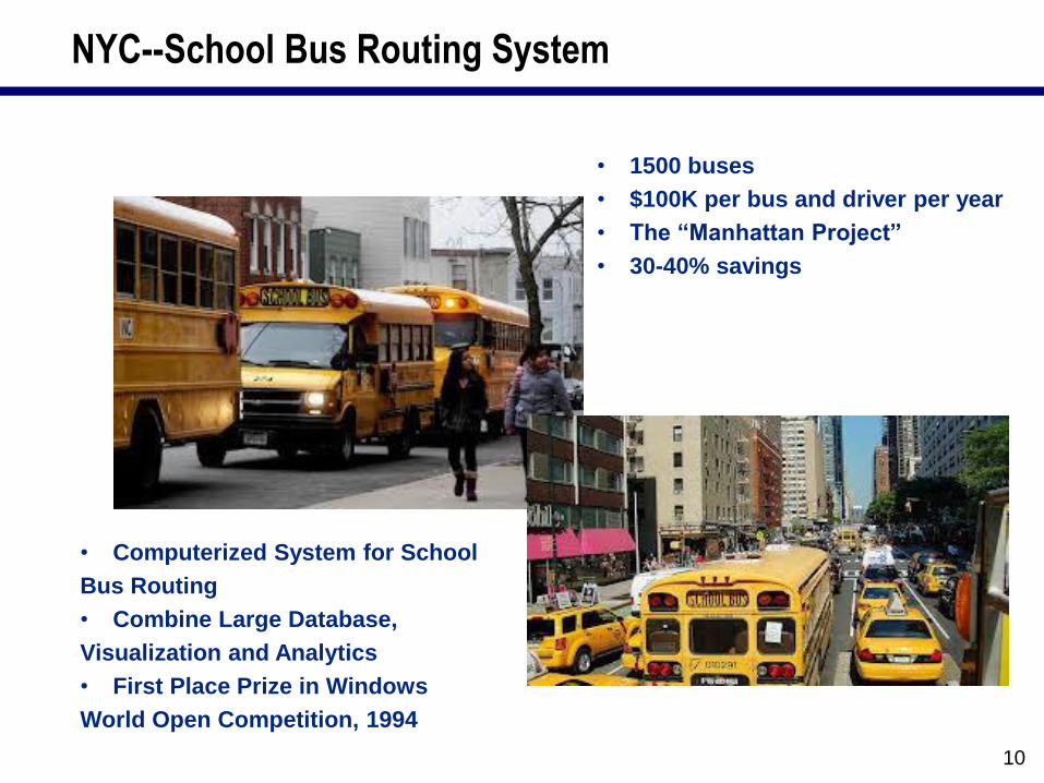
• Computerized System for School
Bus Routing
• Combine Large Database,
Visualization and Analytics
• First Place Prize in Windows
World Open Competition, 1994
• 1500 buses
• $100K per bus and driver per year
• The “Manhattan Project”
• 30-40% savings
Confidential
LogicTools, Inc. – Corporate Overview
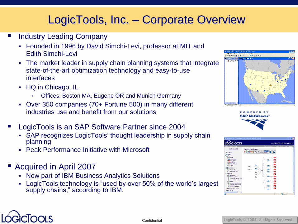
Industry Leading Company
Founded in 1996 by David Simchi-Levi, professor at MIT and Edith Simchi-Levi
The market leader in supply chain planning systems that integrate state-of-the-art optimization technology and easy-to-use interfaces
HQ in Chicago, IL
• Offices: Boston MA, Eugene OR and Munich Germany
Over 350 companies (70+ Fortune 500) in many different industries use and benefit from our solutions
LogicTools is an SAP Software Partner since 2004 SAP recognizes LogicTools’ thought leadership in supply chain
planning
Peak Performance Initiative with Microsoft
Acquired in April 2007 Now part of IBM Business Analytics Solutions
LogicTools technology is “used by over 50% of the world’s largest supply chains,” according to IBM.
12
A Few Stories …
• From Theory to Practice
School Bus Routing in NYC
• From Practice to Theory
Flexibility at PepsiCo
• Merging Theory and Practice
Online Retailing
• Conclusions
Data Driven Models
12
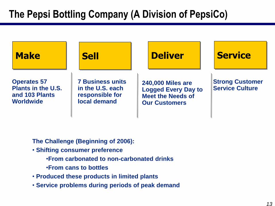
The Pepsi Bottling Company (A Division of PepsiCo)
Operates 57 Plants in the U.S. and 103 Plants Worldwide
7 Business units in the U.S. each responsible for local demand
240,000 Miles are Logged Every Day to Meet the Needs of Our Customers
Strong Customer Service Culture
Make Sell Deliver Service
The Challenge (Beginning of 2006):
• Shifting consumer preference
•From carbonated to non-carbonated drinks
•From cans to bottles
• Produced these products in limited plants
• Service problems during periods of peak demand
13
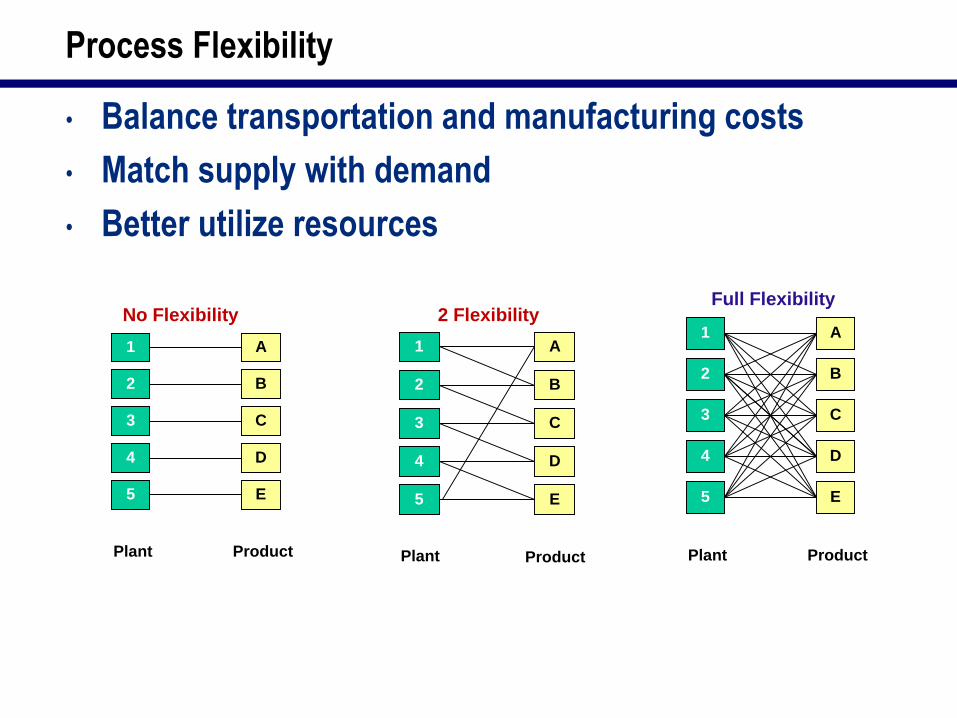
Process Flexibility
• Balance transportation and manufacturing costs
• Match supply with demand
• Better utilize resources
1 A
ProductPlant
2 B
3 C
4 D
5 E
No Flexibility
1 A
ProductPlant
2 B
3 C
4 D
5 E
2 Flexibility1 A
ProductPlant
2 B
3 C
4 D
5 E
Full Flexibility

Chaining Strategy (Jordan & Graves 1995)
• Focus: maximize the amount of demand satisfied
• Simulation study
15
1 A
ProductPlant
2 B
3 C
4 D
5 E
Short chains
1 A
ProductPlant
2 B
3 C
4 D
5 E
Long chain1 A
ProductPlant
2 B
3 C
4 D
5 E
Full Flexibility
~<
6 F 6 F 6 F
Applications to different settings:
[Sheikhzadeh et al. 1998], [Graves & Tomlin 2003], [Hopp et al. 2004],
[Gurumurthi & Benjaafar 2004], [Bish et al. 2005], [Iravani et al. 2005],
[Wallace & Whitt 2005], [Chou et al. 2010a]

PepsiCo’s Press Release, 2008—The Impact
• Creation of regular meetings bringing together Supply chain,
Transport, Finance, Sales and Manufacturing functions to discuss
sourcing and pre-build strategies
• Reduction in raw material and supplies inventory from $201 to $195
million
• A 2 percentage point decline in in growth of transport miles even as
revenue grew
• An additional 12.3 million cases available to be sold due to
reduction in warehouse out-of-stock levels
To put the last result in perspective, the reduction in warehouse out-of-stock levels
effectively added one and a half production lines worth of capacity to the firm’s
supply chain without any capital expenditure.
16
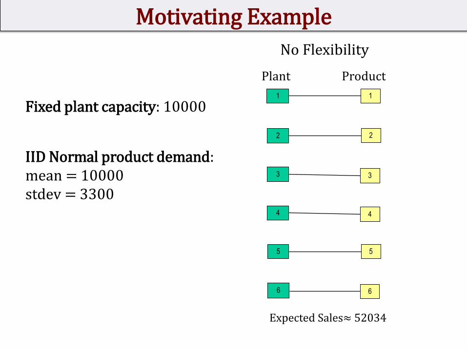
Motivating Example
Fixed plant capacity: 10000
IID Normal product demand: mean = 10000stdev = 3300
1 1
2 2
3 3
4 4
5 5
6 6
Plant Product
Expected Sales≈ 52034
No Flexibility
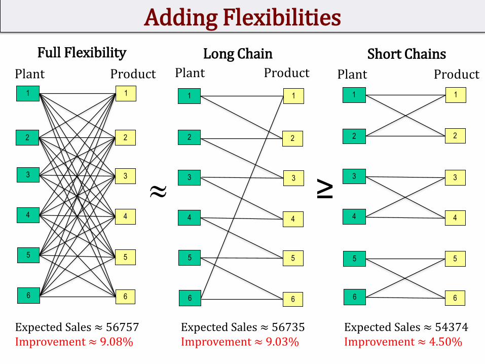
Adding Flexibilities
1 1
2 2
3 3
4 4
5 5
6 6
Plant Product
Expected Sales ≈ 56757Improvement ≈ 9.08%
Full Flexibility
1 1
2 2
3 3
4 4
5 5
6 6
Plant Product
Expected Sales ≈ 56735Improvement ≈ 9.03%
Long Chain
1 1
2 2
3 3
4 4
5 5
6 6
Plant Product
Expected Sales ≈ 54374Improvement≈ 4.50%
Short Chains
≥
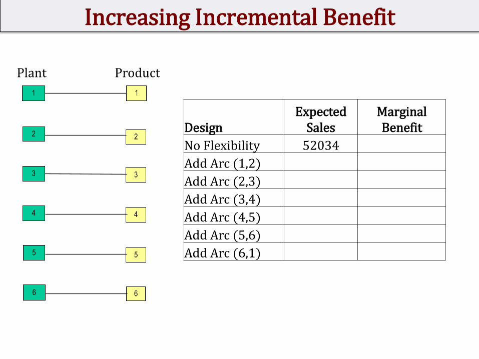
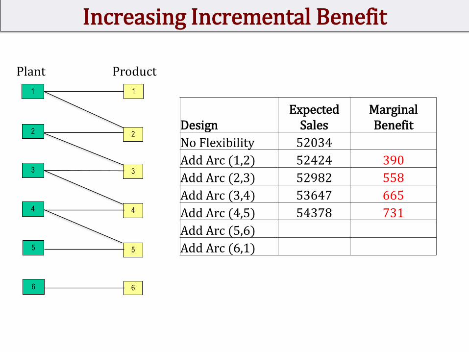
Increasing Incremental Benefit
1 1
2 2
3 3
4 4
5 5
6 6
Plant Product
DesignExpected
SalesMarginal Benefit
No Flexibility 52034
Add Arc (1,2)
Add Arc (2,3)
Add Arc (3,4)
Add Arc (4,5)
Add Arc (5,6)
Add Arc (6,1)
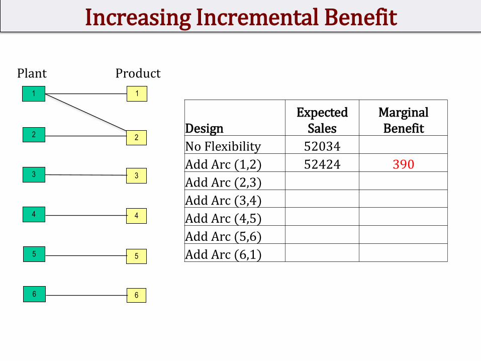
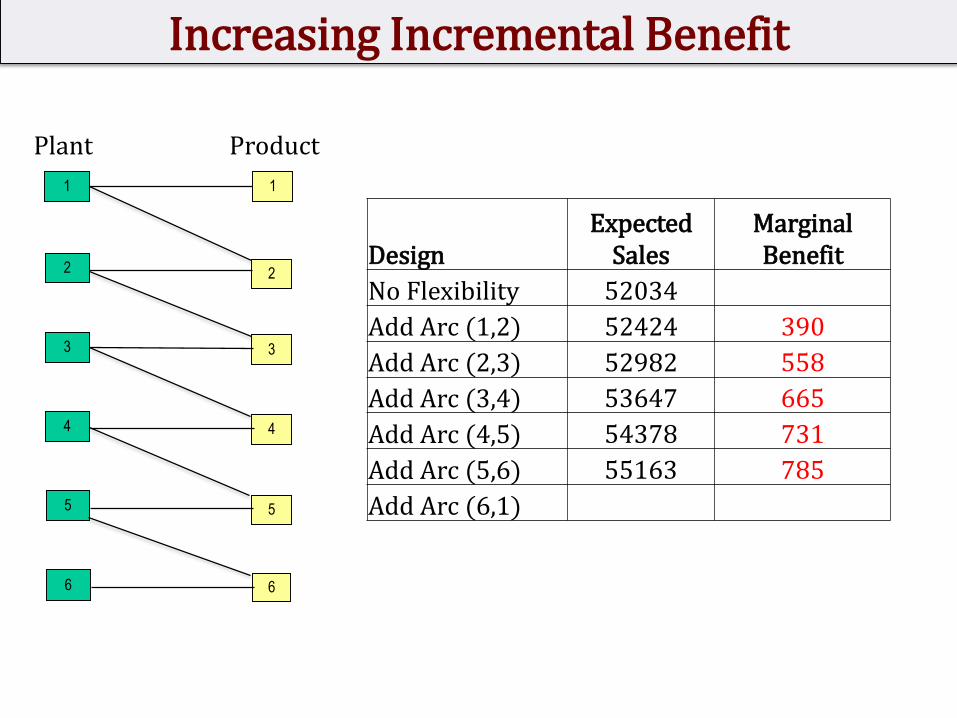
Increasing Incremental Benefit
1 1
2 2
3 3
4 4
5 5
6 6
Plant Product
DesignExpected
SalesMarginal Benefit
No Flexibility 52034
Add Arc (1,2) 52424 390
Add Arc (2,3)
Add Arc (3,4)
Add Arc (4,5)
Add Arc (5,6)
Add Arc (6,1)

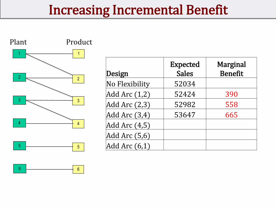
Increasing Incremental Benefit
1 1
2 2
3 3
4 4
5 5
6 6
Plant Product
DesignExpected
SalesMarginal Benefit
No Flexibility 52034
Add Arc (1,2) 52424 390
Add Arc (2,3) 52982 558
Add Arc (3,4)
Add Arc (4,5)
Add Arc (5,6)
Add Arc (6,1)
Increasing Incremental Benefit
1 1
2 2
3 3
4 4
5 5
6 6
Plant Product
DesignExpected
SalesMarginal Benefit
No Flexibility 52034
Add Arc (1,2) 52424 390
Add Arc (2,3) 52982 558
Add Arc (3,4) 53647 665
Add Arc (4,5)
Add Arc (5,6)
Add Arc (6,1)
Increasing Incremental Benefit
1 1
2 2
3 3
4 4
5 5
6 6
Plant Product
DesignExpected
SalesMarginal Benefit
No Flexibility 52034
Add Arc (1,2) 52424 390
Add Arc (2,3) 52982 558
Add Arc (3,4) 53647 665
Add Arc (4,5) 54378 731
Add Arc (5,6)
Add Arc (6,1)
Increasing Incremental Benefit
1 1
2 2
3 3
4 4
5 5
6 6
Plant Product
DesignExpected
SalesMarginal Benefit
No Flexibility 52034
Add Arc (1,2) 52424 390
Add Arc (2,3) 52982 558
Add Arc (3,4) 53647 665
Add Arc (4,5) 54378 731
Add Arc (5,6) 55163 785
Add Arc (6,1)
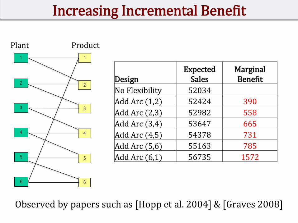
Increasing Incremental Benefit
1 1
2 2
3 3
4 4
5 5
6 6
Plant Product
DesignExpected
SalesMarginal Benefit
No Flexibility 52034
Add Arc (1,2) 52424 390
Add Arc (2,3) 52982 558
Add Arc (3,4) 53647 665
Add Arc (4,5) 54378 731
Add Arc (5,6) 55163 785
Add Arc (6,1) 56735 1572

Flexibility Structures
1 1
2 2
3 3
4 4
1 1
2 2
3 3
4 4
Cn Fn
Long Chain Full Flexibility
• Assumptions : # plants =# products; plant capacity is 1• Notations: For a demand realization d, we use P(d, A) to denote
the sales of flexibility structure A
Ln
1
2
3
4
1
2
3
4
Open Chain
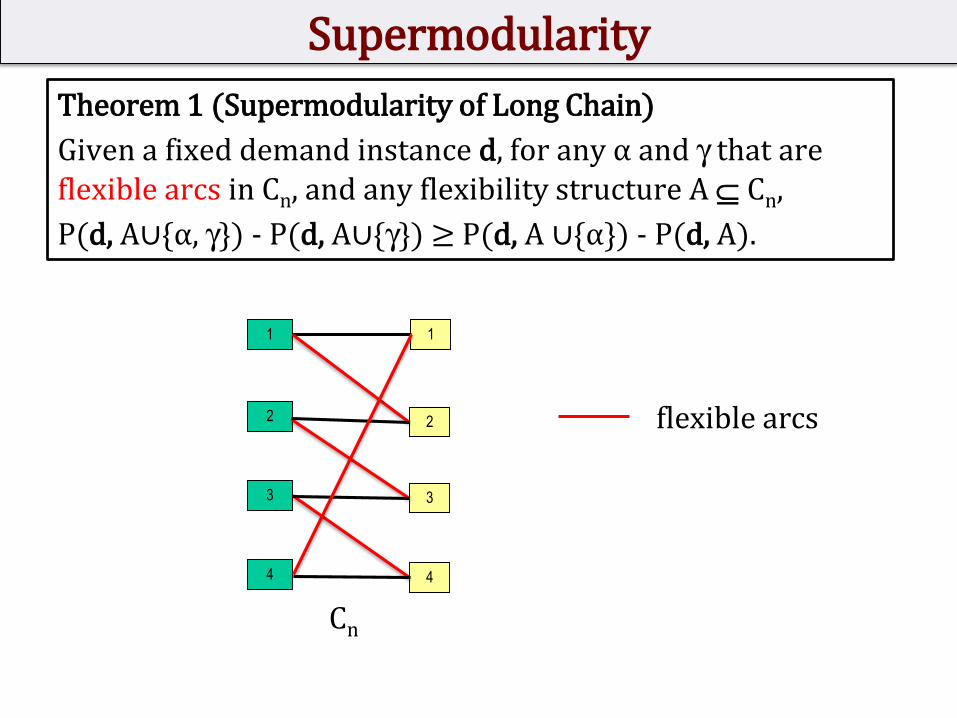
Supermodularity
Theorem 1 (Supermodularity of Long Chain)
Given a fixed demand instance d, for any α and g that are flexible arcs in Cn, and any flexibility structure A Cn,
P(d, A∪{α, g}) - P(d, A∪{g}) ≥ P(d, A ∪{α}) - P(d, A).
1 1
2 2
3 3
4 4
Cn
flexible arcs

Supermodularity
Theorem 1 (Supermodularity of Long Chain)
Given a fixed demand instance d, for any α and g that are flexible arcs in Cn, and any flexibility structure A Cn,
P(d, A∪{α, g}) - P(d, A∪{g}) ≥ P(d, A ∪{α}) - P(d, A).
• P(d, A ∪{α}) - P(d, A)
• increase in sales when we add α to A.
• P(d, A∪{α, g}) - P(d, A∪{g}):
• increase in sales when we add α to A∪{g}.

Supermodularity
Theorem 1 (Supermodularity of Long Chain)
Given a fixed demand instance d, for any α and g that are flexible arcs in Cn, and any flexibility structure A Cn,
P(d, A∪{α, g}) - P(d, A∪{g}) ≥ P(d, A ∪{α}) - P(d, A).
Application of [Gale and Politof 1981].
Corollary 1 (Increasing in Marginal Benefits)
The marginal benefits as the long chain is constructed is always increasing.
Observed by papers such as [Hopp et al. 2004] & [Graves 2008]
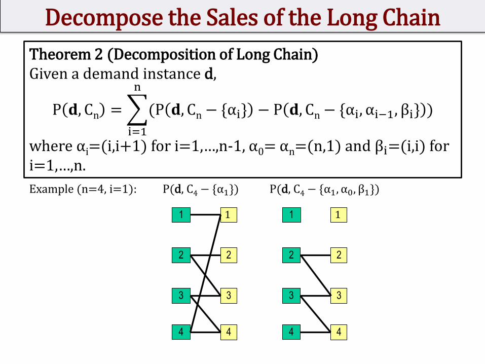
Decompose the Sales of the Long Chain
Theorem 2 (Decomposition of Long Chain)Given a demand instance d,
P 𝐝, Cn =
i=1
n
(P 𝐝, Cn− {αi} − P 𝐝, Cn− {αi, αi−1, βi} )
where αi=(i,i+1) for i=1,…,n-1, α0= αn=(n,1) and βi=(i,i) for i=1,…,n.
1 1
2 2
3 3
4 4
P(d, C4− {α1}) P(d, C4− {α1, α0, β1})
1 1
2 2
3 3
4 4
Example (n=4, i=1):
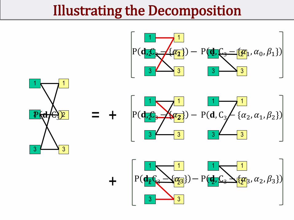
Illustrating the Decomposition
1 1
2 2
3 3
1 1
2 2
3 3
1 1
2 2−
1 1
2 2
3 3
2 2
3 3
−
1 1
2 2
3 3
1 1
3 3
−= +
+
P 𝐝, C3
P 𝐝, C3− {𝛼1}
P 𝐝, C3− {𝛼2}
P 𝐝, C3− {𝛼3}
P 𝐝, C3− {𝛼1, 𝛼0, 𝛽1}
P 𝐝, C3− {𝛼2, 𝛼1, 𝛽2}
P 𝐝, C3 − {𝛼3, 𝛼2, 𝛽3}

Key Idea of the Proof
1 1
2 2
3 3
1 1
2 2
3 3
1 1
2 2
1 1
2 2
3 3
2 2
3 3
1 1
2 2
3 3
1 1
3 3
= +
+ −
−
−

Under IID Demand
1 1
2 2
3 3
1 1
2 2
3 3
2 2
3 3
1 1
2 2
3 3
1 1
3 3
= +
+1 1
2 2
3 3
1 1
2 2−
−
−
Under IID demand,
= =
3X
E[P(D, L3)] E[P(D, L2)]
E[P(D, C3)]
Proposition 1 (Expected Performance of Long Chain)For IID demand, E[P(D, Cn)]/n = E[P(D, Ln)– P(D, Ln-1)].
= =
( )
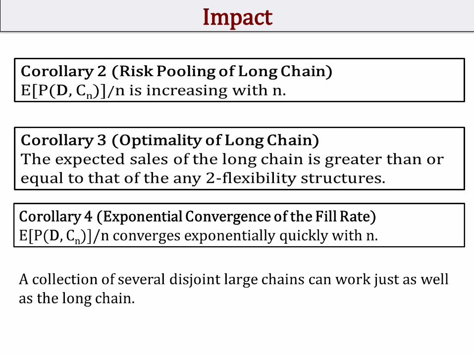
Impact
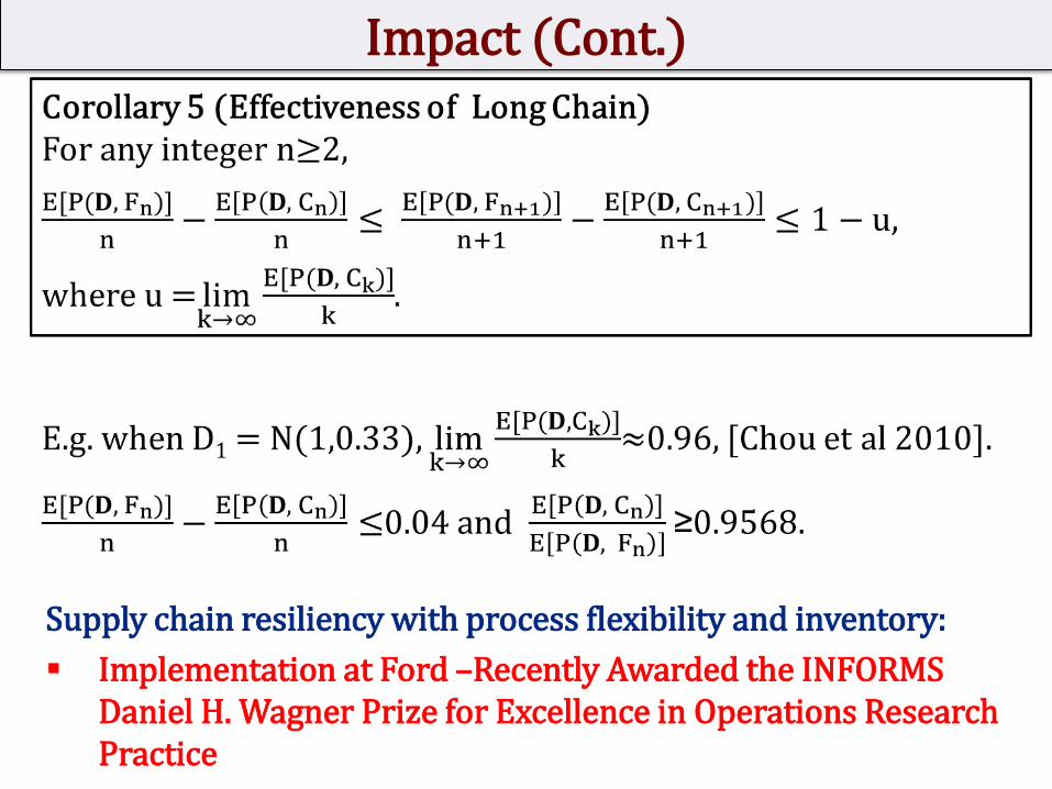
Impact (Cont.)
Supply chain resiliency with process flexibility and inventory:
Implementation at Ford –Recently Awarded the INFORMS Daniel H. Wagner Prize for Excellence in Operations Research Practice
36
A Few Stories …
• From Theory to Practice
School Bus Routing in NYC
• From Practice to Theory
Flexibility at PepsiCo
• Merging Theory and Practice
Online Retailing
• Conclusions
Data Driven Models
36
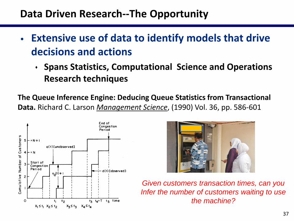
Data Driven Research--The Opportunity
• Extensive use of data to identify models that drive decisions and actions
Spans Statistics, Computational Science and Operations Research techniques
37
The Queue Inference Engine: Deducing Queue Statistics from Transactional Data. Richard C. Larson Management Science, (1990) Vol. 36, pp. 586-601
Given customers transaction times, can you
Infer the number of customers waiting to use
the machine?
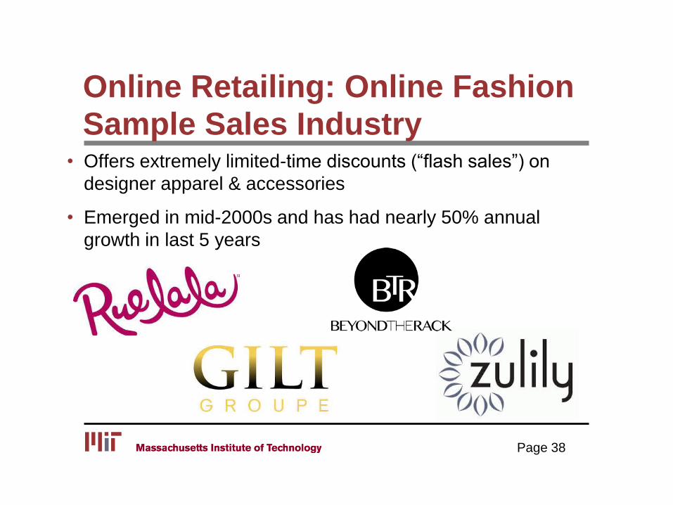
Online Retailing: Online Fashion
Sample Sales Industry• Offers extremely limited-time discounts (“flash sales”) on
designer apparel & accessories
• Emerged in mid-2000s and has had nearly 50% annual
growth in last 5 years
Page 38

Page 39
Snapshot of Rue La La’s Website

“Style”
Page 40

“SKU”
Page 41
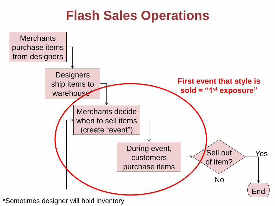
Flash Sales Operations
Merchants
purchase items
from designers
Designers
ship items to
warehouse*
Merchants decide
when to sell items
(create “event”)
During event,
customers
purchase items
Sell out
of item?
End
*Sometimes designer will hold inventory
Yes
No
First event that style is
sold = “1st exposure”
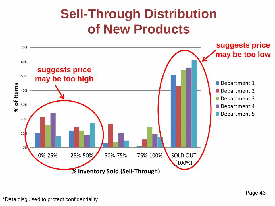
*Data disguised to protect confidentiality
0%
10%
20%
30%
40%
50%
60%
70%
0%-25% 25%-50% 50%-75% 75%-100% SOLD OUT(100%)
% o
f It
em
s
% Inventory Sold (Sell-Through)
1st Exposure Sell-Through Distribution
Department 1
Department 2
Department 3
Department 4
Department 5
Sell-Through Distribution
of New Products
Page 43
suggests price
may be too low
suggests price
may be too high
Page 44
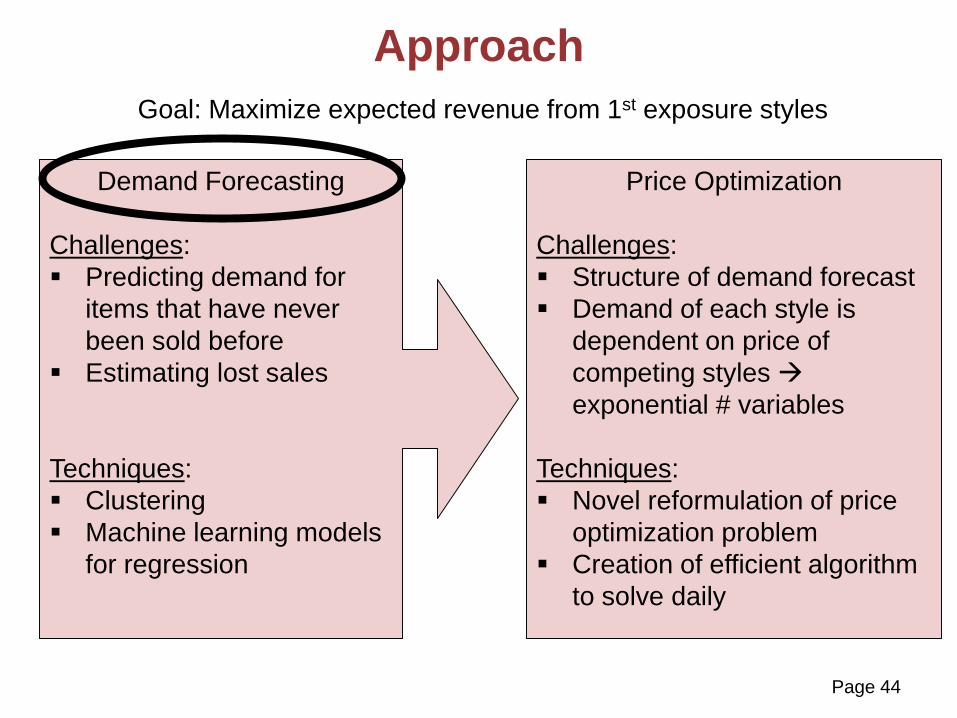
Approach
Goal: Maximize expected revenue from 1st exposure styles
Demand Forecasting
Challenges:
Predicting demand for
items that have never
been sold before
Estimating lost sales
Techniques:
Clustering
Machine learning models
for regression
Price Optimization
Challenges:
Structure of demand forecast
Demand of each style is
dependent on price of
competing styles
exponential # variables
Techniques:
Novel reformulation of price
optimization problem
Creation of efficient algorithm
to solve daily
Page 45
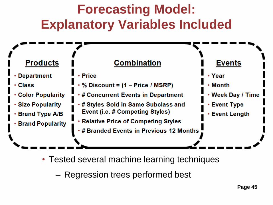
Forecasting Model:
Explanatory Variables Included
• Tested several machine learning techniques
– Regression trees performed best

Regression Tree – Illustration
Page 46
Demand
prediction
If condition is true, move left;
otherwise, move right
Page 47
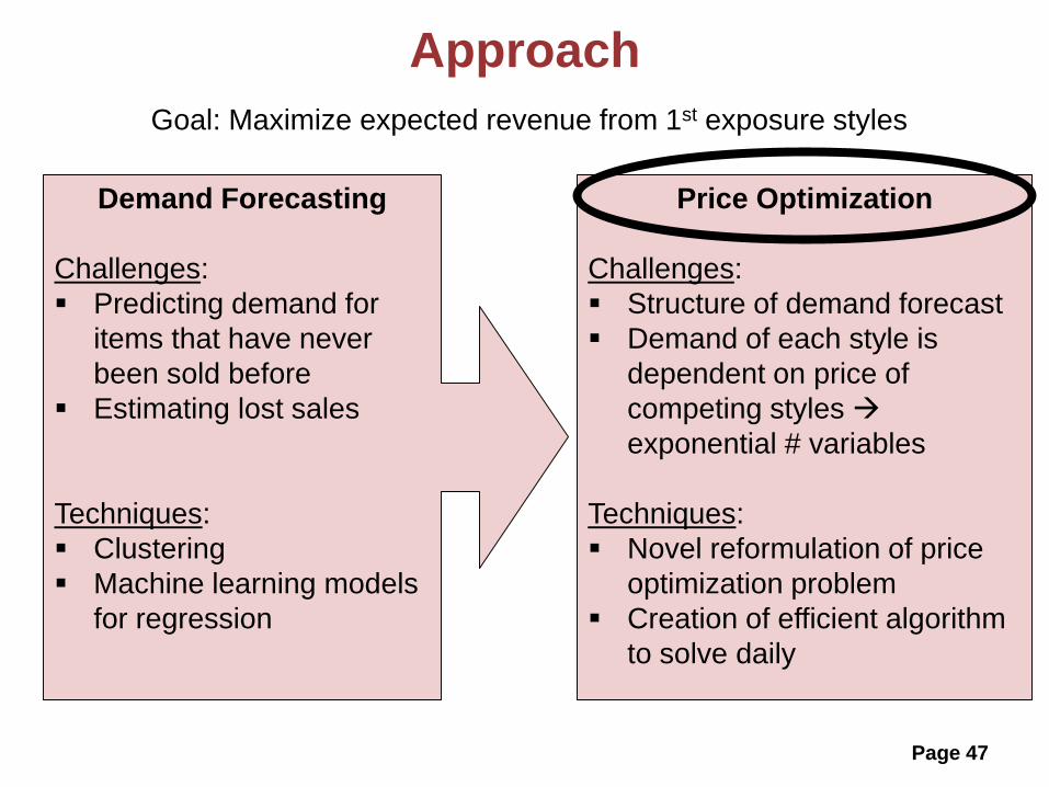
Approach
Goal: Maximize expected revenue from 1st exposure styles
Demand Forecasting
Challenges:
Predicting demand for
items that have never
been sold before
Estimating lost sales
Techniques:
Clustering
Machine learning models
for regression
Price Optimization
Challenges:
Structure of demand forecast
Demand of each style is
dependent on price of
competing styles
exponential # variables
Techniques:
Novel reformulation of price
optimization problem
Creation of efficient algorithm
to solve daily

Price Optimization Complexity
• Three features used to predict demand are associated with pricing
– Price
– % Discount =
– Relative Price of Competing Styles =
• Pricing must be optimized concurrently for all competing styles
– Would be impractical to calculate revenue for all potential
combinations of prices
• We developed an efficient algorithm to solve on a daily basis
Page 48
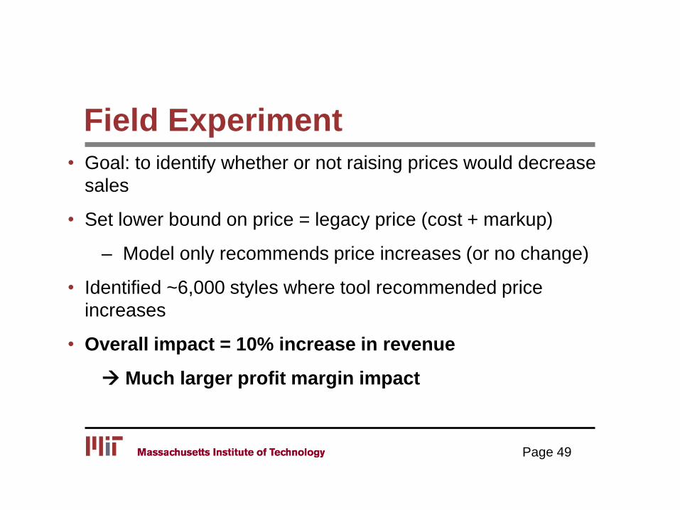
Field Experiment
• Goal: to identify whether or not raising prices would decrease
sales
• Set lower bound on price = legacy price (cost + markup)
– Model only recommends price increases (or no change)
• Identified ~6,000 styles where tool recommended price
increases
• Overall impact = 10% increase in revenue
Much larger profit margin impact
Page 49
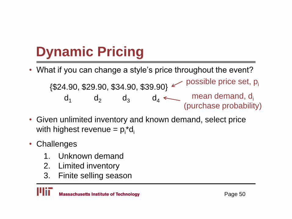
Dynamic Pricing
• What if you can change a style’s price throughout the event?
• Given unlimited inventory and known demand, select price
with highest revenue = pi*di
• Challenges
1. Unknown demand
2. Limited inventory
3. Finite selling season
Page 50
{$24.90, $29.90, $34.90, $39.90}
d1 d2 d3 d4
possible price set, pi
mean demand, di
(purchase probability)
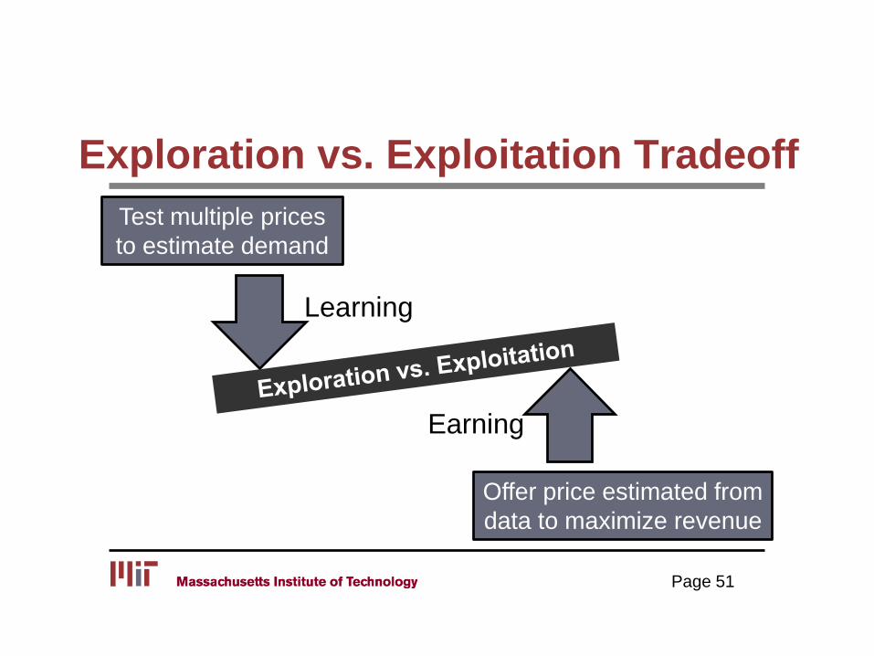
Exploration vs. Exploitation Tradeoff
Page 51
Learning
Earning
Test multiple prices
to estimate demand
Offer price estimated from
data to maximize revenue
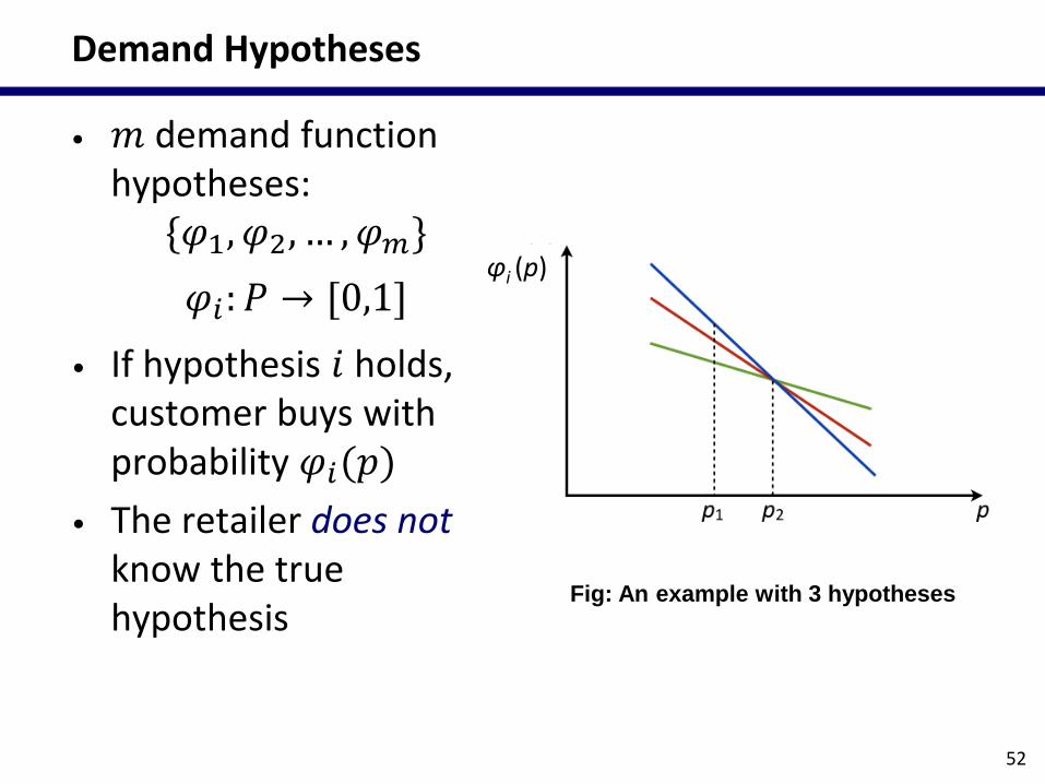
Demand Hypotheses
• 𝑚 demand function hypotheses:{𝜑1, 𝜑2, … , 𝜑𝑚}
𝜑𝑖: 𝑃 → [0,1]
• If hypothesis 𝑖 holds,customer buys with probability 𝜑𝑖(𝑝)
• The retailer does not know the true hypothesis
52
φi (p)
Fig: An example with 3 hypotheses
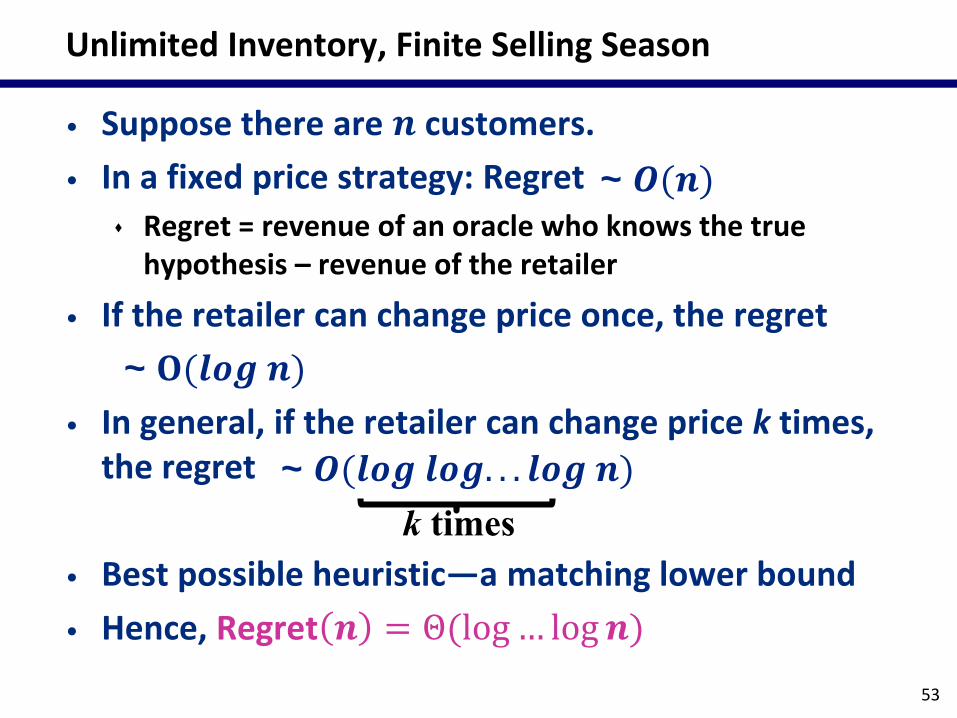
Unlimited Inventory, Finite Selling Season
• Suppose there are 𝒏 customers.
• In a fixed price strategy: Regret
Regret = revenue of an oracle who knows the true hypothesis – revenue of the retailer
• If the retailer can change price once, the regret
• In general, if the retailer can change price k times, the regret
• Best possible heuristic—a matching lower bound
• Hence, Regret 𝒏 = Θ(log… log 𝒏)
53
~ 𝑶(𝒏)
~ 𝐎(𝒍𝒐𝒈 𝒏)
~ 𝑶(𝒍𝒐𝒈 𝒍𝒐𝒈. . . 𝒍𝒐𝒈 𝒏)
k times
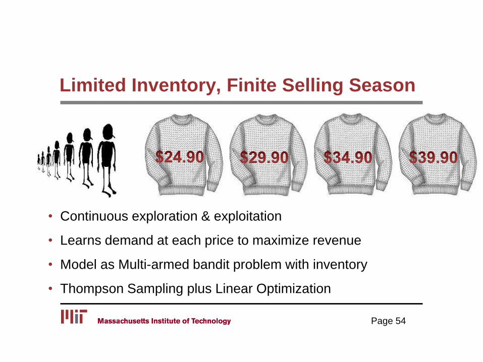
Limited Inventory, Finite Selling Season
• Continuous exploration & exploitation
• Learns demand at each price to maximize revenue
• Model as Multi-armed bandit problem with inventory
• Thompson Sampling plus Linear Optimization
Page 54
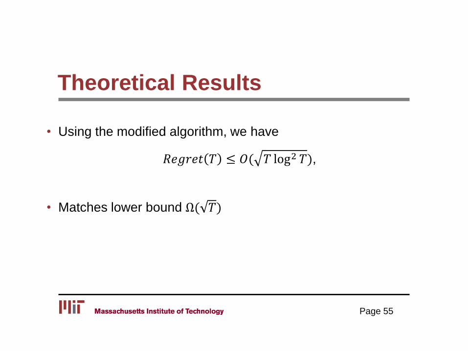
Theoretical Results
• Using the modified algorithm, we have
𝑅𝑒𝑔𝑟𝑒𝑡 𝑇 ≤ 𝑂( 𝑇 log2 𝑇),
• Matches lower bound Ω( 𝑇)
Page 55
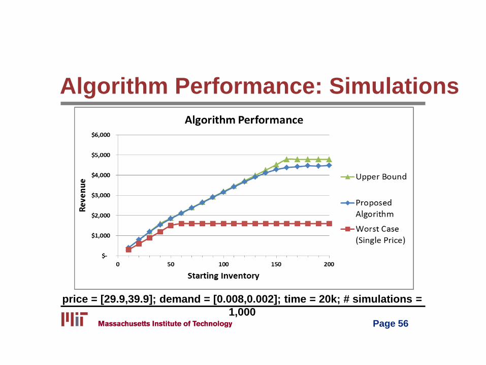
Algorithm Performance: Simulations
Page 56
price = [29.9,39.9]; demand = [0.008,0.002]; time = 20k; # simulations =
1,000

57
A Few Stories …
• From Theory to Practice
School Bus Routing in NYC
• From Practice to Theory
Flexibility at PepsiCo
• Merging Theory and Practice
Online Retailing
• Conclusions
Data Driven Models
57
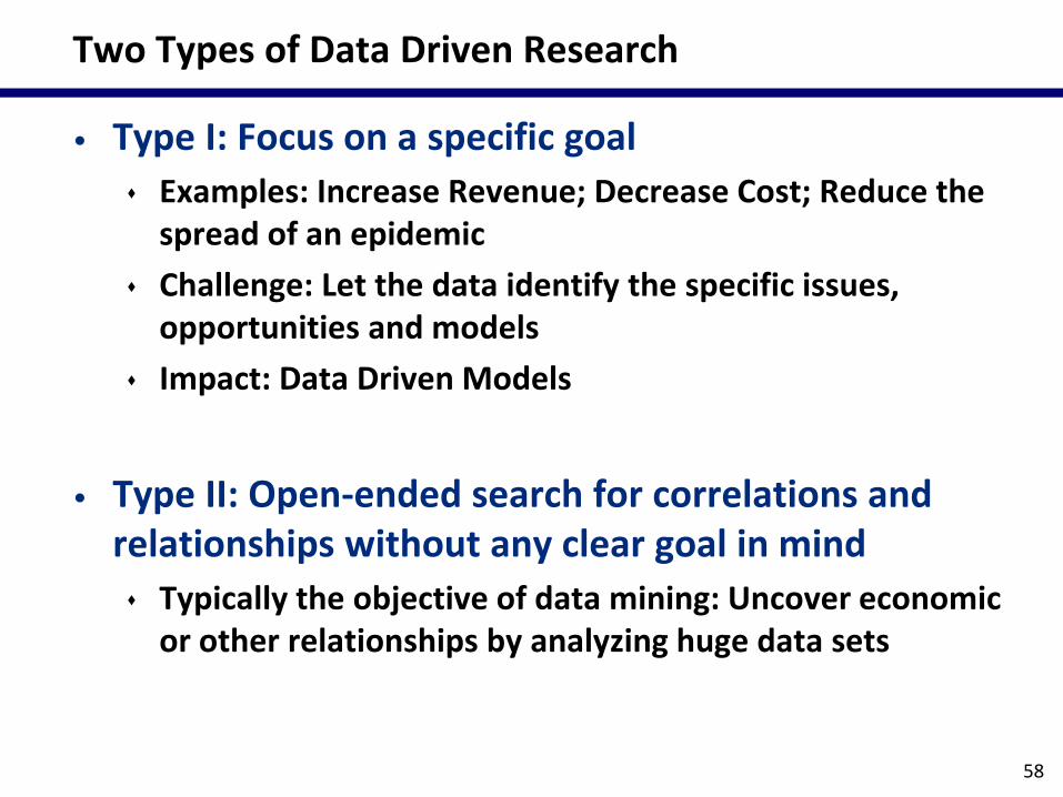
Two Types of Data Driven Research
• Type I: Focus on a specific goal
Examples: Increase Revenue; Decrease Cost; Reduce the spread of an epidemic
Challenge: Let the data identify the specific issues, opportunities and models
Impact: Data Driven Models
• Type II: Open-ended search for correlations and relationships without any clear goal in mind
Typically the objective of data mining: Uncover economic or other relationships by analyzing huge data sets
58
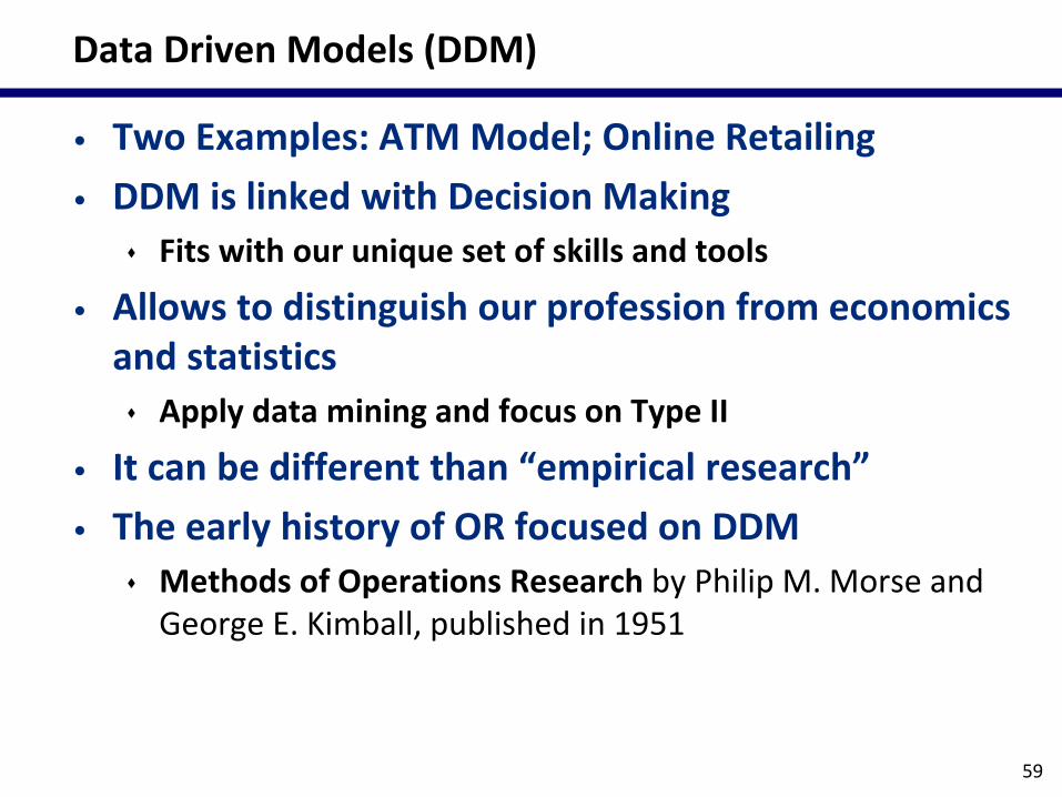
Data Driven Models (DDM)
• Two Examples: ATM Model; Online Retailing
• DDM is linked with Decision Making
Fits with our unique set of skills and tools
• Allows to distinguish our profession from economics and statistics
Apply data mining and focus on Type II
• It can be different than “empirical research”
• The early history of OR focused on DDM
Methods of Operations Research by Philip M. Morse and George E. Kimball, published in 1951
59
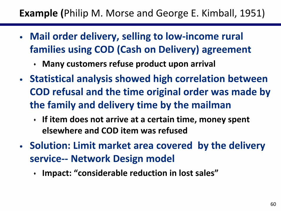
Example (Philip M. Morse and George E. Kimball, 1951)
• Mail order delivery, selling to low-income rural families using COD (Cash on Delivery) agreement
Many customers refuse product upon arrival
• Statistical analysis showed high correlation between COD refusal and the time original order was made by the family and delivery time by the mailman
If item does not arrive at a certain time, money spent elsewhere and COD item was refused
• Solution: Limit market area covered by the delivery service-- Network Design model
Impact: “considerable reduction in lost sales”
60
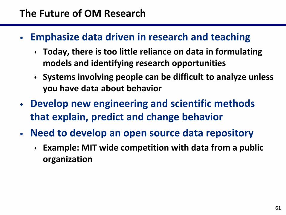
The Future of OM Research
• Emphasize data driven in research and teaching
Today, there is too little reliance on data in formulating models and identifying research opportunities
Systems involving people can be difficult to analyze unless you have data about behavior
• Develop new engineering and scientific methods that explain, predict and change behavior
• Need to develop an open source data repository
Example: MIT wide competition with data from a public organization
61
References…
• Simchi-Levi, D. (2014). OM Research: From Problem Driven to Data Driven Research. Manufacturing and Service Operations Management, Vol. 16, pp. 1-10.
• Johnson, K., Lee, B. H. A., and D. Simchi-Levi (2014). Analytics for an Online Retailer: Demand Forecasting and Price Optimization. 2014 INFORMS Revenue Management and Pricing Section Practice Award.
• Cheung W-C, Simchi-Levi D., Wang H. (2014). Dynamic Pricing and Demand Learning with Limited Price Experimentation. Submitted.
• Johnson, K., Simchi-Levi, D., and H. Wang (2014). Inventory-Constrained Demand Learning and Dynamic Pricing.
• Simchi-Levi, D., W. Schmidt and Y. Wei (2014), Managing Unpredictable Supply Chain Disruptions. HBR, January-February 2014, pp. 96-101. 2014 INFORMS Daniel H Wagner Prize for Excellence in Operations Research Practice
62