on instabilities in data assimilation algorithms · on instabilities in data assimilation...

School of Mathematical and Physical Sciences

Department of Mathematics and Statistics

Preprint MPS-2012-06

28 February 2012

On Instabilities in Data Assimilation Algorithms

by

Boris A. Marx and Roland W.E. Potthast

On Instabilities in Data Assimilation Algorithms

Boris A. Marx1 and Roland W.E. Potthast2,3

1 University of Gottingen, Germany, Graduiertenkolleg 1023 ”‘Identification in

Mathematical Models: Synergy of Stochastic and Numerical Methods”’2 German Meteorological Service - Deutscher Wetterdienst Research and

Development, Frankfurter Strasse 135, 63067 Offenbach, Germany3 University of Reading, Department of Mathematics, Whiteknights, PO Box 220,

Reading RG6 6AX, United Kingdom

Abstract. Data assimilation algorithms are a crucial part of operational systems in

numerical weather prediction, hydrology and climate science, but are also important for

dynamical reconstruction in medical applications and quality control for manufactoring

processes. Usually, a variety of diverse measurement data are employed to determine

the state of the atmosphere or to a wider system including land and oceans. Modern

data assimilation systems use more and more remote sensing data, in particular

radiances measured by satellites, radar data and integrated water vapor measurements

via GPS/GNSS signals. The inversion of some of these measurements are ill-posed in

the classical sense, i.e. the inverse of the operator H which maps the state onto the

data is unbounded. In this case, the use of such data can lead to significant instabilities

of data assimilation algorithms.

The goal of this work is to provide a rigorous mathematical analysis of the

instability of well-known data assimilation methods. Here, we will restrict our attention

to particular linear systems, in which the instability can be explicitly analyzed.

We investigate the three-dimensional variational assimilation and four-dimensional

variational assimilation. A theory for the instability is developed using the classical

theory of ill-posed problems in a Banach space framework. Further, we demonstrate

by numerical examples that instabilities can and will occur, including an example from

dynamic magnetic tomography.

1. Introduction

Data assimilation algorithms in combination with the reconstruction of quantities from

remote sensing data are important in many areas like numerical weather prediction

[War11], oceanic and hydrologic applications [PX09] as well as process tomography (for

example using magnetic tomography [KKP02], [HKP05], [HPWS05], [HP07], [HPW08],

[PW09], [Wan09]) and in cognitive neuroscience [PbG09].

Today, there is a variety of algorithms for data assimilation. There are classical

variational approaches (compare [LLD06], [LSK10]) known as three-dimensional

variational assimilation (3dVar) and four-dimensional variational assimilation (4dVar).

Many data assimilation schemes can be considered as special cases of statistical inversion

methods [Jaz70], [KS04], i.e. Bayesian estimation for the case of linear systems [RL00].

On Instabilities in Data Assimilation Algorithms 2

In the case of Gaussian errors and Gaussian background distributions for linear systems

Bayes’ formula leads to the well known Kalman Filter [Kal60].

Here, we study data assimilation algorithms as iterative or cycled schemes. Our

viewpoint is driven by the field of inverse problems, which rather than focusing on

stochastical properties of the fields under consideration, has placed strong emphasis on

the analysis of the ill-posedness of the reconstruction problem.

In fact, using remote sensing data we will find severe instabilities of these

algorithms. The origin of this instable behavior may either be due to the nonlinear

or chaotic systems dynamics as for examle presented in [CGTU08] or because of the

ill-posedness of the observation operator H. The second cause of instability is our key

concern in this work.

To provide a thorough analysis we investigate a dynamic (or cycled) Tikhonov

regularization scheme (compare also [Mar11]), which is a Tikhonov regularization with

a dynamic background which is updated by propagating the analysis of the previous

step to the next point in time where data are provided. We use the Hilbert spaces X, Y

and the discrete time-slices

t0 < t1 < t2 < ... < tk < . . . (1.1)

where we consider the system states xk ∈ X at time tk and the corresponding data

yk ∈ Y . They are given via the measurement operator H : X → Y by

yk = y(true)k + y(δ) = Hx

(true)k + y(δ), k ∈ N (1.2)

Let our measurement operator H be compact and linear and X be of infinite dimension.

Then, H cannot have a bounded inverse H−1 (c.f. [Kre99]). We need to employ

regularization which is implicitly carried out by classical variational data assimilation

schemes minimizing for example

J(x) := α||x− x(b)k ||

2 + ||yk −Hx(b)k ||

2 (1.3)

by the background term α||x− x(b)k ||2 given some state x

(b)k which is usually denoted as

the background at time tk. The minimizer x(a)k of (1.3) is called the analysis at time tk.

The propagation of the analysis x(a)k at time tk to the time tk+1 is carried out using the

model operator Mk+1|k : X → X by

x(b)k+1 = Mk+1|kx

(a)k . (1.4)

The equations (1.3) and (1.4) define the cycled Tikhonov regularization.

Our plan is as follows. In Section 2 we describe the setup of our systems. We

will base our arguments on the fact that the classical three-dimensional variational

assimilation (3dVar) and the fourdimensional variational assimilation (4dVar) for linear

systems can be rewritten as a cycled Tikhonov regularization when weighted norms are

introduced. So we can restrict our analysis to the case (1.3) - (1.4) and obtain results

which hold for key classical data assimilation methods.

In Section 3 we study the asymptotic behavior of x(a)k for k → ∞ when particular

model systems M are chosen for which we can explicitly carry out the asymptotic


analysis. These systems serve as key examples to prepare the investigation of more

complex nonlinear systems. In particular, we will study a constant system and spectrally

expanding or collapsing systems. We will show by functional analytic tools that for

compact observation operators H and data y(δ) /∈ H(X), the analysis will diverge for

k →∞.

Further, we provide a spectral view on the evolution in Section 3.2, for which

we provide explicit evolution formulas for the spectral coefficients of the analysis with

respect to the singular system of the observation operator. These formulas are also

provided for spectrally expanding or collapsing systems with a system dynamics which

is diagonal in the above singular system.

For the particular spectrally collapsing systems we show divergence of the relative

error when constant error terms are used in Section 3.3. For spectrally expanding

systems the relative error will tend to zero and convergence of the analysis towards the

dynamic true solution is shown.

The final Section 4 shows numerical examples for the asymptotic behavior. In

particular, we demonstrate the behavior for a spectral system where we have relatively

fast convergence of the spectral coefficients a(a)n,k of the analysis x

(a)k for small modes

and relatively slow convergence of the spectral analysis coefficients for large modes.

This leads to a particular behavior where we have a reduction of the analysis error

||x(a)k −x

(true)k || over some time, until the contribution of larger modes and the condition

y(δ) /∈ H(X) takes over and leads to a divergence of the analysis. We finally provide a

practical example from dynamic magnetic tomography which confirms this behavior.

2. System and Assimilation Setup

In this section we first introduce the model system setup which we will use as basis for

the subsequent instability study and then summarize the data assimilation algorithms

under consideration. We will also summarize the basic arguments why for linear model

dynamics both 3dVar and 4dVar can be considered as a cycled Tikhonov regularization

in a space with weighted norms, such that our analysis is valid for these assimilation

approaches.

2.1. Constant, spectrally expanding or collapsing systems.

Here, we will put a particular emphasis on situations where the phenomena can be

explicitly calculated. These are in particular

a) Constant systems. These are systems where Mk+1|k is the identity operator. Clearly,

constant dynamics is only a limiting case for very short time scales or slowly

changing situations. But the phenomena which appear here arising from ill-posed

observation operators will also be visible when the dynamics is no longer constant.

Also, the development of errors and iterates can be explicitly calculated.


b) Spectrally diagonal systems, i.e. systems for which the dynamics is given by

Mk+1|k = U−1DU (2.1)

with some orthonormal transformation U : X → X and a diagonal mapping D.

We call a mapping diagonal in an infinite dimensional space, when there is some

orthonormal system ϕn : n ∈ N such that

Dϕn = dnϕn, n ∈ N. (2.2)

c) Spectrally expanding systems. In the case where all dn satisfy

|dn| ≥ q > 1, n ∈ N, (2.3)

with some constant q we call the system expanding.

d) Spectrally collapsing systems. These are systems with a representation of type (2.1),

(2.2) for which

|dn| ≤ q < 1, n ∈ N (2.4)

with some constant q is satisfied.

We will also be interested in systems for which the columns of U are the singular

vectors of the measurement operator H, i.e. H∗Hϕn = µ2nϕn for n ∈ N. In this case, the

complete dynamics of the data assimilation system can be diagonalized by the singular

vectors of H.

2.2. Cycled Regularization

Tikhonov regularization is a well-known scheme to solve an ill-posed operator equation

of the type Hx = y by minimization of the cost functional

J(x) = ||Hx− y||2 + α||x||2. (2.5)

To solve such a data equation on successive points in time tk, we employ a modified

regularization term using the background

x(b)k+1 = Mk+1|kx

(a)k , k ∈ N (2.6)

which is calculated by propagating the analysis of the kth step by the model to

the time tk+1. An iterated Tikhonov scheme was analyzed in [Eng87] to find an

optimal regularization parameter for this iterated scheme. This is a special case of

our cycled scheme for a constant background. The cost functional for cycled Tikhonov

regularization is then

JT ik(x) = ||yk+1 −Hx||2 + α||x− x(b)k+1||

2 (2.7)

given measurements yk, k = 1, 2, 3, ... at time tk. The minimum of (2.7) is denoted as

x(a)k+1 (called the analysis). It is well-known that the normal equations for the quadratic

functional (2.7) lead to the update formula

x(a)k+1 = x

(b)k+1 +Rα

(yk+1 −Hx(b)

k+1

), k = 0, 1, 2, ... (2.8)


with

Rα = (αI +H∗H)−1H∗. (2.9)

starting from some initial state x(a)0 . The parameter α > 0 is denoted as regularization

parameter (compare [CK97] Theorem 4.14). We call (2.8) together with (2.6) the cycled

Tikhonov regularization.

2.3. Three-dimensional Variational Assimilation (3dVar).

Three-dimensional variational data assimilation (3dVar) is basically a cycled Tikhonov

scheme with weighted norms. For this section let us restrict our arguments to the n-

dimensional case where X = Rn with some n ∈ N and Y = Rm, m ∈ N. For some

symmetric positive definite matrix Γ we define the weighted scalar product

〈·, ·〉Γ := 〈· ,Γ·〉 , (2.10)

where 〈·, ·〉 denotes the standard L2 scalar product in Rn. Given a linear operator

H : X → Y , we denote the adjoint operator with respect to the standard scalar products

by H ′ and the adjoint with respect to the weighted scalar products by H∗.

Let B be the covariance matrix for the background system and R the covariance

matrix for the measurements. Then the cost function for the cycled 3dVar scheme

(compare [LLD06] Chapter 20) is given by

J3dV ar(x) = ||x− x(b)k+1||

2B−1 + ||yk+1 −Hx||2R−1 , (2.11)

which is minimized in each step by the analysis

x(a)k+1 = x

(b)k+1 +Kk+1

(yk −Hx(b)

k+1

)(2.12)

with the Kalman gain

Kk+1 = BH ′ (HBH ′ +R)−1. (2.13)

Theorem 2.1 For the common L2 scalar product 〈· , ·〉 and the weighted norms (2.10)

〈· , ·〉B :=⟨· , B−1·

⟩on X, 〈· , ·〉R :=

⟨· , R−1·

⟩on Y (2.14)

with self-adjoint, positive definite matrices B and R the Kalman gain (2.13) corresponds

to the Tikhonov projection (2.9) with the adjoint H∗ with respect to the weighted scalar

product 〈· , ·〉B, where the adjoint is given by

H∗ = BH ′R−1 (2.15)

Proof. The particular form (2.15) is obtained from

〈ϕ ,Hψ〉R =⟨ϕ ,R−1Hψ

⟩=⟨H ′R−1ϕ , ψ

⟩=⟨H ′R−1ϕ ,BB−1ψ

⟩=⟨BH ′R−1ϕ ,B−1ψ

⟩=⟨BH ′R−1ϕ , ψ

⟩B. (2.16)


We now study the relation between the Kalman gain (2.13) and the Tikhonov projection

(2.9). Using

H∗ (αI +HH∗) = (αI +H∗H)H∗ (2.17)

which leads to

(αI +H∗H)−1H∗ = H∗ (αI +HH∗)−1 (2.18)

we transform the Kalman gain (2.13) by

BH ′ (HBH ′ +R)−1

= BH ′R−1(HBH ′R−1 + I

)−1

= H∗ (HH∗ + I)−1

= (I +H∗H)−1H∗ (2.19)

which is the Tikhonov operator (2.9) for α = 1.

2.4. Four-dimensional Variational Assimilation (4dVar)

The 4dVar scheme minimizes a cost functional of the form

J4dV ar(x) := ||x− x0||2B−1 +K∑k=1

||yk −GMk|0x||2R−1k, (2.20)

where we now call the observation operator G for reasons which will be clear

immediately. For linear systems M it can be rewritten as the 3dVar scheme by redefining

the variables as follows. We define the vectorial observation space Y by

Y := Y × . . .× Y︸︷︷︸K times

(2.21)

and a vectorial observation operator

H :=

GM1|0...

GMK|0

(2.22)

and

y =

y1

...

yK

(2.23)

as well as the block diagonal covariance matrix for the measurements

R =

R1

. . .

RK

(2.24)

with block diagonal entries. A norm in Y is given by

||y||2R−1 = ||y1||2R−11

+ . . .+ ||yK ||2R−1K

(2.25)


with yj ∈ Y . Then we can write (2.20) as

J4dV ar(x) := ||x− x0||2B−1 + ||y −Hx||2R−1 , (2.26)

which corresponds to (2.11) for one iteration step. Thus, 4dVar for linear systems can be

written as a 3dVar algorithm and in a second step as a cycled Tikhonov regularization,

such that results for cycled Tikhonov regularization apply both 3dVar and 4dVar.

3. Instability of Variational Data Assimilation

The goal of this section is to carry out the stability analysis for cycled variational

assimilation algorithms with ill-posed observation operators, in particular for a cycled

Tikhonov regularization (which according to the above arguments then also hold for

3dVar and 4dVar). We will show that all cycled assimilation schemes can exhibit strong

instabilities when remote sensing operators are involved.

3.1. Cycled Tikhonov Regularization

We have shown that for linear models choosing appropriate norms the cycled 3dVar

or 4dVar can be written as a cycled Tikhonov regularization. Thus, without loss of

generality, we can restrict our attention to the update formula (2.8). We denote the

true system by x(true)k with true data y

(true)k = Hx

(true)k . The real measured data is

assumed to be of the form

yk = Hx(true)k + y

(δ)k , k ∈ N. (3.1)

Further, for simplicity we study a uniform time grid and use M for the system dynamics

from one time step to the next. In this case, we transform the update formula (2.8) into

x(a)k+1 = x

(b)k+1 +Rα

(yk+1 −Hx(b)

k+1

)= Mx

(a)k +RαH

(Mx

(true)k −Mx

(a)k

)+Rαy

(δ)k+1

= (I −RαH)Mx(a)k +RαHMx

(true)k +Rαy

(δ)k+1. (3.2)

Subtracting the true solution x(true)k+1 on both sides leads to

x(a)k+1 − x

(true)k+1 = (I −RαH)M

(x

(a)k − x

(true)k

)+Rαy

(δ)k+1 (3.3)

for k = 0, 1, 2, .... The formula (3.3) is a general formula which holds for a wide range

of systems. The case where we have the same type of error y(δ) = y(δ)k for all steps tk,

k = 1, 2, 3, ... constitutes a kind of worst case scenario, as we will see in more detail

below.

We denote the error between the analysis and true solution at time tk as ek. Then,

from (3.3) we obtain the error evolution

ek+1 = Λek + S, k = 0, 1, 2, ..., (3.4)

where we abbreviate

Λ := (I −RαH)M, S := Rαy(δ). (3.5)


The evolution of the error governed by the formula (3.4) can be carried out by an

induction proof as follows.

Lemma 3.1 Consider the evolution of some term ek ∈ X, k = 0, 1, 2, ..., in some

Banach space X given by (3.4) with initial value e0. Then, we obtain

ek = Λke0 +( k−1∑ξ=0

Λξ)S, k ∈ N. (3.6)

If (I − Λ) is invertible in X, then the formula can be transformed into

ek = Λk + (1− Λ)−1(1− Λk)S, k ∈ N. (3.7)

Proof. For k = 1 the formula (3.6) is clearly identical to the general update formula

(3.4). Assume that it is true for some k ∈ N, then we calculate

ek+1 = Λek + S

= Λ(

Λke0 +( k−1∑ξ=0

Λξ)S)

+ S

= Λk+1e0 +( k∑ξ=0

Λξ)S, (3.8)

which is the formula for k+1 and proves (3.6). If I−Λ is invertible, we use the telescopic

sum

(I − Λ)k−1∑ξ=0

Λξ = I − Λk (3.9)

and multiply by (I − Λ)−1 from the left to arrive at (3.7), which ends the proof.

As a consequence of the previous lemma we obtain the asymptotic behavior of the

error for cycled assimilation schemes. Here, we first study the case where M = I, i.e.

the model dynamics is the identity, as a basic reference situation. If things are instable

for this case, we cannot expect them to be stable in a more general setup. Here, we

have

Λ = I −RαH, I − Λ = RαH, S = Rαy(δ), (3.10)

leading to

Λ = I −RαH = I − (αI +H∗H)−1H∗H

= α(αI +H∗H)−1 = (I + α−1H∗H)−1. (3.11)

Clearly, the asymptotic behavior of ek for k →∞ is governed by the behavior of Λk for

k →∞. We carry out the convergence analysis in the following theorem.


Theorem 3.2 Assume that H : X → Y is a compact injective operator from a Hilbert

space X into a Hilbert space Y . Then we have the pointwise convergence(I + α−1H∗H

)−kϕ→ 0, k →∞ (3.12)

for every fixed element ϕ ∈ X.

Proof. To show the convergence (3.12) we use α = 1 to keep things readable, the

general case is carried out analogously. We have⟨(I +H∗H)ψ, (I +H∗H)ψ

⟩= ||ψ||2 + 2||Hψ||2 + ||H∗Hψ||2

> ||ψ||2 (3.13)

if Hψ 6= 0. If we use ψ = (I +H∗H)−1ϕ, we estimate

||(I +H∗H)−1ϕ|| < ||ϕ||. (3.14)

This observation can be generalized. We calculate⟨(I +H∗H)kψ, (I +H∗H)kψ

⟩= ||ψ||2 + 2k||Hψ||2 + Uk (3.15)

with some terms Uk for which we show later that they are positive or zero. As a

consequence we obtain

||(I +H∗H)−kϕ||2 + 2k||H(I +H∗H)−kϕ||2 < ||ϕ||2. (3.16)

Now, we know that λk := (I + H∗H)−kϕ is bounded in X. Assume that it is not

convergent towards zero. Then there is a weakly convergent subsequence (λkj)j∈N, which

tends weakly towards ψ ∈ X, ψ 6= 0. But now Hλkj → Hψ in X. From (3.16) we then

obtain Hψ = 0 and thus ψ = 0, which is a contradiction to our assumption and shows

that (3.12) must be satisfied.

Finally, we need to show that the terms Uk are positive. We use the binomial

formula to calculate⟨(I +H∗H)kψ, (I +H∗H)kψ

⟩=⟨ k∑ξ=0

(k

ξ

)(H∗H)ξψ,

k∑η=0

(k

η

)(H∗H)ηψ

⟩

=k∑ξ=0

k∑η=0

(k

ξ

)(k

η

)⟨(H∗H)ξψ, (H∗H)ηψ

⟩. (3.17)

Each scalar product in (3.17) can be seen to be positive by transforming them into terms

of the form ⟨(H∗H)lψ, (H∗H)lψ

⟩= ||(H∗H)lψ||2 (3.18)

with l = (ξ + η)/2 for ξ + η even or⟨(H∗H)l+1ψ, (H∗H)lψ

⟩= ||H(H∗H)lψ||2 (3.19)

with l = (ξ + η − 1)/2 for ξ + η odd, and the proof is complete.


For H injective we have shown the pointwise convergence Λke0 → 0 for k →∞ for

any e0 ∈ X. To fully study the behaviour of ek we further need to calculate the second

term in (3.6) or (3.7), respectively. We need to investigate

(I − Λ)−1S = (RαH)−1Rαy(δ). (3.20)

Under the condition that H∗H is invertible, we calculate

(RαH)−1Rα =(

(αI +H∗H)−1H∗H)−1

(αI +H∗H)−1H∗

= (H∗H)−1H∗, (3.21)

which is the Moore-Penrose pseudo inverse. Since H and H∗ are compact, in general

invertibility is not given, but we obtain invertibility of RαH on the subspace

Z := (αI +H∗H)−1H∗H(X) ⊂ Y.

We capture the phenomena in the following lemma.

Lemma 3.3 Assume that H and H∗ are injective. If y(δ) ∈ H(X), i.e. there is x(δ) ∈ Xsuch that y(δ) = Hx(δ), then with S = Rαy

(δ) we obtain( k−1∑ξ=0

Λξ)S → x(δ), k →∞. (3.22)

In the case where y(δ) 6∈ H(X), we have

||( k−1∑ξ=0

Λξ)S|| → ∞, k →∞. (3.23)

Proof. In the case y(δ) ∈ H(X) we have

(I − Λ)−1S = (RαH)−1RαHx(δ) = x(δ).

We use Theorem 3.2 for injective H∗H to derive

(I − Λk)(I − Λ)−1S = (I − Λk)x(δ) → x(δ). (3.24)

Using (3.9) and noting that the terms under consideration commute this yields( k−1∑ξ=0

Λξ)S → x(δ), (3.25)

which shows (3.22). To prove the second statement assume that

λk :=( k−1∑ξ=0

Λξ)S, k ∈ N, (3.26)

is bounded in X. Then, there is a weakly convergent subsequence and an element

ψ ∈ X such that λkj ψ for j → ∞. Since H is compact, it maps the weakly


convergent sequence into a strongly convergent sequence, i.e. Hλkj → Hψ. We further

have the convergence

(RαH)( kj−1∑

ξ=0

Λξ)S = (I − Λ)

( kj−1∑ξ=0

Λξ)S

= (I − Λkj)S

→ Rαy(δ), j →∞. (3.27)

and

(RαH)( kj−1∑

ξ=0

Λξ)S = RαHλkj

→ RαHψ, j →∞. (3.28)

Since Rα is boundedly invertible, from (3.27) and (3.28) we obtain the identity

Hψ = y(δ), i.e. y(δ) is in the images space H(X). This shows that under the condition

y(δ) 6∈ H(X) the sequence (λk)k∈N cannot be uniformly bounded and the proof is

complete.

Finally, we summarize our results and apply them to variational data assimilation

schemes as a corollary.

Corollary 3.4 (Instability of Assimilation Schemes) The cycled Tikhonov

regularization and thus also the data assimilation schemes 3dVar and 4dVar for a con-

stant model M and an injective compact observation operators are unstable when we

feed in data yk = Hx(true)k + y(δ), where y(δ) 6∈ R(H). If we have y(δ) = 0, we obtain con-

vergence towards the true solution x(true). If y(δ) = Hx(δ), we have convergence towards

x(true) + x(δ).

3.2. Spectral Cycled Tikhonov Scheme

The spectral approach (compare e.g. [CK97], Chapter 4.3) applied to the cycled data

assimilation provides further insight. We employ a singular system (ϕn, gn, µn) with an

orthonormal basis ϕn in X and an orthonormal basis gn in Y such that

Hϕn = µngn, H∗gn = µnϕn. (3.29)

For a state vector x ∈ X we denote the coefficients for the singular value decomposition

by an = 〈x, ϕn〉X . The coefficients of a true solution xtrue are defined by

xtrue =∞∑n=1

a(true)n ϕn. (3.30)

To include the temporal dimension we add the index k as in (2.6), i.e. we write

xk =∞∑n=0

an,kϕn,k k = 0, 1, . . . (3.31)


with coefficients an,k. The coefficients of the data vectors yk at time tk are defined by

yk =∞∑n=0

bn,kgn, k = 1, 2, . . . (3.32)

According to (3.29) an application of the operators H or H∗ corresponds to a spectral

multiplication by µn, n ∈ N and an application of H−1 corresponds to 1/µn, n ∈ N.

We use the notation

qn :=α

µ2n + α

, 1− qn =µ2n

µ2n + α

, n ∈ N. (3.33)

Then, in spectral terms we carry out the application of the following operators by

spectral multiplication in the sense of (3.29). For Rα = (I + H∗H)−1H∗ we spectrally

multiply byµn

α + µ2n

=(1− qn)

µn, n ∈ N.

In general, we have the spectral operations

H : an 7→ µnanRα : bn 7→ 1−qn

µnbn

I − Λ = RαH : an 7→ (1− qn)anΛ = I −RαH : an 7→ qnan

Λk = (I −RαH)k : an 7→ (qn)kan.

(3.34)

With this, the spectral version of the analysis step of the cycled Tikhonov scheme (2.8)

takes the form

a(a)n,k = a

(b)n,k +

1− qn,kµn

(bn − µna(b)

n,k

)= qn,ka

(b)n,k + (1− qn,k)

bnµn. (3.35)

For a constant model operator we have a(b)n,k = a

(a)n,k−1 for k = 1, 2, 3, .... We can then

formulate the spectral version of Lemma 3.1.

Lemma 3.5 For the cycled Tikhonov regularization scheme (3.35) with constant model

operator we have the spectral formula

an,k − a(true)n = qkn

(an,0 − a(true)

n

)+( k−1∑ξ=0

qξn

)1− qnµn

b(δ)n (3.36)

and

an,k − a(true)n = qkn

(an,0 − a(true)

n

)+ (1− qkn)

b(δ)n

µn(3.37)

Proof. We rewrite Lemma 3.1 using the spectral operations introduced above.

In spectral terms, the operator αk(αI + H∗H)−k is given by the multiplication by

αk(α+µ2n)−k. This now leads to an extended version and alternative proof for Theorem

3.2.


Theorem 3.6 Assume that H : X → Y is a compact operator from a Hilbert space X

into a Hilbert space Y . Then(I + α−1H∗H

)−kϕ→ 0, k →∞ (3.38)

for every fixed element ϕ ∈ X, ϕ ∈ N(H∗H)⊥. For ϕ ∈ N(H∗H) we obtain(I + α−1H∗H

)−kϕ = ϕ (3.39)

for all k ∈ N.

Proof. For ϕ ∈ N(H∗H)⊥ we represent the vector ϕ in the orthonormal system ϕnby

ϕ =∞∑n=1

anϕn. (3.40)

The application of (I + α−1H∗H)−1 to ϕn is given by multiplication with(1 +

µ2n

α

)−1

, n ∈ N. (3.41)

Since µ2n > 0, the term is bounded by 1 uniformly for all n ∈ N, which yields

||(I + α−1H∗H)−1|| ≤ 1.

Since µ2n → 0 for n→∞, we also know that for all ε > 0 we can find some n such that(

1 +µ2n

α

)−1

> (1− ε),

from which we obtain

||(I + α−1H∗H)−1|| = 1. (3.42)

The same argument applied to the k-th power of the term shows that we cannot obtain

norm convergence towards zero in (3.38). Clearly µ2n/α > 0 for every fixed n, thus we

obtain ∣∣∣(1 +1

αµ2n

)−k∣∣∣→ 0, k →∞ (3.43)

for fixed n ∈ N. To show (3.38) we now decompose ϕ into

ϕ =

n0∑n=1

βnϕn +∞∑

n=n0+1

βnϕn. (3.44)

Since ϕ ∈ X, we have∞∑

n=n0+1

|βn|2 → 0, n0 →∞. (3.45)

This yields ∣∣∣∣∣∣ (I + α−1H∗H)−k ∞∑

n=n0+1

βnϕn

∣∣∣∣∣∣2 ≤ ∞∑n=n0+1

|βn|2 → 0 (3.46)


for n0 →∞. Given ε > 0 we first choose n0 such that∑∞

n=n0+1 βnϕn is smaller than ε/2

in norm. Then, we choose k0 > 0 such thatn0∑n=1

∣∣∣(1 +1

αµ2n

)−kβn

∣∣∣2 < ε

2(3.47)

for k ≥ k0. This yields∣∣∣∣∣∣ (I + α−1H∗H)−k

ϕ∣∣∣∣∣∣2 ≤ ε, (3.48)

thus (3.38) is satisfied for k → ∞. To show (3.39) we employ the trivial identity

I = (I + α−1H∗H)− α−1H∗H to calculate

(I + α−1H∗H)−1ϕ = (I + α−1H∗H)−1

(I + α−1H∗H)− α−1H∗Hϕ

= ϕ− (I + α−1H∗H)−1α−1H∗Hϕ

= ϕ (3.49)

for ϕ ∈ N(H∗H), which ends the proof.

In particular, for the cycled Tikhonov scheme (2.8) with true data

bn = µna(true)n

we obtain

an,k = a(true)n − qkn

(a(true)n − an,0

)(3.50)

Since qkn → 0, k →∞ we obtain the spectral version of the convergence (3.22).

Corollary 3.7 For true data bn = µnan,true the cycled regularization scheme (3.35) is

given by (3.50) and the iterated coefficients converge toward the true solution

an,k → an,true, k →∞. (3.51)

We now consider noisy data, i.e. y = y(true) + y(δ) or the corresponding spectral

formula bn = µna(true)n +b

(δ)n . Applying Lemma 3.5 to measured data y with y(δ) ∈ H(X)

we obtain the following result.

Corollary 3.8 For data y = y(true) +y(δ) with y(δ) ∈ H(X), i.e. its spectral coefficient

b(δ)n is given by b

(δ)n = µna

(δ)n , the dynamic Tikhonov scheme (3.35) generates iterated

coefficients which converge toward some disturbed solution

an,k → a(true)n + a(δ)

n , k →∞. (3.52)

Thus for disturbed data the Tikhonov scheme converges but not to the true solution,

which is of course what we expect.

We now consider the case for y(δ) /∈ H(X) for which we will show the divergence

of the regularization scheme, now by spectral arguments. The following basic estimate

serves as a tool.


Lemma 3.9 Let a, b ∈ R, then we have

|a− b|2 ≥ |a|2

2− |b|2 (3.53)

Proof. We note

a2 = (a− b+ b)2 = (a− b)2 + 2(a− b)b+ b2 (3.54)

and from

0 ≤ (a− b− b)2 = (a− b)2 − 2(a− b)b+ b2

derive

2(a− b)b ≤ (a− b)2 + b2. (3.55)

Combining the two equations (3.54) and (3.55) we obtain (3.53). We are now prepared to show the basic divergence result.

Lemma 3.10 If yδ 6∈ Range(H) and yk = ytrue+yδ, then the dynamic Tikhonov scheme

(2.8) or (3.35), respectively, diverges, i.e.

||x(a)k || → ∞, k →∞. (3.56)

Proof. For yδ 6∈ H(X), due to Picard’s theorem (compare [CK97] Theorem 4.8),

we haveL∑n=0

∣∣∣∣ bnµn∣∣∣∣2 →∞, L→∞. (3.57)

We further have the following estimates for the coefficients: For every n ∈ N and

since 0 < qn < 1 we have∣∣qkn∣∣ ≤ 1,∣∣1− qkn∣∣ ≤ 1, ∀n, k ∈ N0. (3.58)

Using the representation (3.37), the bounds (3.58) and the general estimate from

Lemma 3.9 we obtain

||x(a)k ||

2 ≥L∑n=0

|an,k|2

=L∑n=0

∣∣∣∣qknan,0 + (1− qkn)a(true)n +

bnµn

(1− qkn)

∣∣∣∣2≥ 1

2

L∑n=0

∣∣∣∣ bnµn (1− qkn)

∣∣∣∣2 − L∑n=0

(∣∣qknan,0∣∣+∣∣(1− qkn)

∣∣ ∣∣a(true)n

∣∣)2

≥ 1

2

L∑n=0

∣∣∣∣ bnµn∣∣∣∣2 (1− qkn)2 − c (3.59)

for some constant c. For each fixed n we have (1 − qkn) → 0 for k → ∞. For some

constant C we first choose L such that the sum in (3.57) is larger than C + 2c. Then

for all sufficiently large k the sum in (3.59) is larger than C and therefore we have the

divergence (3.56).


3.3. Instability for spectrally expanding or collapsing systems

Finally, we will study the behaviour of the error of data assimilation algorithms with a

compact observation operator in the case of spectrally expanding or collapsing systems

as introduced in (2.1). We start with the spectral update formula (3.35) and use the

dynamics introduced in (2.2)

a(b)n,k+1 = dna

(a)n,k, k = 0, 1, 2, ... (3.60)

which is spectrally diagonal with respect to the singular system of the observation

operator H. In this case the coefficients show an exponential behaviour

a(true)n,k = dkna

(true)n,0 , k = 1, 2, 3, .... (3.61)

Then, the assimilation (3.35) with data yk = Hx(true)k + y

(δ)k , k = 1, 2, 3, ..., leads to the

update formula

a(a)n,k+1 = qndna

(a)n,k + (1− qn)a

(true)n,k+1 + (1− qn)

b(δ)n,k+1

µn. (3.62)

Note that the true solution is dynamical as well and we need to build this dynamics into

our induction formula to study the dynamical evolution of the analysis and the errors.

One key question is how the data error evolves. Here, we assume that

the measurements are remote sensing data which are independent of the system

development. This means that the data error is basically constant and does not change

over time, but the system expands or collapses. Then, the system development leads

to changes in the relationship between the size of the error and the size of the system,

such that the relative error changes significantly with time.

Lemma 3.11 Assume that we have data given by

yk = y(true)k + y(δ) = Hx

(true)k + y(δ). (3.63)

Then the updates (3.62) lead to an evolution of the analysis

a(a)n,k = qknd

knan,0 + (1− qkn)dkna

(true)n,0 +

( k−1∑ξ=0

qξndξn

)(1− qn)

b(δ)n

µn(3.64)

= qkndknan,0 + (1− qkn)a

(true)n,k + (1− dknqkn)

(1− qn)

(1− dnqn)

b(δ)n

µn. (3.65)

Proof. For k = 1 the formula (3.64) corresponds to (3.62). Assume it to be true

for some k ∈ N. Then we have

a(a)n,k+1 = qndna

(a)n,k + (1− qn)a

(true)n,k+1 + (1− qn)

b(δ)n

µn

= qndn

qknd

knan,0 + (1− qkn)dkna

(true)n,0 +

( k−1∑ξ=0

qξndξn

)(1− qn)

b(δ)n

µn

+ (1− qn)dk+1

n a(true)n,0 + (1− qn)

b(δ)n

µn


= qk+1n dk+1

n an,0 + (1− qk+1n )dk+1

n a(true)n,0 +

( k∑ξ=0

qξndξn

)(1− qn)

b(δ)n

µn,

which is the desired formula with k replaced by k + 1. Finally, (3.65) is obtained by

standard geometric series, and the proof is complete.

1) The Convergence Case. We can now investigate the asymptotic behavior, where

two main situations arise. We have convergent terms in (3.65) if the condition

|dnqn| =∣∣∣∣ αdnα + µ2

n

∣∣∣∣ < 1 (3.66)

is satisfied. The condition (3.66) can be rewritten as

|dn| < 1 +µ2n

α, n ∈ N. (3.67)

The spectral expansion coefficient dn needs to be bounded by (3.67) for the initial guess

term to decay. This reflects the general understanding that if the dynamical increase of

a mode is stronger than the decrease of its influence over time, the influence of the past

errors will increase in our current analysis.

The condition (3.66) is also needed for the third spectral term to converge.

Otherwise, the error which is coming in from y(δ) is increased in every step of the

time evolution.

(i) If the data error y(δ) is zero, then we obtain exponential convergence of the analysis

towards the dynamics of the true solution x(true)k , since qkn → 0 for k →∞.

(ii) If the measurement error in each step is given by y(δ) 6= 0, its spectral limit is

(1− qn)

(1− dnqn)

b(δ)n

µn=( µ2

n

(1− dn)α + µ2n

)b(δ)n

µn, n ∈ N, (3.68)

which leads to a constant regularized solution x(δ)α ∈ X in the case of strictly

spectrally collapsing dynamics, i.e. if |dn| ≤ ρ < 1 for all n ∈ N with some constant

ρ. In this case, where the true solution x(true)k is spectrally collapsing, i.e.∣∣∣x(true)

k

∣∣∣ ≤ ρk∣∣∣x(true)

0

∣∣∣ , k ∈ N, (3.69)

the error limit x(δ)α will gain more and more relative importance. The relative error

diverges.

(iii) If we have a spectrally expanding system where

|dnqn| ≤ ρ < 1, n ∈ N, (3.70)

we obtain

|dn| =ρ

|qn|→ ρ < 1, n→∞, (3.71)

which contradicts dn > 1, i.e. there cannot be spectrally expanding systems for

which (3.70) is satisfied.


Figure 1. The image displays the evolution of the analysis error for the cycled

Tikhonov regularization simulating the development of the analysis x(a)k for k → ∞

when y(δ) /∈ H(X). We observe that the analysis error first decays to some minimum

and then increases and becomes even larger than the error of a non-dynamic plain

Tikhonov regularization where we use a fixed background (dashed line).

2) Strong exponential system growth. If the expansion given by dn is too strong,

then it is not sufficient to look at the unscaled system, but again the relative error needs

to be studied. Here, we scale the growth by 1/dkn, i.e. we rescale everything to the size

of the true mode. Then

a(a)n,k

dkn= qknan,0 + (1− qkn)a

(true)n,0 +

(1

dkn− qkn

)(1− qn)

(1− dnqn)

b(δ)n

µn

→ a(true)n,0 , k →∞, (3.72)

i.e. in this case we have convergence of the scaled assimilation towards the true solution.

4. Numerical Examples

The task of this final part is to provide practical examples to demonstrate the behavior

described by the above theory. We first show a realization of the above spectral system

in Example 1, a second example is taken from dynamic magnetic tomography.

Example 1: Spectral System. Consider the application of 3dVar for data

assimilation where we assume a constant model system Mk+1|k = I and measured data


y = Hx(true) + y(δ) /∈ H(X). We have shown in Lemma 3.10 that in this case we have

||x(a)k || → ∞, k →∞. (4.1)

Further, from (3.37) we deduce that the spectral coefficient of the analysis error is

exponentially convergent towards

b(δ)n

µn, n ∈ N. (4.2)

The speed of this convergence is proportional to

qn =α

α + µ2n

, n ∈ N, (4.3)

i.e. it is depending on the particular mode. Since |µn| → 0 for n→∞ the convergence

is quick for small modes and decreases when n gets larger.

• When we have large initial error on small modes, this error will be quickly reduced

by the 3dVar cycling steps.

• Slowly we have the approximation of the higher error modes, such that there is

increasing error on the higher modes which tends to infinity for k →∞.

This can lead to a reduction of the error over some period of time [0, Tmin]. Then, when

the error of higher modes takes over, the error grows again in [Tmin,∞) with limit ∞at the right-hand side of the unbounded interval.

The results of the simulation are shown in Figure 1, where we see the behavior of

the total error of our system. The thick black line first shows a decay of the total error

until it reaches a minimum at Tmin. This corresponds to the part where the error in

the higher modes of of the error is small. In the second part we see that the total error

increases. The results confirm our theoretical considerations.

In the figure we also display a dotted line, where we employ Tikhonov regularization

for reconstruction without an update of the background, i.e. with a fixed background

chosen by the initial guess. So from the second step of the iteration we obtain a constant

reconstruction (due to our constant system and constant data we feed in). The cycled

3dVar starts with the same error, then improves and leads to a better reconstruction

for some time before it becomes distorted by the error y(δ) /∈ H(X). This means that

after some time T2 the error of the cycled scheme becomes larger than the error of the

plain non-dynamic Tikhonov regularization.

Example 2: Dynamic Magnetic Tomography. We provide a realistic

numerical example using the dynamic magnetic tomography problem as introduced

and analyzed in [Mar11]. Figure 2 shows the setup of fuel cell or fuel cell stack,

and corresponds to the domain Ω ∈ R3. In Ω we have the anisotropic conductivity

distribution x ∈ (L∞(Ω))3×3 and currents j ∈ (L2(Ω))3. Further we use the

measurement operator

W : (L∞(Ω))3×3 −→(L2(∂G)

)3, (4.4)

x 7−→ y.


Figure 2. Scheme representing the fuel cell domain with in- and outflowing Nodes,

conductivity (solid and dashed lines) and current density flow (red path) current

density distribution (colored boxes) and surrounding measurement surface (transparent

box surface) and measurement points.

with Ω ⊂ G, which maps the conductivity distribution x on the domain Ω onto the

magnetic field y on ∂G. We measure magnetic field data y on the boundary ∂G. Our

task is the dynamic reconstruction of the conductivity x.

From the literature we know that the classical problems consists of three major

parts, i.e. the model for the current density distribution give by a boundary value

problem as presented in [PK03]. The direct model given by the Biot-Savart operator

as e.g. also analyzed in [PK03] with several properties stated in [HKP05] and the

reconstruction step presented in [KKP02]. In [Mar11] the model was extended to use

it with data assimilation algorithms, i.e. we combine the boundary value formulation

with the Biot-Savart operator to state the direct magnetic tomography problem (4.4)

and solve it by using data assimilation algorithms from Section 2. For all details on the

dynamic magnetic tomography problem we refer to [Mar11].

Nonlinear Observation Operators. To treat nonlinear observation operators, we use

the Frechet derivative as follows. From [Mar11] we know that W is Frechet differentiable,

i.e. we have

W (x+ δx) = W (x) +W ′(x)δx+O(δx), δx ∈ X, (4.5)

with the Frechet derivative W ′(x) of W at the point x ∈ X. Then, at time tk+1 we need

to solve W (x+ δx) = y, which is approximated by

W (x) +W ′(x)δx = y ⇔ W ′(x)δx = y −W (x). (4.6)

This leads to the linearized version of the update, given by (2.12) with

Kk+1 = B(b)k+1(W ′(x

(b)k+1))∗

(W ′(x

(b)k+1)B

(b)k+1(W ′(x

(b)k+1))∗ +R

)−1

. (4.7)


100

101

102

103

2.16

2.18

2.2

2.22

2.24

2.26

2.28

2.3

2.32

2.34

2.36x 10

−3

time index k

erro

r

3dVar

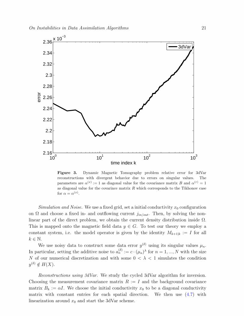
Figure 3. Dynamic Magnetic Tomography problem relative error for 3dVar

reconstructions with divergent behavior due to errors on singular values. The

parameters are α(x) := 1 as diagonal value for the covariance matrix B and α(r) = 1

as diagonal value for the covarince matrix R which corresponds to the Tikhonov case

for α = α(x).

Simulation and Noise. We use a fixed grid, set a initial conductivity x0 configuration

on Ω and choose a fixed in- and outflowing current jin/out. Then, by solving the non-

linear part of the direct problem, we obtain the current density distribution inside Ω.

This is mapped onto the magnetic field data y ∈ G. To test our theory we employ a

constant system, i.e. the model operator is given by the identity Mk+1|k := I for all

k ∈ N.

We use noisy data to construct some data error y(δ) using its singular values µn.

In particular, setting the additive noise to a(δ)n := c · (µn)λ for n = 1, ..., N with the size

N of our numerical discretization and with some 0 < λ < 1 simulates the condition

y(δ) /∈ H(X).

Reconstructions using 3dVar. We study the cycled 3dVar algorithm for inversion.

Choosing the measurement covariance matrix R := I and the background covariance

matrix Bk := αI. We choose the initial conductivity x0 to be a diagonal conductivity

matrix with constant entries for each spatial direction. We then use (4.7) with

linearization around x0 and start the 3dVar scheme.


Figure 3 shows the relative reconstruction error. We see that the error decreases

until it reaches a minmum after 11 steps. After that point the sum of the error according

to (3.57) takes over and the full system behaves as seen in (3.59). This confirms the

evolution given by Lemma 3.10 for a practically relevant example.

5. Summary

We have investigated the instability which can occur when measurements are assimilated

into a dynamical system evolution which are linked to the system state ϕ in an infinite

dimensional state space X by a compact measurement operator H. For simple systems

we have shown that cycling of standard data assimilation schemes can lead to severe

instabilities of the analysis, i.e. small measurement errors accumulate over time and can

lead to large analysis errors. We have worked out explicit spectral formulas which

show the instable behaviour. Further, numerical results in simple cases and from

dynamical magnetic tomography confirm the results. These results are interesting also

in seismology and earth sciences.

The systems investigated in this work can be seen as a simple model if the speed of

change in the dynamical system is small compared to the frequency of measurements.

But if even these quite stable systems can show severe instable behaviour, more general

systems are even more likely to show similar behaviour. Subsequent work has already

been carried out by Potthast, Moodey, Lawless and van Leeuwen [PMLvL], where

dynamical systems M of trace class are investigated. Note that the systems here, in

particular the constant system M = I, are not of trace class, but trace class systems

damp higher modes as it is usually carried out in global atmospheric models. For trace

class systems the authors show similar results, but also provide a stable assimilation

setup to control the analysis error over time. Further research in this direction is highly

interesting to learn more about possible instabilities of operational data assimilation

systems, which by causing large forecast error can have a significant impact on many

parts of society.

References

[CGTU08] Alberto Carrassi, Michael Ghil, Anna Trevisan, and Francesco Uboldi. Data assimilation

as a nonlinear dynamical systems problem: Stability and convergence of the prediction-

assimilation system. Chaos: An Interdisciplinary Journal of Nonlinear Science,

18(2):023112, 2008.

[CK97] David Colton and Rainer Kress. Inverse Acoustic and Electromagnetic Scattering Theory.

Springer, 2nd ed. edition, December 1997.

[Eng87] Heinz W. Engl. On the choice of the regularization parameter for iterated tikhonov

regularization of III-posed problems. Journal of Approximation Theory, 49(1):55–63,

January 1987.

[HKP05] Karl-Heinz Hauer, Lars Kuhn, and Roland Potthast. On uniqueness and non-uniqueness

for current reconstruction from magnetic fields. Inverse Problems, 21(3):955–967, 2005.

[HP07] Karl-Heinz Hauer and Roland Potthast. Magnetic tomography for fuel cells - current status

and problems. Journal of Physics: Conference Series, 73:012008 (17pp), 2007.


[HPW08] Karl-Heinz Hauer, Roland Potthast, and Martin Wannert. Algorithms for magnetic

tomography?on the role of a priori knowledge and constraints. Inverse Problems, 24,

2008.

[HPWS05] Karl-Heinz Hauer, Roland Potthast, Thorsten Wuster, and Detlef Stolten. Magnetotomog-

raphy – a new method for analysing fuel cell performance and quality. Journal of Power

Sources, 143(1-2):67–74, April 2005.

[Jaz70] Andrew H. Jazwinski. Stochastic processes and filtering theory. Academic Press, 1970.

[Kal60] RE Kalman. A new approach to linear filtering and prediction problems. Transactions of

the ASME - Journal of Basic Engineering, (82 (Series D)):35–45, 1960.

[KKP02] Rainer Kress, Lars Kuhn, and Roland Potthast. Reconstruction of a current distribution

from its magnetic field. Inverse Problems, 18(4):1127–1146, 2002.

[Kre99] Rainer Kress. Linear Integral Equations: v.82: Vol 82. Springer, 2nd ed. edition, April

1999.

[KS04] Jari Kaipio and E. Somersalo. Statistical and Computational Inverse Problems (Applied

Mathematical Sciences). Springer, 1 edition, December 2004.

[LLD06] John M. Lewis, S. Lakshmivarahan, and Sudarshan Dhall. Dynamic Data Assimilation: A

Least Squares Approach. Cambridge University Press, August 2006.

[LSK10] William Lahoz, Richard Swinbank, and Boris Khattatov. Data Assimilation: Making Sense

of Observations. Springer, June 2010.

[Mar11] Boris A. Marx. Dynamic Magnetic Tomography. Der Andere Verlag, May 2011.

[PbG09] Roland Potthast and Peter beim Graben. Inverse problems in neural field theory. SIAM

J. Appl. Dyn. Syst., 8(4):1405–1433, 2009.

[PK03] Roland Potthast and Lars Kuhn. On the convergence of the finite integration technique for

the anisotropic boundary value problem of magnetic tomography. Mathematical Methods

in the Applied Sciences, 26(9):739–757, 2003.

[PMLvL] Roland Potthast, Alexander J.F. Moodey, Amos S. Lawless, and Peter Jan van

Leeuwen. On error dynamics and instability in data assimilation. Preprint

http://www.reading.ac.uk/web/FILES/maths/preprint1205Lawless.pdf.

[PW09] Roland Potthast and Martin Wannert. Uniqueness of current reconstructions for magnetic

tomography in multilayer devices. SIAM Journal on Applied Mathematics, 70(2):563–

578, 2009.

[PX09] Seon K. Park and Liang Xu. Data Assimilation for Atmospheric, Oceanic and Hydrologic

Applications. Springer, 2009.

[RL00] Allan R. Robinson and Pierre F.J. Lermusiaux. Overview of data assimilation. Harvard

Reports in Physical/Interdisciplinary (Ocean Sciences); The Division of Engineering and

Applied Sciences Harvard University: Cambridge, Massachusetts, USA, 2000.

[Wan09] Martin Wannert. Stabile Algorithmen fur die Magnetotomographie an Brennstoffzellen.

PhD thesis, Universitat Gottingen, 2009.

[War11] Thomas Tomkins Warner. Numerical Weather and Climate Prediction. Cambridge

University Press, January 2011.

on instabilities in data assimilation algorithms · on instabilities in data assimilation...

Documents