on space and depth in resolution -...

ON SPACE AND DEPTH IN

RESOLUTION

Alexander Razborov

September 13, 2017

Abstract. We show that the total space in resolution, as well as inany other reasonable proof system, is equal (up to a polynomial and(log n)O(1) factors) to the minimum refutation depth. In particular, allthese variants of total space are equivalent in this sense. The sameconclusion holds for variable space as long as we penalize for exces-sively (that is, super-exponential) long proofs, which makes the ques-tion about equivalence of variable space and depth about the same asthe question of (non)-existence of “supercritical” tradeoffs between thevariable space and the proof length. We provide a partial negative an-swer to this question: for all s(n) ≤ n1/2 there exist CNF contradictionsτn that possess refutations with variable space s(n) but such that everyrefutation of τn with variable space o(s2) must have double exponential

length 22Ω(s). We also include a much weaker tradeoff result between

variable space and depth in the opposite range s(n) log n and showthat no supercritical tradeoff is possible in this range.

Keywords. Resolution proofs, supercritical tradeoff, variable and totalspace.

Subject classification. Mathematics Subject Classification (2010):Primary 03F20; Secondary 68Q17.

1. Introduction

The area of propositional proof complexity has seen a rapid devel-opment since its inception in the seminal paper Cook & Reckhow(1979). This success is in part due to being well-connected to anumber of other disciplines, and one of these connections that hasseen a particularly steady growth in recent years is the interplay

2 Alexander Razborov

between propositional proof complexity and practical SAT solving.As a matter of fact, SAT solvers that seem to completely dominatethe landscape at the moment (like those employing conflict-drivenclause learning) are inherently based on the resolution proof sys-tem dating back to the papers Blake (1937) and Robinson (1965).This somewhat explains the fact that resolution is by far the moststudied system in proof complexity, even if recent developments(see e.g. the survey Barak & Steurer (2014)) seem to be bringingthe system of sum-of-squares as a serious rival1.

Most of this study concentrated on natural complexity mea-sures of resolution proofs like size, width, depth or space andon their mutual relations; to facilitate further discussion, let usfix some notation (the reader not familiar with some or all ofthese is referred to Section 2 in which we give all necessary defini-tions). Namely, we let S(τn ` 0), ST (τn ` 0), w(τn ` 0), D(τn `0),CSpace(τn ` 0),TSpace(τn ` 0) and VSpace(τn ` 0) standfor the minimum possible size [tree-like size, width, depth, clausespace, total space2 and variable space, respectively]. w(τn) is thewidth of the contradiction τn itself.

Let us review some prominent relations between these mea-sures. The inequalities w(τn ` 0) ≤ D(τn ` 0) and logST (τn `0) ≤ D(τn ` 0) are trivial. Ben-Sasson & Wigderson (2001) con-joined them by proving that

(1.1) w(τn ` 0) ≤ logST (τn ` 0) + w(τn).

Even more importantly, in the same paper they established thecelebrated width-size relation

(1.2) w(τn ` 0) ≤ O(n · logS(τn ` 0))1/2 + w(τn)

1It should be remarked, however, that one of the most prominent SOSlower bound technique dating back to the paper Grigoriev (2001) is based onresolution width.

2 A word of warning about terminology: it is this measure that had beencalled “variable space” in Alekhnovich et al. (2002), and this usage of the termpersisted in the literature for a while, see e.g. Ben-Sasson (2009). But thenseveral good arguments were brought forward as to why it is more natural toreserve the term “variable space” for its connotative meaning, and we followthis revised terminology.

On Space and Depth in Resolution 3

that has steadily grown into a standard method of proving lowerbounds on the size of DAG resolution proofs.

In the space world, the obvious relations are CSpace(τn ` 0) ≤TSpace(τn ` 0) and VSpace(τn ` 0) ≤ TSpace(τn ` 0). CanCSpace(τn ` 0) and VSpace(τn ` 0) be meaningfully related toeach other?

In one direction this was ruled out by (Ben-Sasson 2009, The-orem 3.9): there are 3-CNF contradictions τn with CSpace(τn `0) ≤ O(1) and3 VSpace(τn ` 0) ≥ Ω(n/ log n).

Whether CSpace can be meaningfully bounded by VSpace isunknown. As will become clear soon, this question is extremelytightly connected to the content of our paper.

Let us mention several prominent and rather non-trivial resultsconnecting “sequential” measures (size, width, depth) and “config-urational”, space-oriented ones. Atserias & Dalmau (2008) provedthat

(1.3) w(τn ` 0) ≤ CSpace(τn ` 0) + w(τn);

a simplified version of their proof was presented by Filmus et al.(2015) and independently by Razborov (unpublished).

As we already observed, variable space can not be bounded interms of clause space, but Urquhart (2011) proved that it can bebounded by depth:

(1.4) VSpace(τn ` 0) ≤ D(τn ` 0).

In a recent paper Bonacina (2016), the following connectionbetween width and total space was established:

(1.5) w(τn ` 0) ≤ O(TSpace(τn ` 0))1/2 + w(τn)

that, similarly to (1.2), immediately opens up the possibility ofproving super-linear lower bounds on the total space in a system-atic way.

3Ironically (cf. Footnote 2), although this result was stated in Ben-Sasson(2009) for variable space, it was actually proved there only for what we callhere TSpace. However, the extension to VSpace is more or less straightforward,see e.g. Beck et al. (2013).


Finally, it should be mentioned that besides simulations therehave been proven quite a great deal of separation and tradeoffresults between these measures. They are way too numerous tobe meaningfully accounted for here, we refer the interested readerse.g. to the survey Nordstrom (2013).

Our contributions. We continue this line of research andprove both simulations and tradeoff results. In the former di-rection, perhaps the most catchy statement we can make is thatTSpace(τn ` 0) and D(τn ` 0) are equivalent, up to a polynomialand log n factors (see Figure 1.1 below for more refined statements).This is arguably the first example when two proof complexity mea-sures that are quite different in nature and have very different his-tory turn out not only to be tightly related to each other, butactually practically equivalent.

Now, in order to discuss these simulations and their ramifica-tions properly, we need to make up a few definitions.

For a configurational proof4 π, let VSpace∗(π)def= VSpace(π) ·

log2 |π|; a similar definition can be made for the total space andfor the clause space although we do not need the latter in ourpaper. Thus, we penalize refutations in a configurational formfor being excessively long; let us note that a similar logarithmicnormalization naturally pops up in many tradeoff results, see e.g.Ben-Sasson (2009). Then what we “actually” do is to show thatVSpace∗(τn ` 0) is polynomially related to depth; in particular, anysmall variable space proof can be unfolded into a shallow sequentialproof unless it is prohibitively long. Given this simulation, theequivalence for the total space is a simple artifact of the observationthat proofs with small total space can not be too long just becausethere are not that many possible different configurations. Morespecifically, we have the following picture in which, for the sakeof better readability, we have removed τn ` 0 elsewhere, replacedf ≤ O(g) with f g and taken the liberty to blend new results(that are essentially observations) with previously known ones, like(1.4), and trivial inequalities like D2 ≤ D3.

An immediate corollary is that TSpace, D,TSpace∗ and VSpace∗

4For definitions see Section 2 below.


VSpace TSpace D2≥ ≥

D VSpace∗ TSpace∗ D3

VSpace · (VSpace · log n+ 2VSpace) TSpace2 · log n

Figure 1.1: Simulations.

are all equivalent up to a polynomial and log n factors, and thesame applies for semantic versions of TSpace and TSpace∗.

The only difference between TSpace and VSpace is that in thefirst case we have a decent (that is, singly exponential) bound onthe overall number of configurations of small total space. Due tothe standard counting argument, this remains true for an arbitraryreasonable circuit class, and hence our equivalence uniformly gen-eralizes to the total space based on any one of them: polynomialcalculus with resolution, cutting planes etc. (Theorem 3.2). Allthese measures are essentially depth in disguise, and hence nΩ(1)

depth lower bounds automatically imply nΩ(1) lower bounds on thetotal space in all those models. For instance, for the total spacewe have

(1.6) Ω(D1/2) ≤ TSpace ≤ O(D2),

(the question how tight are these bounds will be addressed in theconcluding section 7).

In the rest of the paper, we study the relation of variable spaceitself to these equivalent measures; this question was (apparently)first asked by Urquhart Urquhart (2011). As follows from Figure1.1, this is equivalent to the following question: can the term 2VSpace

in the upper bound on VSpace∗ be really dominating or, in otherwords, can it be the case that the length of a configurational proofmust necessarily be super-exponential, as long as its variable spaceis relatively small? Note that this in particular would imply thatsuch a proof must mostly consist of totally non-constructive con-figurations so this situation may look a bit counterintuitive on the


first sight. However, precisely this kind of a behavior dubbed “su-percritical” tradeoffs was recently exhibited in Razborov (2016),and several other examples have been found in Berkholz & Nord-strom (2016a,b) and Razborov (2017).

Our most difficult result (Theorem 3.3) gives a moderate su-percritical tradeoff between variable space and proof length: forany s = s(n) ≤ n1/2, there are O(1)-CNF contradictions τn withVSpace(τn ` 0) ≤ s but such that every refutation π with sub-

quadratic variable space o(s2) must have length 22Ω(s). Improving

the space gap from sub-quadratic to super-polynomial would estab-lish a strong separation between the variable space and the depth,but that would probably require new techniques or at least quitea significant enhancement of ours. As a matter of fact, I am notready even to conjecture that a super-polynomial gap here exists,and perhaps VSpace after all is equivalent to all other measures onFigure 1.1.

The proof of Theorem 3.3 is highly modular and consists ofthree independent reductions; we review its overall structure atthe beginning of Section 6 where the statement is proven. Amongpreviously known ingredients we can mention r-surjective func-tions Alekhnovich & Razborov (2008), “hardness compression”Razborov (2016) and an extensive usage of the multi-valued logicin space-oriented models Alekhnovich et al. (2002). One new ideathat we would like to highlight is a “direct product result” Lemma6.9; results of this sort do not seem to be too frequent in the proofcomplexity. We use it to amplify our length lower bound for proofsof variable space 1 (that is, consisting of multi-valued literals) tothe same lower bound for proofs of larger variable space. This isprecisely this step that exponentially blows up the number of multi-valued variables and prevents us from extending this supercriticaltradeoff into a super-quadratic space range.

Finally, we look into the opposite range when VSpace(τn ` 0)is very small (say, a constant) and hence the term 2VSpace on Fig-ure 1.1 becomes negligible. In this regime, the syntactic measuresCSpace,TSpace become constant and, by (1.3), the same appliesto width. Razborov (2016) proved a supercritical tradeoff betweenwidth and depth, and Berkholz & Nordstrom (2016b) studied this


question for width vs. space, so it seems very natural to ask whatkind of tradeoffs might exist between space and depth. We proveboth positive and negative results in this direction. First, we ob-serve (Theorem 3.4) that the proof of the relation D ≤ VSpace∗ onFigure 1.1 can be generalized to showing that every (semantical)refutation of constant variable space gives rise, for an arbitraryparameter h, to a configurational refutation of variable space O(h)and depth h2 · nO(1/h); in particular, both space and depth canbe made poly-logarithmic, or depth can be brought down to n1/10

while space still remains constant. This rules out supercriticaltradeoffs in this context, at least as strong as those in Berkholz& Nordstrom (2016b); Razborov (2016). But we also show thatthis simulation is essentially the best possible: for the InductionPrinciple τn = x0, x0 → x1, . . . , xn−1 → xn, xn we show thatevery refutation π with variable space s must have depth nΩ(1/s)

(Theorem 3.5).

The structure of the paper corresponds to the above overview.In Section 2 we review all the necessary definitions, and in Section3 we state our main results. The next three sections are devotedto proofs: simulation results in Section 4, small space results inSection 5 and the supercritical tradeoff for large space5 in Section6. We conclude with a few remarks and open problems in Section7.

2. Notation and preliminaries

We let [n]def= 1, 2, . . . , n. |x| is the length of a word x, and xy

is the concatenation of two words. u is a prefix of v, denoted byu ≤ v if v = uw for another (possibly, empty) word w, and Λ isthe empty word.

For a Boolean function f , V ars(f) is the set of variables fessentially depends on. f |= g stands for semantical implicationand means that every assignment α satisfying f satisfies g as well.If τ and τ ′ are syntactic expressions like CNFs, the semanticalimplication τ |= τ ′ is understood in terms of the Boolean functions

5we defer our by far most difficult proof to the end


these expressions represent.A literal is either a Boolean variable x or its negation x; we will

sometimes use the uniform notation xεdef=

x if ε = 1

x if ε = 0. A clause

is a disjunction (possibly, empty) of literals in which no variableappears along with its negation. A generalized clause is either aclause or 1; the set of all generalized clauses makes a lattice in which∨ is the join operator. If C and D are clauses then C ≤ D in thislattice if and only if C |= D if and only if every literal appearingin C also appears in D. We will also sometimes say that C is asub-clause of D in this case. The empty clause will be denoted by0, and the set of variables occurring in a clause C, either positively

or negatively, will be denoted by V ars(C), let also V ars(1)def= ∅.

This is consistent with the general semantic definition. The width

of a clause C is defined as w(C)def= |V ars(C)|.

A CNF τ is a conjunction of clauses, often identified with theset of clauses it is comprised of. A CNF is a k-CNF if all clausesin it have width at most k. Unsatisfiable CNFs are traditionallycalled contradictions.

The resolution proof system operates with clauses, and it con-sists of the only resolution rule:

C ∨ x D ∨ xC ∨D

.

Two major topologies used for representing resolution proofs aresequential (Hilbert-style) and configurational (or space-oriented).In order to distinguish between them, we use upper-case letters Πfor the former and lower-case π for the latter.

A (sequential) resolution proof Π is a DAG with a unique targetnode in which all nodes are labeled by clauses, every non-sourcenode v has fan-in 2, and the clause assigned to v can be inferredfrom clauses sitting at its predecessors via a single application ofthe resolution rule. A resolution proof of a clause C from a CNFτ is a resolution proof Π in which all source nodes are labeled byclauses from τ , and the target node is labeled by a sub-clause6 of

6This is a technicality that is necessary since we did not explicitly includethe weakening rule.


C. A refutation of a contradiction τ is a proof of 0 from it. Thesize S(Π) of a sequential proof is the number of nodes, its depthD(Π) is the length of the longest path in the underlying DAG, andits width w(Π) is the maximal possible width w(C) of a clause Cappearing in it. For a contradiction τ , we let S(τ ` 0), D(τ ` 0)and w(τ ` 0) denote the minimal possible value of S(Π), D(Π)and w(Π), respectively, taken over all sequential refutations Π ofτ .

The configurational (or space-oriented) form of propositionalproofs was introduced in Alekhnovich et al. (2002); Esteban &Toran (2001). A configuration C is a set of generalized clauses thatcan be viewed as a CNF. A configurational proof π from a CNFformula τ is a sequence of configurations (C0, . . . ,CT ) in whichC0 = ∅ and every Ct (t ∈ [T ]) is obtained from Ct−1 by one of thefollowing rules:

Axiom Download. Ct = Ct−1 ∪ A, where A ∈ τ ;

Inference. Ct = Ct−1 ∪ C for some C 6∈ Ct−1 inferrable by asingle application of the resolution rule from the clauses inCt−1.

Erasure. Ct ⊆ Ct−1.

π is a (configurational) refutation of τ if 0 ∈ CT . T is the lengthof π, denoted by |π|.

The clause space of a configuration C is |C|, its total spaceTSpace(C) is

∑C∈Cw(C), and its variable space VSpace(C) is∣∣⋃

C∈C V ars(C)∣∣. The clause [total] space CSpace(π) [TSpace(π),

respectively] of a configurational proof π is the maximal clause[total, respectively] space of all its configurations, and if τ is acontradiction, then CSpace(τ ` 0) [TSpace(τ ` 0)] is the minimumvalue of CSpace(π) [TSpace(π), respectively], where the minimumis taken over all configurational refutations π of τ .

Variable space VSpace(τ ` 0) can be of course defined analo-gously, but since this measure is inherently semantical, we preferto stress this fact by giving a separate, and more robust, definitionbelow.


Definition 2.1. Let τ be an arbitrary set of Boolean constraints.For a set V of variables, we let

τ [V ]def=∧C | C ∈ τ ∧ V ars(C) ⊆ V .

A semantical proof π from τ is a sequence of Boolean functions(f0, . . . , f1, . . . , fT ) such that f0 ≡ 1 and for every t ∈ T ,

(2.2) ft−1 ∧ τ [V ars(ft−1) ∪ V ars(ft)] |= ft.

T is again the length of π, denoted by |π|, and π is a semanti-

cal refutation if fT ≡ 0. VSpace(π)def= max0≤t≤T |V ars(ft)| and

VSpace(τ ` 0) is the minimum value of VSpace(π) taken over allsemantical refutations π of τ .

In this definition we have combined all three rules (AxiomDownload, Inference and Erasure) into one. Every configu-rational proof turns into a semantical proof of (at most) the samevariable space if we replace all configurations in it by the Booleanfunctions they represent. Hence VSpace(τ ` 0) never exceeds itssyntactical variant, and in the other direction (when τ is actuallya CNF), they may differ by at most a factor of 2 simply by ex-panding all semantical refutations (2.2) into brute-force resolutionderivations never leaving the set of variables V ars(ft−1)∪V ars(ft).

This purely semantical model also provides a handy uniformway to talk about semantical analogues of more sophisticated spacecomplexity measures. Namely, let C be a circuit class equippedwith a complexity measure µ(C) (C ∈ C). Then µ gives rise to thecomplexity measure on Boolean functions in a standard way: µC(f)is the minimum value of µC taken over all circuits C ∈ C computing

f . For a semantical refutation π, let us define µC-Space(π)def=

max0≤t≤T µC(ft) and then µC-Space as usual. This definition mayseem overly broad at the first glance, but we will see in Theorem3.2 that under very mild conditions on the circuit class C, thismeasure will also turn out to be equivalent to depth.

Examples. Semantical analogues of clause and total spacestudied in the literature before correspond to the case when C con-sists of all CNFs, and the measures µC are the number of clauses


or overall size, respectively. Semantical analogues of, say, cuttingplanes space or PCR space are also straightforward in this lan-guage.

Finally, we need several mixed, “amortized” measures that pe-nalize configurational proofs for being unreasonably long. We let

TSpace∗(π)def= TSpace(π) · log2 |π|,

VSpace∗(π)def= VSpace(π) · log2 |π|,

µC-Space∗(π)

def= µC-Space(π) · log2 |π|,

and then we define TSpace∗(τ ` 0) VSpace∗(τ ` 0) and µC-Space∗(τ `

0) as usual (CSpace∗(τ ` 0) can be also defined likewise, but we donot need it in this paper).

Definition 2.3. For a configurational proof π = (C0,C1, . . . ,CT ),define integer valued depth functions Dt on Ct by induction on t.Since C0 is empty, there is nothing to define. Let t > 0, assumethat C ∈ Ct and that Dt−1 is already defined. If C ∈ Ct−1, we

simply let Dt(C)def= Dt−1(C). If A ∈ τ in the Axiom Download

Rule then Dt(A)def= 0. If C is obtained from C ′, C ′′ ∈ Ct−1 via

the resolution rule, we let

Dt(C)def= max(Dt−1(C ′), Dt−1(C ′′)) + 1.

Finally, the depth D(π) of a configurational refutation π is definedas DT (0).

Let us remark that Boolean restrictions naturally act on con-figurational refutations, and that under this action neither space(any flavor) nor depth may increase.

3. Main results

As all our results were discussed at length in the introduction, herethey are listed more or less matter-of-factly.

In order to improve readability, in our first theorem 3.1 we omitthe argument τn ` 0 throughout (τn is an arbitrary contradictionin n variables), and also we write f g for f ≤ O(g). Also, we


include here both previously known results and trivial simulations;for explicit tags see the proof given in the next section. Arguably,the only non-trivial new part in the whole table is the simulationD VSpace∗.

Theorem 3.1. For the proof-complexity measuresD,TSpace,VSpace,TSpace∗,VSpace∗ introduced in Section 2 wehave the following simulations:

VSpace TSpace D2

≥ ≥

D VSpace∗ TSpace∗ D3

VSpace · (VSpace · log n+ 2VSpace) TSpace2 · log n.

Theorem 3.2. Let C be any circuit class that includes CNFs,and let µC be any complexity measure on C that is intermediatebetween the number of input variables and the circuit size of C ∈ C.Then µC-Space(τn ` 0) is equivalent, up to a polynomial and log nfactors to D(τn ` 0) (and hence to all other measures in Theorem3.1 except, possibly, VSpace).

Theorem 3.3. Let s = s(n) ≤ n1/2 be an arbitrary parameter.Then there exists a CNF τn with VSpace(τn ` 0) ≤ s but such thatfor any semantical refutation π of τn with VSpace(π) ≤ o(s2) wehave |π| ≥ exp(exp(Ω(s))).

The next result is a variation on the simulation D VSpace∗

in Theorem 3.1.

Theorem 3.4. Assume that a contradiction τ possesses a seman-tical refutation π with VSpace(π) = s and |π| = S, and let h ≥ 1be an arbitrary parameter. Then τ also has a configurational refu-tation π′ with VSpace(π′) ≤ O(sh) and D(π′) ≤ O

(sh2 · S1/h

).


Theorem 3.5. Let τn = x0, x0 ∨ x1, x1 ∨ x2, . . . , xn−1 ∨ xn, xn.Then for every configurational refutation π from τn we have thebound

D(π) ≥ Ω(n1/VSpace(π)

).

4. Proofs of simulations

In this short section we prove Theorems 3.1 and 3.2.

Proof of 3.1. The square

VSpace ≤ TSpace

≥

VSpace∗ ≤ TSpace∗

is obvious.

Variable space is upper bounded by depth.VSpace(τ ` 0) ≤ D(τ ` 0) is (Urquhart 2011, Theorem 6.1(1)).

Total space is upper bounded by depth squared.This is a minor variation on (Esteban & Toran 2001, Theo-

rem 2.1). Indeed, let Π be a refutation of a contradiction τ withD(Π) = d, then w.l.o.g. we can assume that Π is in a tree-likeform. Also, w(Π) ≤ d since every variable in the clause at anode v must be resolved on the path from v to the target (root)node. We now consider the standard pebbling of the underlyingtree with (d + 1) pebbles and the resulting configuration refuta-tion π = (C0,C1, . . . ,CT ), as in Esteban & Toran (2001). As areminder, we can assume w.l.o.g. that Π is a complete binary treeof height d, identify its nodes with binary words α of length ≤ din such a way that α0 and α1 are the two children of α, and let

Cα be the corresponding clauses so thatCα0 Cα1

Cαis an in-

stance of the resolution rule. Ct then consists of all those Cα forwhich α1d−|α| ≤ t, where the left-hand side is interpreted as aninteger in the binary notation, and that are maximal with thisproperty (i.e., either α = Λ or α = β0 with β1d+1−|α| > t). It


can be readily checked that Ct+1 is obtained from Ct by a sin-gle Axiom Download rule, followed by at most d Influence-Erasure pairs, and that |Ct| ≤ d + 1. Since also every clausein π has width ≤ d (due to the above remark) and T ≤ 2d+1,both claims TSpace(τ ` 0) ≤ D(τ ` 0)(D(τ ` 0) + 1) andTSpace∗(τ ` 0) ≤ D(τ ` 0)(D(τ ` 0) + 1)2 now follow.

“Amortized” space is upper bounded by ordinary space.

We need to prove that

TSpace∗(τn ` 0) ≤ 2 log2(2n+ 1)TSpace(τn ` 0)2

and

VSpace∗(τn ` 0)

≤ VSpace(τn ` 0)(VSpace(τn ` 0) log2 n+ 2VSpace(τn`0)

).

Both bounds follow from the observation that a configurationalrefutation (be it syntactic or semantic) can w.l.o.g. be assumed notto contain repeated configurations. Now, we estimate the overallnumber of configurations C = C1, . . . , Ck with total space ≤ sby encoding them as a string C1#C2# . . .#Ck# . . . of length 2sin which the clauses Ci are written down simply as sequences ofliterals. We conclude that the overall number of different configu-rations C of total space ≤ s is bounded by (2n+1)2s, which gives usthe first statement. Likewise, the overall number of Boolean func-tions f with |V ars(f)| ≤ s is upper bounded by

(ns

)22s ≤ ns22s ,

and this gives us the second statement.

Depth is upper bounded by amortized variable space.

This is by standard binary search. Let π = (f0, f1, . . . , fT )be a semantical refutation from τ minimizing VSpace∗(π), and let

sdef= VSpace(π). We prove by induction on d that for every 0 ≤ a <

b ≤ T with b− a ≤ 2d and for any clause C in the straightforwardCNF expansion of the implication fa → fb (that is to say, for everyclause C with V ars(C) = V ars(fa)∪V ars(fb) and (fa → fb) |= C)we have D(τ ` C) ≤ 2s(d+ 1).

Induction base d = 0, b = a+ 1.


We have fa ∧ τ [V ars(fa) ∪ V ars(fa+1)] |= fa+1, hence

τ [V ars(fa) ∪ V ars(fa+1)] |= (fa → fa+1) |= C.

Since |V ars(fa) ∪ V ars(fa+1)| ≤ 2s, we can realize the latter se-mantical refutation by a resolution refutation of depth ≤ 2s.

Inductive step: d ≥ 1, 2 ≤ b− a ≤ 2d.Pick c with a < c < b such that c − a, b − c ≤ 2d−1. Then C

has an obvious resolution proof of depth |V ars(fc) \ (V ars(fa) ∪V ars(fb))| ≤ s from clauses C appearing in the CNF expansions

of fa → fc and fc → fb. Since D(τ ` C) ≤ (d − 1)s for any suchclause by the inductive assumption, the inductive step follows.

In particular, setting d = log2 T , a = 0, b = T, C = 0, weconclude that D(τ ` 0) ≤ (2s) log2 T ≤ 2VSpace∗(π).

Proof of 3.2. Take the configurational refutation (C0,C1, . . . ,CT )of τ with total space TSpace(τ ` 0) and convert it to the semanticalform (f0, f1, . . . , fT ). Since C contains all CNFs and µC does notexceed the circuit size, we conclude that µC(ft) ≤ O(TSpace(Ct))and hence µC-Space(τ ` 0) ≤ O(TSpace(τ ` 0)). On the otherhand, since µC is bounded from below by the number of essen-tial variables, for every semantical proof π we have VSpace(π) ≤s

def= µC-Space(π). If π in addition is minimal, then the length

is bounded by the overall number of circuits C in C that satisfyµC(C) ≤ s and hence, using again the condition on µC, have size≤ s. Since the number of circuits of size s is bounded (to be on thesafe side) by nO(s), the bound VSpace∗(π) ≤ O(s2 log n) follows. AsVSpace∗ and TSpace are equivalent up to a polynomial and log nfactors, the same holds for µC-Space.

5. Very small space

In this section we prove Theorems 3.4 and 3.5 (as we noted inthe introduction, we defer our most challenging proof to the nextsection).

Proof of 3.4. As we already remarked, this is a variation onthe proof of Theorem 3.1 (the D(τ ` 0) ≤ 2VSpace∗(τ ` 0) part),


except that instead of binary search we now do T -ary search for asuitable T . But this time our goal is to come up with a configura-tional refutation rather than a tree-like one. Hence, an inductivedescription would be somewhat awkward, and we frame the argu-ment as a direct construction instead.

Let π = (f0, f1, . . . , fS) be a semantical refutation from τ thathas variable space ≤ s. Assume w.l.o.g. that S is of the form(T + 1)h − 1 for an integer T , and for t ∈ [0..S], let (th−1, . . . , t0)be its (T + 1)-ary representation, that is t =

∑h−1d=0 td(T + 1)d. For

t > 0, let ord(t) be the minimal d for which td 6= 0 (that is, themaximal d for which (T + 1)d|t). Let t(k) be the truncation of t

by taking k most significant bits: t(k) def=∑h−1

d=h−k td(T + 1)d. In

particular, t(0) = 0 and t(h) = t. Let

ftdef= (f0 → ft(1)) ∧ (ft(1) → ft(2)) ∧ . . . ∧ (ft(h−1) → ft).

Clearly, |V ars(ft)| ≤ O(hs).

Let us now take a look at ft+1. Denoting kdef= h−ord(t+1), let

us note that (t+1)(k) = (t+1)(k+1) = . . . = (t+1)(h−1) = t+1 sincein all those cases we truncate zeros only. Hence we can remove fromft+1 all trivial terms f(t+1)(k) → f(t+1)(k+1) , . . . , f(t+1)(h−1) → ft+1

and write it down simply as

ft+1 ≡ (f0 → ft(1)) ∧ (ft(1) → ft(2)) ∧ . . .∧ (ft(k−2) → ft(k−1)) ∧ (ft(k−1) → ft+1).

Hence ft ∧ (ft → ft+1) |= ft+1 and (f0, f1, . . . , fs) is also a seman-tical refutation from τ of the desired variable space O(hs).

We convert it to a configurational resolution refutation as fol-lows. First, for t ≤ t′ denote by C(t, t′) the straightforward CNF-

expansion of ft → ft′ . Next, let Ctdef= C(0, t(1)) ∪ C(t(1), t(2)) ∪ . . . ∪

C(t(h−1), t); this is our chosen CNF representation of the Boolean

function ft. Now the conversion is natural: to get from Ct to Ct+1,we first download all axioms in τ [V ars(ft)∪V ars(ft+1)], then writedown the brute-force inference

C(ft(k−1) , ft(k)), . . . , C(ft(h−1) , ft), τ [V ars(ft) ∪ V ars(ft+1)](5.1)

` C(ft(k−1) , ft+1),


and, finally, erase all clauses in the left-hand side. It remains tobound the depth of this refutation (recall Definition 2.3).

Every individual step (5.1) has depth O(hs) as this is how manyvariables it involves. To get a bound on the depth of the tree formedby the inferences (5.1), we not that for every C(fa, fb) in the left-hand side either ord(b) < ord(t + 1)(= h − k): this happens forall configurations but C(ft(k−1) , ft(k)), or ord(b) = ord(t + 1) andb < t + 1 (a = t(k−1), b = t(k), th−k 6= 0), or it is trivial and canbe removed (a = t(k−1), b = t(k), th−k = 0). Hence the depth ofthe proof tree defined by the inferences (5.1) is O(hT ), and therequired overall bound O(h2sT ) on depth follows.

Proof of 3.5. Fix a configurational refutation π = (C0,C1, . . . ,CT )from the Induction Principle τn that has variable space s. Let usbegin with a few generic remarks.

First, we can assume w.l.o.g. that for every 0 ≤ t ≤ T − 1, Ct

does not contain the empty clause 0.Next, let us call a clause Bi-Horn if it contains at most one

occurrence of a positive literal and at most one occurrence of anegative literal. Since the set of bi-Horn clauses is closed underthe Resolution rule, and all axioms in τn are bi-Horn, all clausesappearing in our refutation must be also bi-Horn. In other words,for every t < T , Ct must entirely consist of literals and implicationsof the form xi → xj (i 6= j).

Next, for t ≤ T − 1 we can remove from Ct all clauses C withDt(C) ≥ D(π) and still get a configurational refutation (this reduc-tion corresponds to removing non-essential clauses in Ben-Sasson(2009)). Hence, we can assume that

(5.2) Dt(C) ≤ D(π)− 1, t ≤ T − 1, C ∈ Ct.

Let us now return to the proof of Theorem 3.5. The config-uration CT−1 must contain both literals xi, xi of some variable i.Let r be the maximal index for which xr, viewed as a one-variableclause, appears anywhere in π, and let ` be the minimal index forwhich the clause x` occurs there. Note that ` ≤ i ≤ r, and henceV ars(CT−1) has a non-empty intersection with both x0, . . . , xrand x`, x`+1, . . . , xn.


Choose a such that

V ars(Ca)∩x0, x1, . . . , xr 6= ∅ ∧ V ars(Ca)∩x`, x`+1, . . . , xn 6= ∅

while for Ca−1 one of these properties is violated. By symmetry,we can assume w.lo.g. that V ars(Ca−1) ∩ x0, . . . , xr = ∅.

Let us now apply to π the restriction ρ+ : x0 → 1, x1 →1, . . . , x` → 1. It transforms τn to τn−`−1, and since x` appearssomewhere in the refutation (and is killed by ρ+), (5.2) impliesthat D(π|ρ+) ≤ D(π)− 1.

Let us also apply to π the dual restriction ρ− : x` → 0, x`+1 →0, . . . , xn → 0. Then τn|ρ− = τ`−1. Next, every clause C in Ca−1 isa bi-Horn clause in the variables xr+1, . . . , xn, and, by the defini-tion of r, it may not be a positive literal. Hence C must contain anegative literal which, since r ≥ `, implies C|ρ− ≡ 1. Thus, ρ− setsto 1 all clauses in Ca−1, and since V ars(Cb)∩x`, x`+1, . . . , xn 6= ∅for all b ≥ a, ρ− reduces the space by at least one: VSpace(π|ρ−) ≤VSpace(π)− 1.

For the purpose of recursion, let D(n, s) be the minimum depthof a configurational refutation of τbnc that has variable space ≤ s.We have proved so far that

D(n, s) ≥ min0≤`≤n

max(D(n− `− 1, s) + 1, D(`− 1, s− 1)) .

Note that D(n, s) is monotone in n. Hence, for any particular` we have

max(D(n− `− 1, s) + 1, D(`− 1, s− 1))

≥ minD(n− n1−1/s − 2, s) + 1, D(n1−1/s, s− 1)

,

and we conclude that(5.3)

D(n, s) ≥ minD(n− n1−1/s − 2, s) + 1, D(n1−1/s, s− 1)

.

This recurrence resolves to D(n, s) ≥ Ω(n1/s

)since

n1/s ≤(n− n1−1/s − 2

)1/s+O(1)

(and n1/s =(n1−1/s

)1/(s−1)).


6. A supercritical tradeoff between variablespace and length

In this section we prove Theorem 3.3. While it is our most difficultresult, its proof naturally splits into three fairly independent parts,and we present it in this modular way, interlaced with necessarydefinitions.

6.1. Multi-valued logic. Multi-valued logic is the instrumentto argue about constraints over larger alphabets just in the sameway the propositional logic reasons about Boolean constraints.While the bulk of our proof in this section is carried in the contextof multi-valued logic over a large alphabet, we will be content witha purely semantical view and, accordingly, do not attempt to de-fine any syntactic proof system. Our notation more or less follows(Alekhnovich et al. 2002, Section 4.3).

Definition 6.1. (cf. (Alekhnovich et al. 2002, Definitions 4.5-4.7)). Let D be a finite domain. Instead of Boolean variables,we consider D-valued variables Xi ranging over the domain D.A multi-valued function f(X1, . . . , Xn) is a mapping from Dn to0, 1. Since the image here is still Boolean, the notions of a (multi-valued) satisfying assignment α ∈ Dn and the semantical impli-cation f |= g are generalized to the multi-valued logic straight-forwardly. So does the definition of the set of essential variablesV ars(f).

A (D-valued) literal is an expression of the form XP , whereX is a (D-valued) variable and P ⊆ D is such that P 6= ∅ andP 6= D. Allowing here also D = 0 or D = P , we obtain thedefinition of a generalized (D-valued) literal. A generalized literalXP is semantically interpreted by the characteristic function ofthe set P . XQ is a weakening of XP if P ⊆ Q or, equivalently,XP |= XQ.

A D-valued clause [term] is a disjunction [conjunction] of multi-valued literals corresponding to pairwise distinct variables. A con-straint satisfaction problem (CSP) is simply a set of arbitrarymulti-valued functions called in this context “constraints”. Thewidth of a constraint C is again |V ars(C)|, and a CSP is an k-


CSP if all constraints in it have width ≤ k. A semantical D-valuedrefutation from a multi-valued CSP η and its variable space aredefined exactly as in the Boolean case.

Remark 6.2. In this section we will be predominantly interestedin constraints of width ≤ 2. If the reader find this too restrictive,it is perhaps worth reminding that a great deal of celebrated CSPsstudied in the combinatorial optimization do have this form.

6.2. Supercritical tradeoff against variable space 1. Ourstarting point is the following (quite weak) tradeoff. Before stat-ing it, let us remind that according to our conventions, proofs ofvariable space 1 make perfect sense and are precisely those in whichall configurations are representable by generalized literals.

Lemma 6.3. For any finite domain D, there exists a D-valued 2-CSP η in four variables such that η is refutable in variable space1, but any such refutation π must have length ≥ exp

(DΩ(1)

).

Proof. We begin with the observation that was apparently firstmade in Babai & Seress (1992): the symmetric group Sym(D)contains elements σ of exponential order. More specifically, letp1 + · · · + pn ≤ |D| − 2 < p1 + · · · + pn + pn+1, where p1 < p2 <. . . < pn < . . . is the list of all prime numbers, take pairwise disjointDi ⊆ D with |Di| = pi (1 ≤ i ≤ n), and let σ act cyclically on every

Di and identically on D \ (D1∪ . . .∪Dn). Let P be any transversal

of the set D1, . . . , Dn, then the orbit of P in the induced actionof σ on P(D) also has size ≥ exp(|D|Ω(1)). Denote its size by r,

then all sets P , σ(P ), σ2(P ) . . . , σr−1(P ) are pairwise distinct and

σr(P ) = P . Since all these setsσi(P ) | 0 ≤ i ≤ r − 1

also have

the same size, they are moreover independent w.r.t. inclusion. Let

now Pdef= P∪a, where a ∈ D\(D1∪. . .∪Dn) is an arbitrary fixed

element. Then (since |D \ (D1 ∪ . . . ∪ Dn)| ≥ 2) we additionallyhave that the (2r) sets

(6.4)σi(P ) | 0 ≤ i ≤ r − 1

,D \ σi(P ) | 0 ≤ i ≤ r − 1

are pairwise independent w.r.t. inclusion.


Let now X0, X1, X2, X3 be D-valued variables. The required 2-CSP η has the following constraints, where Q ⊆ D is an arbitrarysubset different from ∅ and D:

XQ0

XQ0 → XP

1

X2 = X1

X3 = X2

X1 = σ(X3)

Xσr/2(P )3 → X

D\Q0 .

The extra “buffer” variable X3 here is needed due to the way asemantical proof is defined (see (2.2)). If we, say, would have in-cluded the axioms X2 = X1, X1 = σ(X2) instead then a space oneproof could have simultaneously downloaded both of them, and thesubtle argument below would have completely fallen apart.

The refutation π from η with VSpace(π) = 1 is straightforward:

1, XQ0 , X

P1 , X

P2 , X

P3 , X

σ(P )1 , . . . , X

σ2(P )1 , . . . ,

Xσr/2(P )1 , X

σr/2(P )2 , X

σr/2(P )3 , X

D\Q0 , 0.

In order to prove the second statement in Lemma 6.3, we showthat this refutation, its inverse and its contrapositive are essen-tially the only non-trivial inferences with variable space 1. Morespecifically, let

Ltdef= XQ

0 ∪Xσh(P )i | i ∈ [3], h ∈ Z, |h| ≤ t− 2

∪XD\σh(P )i | i ∈ [3], h ∈ Z, |h− r/2| ≤ t− 2

,

and letπ = 1, XA1

i1, . . . , XAt

it, 0

be a semantical refutation of variable space 1. We claim that aslong as t ≤ r/2, XAt

itis a weakening of a literal in Lt.

Inductive base t = 1 is obvious since XQ0 is the only constraint

in η of width 1.


Inductive step.

Let t ≤ r/2. We have to prove that if XAi ∈ Lt, XB

j is ageneralized literal and

XAi ∧ η[Xi, Xj] |= XB

j

then XBj is a weakening of a literal in Lt+1. This is by a routine

case analysis; the only case worth mentioning here is i ∈ 1, 3 andj = 0, this is where we need the assumption t ≤ r/2. By symmetry,assume that i = 1, then η[X0, X1] ≡ XQ

0 ∧XP1 . But since XA

i ∈Lt and t ≤ r/2, we conclude that A ∩ P 6= ∅ since all sets in (6.4)are independent w.r.t. inclusion. Hence XA

1 ∧ η[X0, X1] |= XB0

actually implies that B ⊇ Q and thus XB0 is a weakening of XQ

0 .

6.3. Supercritical tradeoffs against logarithmic variable space.In the previous section we established a numerically strong trade-off between length and space. On the negative side, it works onlyagainst proofs of space 1, but, to compensate for this, the CSP weconstructed had only O(1) variables. Our next task is to improvethe space range from 1 to h, where h is an arbitrary parameter,but the prize we will have to pay for that is that the number ofvariables blows up to exp(O(h)). The proof is based on a carefullydesigned iterative construction of unsatisfiable CSPs that we willcall a lexicographic product, and will essentially consist in showinga “direct product” theorem for the variable space. We would liketo express a cautious hope that this construction may turn out tobe of independent interest.

6.3.1. Combinatorial and geometric set-up. For integer pa-rameters h, ` ≥ 0 that will be fixed throughout Section 6.3, we let

Vdef= (i1, . . . , ih) | iν ∈ [`] be the set of all words of length h in

the alphabet [`]. The set V can be alternately viewed as the set ofall leaves of a complete `-ary tree of height h, and it is equippedwith the natural ultrametric: ρ(u, v) is equal to h minus the lengthof the longest common prefix of u and v. We have found the geo-metric view of V as an ultrametric space more instructive for theproof in this section; the reader preferring the language of treeswill hopefully have little difficulty with a translation.


We let V + be the set of all words u in the same alphabet ` suchthat 1 ≤ |u| ≤ h. Its elements correspond to non-root verticesof the tree. Conveniently, elements of V + can be also naturallyidentified with non-trivial (that is, non-empty and different fromthe whole space V ) balls in the ultrametric ρ. By a ball we willalways mean a non-trivial ball. Let r(B) be the radius of the ballB, and let B(v, r) be the ball with center v and radius r.

To help the reader develop some intuition, we compile belowsimple properties of balls (and give a few definitions on our way)that will be used throughout Section 6.3. All of them immediatelyfollow from the fact that ρ is an ultrametric.

1. Any two balls are either disjoint or one of them containsanother.

2. The intersection of any family of balls is either empty or isagain a ball.

3. If u ∈ B(v, r), then B(u, r) = B(v, r). In other words, everypoint in a ball can be taken as its center.

4. If B and B′ are disjoint balls, then ρ(u, v) takes on the samevalue for all pairs u ∈ B, v ∈ B′. We call it the distancebetween B and B′ and denote by ρ(B,B′). The distance be-tween two disjoint balls is always strictly larger than bothr(B) and r(B′).

5. If B and B′ are disjoint balls, then a ball containing bothof them exists if and only if ρ(B,B′) < h. In that case, theminimal ball with these properties is uniquely defined andhas radius ρ(B,B′).

6. Let us call two disjoint balls B and B′ adjacent if they have thesame radius r and ρ(B,B′) = r + 1. The relation “two ballsare either the same or adjacent” is an equivalence relation.

7. Every partition of V into balls contains at least one equiva-lence class of this relation.

We conclude with a less trivial combinatorial lemma that willbe crucial for our proof.


Definition 6.5. For a ball B with r(B) ≤ h − 1, B+ is theuniquely defined ball of radius r(B) + 1 such that B+ ⊃ B.

Lemma 6.6. Any set V0 ⊆ V with |V0| ≤ h − 2 can be coveredby a collection of balls B1, . . . ,Bw of radii ≤ h− 1 such that theballs (B1)+, . . . , (Bw)+ are pairwise disjoint.

Proof. Let us call a covering of the set V0 by pairwise disjointballs frugal if every ball B in this covering covers at least r(B) + 1elements of V0. Frugal coverings do exist: take, for example, thetrivial covering by balls of radius 0. Now pick up a frugal coveringwith the smallest possible number of balls. We claim that it hasall the required properties.

Indeed, the bound r(B) ≤ h− 1 for a ball B in our frugal cov-ering simply follows from the definition of frugality and the bound|V0| ≤ h − 2. Next, if B,B′ are two different balls in this coloringsuch that B+∩(B′)+ 6= ∅ then one of these latter balls must containanother, say, B+ ⊇ (B′)+ ⊃ B′. Replacing B with B+ and remov-ing all balls contained in B+ (including B′!), we will get a frugalcovering with a smaller number of balls, a contradiction. Thus, allthe balls in the minimal frugal covering are pairwise disjoint.

6.3.2. Lexicographic products and the main lemma. LetD1, . . . , Dh be pairwise disjoint finite domains, and letη1(X1, . . . , X`), . . . , ηh(X1, . . . , X`) be CSPs, where ηd is Dd-valued.For notational simplicity we assume that these CSPs have the samenumber of variables `. In our application of the construction, theywill be actually identical (namely, the CSP constructed in the pre-vious section 6.2), and in particular all alphabets Dd’s will alsobe the same. It would have been notationally unwise, however, toidentify the domains D1, . . . , Dh as well, so we keep them separateand pairwise disjoint.

In this set-up, we are going to define a lexicographic product ofη1, . . . , ηh, and we begin with an informal description of its intendedmeaning and the intuition behind it. We start off with a simplenaive attempt that does not work, and then we will explain whatis the problem and how to fix it.


Let us introduce variables YB for balls B. The domain of YBwill be Dr(B)+1 ∪ ∗, where the intended meaning of ∗ is “unde-fined”. Thus, an assignment to these variables consists of a setB1, . . . ,Bw of balls and an assignment of the corresponding vari-ables to values in Dr(B1)+1, . . . , Dr(Bw)+1; all other variables YB re-ceive the value ∗. We are interested only in those assignments (letus call them “legal”) for which the family B1, . . . ,Bw makes apartition of the space V . Then, as we noted in Section 6.3.1, for ev-ery legal assignment there is an equivalence class of the adjacencyrelation in which all the corresponding variables YB are defined,i.e., take values in Dr(B)+1.

Let us now describe how the CSPs η1, . . . , ηh are used to gen-erate local constraints on legal assignments. Fix a ball B with

ddef= r(B) > 0, and let B1, . . . ,B` be all its (pairwise adjacent) sub-

balls of radius d−1. We want to “lift” constraints in ηd(X1, . . . , X`)to constraints in the variables YB1 , . . . , YB` inside this ball. As ηdare all unsatisfiable, it will imply that there is no legal assignmentsatisfying all these constraints. The only subtle issue is how totreat ∗ values, or, in other words, how to lift a Dh-valued constraintC(Xi1 , . . . , Xiw) to a (Dh ∪ ∗)-valued constraint C(Y1, . . . , Yw).

It turns out that in order to preserve the bound from Section6.2, we should do it in the most minimalistic way possible and ac-cept any assignment in which at least one value is ∗. The intuition(that will be made rigorous in the forthcoming subsections) is that,roughly speaking, in this way every variable YBi can “store” infor-mation only about itself and of (by the token of legality) largerballs. It does not have any bearing on adjacent balls. This willprevent the refutation from cheating: if, say, it keeps in memory aliteral of a variable YBi , and wants to apply a semantical inferenceYBi → YBj , then it is quite possible that instead of following Dd-rules prescribed by this inference, the ball Bj gets shattered intosmaller balls, and we will have to treat them from the scratch, i.e.,recursively. As the variable space will be assumed to be small, wewill not have enough variables at any given moment to “guard”all levels (Lemma 6.6 will help to make this precise), and the onlychoice “should be” to proceed lexicographically.

The only problem with this plan lies in the concept of legality.


The assumption that balls do not intersect is local and presentsno problems. However, the assumption that every point v ∈ Vis covered is represented by the constraint

∨B3v(YB 6= ∗) which is

prohibitively wide. We circumvent this by replacing YB with “ex-tension variables” Xv for any v ∈ V that will carry the informationwhich of those YB is different from ∗, and what is its value. Thus,Xv must be D-valued, where D = D1

.∪ . . .

.∪ Dh, and then YB can

be “retrieved” from Xv by

YB =

Xv if Xv ∈ Dr(B)+1

∗ otherwise.

Naturally, we will need explicit consistency constraints saying thatthese “intended values” do not depend on the choice of v ∈ B, andwe will sometimes say that a variable Xv is assigned in a ball B 3 vif its assignment is in Dr(B)+1.

We will now proceed to formal definitions and the statement ofthe main lemma of Section 6.3.

Definition 6.7. Let D1, . . . , Dh be pairwise disjoint finite sets,

Ddef= D1

.∪ . . .

.∪ Dh, and let η1(X1, . . . , X`), . . . , ηh(X1, . . . , X`)

be CSPs, where ηd is Dd-valued. We define their lexicographicproduct ηh ·ηh−1 ·. . .·η1 that will be a D-valued CSP in the variables(Xv | v ∈ V ) as follows.

(i) For 1 ≤ d ≤ h − 1, let Cond(X, Y ) be the conjunction ofthe formulas Xa ≡ Y a, where a ∈ Dd+1 ∪ . . . ∪ Dh. Weinclude into ηh · ηh−1 · . . . · η1 the constraints Cond(Xu, Xv)for all u, v ∈ V with ρ(u, v) = d.

Informally, if one of the variables Xu, Xv was assigned in aball where both u and v belong, then the other variable mustbe also assigned to the same value. Otherwise, the constraintis vacuous.

(ii) Let C(Xi1 , . . . , Xiw) be a (Dd-valued) constraint in ηd. We

let the formula C(Y1, . . . , Yw) of the D-valued logic be definedas

(6.8)w∧ν=1

Y Ddν =⇒ C(Y1, . . . , Yw)


(the right-hand side here makes sense due to the premise∧wν=1 Y

Ddν ). We add to ηh · ηh−1 . . . · η1 all axioms of the form

C(Xu1 , . . . , Xuw) as long as ρ(uν , uµ) = d for all ν 6= µ (inparticular, u1, . . . , uw share a common prefix of length h−d)and (uν)h−d+1 = iν (1 ≤ ν ≤ w).

Informally, if u1, . . . , uw belong to pairwise adjacent balls ofradius d − 1 and all variables Xu1 , . . . , Xuw are assigned inthese balls, then their assignments must satisfy all applicableconstraints in ηd. If at least one of these variables is assignedoutside of Dd, the constraint is vacuous.

Note that if all η1, . . . , ηh are 2-CSP (which is the case we aremostly interested in), then their lexicographic product is also a2-CSP.

We are now ready to formulate the main result of this section.

Lemma 6.9. Assume that η1(X1, . . . , X`), . . . , ηh(X1, . . . , X`) aremulti-valued 2-CSPs such that VSpace(ηd ` 0) = 1 (d ∈ [h]) butany refutation π of ηd with VSpace(π) = 1 must have length > T ,

and let ηdef= ηh · . . . · η1 be their lexicographic product. Then

VSpace(η ` 0) = 1 (in particular, η is a contradiction), but any itsrefutation π with VSpace(π) ≤ h/2−1 must also have length ≥ T .

For the rest of Section 6.3 we fix η1, . . . , ηh, η and the lengthupper bound T as in the statement of Lemma 6.9.

6.3.3. Upper bound. In this section we prove that VSpace(η `0) = 1. We follow the intuition outlined at the beginning of Section6.3.2 and construct the intended refutation lexicographically. Aswe do not attempt to store information about different levels, itsmeagre amount we do carry around can be easily fit into a singleliteral. This will allow us to stay within space 1.

For every d ∈ [h] fix a refutation

πd = 1, XA(d,1)i(d,1) , . . . , X

A(d,T−1)i(d,T−1) , 0

of length T , where i(d, t) ∈ [`] and A(d, t) ⊆ Dd. For the uni-

formity of notation, we also let i(d, 0)def= i(d, 1), A(d, 0)

def= Dd


and, likewise, i(d, Td)def= i(d, Td − 1), A(d, Td)

def= ∅. Denote by

L(d, t)def= X

A(d,t)i(d,t) (t = 0..T ) the corresponding generalized literal.

For ~t = (th, . . . , th−1, . . . , t1) ∈ [0..T ]h, let v(~t)def= (i(h, th), i(h−

1, th−1), . . . , i(1, t1)) ∈ V (this is a good place to recall that we

enumerate everything from the leaves to the root!) and L(~t)def=

XA(h,th)∪...∪A(1,t1)

v(~t)be the corresponding generalized D-valued literal.

We claim that the sequence of generalized literals L(~t), taken inthe lexicographic order, makes a refutation of η.

Indeed, L(0, 0, . . . , 0) = XDv(0,...,0) ≡ 1 and L(T, . . . , T ) = X∅v(T,...,T ) ≡

0, as required. Given ~t 6= (T, . . . , T ), let d ∈ [h] be the smallestindex such that td 6= T , say td = s, so that the next term in the

lexicographic order is ~t′def= (th, . . . , td+1, s + 1, 0 . . . , 0). We have

L(~t) = XB∪A(d,s)

v(~t)and L(~t′) = X

B∪A(d,s+1)∪Dd−1∪...∪D1

v(t′) for the same

B ⊆ Dh ∪ . . . ∪Dd+1.

From the refutation πd we know thatXA(d,s)i(d,s) ∧ηd[Xi(d,s), Xi(d,s+1)] |=

XA(d,s+1)i(d,s+1) in the Dd-valued logic. Then η[Xv(~t), Xv(~t′)] entails, due

to the second group of axioms, that (XDdv(~t)∧XDd

v(~t)′) → ηd[X~t, X~t′ ].

Also, as long as v(~t) 6= v(~t′), η[Xv(~t), Xv(~t′)] also contains the firstgroup of axioms Cond(Xv(~t), Xv(~t′)). The required implication

XB∪A(d,s)

v(~t)∧ η[Xv(~t), Xv(~t′)] |= X

B∪Ad,s+1∪Dd−1∪...∪D1

v(t′)

follows straightforwardly. This completes the proof of VSpace(τ `0) ≤ 1.

6.3.4. Lower bound. Our overall strategy is quite typical forspace complexity: we define a collection of “admissible” configu-rations A that is simple enough to be controlled and, on the otherhand, everything that we can infer in small space can be majoratedby an admissible configuration from A. The only twist is that sincewe are proving a length lower bound, this construction must nec-essarily be dynamic as well and consist of an increasing sequenceA0 ⊆ A1 ⊆ . . . ⊆ As ⊆ . . ., where configurations in As majorateeverything that can be inferred in small space and length ≤ s. Arelatively simple implementation of this idea was already used inthe proof of Lemma 6.3.


Let us now start the formal argument.

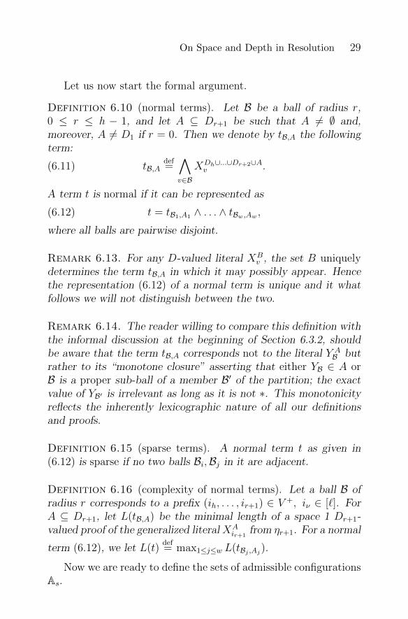
Definition 6.10 (normal terms). Let B be a ball of radius r,0 ≤ r ≤ h − 1, and let A ⊆ Dr+1 be such that A 6= ∅ and,moreover, A 6= D1 if r = 0. Then we denote by tB,A the followingterm:

(6.11) tB,Adef=∧v∈B

XDh∪...∪Dr+2∪Av .

A term t is normal if it can be represented as

(6.12) t = tB1,A1 ∧ . . . ∧ tBw,Aw ,where all balls are pairwise disjoint.

Remark 6.13. For any D-valued literal XBv , the set B uniquely

determines the term tB,A in which it may possibly appear. Hencethe representation (6.12) of a normal term is unique and it whatfollows we will not distinguish between the two.

Remark 6.14. The reader willing to compare this definition withthe informal discussion at the beginning of Section 6.3.2, shouldbe aware that the term tB,A corresponds not to the literal Y A

B butrather to its “monotone closure” asserting that either YB ∈ A orB is a proper sub-ball of a member B′ of the partition; the exactvalue of YB′ is irrelevant as long as it is not ∗. This monotonicityreflects the inherently lexicographic nature of all our definitionsand proofs.

Definition 6.15 (sparse terms). A normal term t as given in(6.12) is sparse if no two balls Bi,Bj in it are adjacent.

Definition 6.16 (complexity of normal terms). Let a ball B ofradius r corresponds to a prefix (ih, . . . , ir+1) ∈ V +, iν ∈ [`]. ForA ⊆ Dr+1, let L(tB,A) be the minimal length of a space 1 Dr+1-valued proof of the generalized literal XA

ir+1from ηr+1. For a normal

term (6.12), we let L(t)def= max1≤j≤w L(tBj ,Aj).

Now we are ready to define the sets of admissible configurationsAs.


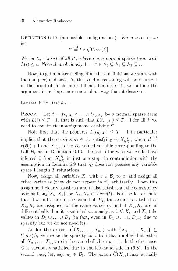
Definition 6.17 (admissible configurations). For a term t, welet

t∗def= t ∧ η[V ars(t)].

We let As consist of all t∗, where t is a normal sparse term withL(t) ≤ s. Note that obviously 1 = 1∗ ∈ A0 ⊆ A1 ⊆ A2 ⊆ . . ..

Now, to get a better feeling of all these definitions we start withthe (simpler) end task. As this kind of reasoning will be recurrentin the proof of much more difficult Lemma 6.19, we outline theargument in perhaps more meticulous way than it deserves.

Lemma 6.18. 0 6∈ AT−1.

Proof. Let t = tB1,A1 ∧ . . . ∧ tBw,Aw be a normal sparse termwith L(t) ≤ T − 1, that is such that L(tBj ,Aj) ≤ T − 1 for all j; weneed to construct an assignment satisfying t∗.

Note first that the property L(tBj ,Aj) ≤ T − 1 in particular

implies that there exists aj ∈ Aj satisfying ηd[XAji(j)], where d

def=

r(Bj) + 1 and Xi(j) is the Dd-valued variable corresponding to theball Bj as in Definition 6.16. Indeed, otherwise we could have

inferred 0 from XAji(j) in just one step, in contradiction with the

assumption in Lemma 6.9 that ηd does not possess any variablespace 1 length T refutations.

Now, assign all variables Xv with v ∈ Bj to aj and assign allother variables (they do not appear in t∗) arbitrarily. Then thisassignment clearly satisfies t and it also satisfies all the consistencyaxioms Cond(Xu, Xv) for Xu, Xv ∈ V ars(t). For the latter, notethat if u and v are in the same ball Bj, the axiom is satisfied asXu, Xv are assigned to the same value aj, and if Xu, Xv are indifferent balls then it is satisfied vacuously as both Xu and Xv takevalues in D1 ∪ . . . ∪ Dd (in fact, even in D1 ∪ . . . ∪ Dd−1 due tosparsity but we do not need it).

As for the axioms C(Xu1 , . . . , Xuw) with Xu1 , . . . , Xuw ⊆V ars(t), we invoke the sparsity condition that implies that eitherall Xu1 , . . . , Xuw are in the same ball Bj or w = 1. In the first case,

C is vacuously satisfied due to the left-hand side in (6.8). In the

second case, let, say, u1 ∈ B1. The axiom C(Xu1) may actually


come from an arbitrary level d, not necessarily the relevant oned = r(B1) + 1. But if d = r(B1) + 1, then C is an axiom of τd andhence is satisfied by a1 due to its choice. On the other hand, ifd 6= r(B1) + 1, then C(a1) = 1 simply because it becomes vacuousaccording to (6.8). Hence the assignment we have constructed sat-isfies η[V ars(t)] as well.

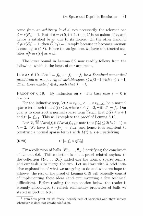
The lower bound in Lemma 6.9 now readily follows from thefollowing, which is the heart of our argument.

Lemma 6.19. Let 1 = f0, . . . , f1 . . . , fs be a D-valued semanticalproof from ηh·ηh−1·. . .·η1 of variable space≤ h/2−1 with s ≤ T−1.Then there exists f ∈ As such that f |= fs.

Proof of 6.19. By induction on s. The base case s = 0 isobvious.

For the inductive step, let t = tB1,A1 ∧ . . . ∧ tBw,Aw be a normalsparse term such that L(t) ≤ s, where s ≤ T−2, with t∗ |= fs. Ourgoal is to construct a normal sparse term t such that L(t) ≤ s+ 1and t∗ |= fs+1. This will complete the proof of Lemma 6.19.

Let7 V0def= V ars(fs)∪V ars(fs+1); note that |V0| ≤ 2(h/2−1) =

h − 2. We have fs ∧ η[V0] |= fs+1, and hence it is sufficient toconstruct a normal sparse term t with L(t) ≤ s+ 1 satisfying

(6.20) t∗ |= fs ∧ η[V0].

Fix a collection of balls B∗1, . . . ,B∗w∗ satisfying the conclusionof Lemma 6.6. This collection is not a priori related anyhow tothe collection B1, . . . ,Bw underlying the normal sparse term t,and our task is to merge the two. Let us start with a brief intu-itive explanation of what we are going to do and what we hope toachieve: the rest of the proof of Lemma 6.19 will basically consistof implementing these ideas (and circumventing a few technicaldifficulties). Before reading the explanation below, the reader isstrongly encouraged to refresh elementary properties of balls westated in Section 6.3.1.

7From this point on we freely identify sets of variables and their indiceswhenever it does not create confusion.


The terms tB1,A1 , . . . , tBw,Aw carry all the information our refuta-tion has been able to achieve so far and the balls B∗1, . . . ,B∗w∗ con-tain all variables that are kept in memory at the moment. UnlikeB1, . . . ,Bw, these latter balls are new-born and are not equippedwith any particular terms yet. Let us, however, postpone this issueand discuss geometry first.

Ideally, we would like to keep in the game all balls

(6.21) B1, . . . ,Bw,B∗1, . . . ,B∗w∗

but this is of course impossible because of potential conflicts be-tween them. These conflicts can be of one of the two types: con-tainment conflicts and adjacency conflicts.

Due to the fact that both collections of balls are individu-ally conflict-free (and B∗1, . . . ,B∗w∗ satisfies even a much strongerproperty), the picture is actually less chaotic than it may appearon the first glance. No ball in (6.21) may both contain anotherball and be (properly) contained in one. The adjacency relation,when restriced to (6.21), is a matching. Yet another importantobservation is that no ball in B1, . . . ,Bw may be involved in bothcontainment and adjacency conflicts. Indeed, if Bγ were in an adja-cency conflict with B∗µ and in a containment conflict with B∗µ′ then(B∗µ)+ ⊃ Bγ would have a non-empty intersection with B∗µ′ whichis impossible due to the way these balls were chosen (see the state-ment of Lemma 6.6). This may happen for a new ball B∗µ, though;this issue will be addressed when we will talk about designing setsA∗µ for those balls.

With these remarks in mind, we resolve all containment con-flicts in favor of the larger ball and remove the smaller. Adjacencyconflicts (Bγ,B∗µ) are always resolved in favor of B∗µ: Bγ gets re-

moved. This will define the geometry of the term t, it will benormal and sparse as we have resolved all conflicts, and it willcontain all variables in V0 due to the way we have resolved them.

It remains to explain how to transfer information from a termtBγ ,Aγ to the new generation of balls if Bγ was slated for extermina-tion, and we still have to define A∗µ for those new balls B∗µ. Thereare two reasons why Bγ can be removed: since Bγ ⊂ B∗µ for some µ(containment conflict) or because it is adjacent to some B∗µ. In the


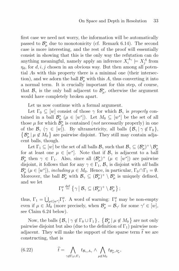
first case we need not worry, the information will be automaticallypassed to B∗µ due to monotonicity (cf. Remark 6.14). The secondcase is more interesting, and the rest of the proof will essentiallyconsist in showing that this is the only way the refutation can doanything meaningful, namely apply an inference X

Aγi |= XA

j fromηd, for d, i, j chosen in an obvious way. But then among all poten-tial As with this property there is a minimal one (their intersec-tion), and we adorn the ball B∗µ with this A, thus converting it intoa normal term. It is crucially important for this step, of course,that Bγ is the only ball adjacent to B∗µ, otherwise the argumentwould have completely broken apart.

Let us now continue with a formal argument.Let Γ0 ⊆ [w] consist of those γ for which Bγ is properly con-

tained in a ball B∗µ (µ ∈ [w∗]). Let M0 ⊆ [w∗] be the set of allthose µ for which B∗µ is contained (not necessarily properly) in oneof the Bγ (γ ∈ [w]). By ultrametricity, all balls Bγ | γ 6∈ Γ0,B∗µ | µ 6∈M0

are pairwise disjoint. They still may contain adja-

cent balls, though.Let Γ1 ⊆ [w] be the set of all balls Bγ such that Bγ ⊆ (B∗µ)+\B∗µ

for at least one µ ∈ [w∗]. Note that if Bγ is adjacent to a ballB∗µ then γ ∈ Γ1. Also, since all (B∗µ)+ (µ ∈ [w∗]) are pairwisedisjoint, it follows that for any γ ∈ Γ1, Bγ is disjoint with all ballsB∗µ (µ ∈ [w∗]), including µ ∈M0. Hence, in particular, Γ0∩Γ1 = ∅.Moreover, the ball B∗µ with Bγ ⊆ (B∗µ)+ \ B∗µ is uniquely defined,and we let

Γµ1def=γ∣∣ Bγ ⊆ (B∗µ)+ \ B∗µ

;

thus, Γ1 =.⋃µ∈[w∗]Γ

µ1 . A word of warning: Γµ1 may be non-empty

even if µ ∈ M0 (more precisely, when B∗µ = Bγ′ for some γ′ ∈ [w],see Claim 6.24 below).

Now, the balls Bγ | γ 6∈ Γ0 ∪ Γ1 ,B∗µ | µ 6∈M0

are not only

pairwise disjoint but also (due to the definition of Γ1) pairwise non-adjacent. They will make the support of the sparse term t we areconstructing, that is

(6.22) t =∧

γ 6∈Γ0∪Γ1

tBγ ,Aγ ∧∧µ6∈M0

tB∗µ,A∗µ ,


where for µ 6∈ M0 the sets A∗µ are defined as follows. Let µ 6∈ M0

and rdef= r(B∗µ).

Case 1. r(Bγ) < r for any γ ∈ Γµ1 (which in particularincludes the case Γµ1 = ∅).

We simply let A∗µdef= Dr+1 unless r = 0 in which case, due to

our convention, we simply remove tB∗µ,A∗µ from (6.22).

Case 2. There exists γ ∈ Γµ1 with r(Bγ) = r.First note that γ with this property is unique since t is sparse.

Bγ and B∗µ are defined by two prefixes of the form (ih, ih−1, . . . , ir+2, i)and (ih, ih−1, . . . , ir+2, j) with i 6= j. We let A∗µ be the minimal sub-set of Dr+1 for which

(6.23) XAγi ∧ η[Xi, Xj] |= X

A∗µj

in the Dr+1-valued logic. We note that L(tBµ,A∗µ) ≤ s+1 and hence(this is quite essential for the upcoming argument!) A∗µ 6= ∅ due tothe assumption s ≤ T − 2.

This completes the construction of the sparse term t, and allthat remains is to prove (6.20). Let us first state formally a fewobservations that we already made in our informal explanationabove.

Claim 6.24. If Γµ1 6= ∅ then t contains a sub-term of the formtB∗µ,A for some A.

Proof of 6.24. If µ 6∈ M0, this is obvious. If µ ∈ M0 thenB∗µ ⊆ Bγ for some γ and there is another γ′ with Bγ′ ⊆ (B∗µ)+ \ B∗µ.We necessarily must have B∗µ = Bγ (otherwise, Bγ′ ⊆ Bγ). Clearly,

γ 6∈ Γ0 ∪ Γ1 and hence tBγ ,Aγ = tB∗µ,Aγ appears in t.

Claim 6.25. V0 ⊆ V ars(t).

Proof of 6.25. Every v ∈ V0 is contained in one of the ballsB∗µ. If µ 6∈ M0, we are done, otherwise there exists γ ∈ [w] withB∗µ ⊆ Bγ. Like in the proof of Claim 6.24, γ 6∈ Γ0∪Γ1, hence tBγ ,Aγappears in t and thus v ∈ V ars(t).


As an immediate consequence, the second part of the implica-tion in (6.20) is automatic, and we only have to prove that t∗ |= fs.Again, let us begin with a simple observation.

Claim 6.26. Let α be an arbitrary assignment satisfying a termtB,A of the form (6.11). Then α satisfies all axioms Conρ(u,v)(xu, xv) (u, v ∈B) if and only if α is constant on B.

Proof of 6.26. By an easy inspection.

Our strategy for proving t∗ |= fs given that V ars(fs) ⊆ V ars(t)(by Claim 6.25) and t∗ |= fs is typical for this kind of argumentsin proof complexity. Namely, fix an assignment α ∈ V D satisfyingt∗. In order to prove that fs(α) = 1, we only have to show how tomodify α to another assignment β such that:

1. α and β agree on V0;

2. t∗(β) = 1.

This β will be obtained from α by the “reverse engineering”of the intuition for the construction of t we provided above. Theterms tBγ ,Aγ with γ ∈ Γ0 will be trivially satisfied by monotonicity,we need not worry about them. If γ ∈ Γ1, i.e. Bγ is removed infavor of an adjacent ball B∗µ, then, due to the minimality in (6.23),every assignment a ∈ A∗µ can be extended to an assignment b ∈ Aγsatisfying the left-hand side, and we use this b to re-assign variablesin the ball Bγ.

Formally, consider an individual Bγ, γ ∈ Γµ1 and let rdef= r(B∗µ).

By Claim 6.24, B∗µ ⊆ V ars(t), and then by Claim 6.26 (since αsatisfies η[B∗µ]), α|B∗µ is a constant a with a ∈ Dh ∪ . . .∪Dr+2 ∪A∗µ.

Case 1. a ∈ Dh ∪ . . . ∪Dr+2.We simply let β|Bγ ≡ a.

Case 2.1. a ∈ A∗µ and r(Bγ) = r, i.e., Bγ and B∗µ are adjacent.In the notation of (6.23), there exists b ∈ Aγ such that η[Xi, Xj](b, a) =

1; otherwise a could have been removed from A∗µ in violation ofthe minimality of (6.23). Pick arbitrarily any such b and defineβ|Bγ ≡ b.


Case 2.2. a ∈ A∗µ, r(Bγ) < r.We let β|Bγ ≡ b, where b ∈ Dr(Bγ)+1 is chosen in such a way

that η[Xi](b) = 1. Here, as before, i is the last entry in the prefixdescribing the ball Bγ.

The construction of β is complete.

Claim 6.27. α and β agree on all balls B∗µ and on all balls Bγ (γ 6∈Γ1).

Proof of 6.27. Follows from the above remarks that the ballsBγ (γ ∈ Γ1) are disjoint from anything else.

In particular, α and β agree on V0, and it remains to show thatt∗(β) = 1.

First we check that t(β) = 1, that is tBγ ,Aγ (β) = 1 for anyγ ∈ [w]; this part is relatively easy and was already sufficientlyexplained above. There are three possibilities.

Case 1. γ ∈ Γ0.We have Bγ ⊂ B∗µ for some µ 6∈ M0, and by Claim 6.27, α and

β coincide on B∗µ. Since r(Bγ) ≤ r(B∗µ)−1, we have tB∗µ,A∗µ |= tBγ ,Aγregardless of the particular value of A∗µ (over which we do not have

any control). But tB∗µ,A∗µ appears in t and hence tB∗µ,A∗µ(α) = 1.tBγ ,Aγ (β) = 1 follows.

Case 2. γ ∈ Γ1.In this case tBγ ,Aγ (β) = 1 directly follows from the way the

assignment β was constructed.

Case 3. γ 6∈ Γ0 ∪ Γ1.Once again, α and β coincide on Bγ, and tBγ ,Aγ also appears in

t. Hence tBγ ,Aγ (β) = 1.

So far we have proved t(β) = 1, and what still remains is toshow that η[V ars(t)](β) = 1, i.e., we should take care of the “en-vironment” of the term t. This part is technically unpleasant, wehave tried several natural possibilities (like modifying the predicate|= in the statement of Lemma 6.19 to pertain to legal assignmentsonly), and none of them has been fully satisfactory. Perhaps, thebest intuition towards the remaining part of the proof below is


that we have defined both the “forward” construction t =⇒ t andthe “reverse” one α =⇒ β as natural as possible so that the “sup-plementary” information contained in η[V ars(t)] “floats around”both ways. Let us at least briefly explain a (typical) example ofthe constraint Cond(Xu, Xv), where u ∈ Bγ, v ∈ Bγ′ and γ 6= γ′.A problem occurs when at least one of the balls Bγ,Bγ′ is removed,and, moreover, when it is removed due to an adjacency conflict(containment conflicts only increase V ars(t)). If, say, Bγ is re-moved in favor of an adjacent ball B∗µ 6⊇ Bγ′ , then we will still havethat ρ(B∗µ,Bγ′) = ρ(Bγ,Bγ′) = d and hence our constraint Condstill makes perfect sense (and the same content, too) between B∗µand Bγ′ . We replace Xu in it with Xu∗ , where u∗ ∈ B∗µ is arbitrary,and show that Cond(αu∗ , βv) = 1 implies Cond(βu∗ , βv) = 1. An-other kind of care should be given to constraints of width 1, forthe same reasons as in the proof of Lemma 6.18, but perhaps atthis point it will be simpler just to start the formal argument.

Let us fix C ∈ η with V ars(C) ⊆ V ars(t). We need to provethat

(6.28) C(β) = 1.

Case 1. V ars(C) ⊆ Bγ for some γ.

Let rdef= r(Bγ).

Case 1.1. C = C0(Xu, Xv) (u, v ∈ Bγ), where C0 ∈ ηd, ddef=

ρ(u, v).This case is immediate from the already established fact t(β) =

1 since it implies βu, βv ∈ Dh ∪ . . . ∪Dr+1, while d ≤ r.

Case 1.2. C = Conρ(u,v)(Xu, Xv).For every ball B occurring in the right-hand side of (6.22), α|B

is constant by Claim 6.26 since α satisfies all consistency axiomsConρ(u,v)(Xu, Xv) with u, v ∈ B ⊆ V ars(t). Following the samereasoning as in the proof of t(β) = 1 above, β|Bγ is also a constanthence C(β) = 1 by Claim 6.26.

So far we have treated axioms C of width 2 with V ars(C) ⊆ Bγ.We divide the analysis of the case when C is of width 1 into twosubcases, according to whether γ ∈ Γ1 or not.


Case 1.3. C = C0(Xu), where C0 ∈ ηd for some d and γ 6∈ Γ1.Since Xu ∈ V ars(t), C(αu) = 1, and since γ 6∈ Γ1, C(βu) =

C(αu). This gives (6.28).

Case 1.4. C = C0(Xu), where, as before, C0 ∈ ηd for some dbut γ ∈ Γ1.

Let γ ∈ Γµ1 and Rdef= r(B∗µ) ≥ r. From our construction,

either α|B∗µ ∈ Dh ∪ . . . ∪ DR+2 and β|Bγ ≡ α|B∗µ , or b ∈ Dr+1 andη[Xi](b) = 1, where i is again the last entry in the prefix describingBγ.

Case 1.4.1. β|Bγ ≡ α|B∗µ ∈ Dh ∪ . . . ∪DR+2 (= a).We may assume d ≥ R+2 as otherwise the statement is trivial.

Pick arbitrarily u∗ ∈ B∗µ, then ρ(u, u∗) = R + 1. Hence u and u∗

share the prefix of length h−d ≤ h−R−2, that is C0(Xu∗) is also

in η. Now C0(a) = 1 follows from Xu∗ ∈ V ars(t).

Case 1.4.2. b ∈ Dr+1 and η[i](b) = 1.Again, this is obvious if d 6= r+1 and follows from C0 ∈ ηd[i]

otherwise.

We have completed the analysis of the case V ars(C) ⊆ Bγ fora single ball Bγ. In particular, we can and will now assume thatthe width of the constraint C is exactly 2:

Case 2. V ars(C) = u, v, u ∈ Bγ and v ∈ Bγ′ with γ 6= γ′.

Let ddef= ρ(u, v), r

def= r(Bγ), r′

def= r(Bγ′), so that r, r′ ≤ d − 1

and, moreover, at least one of this inequalities is strict (since theballs Bγ, Bγ′ are non-adjacent).

Case 2.1. γ 6∈ Γ1 and γ′ 6∈ Γ1.This case is immediate: βu = αu, βv = αv and (6.28) simply

follows from the fact that α satisfies η[V ars(t)].

Case 2.2. γ ∈ Γ1.

Let γ ∈ Γµ1 and Rdef= r(B∗µ) so that R ≥ r. Let also a

def= α|B∗µ ;

a ∈ Dh ∪ . . . ∪DR+1.The rest of the analysis splits into two rather different cases

according to whether v ∈ (B∗µ)+ or not.

Case 2.2.1. v ∈ (B∗µ)+, that is d ≤ R + 1.


Case 2.2.1.1. a ∈ Dh ∪ . . . ∪DR+2.According to the construction, βu = βv = a. Cond(βu, βv) = 1

follows immediately, and for C0(βu, βv) (C0 ∈ τd) we only have toremark that a 6∈ Dd since d ≤ R + 1.

Case 2.2.1.2. a ∈ DR+1.

Case 2.2.1.2.1. v ∈ B∗µ.From our construction, d = R + 1, βv = a, and βu ∈ Dr+1.

Thus, βu, βv ∈ Dd ∪ . . . ∪D1, and this proves Cond(βu, βv) = 1, as

well as C0(βu, βv) = 1 unless r = R, that is the balls Bγ and B∗µare adjacent. In this latter case C0(βu, a) = 1 is guaranteed by ourchoice of βu.

Case 2.2.1.2.2. v ∈ (B∗µ)+ \ B∗µ. In this case γ′ ∈ Γµ1 as well,and, according to our construction, βu ∈ Dr+1 and βv ∈ Dr′+1.Recalling that r + 1, r′ + 1 ≤ d and, moreover, at least one of theinequalities here is strict, both Cond(βu, βv) and C0(βu, βv) (C0 ∈τd) are satisfied for trivial reasons.

At this moment, we are done with the case v ∈ (B∗µ)+.

Case 2.2.2. v 6∈ (B∗µ)+ or, in other words, d ≥ R + 2.Pick arbitrarily u∗ ∈ B∗µ. Since ρ(u, u∗) = R + 1, by the ul-

trametric triangle inequality we get ρ(u∗, v) = d. In particular,C(Xu∗ , Xv) is also an axiom of η.

Claim 6.29. C(βu, βv) = C(αu∗ , βv).

Proof of 6.29. Readily follows from the dichotomy βu = βu∗ =αu∗ or βu, αu∗ ∈ DR+1 ∪ . . . ∪D1 ⊆ Dd−1 ∪ . . . ∪D1.

Thus, if γ′ 6∈ Γ1 then u∗, v ⊆ V ars(t), βv = αv and we are done

since α satisfies t∗. On the other hand, if γ′ ∈ Γµ′

1 for some µ′ 6= µthen u∗ 6∈ (B∗µ′)+, and we simply apply Claim 6.29 once more, thistime with u = v, v = u∗, u∗ = v∗, where v∗ ∈ B∗µ′ .

This finally completes our case analysis. To re-cap the over-all argument, we have proved (6.28) for any axiom C ∈ η withV ars(C) ⊆ V ars(t). That is, for any assignment α ∈ DV witht∗(α) = 1 we were able to modify it to some β ∈ V D so that α andβ agree on V0 and t∗(β) = 1. This implies (6.20) and completesthe inductive step.


As we observed above, the lower bound in Lemma 6.9 follows im-mediately.

6.4. From multi-valued logic to the Boolean one. Finally,we need to transfer the tradeoff resulting from Lemmas 6.3, 6.9 tothe Boolean setting. This involves two different tasks: the con-version per se and a variable compression in the style of Razborov(2016) that is certainly needed here since the number of variablesin the lexicographic product is huge (exponential in h). We willcombine both tasks into a single statement, but first we need a fewdefinitions.

Definition 6.30 (Alekhnovich & Razborov 2008). A functiong : 0, 1s −→ D is r-surjective if for any restriction ρ assigning atmost r variables, the restricted function g|ρ is surjective.

Definition 6.31 (cf. Razborov 2016). Let A be an m × n 0-1matrix in which every row has precisely s ones and g : 0, 1s −→D be a function. Let g[A] : 0, 1n −→ Dm be naturally definedas

g[A](x1, . . . , xn)(i)def= g(xj1 , . . . , xjs),

where j1 < j2 < . . . < js is the enumeration of ones in the ithrow of A. For a D-valued Boolean function f : Dm −→ 0, 1,we let the Boolean function f [g, A] : 0, 1n −→ 0, 1 be thecomposition f g[A]. Finally, for a D-valued CSP η(Y1, . . . , Ym),

we let η[g, A]def= C[g, A] | C ∈ η.

Definition 6.32. Let A be a m× n 0-1 matrix. For i ∈ [m], let

Ji(A)def= j ∈ [n] | aij = 1

be the set of all ones in the ith row. For a set of rows I ⊆ [m], theboundary ∂A(I) of I is defined as

∂A(I)def= j ∈ [n] | | i ∈ I | j ∈ Ji(A) | = 1 ,

i.e., it is the set of columns that have precisely one 1 in theirintersections with I. A is an (r, c)-boundary expander if |∂A(I)| ≥c|I| for every set of rows I ⊆ [m] with |I| ≤ r.


Lemma 6.33. Let A be an m× n(2h, 3

4s)-boundary expander in

which every row has precisely s elements. Let D be a finite domain,η(Y1, . . . , Ym) be a D-valued h-CSP and g : 0, 1s −→ D be an(3s/4)-surjective function. Assume that there exists a semantic(Boolean) refutation π from η[g, A] with VSpace(π) ≤ (hs)/16.Then there exists a D-valued refutation π of η with VSpace(π) ≤ hand |π| = |π|.

Proof. In the notation of this lemma, fix a semantical (Boolean)refutation π = (f0, . . . , fT ) from η[g, A] with VSpace(π) ≤ (hs)/16.In order to convert π to a D-valued refutation, we need to recall afew rudimentary facts about expanders.

Definition 6.34. For a set of columns J ⊆ [n], let

Ker(J)def= i ∈ [m] | Ji(A) ⊆ J

be the set of rows completely contained in J . Let A \ J be thesub-matrix of A obtained by removing all columns in J and allrows in Ker(J).

The following is a part of (Razborov 2016, Lemma 4.4).

Proposition 6.35. Let A be an (m×n) (r, c)-boundary expanderin which every row has at most s ones, let c′ < c, and let J ⊆ [n]

satisfy |J | ≤ r2(c− c′). Then there exists J ⊇ J such that A \ J is

an (r/2, c′)-boundary expander and |J | ≤ |J |(1 + s

c−c′).

We now return to the proof of Lemma 6.33. Let8 Jtdef= V ars(ft);

|Jt| ≤ (hs)/16. Apply to this set Proposition 6.35 with r = 2h, c =

3s/4 and c′ = 5s/8. We will get Jt ⊇ Jt such that A \ Jt is an

(h, 5s/8)-boundary expander and |Jt| ≤ 9|Jt| ≤ 9hs/16. Let Itdef=

Ker(Jt); we claim that |It| ≤ h. Indeed, assuming the contrary,

pick a set I ′t ⊆ It with |I ′t| = h. Then |∂A(I ′t)| ≤ |Jt| ≤ 9hs/16,contrary to the fact that A is an (h, 3s/4)-boundary expander.

8Recall that we often identify sets of variables with sets of their indices.


We now let ft be the minimal D-valued function in the variablesyi | i ∈ It such that

(6.36) ft |= ft[g, A]

in the Boolean logic. Then∣∣∣V ars(ft)∣∣∣ ≤ h and all that remains to

show is that (f0, f1, . . . , fT ) is indeed a D-valued semantic refuta-tion, that is

(6.37) ft ∧ η[It ∪ It+1] |= ft+1,

for all t.

Let α ∈ Dm be any assignment satisfying the left-hand side in(6.37). Due to the minimality of ft, if we re-define it to 0 on theinput α|It , this will violate (6.36). In other words, there exists aBoolean assignment a ∈ 0, 1n such that ft(a) = 1 and

(6.38) g(a|Ji(A)

)= αi,

for any i ∈ It. We note that these two properties of a depend onlyon those values aj for which j ∈ Jt; thus, we can view a as an

assignment in 0, 1Jt , discarding all other values. Our goal is to

extend a to an assignment in 0, 1Jt∪Jt+1 in such a way that (6.38)will be satisfied for all i ∈ It+1 as well.

This is done by a fairly standard argument. Let Idef= It+1 \ It.

Since A\Jt is an (h, 5s/8)-boundary expander and |I| ≤ |It+1| ≤ h,

we have∣∣∣∂A(I) \ Jt

∣∣∣ ≥ 5s8|I|. Hence for at least one i ∈ I,∣∣∣∣∣∣Ji(A) \

Jt ∪ ⋃i′∈I\i

Ji′(A)

∣∣∣∣∣∣ ≥ 5s

8≥ s

4.

Removing this i from I and arguing by reverse induction, we canorder all rows in I in such a way I = i1, i2 . . . , ir that

(6.39)∣∣∣Jiν (A) \

(Jt ∪ Ji1(A) ∪ . . . ∪ Jiν−1(A)

)∣∣∣ ≥ s

4


for all ν = 1..r. Using now (3s/4)-surjectivity of g, we consecu-

tively extend a to Jt∪Ji1(A)∪ . . .∪Jiν (A) enforcing all conditions(6.38).

The partial assignment a ∈ 0, 1Jt∪Jt+1 we have constructed

still satisfies ft; we claim that it also satisfies η[g, A][Jt ∪ Jt+1

]⊇

η[g, A][Jt ∪ Jt+1].Indeed, for any C ∈ η[It∪It+1] this simply follows from the fact

that C(α) = 1 and the consistency conditions (6.38). One thing we

still have to make sure is that η[g, A][Jt ∪ Jt+1

]does not contain

any other, “accidental” constraints.

Claim 6.40. If C is any constraint of width≤ h and V ars(C[g, A]) ⊆Jt ∪ Jt+1 then V ars(C) ⊆ It ∪ It+1.

Proof of 6.40. By a relatively simple modification of the ar-

gument above. Let Idef= V ars(C); |I| ≤ h, and assume the con-

trary, that is that there exists i ∈ I \ (It ∪ It+1). Fix two assign-ments α, β ∈ DI differing only in the ith coordinate but such thatC(α) 6= C(β). We claim that there exist a, b ∈ 0, 1n such that(cf. (6.38))

(6.41) g(a|Ji(A)

)= αi, g

(b|Ji(A)

)= βi,

for all i ∈ I while a|Jt∪Jt+1= b|Jt∪Jt+1

: the first property will imply

C[g, A](a) 6= C[g, A](b), and that will contradict V ars(C[g, A]) ⊆Jt ∪ Jt+1 by the second property.

We construct the promised a, b in two stages. Let I ′def= I∩ (It∪

It+1); thus, α and β agree on I ′. As before, order the rows in I ′ insuch a way I ′ = I1, . . . , Ir that∣∣Jiν (A) \ (Ji1(A) ∪ . . . ∪ Jiν−1(A))

∣∣ ≥ s/4

holds for all ν (cf. (6.39)), and then satisfy (6.41) with the same

assignment to Ji1(A)∪. . .∪Jir(A). Extend it to Jt∪Jt+1 arbitrarily;

let c ∈ 0, 1Jt∪Jt+1 be the resulting assignment.

Now, let I ′′def= I \ (It∪ It+1), and let A∗ be the matrix obtained

from A by removing all columns Jt, Jt+1 and all rows It, It+1. Since


both A\Jt and A\Jt+1 are (h/2, 5s/8)-expanders, clearly A∗ is stillan (h, s/4)-expander ( s

4= 2 ·

(58s)− s). This expansion property

allows us to extend c, by the same argument as above, to a, b ∈0, 1n that will satisfy (6.41) for i ∈ I ′′ as well. But, as weremarked above, (6.41) is in contradiction with V ars(C[g, A]) ⊆Jt ∪ Jt+1.

Since η is an h-CSP by the assumption of Lemma 6.33, we canapply Claim 6.40 to any C ∈ η. This gives us that all constraints

in η[g, A][Jt ∪ Jt+1

]are indeed coming from η[It ∪ It+1]. As we

already remarked above, this implies that all of them are satis-fied by the assignment a, and since (f0, f1, . . . , fT ) is a semanticalrefutation from τ [g, A], we conclude that ft+1(a) = 1. By (6.36),

ft+1[g, A] = 1, and since a satisfies (6.38) for all i ∈ It+1, this

means ft+1(α) = 1.

We have established (6.37) by showing that any D-valued as-signment α satisfying its left-hand side also satisfies the right-handside. Thus, (f0, f1, . . . , fT ) is indeed a semantical refutation. Thiscompletes the proof of Lemma 6.33.

6.5. Putting it all together.

Proof of 3.3. We are given a function s = s(n) ≤ n1/2. We

let hdef= bεsc ≤ εn/s, where ε is a sufficiently small constant. We

now need the following standard fact:

Proposition 6.42 (Razborov 2016, Lemma 2.2). Let n → ∞and m, s, c be arbitrary integer parameters possibly depending onn such that c ≤ 3

4s and

(6.43) r ≤ o(n/s) ·m−2s−c .

Then for sufficiently large n there exist m× n (r, c)-boundary ex-panders in which every row has ≤ s ones.

Note that (6.43) is satisfied with m := 4h, c := 34s and r := 2h (the

term m−2s−c becomes Ω(1)). This gives us an (2h, 3

4s)-boundary

expander with m = 4h rows in which every row has ≤ s ones. By


adding ≤ s extra columns if necessary, we can assume w.l.o.g. thatevery row has exactly s ones.

Next, we claim that if s is sufficiently large (that we can clearlyassume w.l.o.g.) a random function g : 0, 1s −→ D is (3s/4)surjective for |D| = 2s/8, with probability 1−o(1). This is straight-forward:

P[g is not (3s/4)− surjective]

≤ 23s/4

(s

3s/4

)P[g|ρ is not surjective]

≤ exp(O(s)) · (1− |D|−1)2s/4 ≤ o(1),

where ρ is a fixed restriction assigning (3s/4) variables. Pickany such g arbitrarily, and split D into h nearly equal parts,D = D1

.∪ . . .

.∪ Dh. Let ηd be the Dd-valued 2-CSP in four vari-

ables given by Lemma 6.3, that is such that VSpace(ηd ` 0) = 1but any its refutation π with VSpace(π) = 1 must have length

≥ exp(|Dd|Ω(1)

)≥ exp(exp(Ω(s))). Let η

def= ηh · . . . · η1. The

D-valued 2-CSP η has m = 4h variables, say, Y1, . . . , Ym and stillsatisfies VSpace(η ` 0) = 1 but now any its refutation π withVSpace(π) ≤ h/2− 1 has length exp(exp(Ω(s))). The desired con-tradiction τn will be η[g, A].

First of all, τn has a semantical refutation with variable space≤ s. It is obtained simply by taking a D-valued refutation of ηwith variable space 1 (that is, consisting of generalized literals) andapplying the operator Y P

i 7→ Y Pi [g, A] to its configurations. On the

other hand, applying Lemma 6.33 in the contrapositive form, everyBoolean refutation π from ηg[A] with VSpace(π) ≤ (h/2 − 1)s/16must have length ≥ exp(exp(Ω(s)))/ exp(O(h)). As h = Θ(s), thisis exp(exp(Ω(s))).

7. Conclusion

In this paper we have studied two complexity measures of propo-sitional proofs, variables space and depth, that in our view havebeen somewhat neglected in the past. We hope that perhaps thenature of the results proved in this paper would help them to find


the place in the overall hierarchy that, in our opinion, they fullydeserve by the token of being very clean, robust and natural.

That said, the most interesting question about them remainsopen: whether variable space and depth are polynomially relatedor, equivalently, whether there exists a supercritical tradeoff be-tween them. In a slightly less precise form this was asked in(Urquhart 2011, Problem 7.2); we have proved a quadratic gap,but the general problem looks quite challenging.

A positive answer to this question would immediately implythat clause space is polynomially bounded by variable space. Evenif these two problems seem to be extremely tightly related, we stillwould like to ask this separately: is it correct that

CSpace(τn ` 0) ≤ (VSpace(τn ` 0) log n)O(1)?

In the opposite range, of (barely) constant variable space, allrefutations a priori have small length, and we have shown that thedepth can be reduced to, say, n while keeping the variable spaceconstant and length polynomial. We would like to take this oppor-tunity and re-iterate an interesting question of (somewhat) similarflavor asked in (Nordstrom 2013, Open Problem 16). Assume thatwe have a configurational refutation of constant clause space. Is italways possible to reduce length to polynomial while keeping theclause space constant? As with our first question, this one alsolooks quite challenging.

Finally, there still remains a considerable amount of work to bedone on refining simulations in Theorem 3.1. For example, let ustake a closer look at (1.6). By Bonacina’s result (1.5), every O(1)-CNF τn with w(τn ` 0) = Θ(n) automatically provides an examplewith TSpace(τn ` 0) = Θ(D2) (= Θ(n2)). But what about thelower bound in (1.6)? Can, say, TSpace be sub-linear in depth or

the bound can be improved to Ω(D)? This does not seem to easilyfollow from any known results.

Acknowledgements

This work was supported by the Russian Science Foundation, grant# 14-50-00005.


The author is deeply indebted to anonymous referees of thispaper for constructive criticism and a great deal of very usefulremarks.

References

M. Alekhnovich, E. Ben-Sasson, A. Razborov & A. Wigderson(2002). Space complexity in propositional calculus. SIAM Journal onComputing 31(4), 1184–1211.

M. Alekhnovich & A. Razborov (2008). Resolution is not autom-atizable unless W [P ] is tractable. SIAM Journal on Computing 38(4),1347–1363.

A. Atserias & V. Dalmau (2008). A combinatorial characterizationof resolution width. Journal of Computer and System Sciences 74(3),323–334.

L. Babai & A. Seress (1992). On the Diameter of PermutationGroups. European Journal of Combinatorics 13, 231–243.

B. Barak & D. Steurer (2014). Sum-of-squares proofs and the questtoward optimal algorithms. In Proceedings of International Congress ofMathematicians (ICM), volume IV, 509–533.

C. Beck, J. Nordstrom & B. Tang (2013). Some trade-off resultsfor polynomial calculus: extended abstract. In Proceedings of the 45thACM Symposium on the Theory of Computing, 813–822.

E. Ben-Sasson (2009). Size-space tradeoffs for resolution. SIAM Jour-nal on Computing 38(6), 2511–2525.

E. Ben-Sasson & A. Wigderson (2001). Short Proofs are Narrow -Resolution made Simple. Journal of the ACM 48(2), 149–169.

C. Berkholz & J. Nordstrom (2016a). Near-Optimal Lower Boundson Quantifier Depth and Weisfeiler-Leman Refinement Steps. In Pro-ceedings of the 31st Annual ACM/IEEE Symposium on Logic in Com-puter Science, 267–276.

C. Berkholz & J. Nordstrom (2016b). Supercritical Space-WidthTrade-offs for Resolution. In Proceedings of the 43rd International Col-loquium on Automata, Languages and Programming, 57:1–57:14.


A. Blake (1937). Canonical expressions in Boolean algebra. Ph.D.thesis, University of Chicago.

I. Bonacina (2016). Total space in Resolution is at least width squared.In Proceedings of the 43rd International Colloquium on Automata, Lan-guages and Programming, 56:1–56:13.

S. A. Cook & A. R. Reckhow (1979). The relative efficiency ofpropositional proof systems. Journal of Symbolic Logic 44(1), 36–50.

J. L. Esteban & J. Toran (2001). Space bounds for resolution.Information and Computation 171(1), 84–97.

Y. Filmus, M. Lauria, M. Miksa, J. Nordstrom & M. Vinyals(2015). From Small Space to Small Width in Resolution. ACM Trans-actions on Computational Logic 16(4), article 28.

D. Grigoriev (2001). Linear lower bounds on degrees of Postivestel-lensatz calculus proofs for the parity. Theoretical Computer Science259, 613–622.

J. Nordstrom (2013). Pebble Games, Proof Complexity and Time-Space Trade-Offs. Logical Methods in Computer Science 9, 1–63.

A. Razborov (2016). A New Kind of Tradeoffs in Propositional ProofComplexity. Journal of the ACM 62(3), article 16.

A. Razborov (2017). On the Width of Semi-AlgebraicProofs and Algorithms. Mathematics of Operation ResearchHttp://pubsonline.informs.org/doi/abs/10.1287/moor.2016.0840.

J. A. Robinson (1965). A machine-oriented logic based on the resolu-tion principle. Journal of the ACM 12(1), 23–41.

A. Urquhart (2011). The Depth of Resolution Proofs. Studia Logica99, 349–364.

Manuscript received 7 December 2016

Alexander RazborovUniversity of ChicagoChicago IL 60637, [email protected]

Steklov Mathematical InstituteMoscow 117418 [email protected].

on space and depth in resolution -...

Documents