on the combination of graph data for assessing thin- le
TRANSCRIPT

On the combination of graph data for assessing thin-fileborrowers’ creditworthiness
Ricardo Munoz-Cancino1, Cristian Bravo2, Sebastian A. Rıos3, and Manuel Grana4
1,3Business Intelligence Research Center (CEINE), Industrial Engineering Department, University ofChile, Beauchef 851, Santiago 8370456, Chile
2Department of Statistical and Actuarial Sciences, The University of Western Ontario,1151 RichmondStreet, London, Ontario, N6A 3K7, Canada.
4Computational Intelligence Group, University of Basque Country, 20018 San Sebastian, Spain.
Abstract
The thin-file borrowers are customers for whom a creditworthiness assessment is uncertaindue to their lack of credit history; many researchers have used borrowers’ relationships andinteractions networks in the form of graphs as an alternative data source to address this.Incorporating network data is traditionally made by hand-crafted feature engineering, andlately, the graph neural network has emerged as an alternative, but it still does not improveover the traditional method’s performance. Here we introduce a framework to improve creditscoring models by blending several Graph Representation Learning methods: feature engi-neering, graph embeddings, and graph neural networks. In this approach, we stacked theiroutputs and trained a gradient boosting classifier to produce a single score. We validated thisframework using a unique multi-source dataset that characterizes the relationships, interac-tions, and credit history for the entire population of a Latin American country, applying it tocredit risk models, application and behaviour, targeting both individuals and companies. Ourresults show that the graph representation learning methods should be used as complements,and these should not be seen as self-sufficient methods as is currently done. In terms of AUCand KS, we enhance the creditworthiness assessment statistical performance, outperformingtraditional methods to incorporate graph data. In Corporate lending, where the gain is muchhigher, it confirms that evaluating an unbanked company cannot solely consider its character-istics. The business ecosystem where these companies interact with their owners, suppliers,customers, and other companies provides novel knowledge that enables financial institutionsto enhance their creditworthiness assessment. Our results let us know when and on whichpopulation to use graph data and what effects on performance to expect. They also show theenormous value of graph data on the unbanked credit scoring problem, principally to helpcompanies’ banking.
Keywords: Credit Scoring; Machine Learning; Social Network Analysis; Network Data;Graph Neural Networks
∗NOTICE: Changes resulting from the publishing process, such as peer review, editing, corrections, structural formatting, andother quality control mechanisms may not be reflected in this version of the document. This work is made available under a CreativeCommons BY-NC-ND license. cbnd
1
arX
iv:2
111.
1366
6v1
[cs
.SI]
26
Nov
202
1

1 Introduction
A large part of the population requires access to credit to achieve their life goals: social mobility,obtaining their own home, and the desired financial success. Moreover, access to financial servicesand a proper credit evaluation can facilitate and often be necessary to obtain a job, rent a home,buy a car, start a new business, and pursue a college education (Aziz and Dowling, 2019; Hurleyand Adebayo, 2017). At the macroeconomic level, access to credit is an indispensable driver forlocal economic growth, especially in developing economies (Diallo and Al-Titi, 2017). Financialinstitutions play a significant role by being the ones who facilitate access to credit, assuming therisk that this entails. To manage this credit risk, financial institutions have applied credit scoringfor decades to assess the creditworthiness of their borrowers; this to distinguish between goodand bad payers and, in this way, deliver loans to those most likely to repay. To build a creditscoring model, financial institutions use personal information, banking data, and payment historyto estimate creditworthiness and avoid granting credit to people with a high probability of default.Despite being the standard mechanism in the industry, not only for credit-granting decisions butalso for managing the loan life-cycle (Thomas et al., 2017), this ubiquitous tool still does not assureadequate access to credit and the financial system.
The world bank calculates that more than 1.7 billion remain unbanked, adults without accessto the financial system (The Global Financial Index, 2017). This number only considers those whodo not have a bank account either through a financial institution or mobile banking. If we includedthe underbanked, those who have an account but cannot apply for a loan, this number would bemuch higher. Being unbanked or underbanked presents the lack of credit history, also known asthin-file borrowers, meaning that people cannot obtain a load for being bad payers but rather lackthe attributes to be evaluated by traditional credit scoring models (Baidoo, 2020; Cusmano, 2018;Djeundje et al., 2021; Hurley and Adebayo, 2017).
Under this scenario, lenders have tried different ways of reaching this population; we mainlyhighlight two business models. The traditional business model, where the higher risk assumed dueto the lack of information, is compensated by applying higher interest rates. Alternatively, reachingthis population by granting microcredits has been used as a strategy to know the client’s paymentbehavior under limited exposure. However, neither of these solutions has proven to be cost-efficientto address this population (Baidoo, 2020; Hurley and Adebayo, 2017). For this reason, in recentyears, financial institutions, fintech, and researchers have innovated in their business models andin making better decisions with the available information; therefore, they have developed betteralgorithms and incorporated alternative data sources to improve credit scoring models. Multiplelines of research have been established; some of them attempt to understand the characteristics ofdefaulters (Bravo et al., 2015) or the feature selection process (Maldonado et al., 2017; Verbrakenet al., 2014). However, the most significant improvements have been obtained in the inclusionof alternative data sources such as telephone call data (Oskarsdottir et al., 2018a; Oskarsdottiret al., 2019,1), written risk assessments (Stevenson et al., 2021), data generated by an app-basedmarketplace (Roa et al., 2021a,2), social media data (Cnudde et al., 2019; Masyutin, 2015; Putraet al., 2020), network information (Ruiz et al., 2017), the role of the family (Okten and Osili,2004), social surveys (Silver, 2001), fund transfers dataset (Shumovskaia et al., 2020; Sukharevet al., 2020) or psychometric data (Rabecca et al., 2018; Shoham, 2004). One of the main aspectsof the studies presented above is the use network data, the graph formed of the interactions amongindividuals recorded in alternative data sources. Based on our research, we have mainly identifiedtwo gaps that we will address in this work. The first gap is the data sources employed. Most ofthe studies are carried out with partial networks that fail to capture all of the interactions. These
2

networks are limited by the data provider. Our study will use the network data information tocharacterize the interactions of the country’s entire population, having a complete vision of thefinancial system. On the other hand, the network’s knowledge extraction is mainly done throughhand-made feature engineering (Freedman and Jin, 2017; Lin et al., 2013; Oskarsdottir et al., 2019;Ruiz et al., 2017; Wei et al., 2016), and in recent years through graph neural networks (Roa et al.,2021b) but without better results than the traditional feature engineering approach.
Our work will study the combination of different representation learning techniques over com-plex graph structures in a complementary approach rather than understanding the different tech-niques as substitutes. Hence, our investigation will seek answers to the following questions:
1. When combining different Graph Representation Learning techniques over complex graphsstructures, Is there a performance improvement compared to merely applying hand-craftedfeature engineering or graph neural networks?
2. What insights are obtained of the combined network features, and what value do they addto credit risk assessment?
3. Where does graph information help the most? Is the most significant performance enhance-ment obtained in which problem, personal credit scoring or business credit scoring? Whatcan we gather from this? Does it influence which network and which features are the mostrelevant?
This study challenges the traditional hand-crafted feature engineering and the novel graph neu-ral network approach by combining multiple graph representation learning methods. In particular,our work contributes to the following aspects.
• We introduce a framework to combine traditional hand-engineered features with Graph Em-beddings and Graph Neural Networks features. This framework produces a single score,facilitating its users to decide to approve or reject a credit.
• Our results are the first to validate and test graph data over both corporate and consumerlending, showing that the information from graphs has a different effect depending on theborrower analyzed, people, or companies; these effects are reflected in the predictive powerenhancement and in which features are relevant in each problem. Knowing this is importantsince it lets us know when and on which population to use graph data and what effects onperformance to expect.
• To the best of our knowledge, this is the first study that incorporates the credit behavior ofan entire country, together with networks that allow characterizing its entire population andconsolidate multiple types of social and economic relationships: parental, marital, businessownership, employment, and transactional services.
• This paper also contributes to growing literature in credit scoring and network data, propos-ing a mechanism to achieve better results than the popular hand-crafted feature engineeringand the novel graph neural network approach.
This study is structured as follows. Section 2 presents a review of credit risk management,credit scoring and social networks, and graph representation learning methods. Section 4 showsthe description of the data sources and features. Section 5 shows the proposed methodology, andthe experimental design adopted. Section 6 presents the results obtained. The conclusions andfuture work that originated from this research are presented in Section 7.
3

2 Literature review
2.1 Credit Risk Management
Banks core business is granting loans to individuals and companies. Granting a loan is an actionthat is not risk-free; in fact, Banks are heavily exposed to credit risk (Apostolik et al., 2009),originated from the potential loss due to the default of their debtors or their inability to complywith the agreed conditions (The Basel Committee on Banking Supervision, 2000). Banking riskmanagement focuses on detecting, measuring, reporting, and managing all sources of risk. Banksdefine strategies, policies, and procedures to keep the risk they assume limited to achieve this goal.These strategies encourage and integrate the use of mathematical models for the early detectionof potential risks. Credit Scoring is the widely used tool for managing credit risk, allows tohandle large volumes of data and captures patterns that are complex to express as business rules.This instrument became popular and ubiquitous in the 80s mainly due to advances in computingpower and the growth of financial markets, making it almost impossible to manage large creditportfolios without this kind of tools; since then, credit scoring models have been used by mostfinancial institutions to manage credit risk (Thomas et al., 2017). The regulatory framework alsoendorses the use of credit scoring models; in fact, the Basel Accords allow banks to manage creditrisk with internal ratings; specifically, banks develop internal models for assessing the expectedloss. The expected loss assessment can be decomposed into three components: the probabilityof default (PD), the loss given default (LGD), and the exposure at default (EAD), being theprobability of default a key component, due is used to define the granting credit policies and forportfolio management. The general approach to estimating the PD and assessing the borrower’screditworthiness is through classification techniques using demographics features and the paymenthistory as explanatory variables. Over the years, lenders have explored multiple ways to improvecreditworthiness assessment, novel machine learning techniques (Lessmann et al., 2015), and non-traditional data sources (Aziz and Dowling, 2019).
There are multiple forms to classify credit scoring problems. A classification adopted foracademics and practitioners is to distinguish between application scoring and behavior scoring.First, the application scoring corresponds to a credit scoring system for new customers, where theinformation available is often scarce and limited. Behavioral scoring is also a credit scoring systemfor borrowers with available credit and repayment history. In this work, both credit scoring typesand their differences between people and businesses will be studied.
2.2 Credit Risk and Social Networks
The inclusion of alternative data in the credit scoring problem has gained relevance in recentyears. We define graph data as that information that records the relationships or interactionsamong entities. In this way, a network corresponds to a group of nodes in which edges connectpairs of nodes. In this study, the nodes represent people or companies, and the edges representthe multiple kinds of interaction between them. We will refer to a network as a Social Networkwhen nodes are people or companies, and edges denote any social interaction like friendship,acquaintances, neighbors, colleagues, or affiliation to the same group (Easley and Kleinberg, 2010).Mathematically, we describe a network by a graph G(V,E,A), V is the set of nodes and E is the setof edges. Let V = {v1, . . . , vN} where |V | = N is the number of nodes, and the adjacency matrixA ∈ R|V |×|V | with Aij = 1 if there is an edge eij from vi to vj, Aij = 0 otherwise. Additionally,graph can be associated with a node attributes matrix X ∈ RN×F , where Xi ∈ RF represents the
4

feature vector of node vi.The emerging credit scoring and network data literature have focused on incorporating hand-
crafted features into a traditional credit scoring problem. In this line of research, we highlight thework developed by Oskarsdottir et al. (2016) and Oskarsdottir et al. (2018,1). The authors incor-porate network information into the customer churn problem, using eight telco datasets originatingfrom around the world. This series of studies outlined the foundations for the incorporation ofnetwork data in credit scoring. The application in credit scoring of this framework is carried out inOskarsdottir et al. (2018a,1); Oskarsdottir et al. (2019), where the authors introduce a methodologyto enhance smartphone-based credit scoring models’ predictive power through feature engineeringfrom a pseudo-social network, combining social network analysis and representation learning. Dueto that, it is feasible to increase the performance of micro-lending smartphone applications gener-ating a high helping potential for financial inclusion. An extension of this work is to measure creditrisk’s temporal and topological dynamics, i.e., how it evolves and spreads in the graph. For this,Bravo and Oskarsdottir (2020) implemented modifications to the PageRank algorithm to quantifythis phenomenon. This methodology allows them to quantify the risk of the different entities in amultilayer network. Their results show how the risk of default spreads and evolves over a networkof agricultural loans. Then, Oskarsdottir and Bravo (2021) analyzed how to build the multilayernetwork, interpret the variables derived from it, and incorporate this knowledge in credit risk man-agement. Their results reveal that the default risk increases as a debtor presents links with manydefaulters; however, this effect is mitigated by the size of each individual’s neighborhood. Theseresults are significant as they indicate that default and financial stability risk spread through thenetwork.
Other works have used a graph convolutional network-based approach for this purpose. Shu-movskaia et al. (2020) present one of the first empirical works with massive graphs created fromtransactions between clients of a large Russian bank. They propose a framework to estimate linksusing SEAL (Zhang and Chen, 2018) and Recurrent Neural Networks, the SEAL-RNN framework.One of the advantages of using SEAL is that it focuses only on the link’s neighborhood to bepredicted, and it does not use the entire graph as in Graph Convolutional Networks. This allowsscaling the analysis to massive graphs, 86 million nodes, and 4 billion edges. Despite not beinga methodology for default prediction, the authors extend their research and apply it to a creditscoring problem. Sukharev et al. (2020) propose a method to predict the default from a moneytransfer network and the historical information of transactions. To work with both datasets, theypropose a methodology based on Graph Convolutional Networks and Recurrent Neural Networks tohandle network data and transactional data, respectively. As baseline models, they train a modelwith 7000 features; however, they achieved an increase of 0.4% AUC when compared the proposedmodel with the best baseline model. Finally, Roa et al. (2021a) present a methodology for us-ing alternative information in a credit scoring model. Models are estimated using data generatedby an app-based marketplace; this information is precious for low-income segments and youngindividuals, who are often not well assessed by traditional credit scoring models. The authorscompare a model with hand-crafted features versus models from graph convolutional networks.However, the approach with graph convolutional networks does not achieve better results thanusing hand-crafted features in terms of predictive power.
5

3 Representation Learning on Networks
The machine learning subfield that attempts to apply techniques to graph-structured data is knownas Graph Representation Learning (Hamilton et al., 2017). Unlike the traditional tabular data,the complexity of network data imposes a challenge to conventional machine learning algorithms;therefore, it is not possible to use it directly, generating changes either in the algorithms or inthe data representation. These challenges are mainly since the network information is, in essence,unstructured. In fact, operations easy to calculate on other data types, such as convolutions onimages, cannot be applied directly to graphs due each node has a variable number of neighbors.Researchers have proposed many methodologies to extract knowledge for networks; here, we presenta nomenclature and the characteristics for the primary methods.
3.1 Feature Engineering
Data preparation is one of the most critical steps in any analytical project before training anymachine learning model. Formulating accurate and relevant features is critical to improving modelperformance (Nargesian et al., 2017). Regarding the use of graph data, the traditional featureengineering approach consists of characterizing each node either based on the aggregation of itsneighborhood’s features or the node’s statistics within the network.
3.2 Network Embeddings
Network embedding methods are unsupervised learning techniques aiming to learn a Euclideanrepresentation of networks in a much lower dimension. Mapping each node into a Euclidean spaceis done through the optimization of similarity functions. The distance between network nodes inthe new space is a surrogate for the node’s closeness within the network structure. Among theadvantages of node embedding techniques is that they replace feature engineering processes.
Formally, a network is represented by a graph G(V,E,A) which is defined by a set of nodesV , a set of edges E and an adjacency matrix A ∈ R|V |×|V |. A node embedding is a functionf : G(V,E,A) → Rd that maps each node v ∈ V to an embedding vector {Zv}v∈V ∈ Rd (Arsovand Mirceva, 2019) preserving the adjacency in the graph, i.e. the feature vectors of pairs ofnodes that are connected by an edge are more similar than those that are disconnected. LetZ ∈ R|V |×d denote the node embedding matrix where d � |V | for scalability purposes. Themost popular Network Embedding method is Node2vec (Grover and Leskovec, 2016), which is analgorithmic framework to learn low-dimensional network representation. This algorithm maximizesthe probability of preserving the neighborhood of the nodes in the embedding subspace. Theyoptimize, using stochastic gradient descent, a network-based objective function, and producedsamples for neighborhoods of nodes through second-order random walks. The key feature ofNode2vec is the use of biased-random walks, providing a trade-off among two network searchmethods: breadth-first search (BFS) and depth-first search (DFS); this trade-off creates moreinformative network embeddings than other competing methods.
3.3 Graph neural networks (GNN)
Graph-structured data have arbitrary structures that can can vary significantly between networksor within different nodes of the same network. Their support domain is not a uniformly discretizedEuclidean space. For this reason, the convolution operator often used for signal processing cannot
6

be directly applied to graph-structured data. Geometric Deep Learning (GDL) and Graph NeuralNetworks (GNN) aim to modify, adapt and create deep learning techniques for non-Euclidean data.The proposed GDL computational schemes are an adaptation of deep autoencoders, convolutionalnetworks, and recurrent networks to this particular data domain. In this study we will be applyingGraph Convolutional Networks (GCN) and Graph Autoencoders (GAE).
3.3.1 Graph Convolutional Networks
The graph convolutional neural networks (GCNs) generalize the convolution operation to networksformalized as graphs. GCNs aims to produce a node’s representation Zv by adding its attributesor feature vector Xv and neighbors {Xu}u∈N(v), where N(v) is the ego network of node n, i.e., thesubgraph composed of the nodes to whom node n is connected. This study will use the spectral-based GCN, aka Chebyshev Spectral convolutional neural network, proposed by Defferrard et al.(2016), which defines the graph convolution operator as a filter from graph signal processing. Inparticular, we will use the specific GCN proposed by (Kipf and Welling, 2016a) which uses as afilter a first-order approximation of the Chebyshev polynomial of the eigenvalues’ diagonal matrix.This GCN operation follows the expression:
Xi ∗ gθ = θ0Xi − θ1D− 1
2AD−12Xi, (1)
where Xi is the feature vector, gθ is a function of the eigenvalues of the normalized graph Laplacianmatrix L = In − D−
12AD−
12 , A is the adjacency matrix, Dij =
∑j Ai,j, ∀i, j ∈ V : i = j, and
θ is the vector of Chebyshev coefficients. In the following we summarize the derivation of thisfirst-order approximation Kipf and Welling (2016a).
3.3.2 Derivation of GCN from spectral methods
Spectral methods are founded on a solid theoretical basis defined for graph signal processing meth-ods developed essentially from the Laplacian matrix properties. To build up the graph convolutionoperator, we start from the normalized graph Laplacian matrix defined as follows:
L = In −D−12AD−
12 , (2)
where A is the adjacency matrix, and Dij =∑
j Ai,j, ∀i, j ∈ V : i = j. Because L is a real,symmetric, and positive semi-defined matrix, we can rewrite L as a function of its eigenvectormatrix U and its eigenvalues λi, i.e. L = UΛUT , where U ∈ RN×N , and Λij = λi, ∀i, j ∈ V : i = j.
The next step is to define the graph Fourier transform and its inverse. The graph Fouriertransform F of the feature vector Xi ∈ X is defined as follows:
F(Xi) = UTXi, (3)
where X is the matrix of node attributes, and the inverse Fourier transform of a graph is definedas follows:
F−1(Xi) = UXi, (4)
where Xi are the coordinates of the nodes in the new space; therefore the feature vector can bewritten as Xi =
∑jinV Xiuj. Finally, the graph convolution of feature vector Xi with filter g ∈ RN ,
using the element-wise product �, is defined as follows:
Xi ∗ g = F−1(F(Xi)�F(g)) (5)
7

One of the most popular filters is the Chebyshev polynomial of the eigenvalues’ diagonal matrix,i.e. gθ = diag(UTg) =
∑K θkTk(Λ), where Λ = 2λ/λmax − I and the polynomials Tk are defined
as Tk(x) = 2xTk−1 − Tk−2(x), with T0(x) = 1 and T1(x) = x. Therefore, the graph convolutionalnetwork, the Chebyshev Spectral CNN (Defferrard et al., 2016), takes the form:
Xi ∗ gθ =∑K
θkTk(L)Xi, (6)
where L = 2L/λmax − I. Despite being a graph convolution simplification, this convolution iscomputationally expensive for large graphs. To solve this, Kipf and Welling (2016a) present afirst-order approximation of the Chebyshev Spectral CNN (GNC). Assuming K = 1 and λmax = 2, the equation 5 takes the form:
Xi ∗ gθ = θ0Xi − θ1D− 1
2AD−12Xi (7)
3.3.3 Graph autoencoders (GAEs)
Graphs autoencoders (GAE) are an unsupervised method that allows obtaining a low-dimensionalrepresentation of the network. The objective of the GAE is to reconstruct the original network usingthe same network for this task, which is encoded, reducing its dimensionality, and then decoded toreconstruct the network. The encoded representation is used as the network embedding. Wu et al.(2020) distinguish two main uses of Graph Autoencoders, namely Graph Generation and NetworkEmbedding. This research will use GAEs in order to obtain a lower-dimensional vector preservingthe network topology (Network Embedding).
The already defined GCN is the building block of the GAE architecture, which allows tosimultaneously encode the network topology and the attributes of the nodes. GAE (Kipf andWelling, 2016b) calculates the network embedding matrix Z and the reconstruction of the originalnetwork adyacency matrix A as follows:
A = σ(ZZT ), with Z = GCN(X,A), (8)
where X is the matrix of node attributes, and A is the network’s adjacency matrix.
4 Data Description
The data used in this paper encompases several datasets provided by a large Latin American bank;some datasets contain information from their customers, while others concern the entire populationof the country.
4.1 Ethical and privacy protection Considerations
The datasets contain anonymized information and do not compromise the identity of any customeror its personal information in any way. The datasets share an anonymized customer’s id allowingus to merge multiple sources. Regarding the value, importance, and sensitivity of the data, we haveapplied multiple actions to ensure their security, integrity, and confidentiality. Customer identifiersand any personal data were removed before starting the analysis, and there is no possibility thatthis investigation can leak any personal private information. Also, any final data produced as aresult of this research do not compromise customers’ privacy.
8

4.2 Social Interaction Data
The information collected by the financial institution in order to build up the social network back-ground information of the thin file borrower originates from varied sources and can be catalogedas follows:
• [WeddNet] Network of marriages: This network is built from the information of mar-riages recorded by the bureau of vital statistics from 1938 to December 2015. It includes theanonymized identifier of the husband and the wife and the date of the wedding.
• [TrxSNet] Transactional services Network: The primary source of this network comesfrom transactional services data, primarily transfers of funds between two entities and payrollservices. We have access to monthly data from January 2017 to December 2019.
• [EnOwNet] Enterprise’s ownership Network: This network is built from the informa-tion on the ownership structure of companies. For each firm, we have information concerningtheir owners, whether they are individuals or other firms. We have quarterly informationfrom January 2017 to November 2019.
• [PChNet] Parents & Children Network: This network corresponds to parental rela-tionships, where for every person born between January 1930 and June 2018, we have theanonymized identifiers of their parents.
• [EmpNet] Employment Network: This network is built from multiple sources and con-nects people with their employers. We have monthly data from January 2017 to December2019.
4.3 Financial Data
The node dataset contains information on the consolidated indebtedness of each of the debtors inthe Financial System from January 2018 until March 2020, and it monthly reports debt decom-position from 7.65 million people and 245,000 firms. We will refer to the features extracted fromthis dataset as Node features. Additionally, for every person and firm in the previous dataset, wehave access to the BenchScore, which corresponds to the probability of default for the coming12 months. This probability was assessed and provided by the financial institution, and it will beour benchmark to contrast the performance of our models.
4.4 Network Construction
It is possible to build a network from each of the data sources indicated in Section 4.2. However,not all of these networks are full fledged social networks. To manage this, we combine theminto two primary data sources. From them, we construct networks that characterize people andbusinesses.
[FamilyNet] Family Network: This network is formed of the combination of the Network ofMarriages (WeddNet) and the Parent & Children Network (PChNet). For the construction of thisnetwork, we use all the historical information available until the beginning of the analysis period,and no further information is included. In this way, the network remains unvarying throughoutthe study. We will call this type of network a static network.
9

[EOWNet] Enterprise’s ownership Network and Workers: This network is composedof the fusion of the Transactional services Network (TrxSNet), the Enterprise’s ownership Network(EnOwNet), and the Employment Network (EmpNet). This network attempts to represent thebusiness ecosystem where companies, business owners, and employees interact. Based on thesedata sources, a series of networks are generated, each network for each one of the 24 months forwhich we have information available, including the information collected up to the last day of thecorresponding month. We call this type of network a temporal network, because nodes and edgeschange over time.
5 Experimental Design and Methodology
5.1 Datasets
The credit scoring models are built with information about the financial system for 24 months.However, the models are trained over 23 months since the first month is held out for the featureextraction process (presented below in Section 5.3) in order to avoid target leakage (Kaufman et al.,2012). For the unbanked application scoring model, individuals and companies are considered onlyin the month that they enter the financial system. In contrast, for the behavioral scoring modelindividuals and companies are considered six or more months after entering the financial system.Table 1 summarizes the scoring application, the model trained and the size of the dataset used.
Table 1: Description of datasetScoring application Model Observations # Features
Unbanked ApplicationScoring
Business Credit Score 29,044 687Personal Credit Score 192,942 1,283
Behavioral ScoringBusiness Credit Score 931,910 687Personal Credit Score 1,978,664 1,283
5.2 Target
The target event is ”becoming a defaulter” during the period of observation. Therefore, we onlytake into account individuals or businesses that are non-defaulters at the start of the period ofobservation. We dismiss entities that are defaulters at the very beginning of the observation. Aperson or company is considered a defaulter when they have payments past due date for 90 or moredays within twelve months starting from the observation point. Otherwise, they are considerednon-defaulters. The target vector, denoted by ydef , contains the actual information about thetarget event.
5.3 Traditional and Graph Representation Learning Features
Combining the node information from Section 4.3 and the network data from Section 4.2 make itpossible to generate a set of new characteristics through a feature extraction process. The sets ofcharacteristics generated are detailed below:
• [NodeStats] Node Statistics: collects node centrality statistics, namely, its Degree, De-gree Centrality, number of Triads, PageRank Score, Authority and Hub score given by theHits Algorithm (Kleinberg, 1999), and an indicator of whether the node is an articulationpoint.
10

• [EgoNet] EgoNetwork Agreggation: In this dataset, each node is characterized by theinformation of other nodes connected to it (Ego network). We refer the dataset as EgoNetAggregation Features when we apply some aggregation function to the characteristics ofthe nodes included in the Ego Network. Specifically, we apply the mean and SD in thisstudy as in Nargesian et al. (2017); Roa et al. (2021a) for each attribute in the NodeStatsdataset. Figure 1 shows how this process would be within the network; the colored blacknode corresponds to the target node, and the colored gray nodes belong to its Ego Network.Computing the EgoNet Aggregation Features assume that each connection in the EgoNethas the same importance. However, connections in Ego networks can be weighted. For thisreason, we compute the EgoNet Weighted Aggregation Features where the featuresof the neighboring nodes are weighted according to a measure of the relationship intensitymeasured by weighted average and SD of the NodeStats attributes. .
Figure 1: Network Features Example
• [N2V] Node2Vec Features: Node2Vec is an unsupervised method that only uses thenetwork structure to generate the graph embedding. For the static network FamilyNetNode2Vec is applied only once. A node is characterized by this embedding regardless of themoment it was sampled in the dataset. For temporal networks (EOWNet), Node2Vec has tobe recomputed every period because of the network changes. Each node is characterized withthe embedding corresponding to the month in which it was sampled in the dataset. Figure2 shows the process to obtain the embedding features applying Node2Vec. Each period, a
timet0 tn
train
f1(G1)
{Zv}v ∈ V1
train
f2(G2)
{Zv}v ∈ V2
train
fn(Gn)
{Zv}v ∈ Vn
... ...
sample sample sample sample
dataset
Figure 2: Node2Vec to Features
11
timet0 tn
train model apply
f(Go) f(G1)
{Zv}v ∈ V1
apply
f(G2)
{Zv}v ∈ V2
apply
f(Gn)
{Zv}v ∈ Vn
... ...
sample sample sample sample
dataset
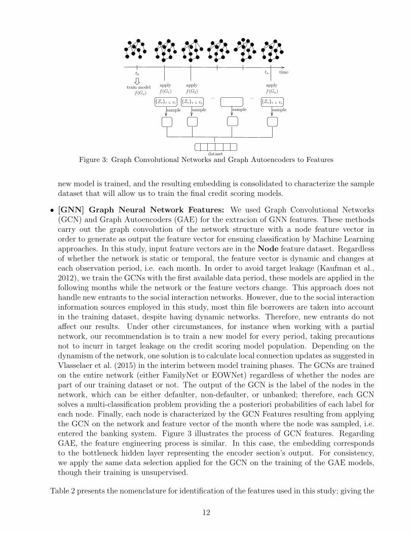
Figure 3: Graph Convolutional Networks and Graph Autoencoders to Features
new model is trained, and the resulting embedding is consolidated to characterize the sampledataset that will allow us to train the final credit scoring models.
• [GNN] Graph Neural Network Features: We used Graph Convolutional Networks(GCN) and Graph Autoencoders (GAE) for the extracion of GNN features. These methodscarry out the graph convolution of the network structure with a node feature vector inorder to generate as output the feature vector for ensuing classification by Machine Learningapproaches. In this study, input feature vectors are in the Node feature dataset. Regardlessof whether the network is static or temporal, the feature vector is dynamic and changes ateach observation period, i.e. each month. In order to avoid target leakage (Kaufman et al.,2012), we train the GCNs with the first available data period, these models are applied in thefollowing months while the network or the feature vectors change. This approach does nothandle new entrants to the social interaction networks. However, due to the social interactioninformation sources employed in this study, most thin file borrowers are taken into accountin the training dataset, despite having dynamic networks. Therefore, new entrants do notaffect our results. Under other circumstances, for instance when working with a partialnetwork, our recommendation is to train a new model for every period, taking precautionsnot to incurr in target leakage on the credit scoring model population. Depending on thedynamism of the network, one solution is to calculate local connection updates as suggested inVlasselaer et al. (2015) in the interim between model training phases. The GCNs are trainedon the entire network (either FamilyNet or EOWNet) regardless of whether the nodes arepart of our training dataset or not. The output of the GCN is the label of the nodes in thenetwork, which can be either defaulter, non-defaulter, or unbanked; therefore, each GCNsolves a multi-classification problem providing the a posteriori probabilities of each label foreach node. Finally, each node is characterized by the GCN Features resulting from applyingthe GCN on the network and feature vector of the month where the node was sampled, i.e.entered the banking system. Figure 3 illustrates the process of GCN features. RegardingGAE, the feature engineering process is similar. In this case, the embedding correspondsto the bottleneck hidden layer representing the encoder section’s output. For consistency,we apply the same data selection applied for the GCN on the training of the GAE models,though their training is unsupervised.
Table 2 presents the nomenclature for identification of the features used in this study; giving the
12

Table 2: Feature description and nomenclature. Due to the large number of generated features, wedescribe the nomenclature used for its name’s construction.
Feature Set Nomenclature Prefix/suffix Description
NodeFeatures(XNode)
Identifier NODEATT Feature subset identifier
Borrower featureidentifier
ATT01, · · · , ATT04 The debt situation characterized by thedelinquency level
ATT05, · · · , ATT08 The debt type: revolving, consumer,commercial, or mortgage
ATT09, · · · , ATT13Other aspects of the customer’s debt,payments in arrears, and the time inthe financial system
Bench Score The benchmark score
NodeStatistics
(XNodeStats)
Identifier NodeStats Feature subset identifier
Statistic identifier
DegreeCentr Degree centralityTriads Number of triads
PageRank PageRank AlgorithmArtPoint Articulation pointHits Auth Hits algorithm Authority scoreHits Hub Hits algorithm Hub score
Network identifierEOWNET EOWNet NetworkFamilyNet Family Network
EgoNetworkAgreggationFeatures(XEgoNet)
Borrower featureidentifier
ATT01, · · · , ATT13 Borrower Feature
Network identifierEOWNET EOWNet NetworkFamilyNet Family Network
AggregationFunction
MEAN MeanSTD Standard Deviation
EdgesFull All edges
NotBridge Edges that are not bridgesIsBridge Edges that are bridges
WeightedAggregations
Wby + Feature Suffix for weighted aggregations
Node2VecFeatures(XEgoNet)
Identifier N2V Feature subset identifierEmbeddingIdentifier
EMB 01, · · · , EMB 08 The embedding number
Network identifierEOWNET EOWNet NetworkFamilyNet Family Network
Graph NeuralNetworkFeatures(XGNN )
GNN IdentifierCHEB Graph Convolutional Network (GCN)GAE Graph Autoencoder
Borrower featureidentifier
01, · · · , 13 Borrower Feature
EmbeddingIdentifier
EMB 01, · · · , EMB nThe embedding number, where n = 3for CHEB and n = 8 for GAE
Network identifierEOWNET EOWNet NetworkFAMNET Family Network
necessary specifications for the correct interpretation of the attributes. For instance, the featuresthat will be the focus of later analysis are described below. New feature ids for the study variablesappear within brackets.
• [Egonet F01] EOWNetEgoNotBridge NET MEAN ATT13, calculated as the average Bench-mark Score of the company ego network, including only the non-bridge edges from theEOWNET Network.
• [Egonet F02] EOWNetEgoFull NET ATT07 Wby PageRank corresponds to the consumerdebt weighted by the PageRank of the node’s neighborhood in the EOWNET Network.
• [Egonet F03] FamilyNetEgoFull NET MEAN ATT 05, the unused revolving credit amountof the network, as the average neighborhood’s amount in the FamilyNet Network.
• [N2V F01] EOWNETGAE04 EMB 05 is a feature generated from a Graph Autoencodertrained with the consumer debt of the EOWNET Network
13

5.4 Features Subsets
The dataset is generated using the attributes defined in section 5.3, the subset A : XNode denotesthe dataset of characteristics of the node. B : XBenchScore is the Benchmark score; this attribute willalso be used as a benchmark to quantify our methodology’s contribution. The statistics obtainedfrom the position of the node within the network are denoted as C : XNodeStats. The feature setD : XEgoNet are the EgoNet Aggregation, and EgoNet Weighted Aggregation Features that arecalculated in three scenarios, considering the entire network, considering only those edges that arebridges, and finally considering those edges that are not bridges. An edge connecting the nodesu and v is called a bridge; if removing this edge, there is no longer a path connecting u andv. E : XGNN,N2V corresponds to the features created by applying Graph Neural Networks andNode2Vec. People are characterized with features from both networks, EOWNet and FamilyNet,while EOWNet only characterizes companies.
For this study, we grouped these features into eight incremental sets of information. The detailof these is presented below in Table 3.
Table 3: Experiments Setup
Experiment Id Feature Group
A X = {XNode}A+B X = {XNode + XBenchScore}A+B+C X = {XNode + XBenchScore + XNodeStats}A+B+D X = {XNode + XBenchScore + XEgoNet}A+B+E X = {XNode + XBenchScore + XGNN,N2V }A+B+C+D X = {XNode + XBenchScore + XNodeStats + XEgoNet}A+B+C+E X = {XNode + XBenchScore + XNodeStats + XGNN,N2V }A+B+C+D+E X = {XNode + XBenchScore + XNodeStats + XEgoNet + XGNN,N2V }
5.5 Methodology
The objective is to compare the predictive power of the features obtained through graph represen-tation learning techniques and to know the added value of each of them. For this, we propose thefollowing methodology.
First, a feature engineering process that seeks to create attributes to characterize the nodesfrom network data is carried out. Then, in the train-test split step, the available dataset is divided,a hyper-parameter training dataset (30% samples) to estimate the model’s hyper-parameters, andthe remaining samples (70% samples) are used to train and validate models with an N-Fold Cross-Validation scheme.
Before estimating the best hyper-parameters with the training set, we apply a feature selectionprocess. In this step, the intention is to choose a low-correlated subset of features with highpredictive power.
For this, three selection levels are formulated; the first is a bivariate selection that only considersa feature and the target and applies a threshold to this feature’s predictive power. In this firststep in the process, the variable is selected, only those variables such that KS > KSmin andAUC > AUCmin, where KSmin and AUCmin are parameters.
A multivariate selection is then applied; we developed a simple but effective method to dropcorrelated variables. This algorithm starts with an empty list S. We iterate over a set of featuresP in decreasing order of predictive power and append to S those features whose absolute value
14

of the correlation with all the features in S is less than a threshold ρ, this parameter is set toavoid high correlated features (Akoglu, 2018). The algorithm stops when all the features havebeen visited. The first feature in P is added to S without correlation comparison.
For this study, the multivariate selection process is applied twice; the first select low-correlatedfeatures for each group of attributes P ∈ {XNode ∪ XBenchScore, XNodeStats, XEgoNet, XGNN,N2V }.Then it is applied globally, considering all the remaining features P = {XNode ∪ XBenchScore ∪XNodeStats ∪ XEgoNet ∪ XGNN,N2V }. In both cases, a threshold ρ is used, and the features areordered by AUC, from higher to lower.
Finally, the N-Fold Cross-Validation stage, where the dataset is partitioned into N subset ofequal size. An iterative process over the N subsets begins, where the selected set is used as a testset, and a model is trained with the remaining N-1 subsets. The hyper-parameters used in eachiteration are the same and correspond to those estimated in the previous stage. Additionally, ineach of these iterations, multiple models are trained with different feature sets, which are storedand used later to compare the models.
5.6 Evaluation Metrics
The area under the receiver operating characteristic curve (AUC) is a popularly metric used toevaluate the model performance in classification problems (Bradley, 1997). It ranges between 0.5and 1; values closer to 1 indicate a better discriminatory capacity, while a value of 0.5 indicates adecision made by chance. In the context of credit scoring, the AUC can be easily interpreted asfollows: a defaulter and a non-defaulter are randomly selected, the AUC is the probability thatthe model assigns a higher score to the defaulter.
Another extensively utilized performance measure is the Kolmogorov-Smirnov (KS) statistic,which measures the distance separating the cumulative distributions of defaulters (PD(t)) andnon-defaulters (PND(t)) (Hodges, 1958). The KS statistic is defined as:
KS = maxt|PD(t)− PND(t)| (9)
KS ranges between 0 and 1, and similar to AUC a higher KS indicates a higher discriminatorycapacity.
5.7 Experimental setup
In this study, the methodology proposed in section 5 is used. The parameters of the univariateselection are set at KSmin = 0.01 and AUCmin = 0.53; for the multivariate selection process,ρ = 0.7 in both processes to avoid high correlated features (Akoglu, 2018). The N-Fold Cross-Validation stage is carried out considering N = 10, and in each iteration, the results of GradientBoosting (Friedman, 2001) models are displayed. Other classification models such as regularizedlogistic regression and Random Forest (Breiman, 2001) were trained. However, gradient boostingconsistently delivered better results.
6 Results and Discussion
In this section, we present the results obtained. We begin with the technical implementationdetails; then, we analyze the execution times. Subsequently, we display the model’s performancein three scenarios: the impact on performance using traditional features, the impact on performance
15

using the different graph representation methods, and the advantages of combining these methods.Finally, an analysis of the main features, traditional and network-based, for the creditworthinessassessment is presented.
6.1 Implementation Details
In this work we used Networkx v2.6.3 (Hagberg et al., 2008) and Snap-stanford v5.0.0 (Leskovec andSosic, 2016) Python implementations in the hand-crafted feature engineering process (XNodeStats,XEgoNet), and for Node2Vec, GCN and GAE (XGNN,N2V ) we used PyTorch v1.6.0 (Paszke et al.,2019) and PyTorch Geometric v2.0.1 (Fey and Lenssen, 2019).
To conduct the experiments, we used a laptop with 8 CPU cores Intel i7 and 32 GB of RAMfor network construction and hand-crafted feature engineering. We used a server with a drivernode with 140 GB of RAM and 20 CPU cores and between 2 and 8 auto-scaling worker nodes with112Gb of RAM and 16 CPU cores for the Node2Vec, GCN, GAE, and model training phase.
6.2 Execution Time
Below we detail the execution time of the most critical stages of our work, the implementation ofthe graph representation learning methods, and the models’ training.
• [NodeStats] Node Statistics: It corresponds to the computation of the metrics definedin section 5.3. This process is carried out only once for the static network FAMNET, and itis calculated for all the available periods (24) of the EOWNET. The computation of all themetrics for a network takes, on average, 25 minutes. The total execution time of this stepwas 625 minutes.
• [EgoNet] EgoNetwork Agreggation: It is calculated once per network type, FAMNETand EOWNET. The total execution time of this step was 300 minutes.
• [N2V] Node2Vec Features: This process is carried out only once for the static networkFAMNET, and it is calculated for all the available periods (24) of the EOWNET. TheNode2Vec training for a network takes, on average, 300 minutes. The total execution timeof this step was 7,500 minutes.
• [GNN] Graph Neural Network Features: In this process, eight models are trained usingeach network and eight different feature vectors. Each model training is carried out with thefirst available period data; then, it is applied to the remaining periods. Table 4 shows theexecution time by GNN type and by network type. The total execution time of this step was6,920 minutes.
• Gradient Boosting Training: Four models were trained using the methodology describedin section 5.5 for the scenarios defined in section 4, Application, and Behavioral Scoring forindividuals and companies. The complete training for each scenario takes, on average, 40minutes. The total execution time of this step was 160 minutes.
The total execution time of our methodology is 15,500 minutes. Although a large part of theseexecutions was parallelized using the server described in section 6.1, the high computational cost ismainly due to two factors, the volume of data and the complexity of the algorithms. Regarding thelarge volume of data, the FAMNET has 20 million nodes and 30 million edges, and the EOWNET
16
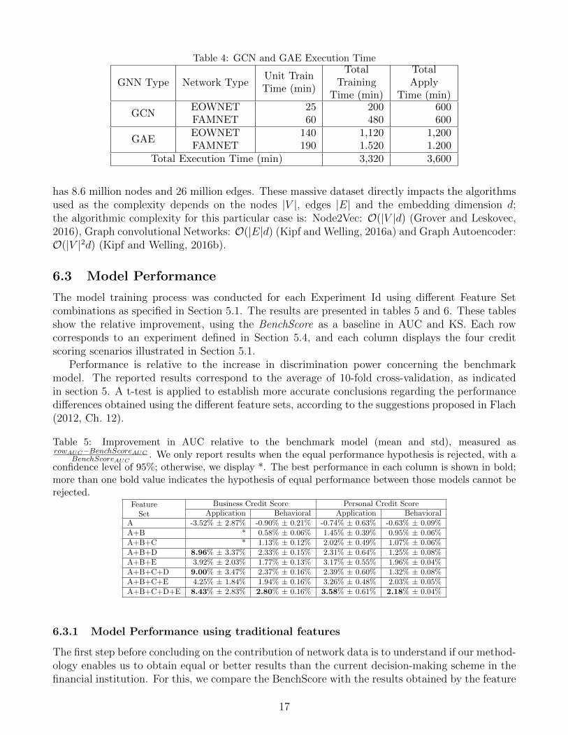
Table 4: GCN and GAE Execution Time
GNN Type Network TypeUnit TrainTime (min)
TotalTraining
Time (min)
TotalApply
Time (min)
GCNEOWNET 25 200 600FAMNET 60 480 600
GAEEOWNET 140 1,120 1,200FAMNET 190 1.520 1.200
Total Execution Time (min) 3,320 3,600
has 8.6 million nodes and 26 million edges. These massive dataset directly impacts the algorithmsused as the complexity depends on the nodes |V |, edges |E| and the embedding dimension d;the algorithmic complexity for this particular case is: Node2Vec: O(|V |d) (Grover and Leskovec,2016), Graph convolutional Networks: O(|E|d) (Kipf and Welling, 2016a) and Graph Autoencoder:O(|V |2d) (Kipf and Welling, 2016b).
6.3 Model Performance
The model training process was conducted for each Experiment Id using different Feature Setcombinations as specified in Section 5.1. The results are presented in tables 5 and 6. These tablesshow the relative improvement, using the BenchScore as a baseline in AUC and KS. Each rowcorresponds to an experiment defined in Section 5.4, and each column displays the four creditscoring scenarios illustrated in Section 5.1.
Performance is relative to the increase in discrimination power concerning the benchmarkmodel. The reported results correspond to the average of 10-fold cross-validation, as indicatedin section 5. A t-test is applied to establish more accurate conclusions regarding the performancedifferences obtained using the different feature sets, according to the suggestions proposed in Flach(2012, Ch. 12).
Table 5: Improvement in AUC relative to the benchmark model (mean and std), measured asrowAUC−BenchScoreAUC
BenchScoreAUC. We only report results when the equal performance hypothesis is rejected, with a
confidence level of 95%; otherwise, we display *. The best performance in each column is shown in bold;more than one bold value indicates the hypothesis of equal performance between those models cannot berejected.
FeatureSet
Business Credit Score Personal Credit ScoreApplication Behavioral Application Behavioral
A -3.52% ± 2.87% -0.90% ± 0.21% -0.74% ± 0.63% -0.63% ± 0.09%A+B * 0.58% ± 0.06% 1.45% ± 0.39% 0.95% ± 0.06%A+B+C * 1.13% ± 0.12% 2.02% ± 0.49% 1.07% ± 0.06%A+B+D 8.96% ± 3.37% 2.33% ± 0.15% 2.31% ± 0.64% 1.25% ± 0.08%A+B+E 3.92% ± 2.03% 1.77% ± 0.13% 3.17% ± 0.55% 1.96% ± 0.04%A+B+C+D 9.00% ± 3.47% 2.37% ± 0.16% 2.39% ± 0.60% 1.32% ± 0.08%A+B+C+E 4.25% ± 1.84% 1.94% ± 0.16% 3.26% ± 0.48% 2.03% ± 0.05%A+B+C+D+E 8.43% ± 2.83% 2.80% ± 0.16% 3.58% ± 0.61% 2.18% ± 0.04%
6.3.1 Model Performance using traditional features
The first step before concluding on the contribution of network data is to understand if our method-ology enables us to obtain equal or better results than the current decision-making scheme in thefinancial institution. For this, we compare the BenchScore with the results obtained by the feature
17

Table 6: Improvement in KS relative to the benchmark model (mean and std), measured asrowKS−BenchScoreKS
BenchScoreKS. We only report results when the equal performance hypothesis is rejected, with
a confidence level of 95%; otherwise, we display *. The best performance in each column is shown in bold;more than one bold value indicates the hypothesis of equal performance between those models cannot berejected.
FeatureSet
Business Credit Score Personal Credit ScoreApplication Behavioral Application Behavioral
A * -4.15% ± 0.94% -5.25% ± 2.40% -2.39% ± 0.46%A+B * 1.56% ± 0.40% 4.38% ± 1.19% 1.95% ± 0.35%A+B+C * 3.21% ± 0.71% 6.27% ± 1.02% 2.23% ± 0.39%A+B+D 20.69% ± 16.73% 7.69% ± 0.92% 6.79% ± 1.36% 2.69% ± 0.47%A+B+E 12.22% ± 10.89% 5.83% ± 0.74% 8.64% ± 2.13% 4.68% ± 0.28%A+B+C+D 21.28% ± 17.10% 8.09% ± 0.95% 7.12% ± 1.52% 2.83% ± 0.52%A+B+C+E 12.88% ± 10.11% 6.33% ± 0.70% 8.93% ± 1.98% 4.93% ± 0.26%A+B+C+D+E 19.32% ± 14.77% 9.45% ± 0.85% 10.83% ± 1.98% 5.15% ± 0.42%
set A+B. A comparison only with the feature set A is not entirely accurate, considering we donot have access to all the features used in the BenchScore training.
The results show that our methodology obtains equal or greater performance, measured interms of AUC and KS statistics, in all four scenarios; three of them are greater, with statisticallysignificant differences.
These performance enhancements in the Behavioral Business Credit Scoring problem are 0.58%and 1.56% for AUC and KS, respectively. For Personal Credit Scoring, the performance enhance-ments are AUC: 1.45%, KS: 4.38% for Application Scoring and AUC: 0.95%, and KS: 1.95% forBehavioral Scoring. These results indicate that using our methodology and training a model withsimilar features to the benchmark model can obtain better results than the current decision schemeutilized by the financial institution.
6.3.2 Model Performance using Graph Representation Learning features
In Application Business Credit Scoring, nearly a 9% AUC increase over the BenchScore is achieved.These results are obtained by a model that incorporates three feature sets: A+B+D, A+B+C+D,and A+B+C+D+E. Note that in these three sets, the common attributes correspond to thetraditional features A+B : XNode ∪ XBenchScore and EgoNet Aggregation Features D : XEgoNet.The performance comparison between all feature sets is shown in Table 7; we marked as * thosecomparisons with no statistically significant differences.
Table 7: Business Application Scoring performance comparison. Performance is measured by the relativeincrease in AUC ( rowAUC−columnAUC
columnAUC).
BENCH A A+B A+B+C A+B+D A+B+E A+B+C+D A+B+C+E A+B+C+D+E
BENCH * 3.65% * * -8.23% -3.77% -8.26% -4.08% -7.77%A -3.52% * -2.92% -4.55% -11.45% -7.16% -11.49% -7.45% -11.01%A+B * 3.01% * -1.68% -8.79% -4.37% -8.83% -4.67% -8.34%A+B+C * 4.77% 1.71% * -7.23% -2.73% -7.26% -3.04% -6.77%A+B+D 8.96% 12.94% 9.64% 7.79% * 4.85% * 4.52% *A+B+E 3.92% 7.71% 4.57% 2.81% -4.63% * -4.66% * -4.15%A+B+C+D 9.00% 12.98% 9.68% 7.83% 4.89% * 4.56% *A+B+C+E 4.25% 8.05% 4.90% 3.13% -4.32% * -4.36% * -3.85%A+B+C+D+E 8.43% 12.38% 9.10% 7.26% * 4.33% * 4.00% *
When performance is measured in terms of KS, the maximum is obtained with five feature sets,with graph representation learning features, but no method for feature extraction predominates.Although differences are observed in the values presented, these are not statistically significant.
18

From these results, it is necessary to highlight at least one graph representation learning methodin the best feature sets. The complete comparison is presented in Table 8
Table 8: Business Application Scoring performance comparison. Performance is measured by the relativeincrease in KS ( rowKS−columnKS
columnKS).
BENCH A A+B A+B+C A+B+D A+B+E A+B+C+D A+B+C+E A+B+C+D+E
BENCH * * * * -17.14% -10.89% -17.55% -11.41% -16.19%A * * * * -19.94% -13.90% -20.34% -14.40% -19.02%A+B * * * * -16.16% -9.83% -16.57% -10.36% -15.20%A+B+C * * * * -16.02% -9.68% -16.43% -10.21% -15.06%A+B+D 20.69% 24.91% 19.28% 19.08% * * * * *A+B+E 12.22% 16.14% 10.90% 10.72% * * * * *A+B+C+D 21.28% 25.53% 19.86% 19.67% * * * * *A+B+C+E 12.88% 16.83% 11.56% 11.37% * * * * *A+B+C+D+E 19.32% 23.49% 17.92% 17.73% * * * * *
The best performance is observed in other scenarios when combining traditional features and allthe graph representation learning features; this corresponds to the Feature Set A+B+C+D+E.The best performance is achieved in AUC (See Table 5) and KS (See Table 6).
These results are of great importance since they indicate that the methods combined by ourmethodology are complementary, and none is stochastically dominant over the others. Both meth-ods, hand-crafted feature engineering and graph neural networks have been seen as independentto address the credit scoring problem until this research.
When comparing the results of Application and Behavioral Credit Scoring, it is observed thatthe most significant increase in performance, regardless of the metric, is achieved in ApplicationCredit Scoring. Network-related features complement the least availability of information so thatthe relationships that a person or company has are relevant when predicting their creditworthiness.These results are of high interest for the lenders and their strategies for the unbanked. Theimprovement in the discrimination power can reach more borrowers without increasing the portfoliodefault rate.
In Behavioral Credit Scoring, traditional attributes are already good predictors of creditwor-thiness; the borrower’s credit behavior is a good signal about whether it will default. For thisreason, the increase in discrimination power is more limited, although still significant.
6.3.3 The advantages of Graph Representation Learning Blending
The previous sections showed that our approach allows us to enhance the discrimination powerof our benchmark in terms of AUC and KS. By incorporating the graph data through the graphrepresentation learning methods, this increase is even more significant. Now we are interested inknowing the contribution of each of these methods. The performance comparison between theA+B+C+D+E feature set and each method by itself is shown in Tables 9 and 10, for AUC andKS respectively; we marked as * those comparisons with no statistically significant differences.In each table, the results are presented for each credit scoring scenario and the comparison usingXEgoNet (A + B + D) and XGNN,N2V (A + B + E) features; In both cases, the models trainedwith the XNodeStats features are also included.
The results show that combining the graph representation learning methods always generatesbetter or similar results than using each method independently. The equal performance is only ob-tained for the Business Application Credit Score, where the only statistically significant increase, inAUC terms, occurs when using the XGNN,N2V features. However, it does not produce an incrementcompared to using only the XEgoNet features. On the other hand, in all other scenarios, the graph
19
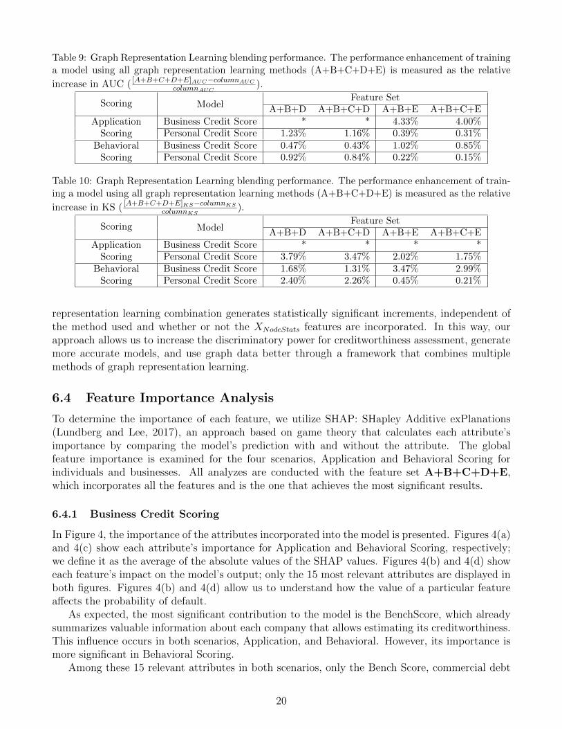
Table 9: Graph Representation Learning blending performance. The performance enhancement of traininga model using all graph representation learning methods (A+B+C+D+E) is measured as the relative
increase in AUC ( [A+B+C+D+E]AUC−columnAUC
columnAUC).
Scoring ModelFeature Set
A+B+D A+B+C+D A+B+E A+B+C+E
ApplicationScoring
Business Credit Score * * 4.33% 4.00%Personal Credit Score 1.23% 1.16% 0.39% 0.31%
BehavioralScoring
Business Credit Score 0.47% 0.43% 1.02% 0.85%Personal Credit Score 0.92% 0.84% 0.22% 0.15%
Table 10: Graph Representation Learning blending performance. The performance enhancement of train-ing a model using all graph representation learning methods (A+B+C+D+E) is measured as the relative
increase in KS ( [A+B+C+D+E]KS−columnKS
columnKS).
Scoring ModelFeature Set
A+B+D A+B+C+D A+B+E A+B+C+E
ApplicationScoring
Business Credit Score * * * *Personal Credit Score 3.79% 3.47% 2.02% 1.75%
BehavioralScoring
Business Credit Score 1.68% 1.31% 3.47% 2.99%Personal Credit Score 2.40% 2.26% 0.45% 0.21%
representation learning combination generates statistically significant increments, independent ofthe method used and whether or not the XNodeStats features are incorporated. In this way, ourapproach allows us to increase the discriminatory power for creditworthiness assessment, generatemore accurate models, and use graph data better through a framework that combines multiplemethods of graph representation learning.
6.4 Feature Importance Analysis
To determine the importance of each feature, we utilize SHAP: SHapley Additive exPlanations(Lundberg and Lee, 2017), an approach based on game theory that calculates each attribute’simportance by comparing the model’s prediction with and without the attribute. The globalfeature importance is examined for the four scenarios, Application and Behavioral Scoring forindividuals and businesses. All analyzes are conducted with the feature set A+B+C+D+E,which incorporates all the features and is the one that achieves the most significant results.
6.4.1 Business Credit Scoring
In Figure 4, the importance of the attributes incorporated into the model is presented. Figures 4(a)and 4(c) show each attribute’s importance for Application and Behavioral Scoring, respectively;we define it as the average of the absolute values of the SHAP values. Figures 4(b) and 4(d) showeach feature’s impact on the model’s output; only the 15 most relevant attributes are displayed inboth figures. Figures 4(b) and 4(d) allow us to understand how the value of a particular featureaffects the probability of default.
As expected, the most significant contribution to the model is the BenchScore, which alreadysummarizes valuable information about each company that allows estimating its creditworthiness.This influence occurs in both scenarios, Application, and Behavioral. However, its importance ismore significant in Behavioral Scoring.
Among these 15 relevant attributes in both scenarios, only the Bench Score, commercial debt
20
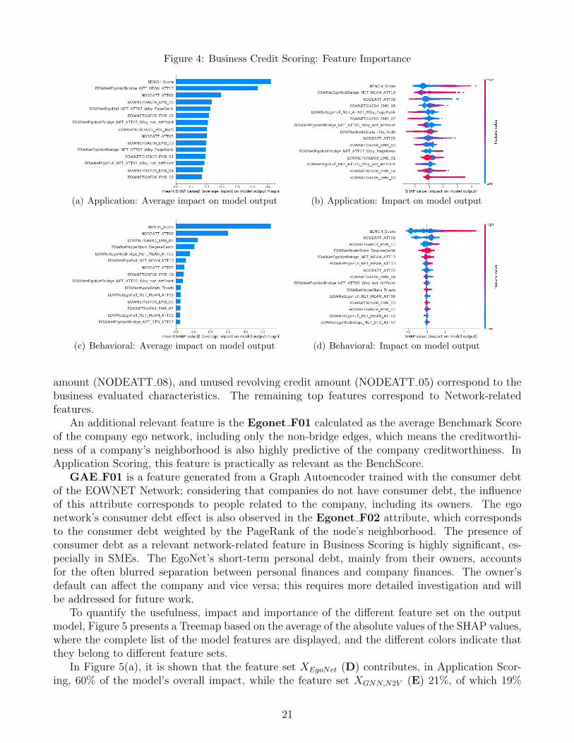
Figure 4: Business Credit Scoring: Feature Importance
(a) Application: Average impact on model output (b) Application: Impact on model output
(c) Behavioral: Average impact on model output (d) Behavioral: Impact on model output
amount (NODEATT 08), and unused revolving credit amount (NODEATT 05) correspond to thebusiness evaluated characteristics. The remaining top features correspond to Network-relatedfeatures.
An additional relevant feature is the Egonet F01 calculated as the average Benchmark Scoreof the company ego network, including only the non-bridge edges, which means the creditworthi-ness of a company’s neighborhood is also highly predictive of the company creditworthiness. InApplication Scoring, this feature is practically as relevant as the BenchScore.
GAE F01 is a feature generated from a Graph Autoencoder trained with the consumer debtof the EOWNET Network; considering that companies do not have consumer debt, the influenceof this attribute corresponds to people related to the company, including its owners. The egonetwork’s consumer debt effect is also observed in the Egonet F02 attribute, which correspondsto the consumer debt weighted by the PageRank of the node’s neighborhood. The presence ofconsumer debt as a relevant network-related feature in Business Scoring is highly significant, es-pecially in SMEs. The EgoNet’s short-term personal debt, mainly from their owners, accountsfor the often blurred separation between personal finances and company finances. The owner’sdefault can affect the company and vice versa; this requires more detailed investigation and willbe addressed for future work.
To quantify the usefulness, impact and importance of the different feature set on the outputmodel, Figure 5 presents a Treemap based on the average of the absolute values of the SHAP values,where the complete list of the model features are displayed, and the different colors indicate thatthey belong to different feature sets.
In Figure 5(a), it is shown that the feature set XEgoNet (D) contributes, in Application Scor-ing, 60% of the model’s overall impact, while the feature set XGNN,N2V (E) 21%, of which 19%
21

Figure 5: Business Credit Scoring: Treemap of Feature Importance, the average impact on model output
(a) Application Scoring
(b) Behavioral Scoring
correspond to GNN features, while 2% correspond to Node2Vec. This is likely the reason for thelimited research on Node2Vec to enhance the prediction of creditworthiness.
However, in Behavioral Business Scoring the traditional characteristics now represent 48 % ofthe total impact of the model. In contrast, for Business Application Scoring, only 16% (See Figure5(b)). Indeed, only the Bench Score attribute represented 29% of the total impact. The featureset XEgoNet (D) represents 30% of the total impact, the average BenchScore of the ego networkbeing the most relevant attribute.
6.4.2 Personal Credit Scoring
In Personal Scoring, the person’s characteristics (XNode +XBenchScore) produce a more meaningfulimpact than the business score. The person’s attributes represent 37% and 47% of the total impactfor Application and Behavioral Scoring, respectively.
Besides the BenchScore, other relevant features are consumer debt amount (NODEATT 07)and unused revolving credit amount, and total debt amount (NODEATT 01) (See Figures 6(a)and 6(c)).
The combined network features also play an essential role in the final score; the feature setXEgoNet (D) and XGNN,N2V (E) represent 25% and 33.4% in Application Scoring (See Figure7(a)), while the impact in Behavioral Scoring (See Figure 7(b)) are 18% and 28.3% respectively.In both cases, the contribution of Node2Vec features are negligible. The network feature with thehighest impact is the unused revolving credit amount of the network, as the average neighborhood’samount (Egonet F03).
Personal Credit Scoring included attributes generated with both FamilyNet and EOWNet net-works. When analyzing the network-related features, almost all of them in both scenarios are
22

Figure 6: Personal Credit Scoring: Feature Importance
(a) Application: Average impact on model output (b) Application: Impact on model output
(c) Behavioral: Average impact on model output (d) Behavioral: Impact on model output
FamilyNet features. These results show us the suitability of the network used to characterize bor-rowers and the importance of the type of relationship used to build the network. In this study,family ties were the most appropriate to characterize borrowers in the individual credit scoringproblem.
7 Conclusions
This study presents a methodology that allows us to assess the value delivered by complex graphdata to the credit scoring problem. This framework is applied in four scenarios, Application, andBehavioral Scoring, for individual and business lending. Additionally, this methodology allowsus to evaluate different Graph Representation Learning approaches to extract information fromnetworks: hand-crafted feature engineering, Node2Vec, and Graph Neural Networks. The resultsshow an improvement in creditworthiness assessment performance when different Graph Repre-sentation Learning approaches are combined. Specifically, two of the three Graph RepresentationLearning methods complement credit scoring models; these two methods are the Hand-craftedFeature Engineering and Graph Neural Networks and add the most value when used together. Webelieve this to be very relevant to the community as, until now, these two methods have been usedindependently. At the same time, the contribution of Node2Vec is negligible. This is likely thereason for the limited research on Node2Vec as a feature engineering method for credit scoring.
As a baseline, we use a credit scoring model developed by a financial institution. This modelalready outperforms bureau models, and our methodology allows us to obtain better results ineach of four scenarios.
23

Figure 7: Personal Credit Scoring: Treemap of Feature Importance, the average impact on model output
(a) Application Scoring
(b) Behavioral Scoring
The highest value is found in the Unbanked Application Scoring because applicants, individu-als, and companies, lack behavioral information, which turns out to be one of the best predictors ofcreditworthiness. In the case of the behavior scoring models, our methodology also improves per-formance. In both cases, the maximum performance is achieved when these Graph RepresentationLearning methods are used together.
Interpretability measures, such as SHAP values, allow us to understand each attribute’s con-tribution. Under this way of measuring the impact on the output model, the baseline model(BenchScore), although it continues to be an essential attribute, has diminished its effect as it isin the presence of other good predictors. This feature importance analysis allows us to understandthat we cannot solely examine its characteristics to evaluate a company, especially an unbankedone. We also have to understand that they are part of an ecosystem, where the owners, suppliers,clients, and related companies are essential. Their information allows us to improve the creditwor-thiness assessment performance. A similar situation occurs in Personal Credit Scoring, althoughwith less intensity. The network data allows us to address the scarcity of information and achievea better credit risk assessment.
Our research tells us that there is still room for improvement in incorporating network infor-mation into the credit scoring problem. This methodology goes in the right direction, improvingcreditworthiness assessment performance. It has great value for the unbanked and under-bankedpeople and even in the portfolio’s credit risk management.
Acknowledgments
This work would not have been accomplished without the financial support of CONICYT-PFCHA/ DOCTORADO BECAS CHILE / 2019-21190345. The second author acknowledges the supportof the Natural Sciences and Engineering Research Council of Canada (NSERC) [Discovery Grant
24

RGPIN-2020-07114]. This research was undertaken, in part, thanks to funding from the CanadaResearch Chairs program. The last author thanks the partial support of FEDER funds throughthe MINECO project TIN2017-85827-P and the European Union’s Horizon 2020 research andinnovation program under the Marie Sklodowska-Curie grant agreement No 777720.
References
Akoglu, H. (2018). User’s guide to correlation coefficients. Turkish Journal of Emergency Medicine,18.
Apostolik, R., Donohue, C., and Went, P. (2009). Foundations of banking risk: an overview ofbanking, banking risks, and risk-based banking regulation, volume 507. John Wiley & SonsIncorporated.
Arsov, N. and Mirceva, G. (2019). Network embedding: An overview. arXiv preprintarXiv:1911.11726.
Aziz, S. and Dowling, M. (2019). Machine Learning and AI for Risk Management, pages 33–50.Springer International Publishing, Cham.
Baidoo, E. (2020). A credit analysis of the unbanked and underbanked: an argument for alternativedata. PhD dissertation, Analytics and Data Science Institute, Kennesaw State University.
Bradley, A. P. (1997). The use of the area under the roc curve in the evaluation of machine learningalgorithms. Pattern recognition, 30(7):1145–1159.
Bravo, C., Thomas, L. C., and Weber, R. (2015). Improving credit scoring by differentiatingdefaulter behaviour. The Journal of the Operational Research Society, 66(5):771–781.
Bravo, C. and Oskarsdottir, M. (2020). Evolution of credit risk using a personalized pagerankalgorithm for multilayer networks. arXiv preprint arXiv:2005.12418.
Breiman, L. (2001). Random forests. Machine learning, 45(1):5–32.Cnudde, S. D., Moeyersoms, J., Stankova, M., Tobback, E., Javaly, V., and Martens, D. (2019).
What does your facebook profile reveal about your creditworthiness? using alternative datafor microfinance. Journal of the Operational Research Society, 70(3):353–363.
Cusmano, L. (2018). SME and entrepreneurship financing: The role of credit guarantee schemesand mutual guarantee societies in supporting finance for small and medium-sized enterprises.OECD SME and Entrepreneurship Papers, No. 1.
Defferrard, M., Bresson, X., and Vandergheynst, P. (2016). Convolutional neural networks ongraphs with fast localized spectral filtering. In Advances in neural information processingsystems, pages 3844–3852.
Diallo, B. and Al-Titi, O. (2017). Local growth and access to credit: Theory and evidence. Journalof Macroeconomics, 54:410–423. Banking in Macroeconomic Theory and Policy.
Djeundje, V. B., Crook, J., Calabrese, R., and Hamid, M. (2021). Enhancing credit scoring withalternative data. Expert Systems with Applications, 163:113766.
Easley, D. and Kleinberg, J. (2010). Networks, Crowds, and Markets: Reasoning About a HighlyConnected World. Cambridge University Press, USA.
Fey, M. and Lenssen, J. E. (2019). Fast graph representation learning with pytorch geometric.arXiv preprint arXiv:1903.02428.
Flach, P. A. (2012). Machine Learning - The Art and Science of Algorithms that Make Sense ofData. Cambridge University Press.
Freedman, S. and Jin, G. Z. (2017). The information value of online social networks: Lessons frompeer-to-peer lending. International Journal of Industrial Organization, 51:185 – 222.
25

Friedman, J. H. (2001). Greedy function approximation: a gradient boosting machine. Annals ofstatistics, pages 1189–1232.
Grover, A. and Leskovec, J. (2016). Node2vec: Scalable feature learning for networks. In Pro-ceedings of the 22nd ACM SIGKDD International Conference on Knowledge Discovery andData Mining, KDD ’16, page 855–864, New York, NY, USA. Association for ComputingMachinery.
Hagberg, A., Swart, P., and SChult, D. (2008). Exploring network structure, dynamics, andfunction using networkx. In In Proceedings of the 7th Python in Science Conference (SciPy,pages 11–15. Citeseer.
Hamilton, W. L., Ying, R., and Leskovec, J. (2017). Representation learning on graphs: Methodsand applications. arXiv preprint arXiv:1709.05584.
Hodges, J. (1958). The significance probability of the smirnov two-sample test. Arkiv for Matem-atik, 3(5):469–486.
Hurley, M. and Adebayo, J. (2017). Credit scoring in the era of big data. Yale Journal of Law andTechnology, 18(1):5.
Kaufman, S., Rosset, S., Perlich, C., and Stitelman, O. (2012). Leakage in data mining: Formula-tion, detection, and avoidance. ACM Trans. Knowl. Discov. Data, 6(4).
Kipf, T. N. and Welling, M. (2016a). Semi-supervised classification with graph convolutionalnetworks. arXiv preprint arXiv:1609.02907.
Kipf, T. N. and Welling, M. (2016b). Variational graph auto-encoders. arXiv preprintarXiv:1611.07308.
Kleinberg, J. M. (1999). Authoritative sources in a hyperlinked environment. J. ACM,46(5):604–632.
Leskovec, J. and Sosic, R. (2016). Snap: A general-purpose network analysis and graph-mininglibrary. ACM Transactions on Intelligent Systems and Technology (TIST), 8(1):1.
Lessmann, S., Baesens, B., Seow, H.-V., and Thomas, L. C. (2015). Benchmarking state-of-the-art classification algorithms for credit scoring: An update of research. European Journal ofOperational Research, 247(1):124–136.
Lin, M., Prabhala, N. R., and Viswanathan, S. (2013). Judging borrowers by the company theykeep: Friendship networks and information asymmetry in online peer-to-peer lending. Man-agement Science, 59(1):17–35.
Lundberg, S. M. and Lee, S.-I. (2017). A unified approach to interpreting model predictions. InProceedings of the 31st international conference on neural information processing systems,pages 4765–4774, Red Hook, NY, USA. Curran Associates Inc.
Maldonado, S., Perez, J., and Bravo, C. (2017). Cost-based feature selection for support vectormachines: An application in credit scoring. European Journal of Operational Research,261(2):656 – 665.
Masyutin, A. (2015). Credit scoring based on social network data. Business Informatics, 3(33):15–23.
Nargesian, F., Samulowitz, H., Khurana, U., Khalil, E. B., and Turaga, D. (2017). Learningfeature engineering for classification. In Proceedings of the Twenty-Sixth International JointConference on Artificial Intelligence, IJCAI-17, pages 2529–2535.
Okten, C. and Osili, U. O. (2004). Social networks and credit access in indonesia. World Devel-opment, 32(7):1225 – 1246.
Oskarsdottir, M., Bravo, C., Vanathien, J., and Baesens, B. (2018a). Credit scoring for good:enhancing financial inclusion with smartphone-based microlending. In Proceedings of theThirty Ninth International Conference on Information Systems, San Francisco, California,
26

USA.Oskarsdottir, M., Bravo, C., Vanathien, J., and Baesens, B. (2018b). Social network analytics in
micro-lending. In 29th European Conference on Operational Research (08/07/18 - 11/07/18),Valencia, Spain.
Oskarsdottir, M. and Bravo, C. (2021). Multilayer network analysis for improved credit riskprediction. Omega, 105:102520.
Oskarsdottir, M., Bravo, C., Sarraute, C., Vanthienen, J., and Baesens, B. (2019). The value ofbig data for credit scoring: Enhancing financial inclusion using mobile phone data and socialnetwork analytics. Applied Soft Computing, 74:26 – 39.
Oskarsdottir, M., Bravo, C., Verbeke, W., Baesens, B., and Vanthienen, J. (2018). Effects ofnetwork architecture on model performance when predicting churn in telco.
Oskarsdottir, M., Bravo, C., Verbeke, W., Sarraute, C., Baesens, B., and Vanthienen, J. (2016). Acomparative study of social network classifiers for predicting churn in the telecommunicationindustry. In 2016 IEEE/ACM International Conference on Advances in Social NetworksAnalysis and Mining (ASONAM), pages 1151–1158.
Oskarsdottir, M., Bravo, C., Verbeke, W., Sarraute, C., Baesens, B., and Vanthienen, J. (2017).Social network analytics for churn prediction in telco: Model building, evaluation and networkarchitecture. Expert Systems with Applications, 85:204 – 220.
Paszke, A., Gross, S., Massa, F., Lerer, A., Bradbury, J., Chanan, G., Killeen, T., Lin, Z.,Gimelshein, N., Antiga, L., et al. (2019). Pytorch: An imperative style, high-performancedeep learning library. Advances in neural information processing systems, 32:8026–8037.
Putra, S. G. P., Joshi, B., Redi, J., and Bozzon, A. (2020). A credit scoring model for smesbased on social media data. In Bielikova, M., Mikkonen, T., and Pautasso, C., editors, WebEngineering, pages 113–129, Cham. Springer International Publishing.
Rabecca, H., Atmaja, N. D., and Safitri, S. (2018). Psychometric credit scoring in indonesia mi-crofinance industry: A case study in pt amartha mikro fintek. In The 3rd InternationalConference on Management in Emerging Markets (ICMEM 2018), pages 620–631, Bali, In-donesia.
Roa, L., Correa-Bahnsen, A., Suarez, G., Cortes-Tejada, F., Luque, M. A., and Bravo, C. (2021a).Super-app behavioral patterns in credit risk models: Financial, statistical and regulatoryimplications. Expert Systems with Applications, 169:114486.
Roa, L., Rodrıguez-Rey, A., Correa-Bahnsen, A., and Valencia, C. (2021b). Supporting financialinclusion with graph machine learning and super-app alternative data.
Ruiz, S., Gomes, P., Rodrigues, L., and Gama, J. (2017). Credit scoring in microfinance usingnon-traditional data. In Oliveira, E., Gama, J., Vale, Z., and Lopes Cardoso, H., editors,Progress in Artificial Intelligence, pages 447–458, Cham. Springer International Publishing.
Shoham, D. (2004). Psychometric creditworthiness scoring for business loans. US Patent App.10/708,427.
Shumovskaia, V., Fedyanin, K., Sukharev, I., Berestnev, D., and Panov, M. (2020). Linking bankclients using graph neural networks powered by rich transactional data.
Silver, L. (2001). Credit risk assessment in different contexts : The influence of local networks forbank financing of SMEs. PhD thesis, Uppsala University, Department of Business Studies.
Stevenson, M., Mues, C., and Bravo, C. (2021). The value of text for small business default predic-tion: A deep learning approach. European Journal of Operational Research, 295(2):758–771.
Sukharev, I., Shumovskaia, V., Fedyanin, K., Panov, M., and Berestnev, D. (2020). Ews-gcn: Edgeweight-shared graph convolutional network for transactional banking data.
The Basel Committee on Banking Supervision (2000). Principles for the management of credit
27

risk. Basel Committee Publications, 75.The Global Financial Index (2017). The unbanked. https://globalfindex.worldbank.org/
chapters/unbanked (Accessed November, 2020).Thomas, L., Crook, J., and Edelman, D. (2017). Credit scoring and its applications. SIAM.Vlasselaer, V. V., Bravo, C., Caelen, O., Eliassi-Rad, T., Akoglu, L., Snoeck, M., and Baesens,
B. (2015). Apate: A novel approach for automated credit card transaction fraud detectionusing network-based extensions. Decision Support Systems, 75:38 – 48.
Verbraken, T., Bravo, C., Weber, R., and Baesens, B. (2014). Development and application ofconsumer credit scoring models using profit-based classification measures. European Journalof Operational Research, 238(2):505 – 513.
Wei, Y., Yildirim, P., Van den Bulte, C., and Dellarocas, C. (2016). Credit scoring with socialnetwork data. Marketing Science, 35(2):234–258.
Wu, Z., Pan, S., Chen, F., Long, G., Zhang, C., and Yu, P. S. (2020). A comprehensive surveyon graph neural networks. IEEE Transactions on Neural Networks and Learning Systems,pages 1–21.
Zhang, M. and Chen, Y. (2018). Link prediction based on graph neural networks. In Advances inNeural Information Processing Systems, pages 5165–5175.
28