On the Common Ancestors of All Living Humans

Douglas L. T. RohdeMassachusetts Institute of Technology

November 11, 2003

AbstractQuestions concerning the common ancestors of allpresent-day humans have received considerable attentionof late in both the scientific and lay communities. Princi-pally, this attention has focused on ‘Mitochondrial Eve,’defined to be the woman who lies at the confluence of ourmaternal ancestry lines, and who is believed to have lived100,000–200,000 years ago. More recent attention hasbeen given to our common paternal ancestor, ‘Y Chromo-some Adam,’ who may have lived 35,000–89,000 yearsago. However, if we consider not just our all-female andall-male lines, but our ancestors along all parental lines,it turns out that everyone on earth may share a commonancestor who is remarkably recent.

This study introduces a large-scale, detailed computermodel of recent human history which suggests that thecommon ancestor of everyone alive today very likely livedbetween 2,000 and 5,000 years ago. Furthermore, themodel indicates that nearly everyone living a few thou-sand years prior to that time is either the ancestor of noone or of all living humans.

1 IntroductionAdvances in genetics have sparked interest in our com-mon ancestors, the individuals from which all present-dayhumans descend. Initial interest focused on the topic of‘Mitochondrial Eve,’ who is defined to be the most re-cent female ancestor from whom all individuals descendalong strictly maternal lines (Cann, Stoneking, & Wilson,1987; Vigilant, Stoneking, Harpending, Hawkes, & Wil-son, 1991). An approximate date for Mitochondrial Eveof 100,000 to 200,000 years ago has been estimated basedon the successive mutations in mitochondrial DNA, whichare passed down from mother to child. A similar analy-sis can be performed on the strictly paternal lines of suc-cession, using the Y chromosome, which is passed downfrom father to son, to determine the approximate date of‘Y Chromosome Adam.’ This date was originally esti-mated very loosely to fall between 27,000 and 270,000

∗Work in progress. Do not cite.

years ago (Dorit, Akashi, & Gilbert, 1995), a range thatwas more recently narrowed to 35,000–89,000 years ago(Ke et al., 2001).

Nevertheless, an individual’s strictly maternal andstrictly paternal lines are just two of a vast number of pos-sible paths back through his or her ancestors. What if weadopt a more common-sense notion of ancestry that in-cludes ancestors reachable along any path of succession,using both mothers and fathers? It seems likely that ourmost recent common ancestor (MRCA) under this broaderdefinition will be much more recent than either Mitochon-drial Eve or Y Chromosome Adam. Unfortunately, theage of our MRCA cannot as easily be estimated on thebasis of genetic information because the relevant genesare not passed from parent to child with only occasionalmutations but are, rather, the product of recombination.As a result of recombination, a given gene may not passfrom parent to child. In fact, an individual’s DNA mayretain none of the genes specific to a particular ancestorwho lived many generations in the past. These additionalcomplications make accurately dating the MRCA or re-constructing other details of population history on the ba-sis of our genes extremely difficult, if not impossible (Hey& Machado, 2003).

However, alternative methods may be able to answerthis question. Some researchers have produced estimatesof the age of our MRCA by means of the theoreticalanalysis of mathematical models. Building on work byKammerle (1991) and Mohle (1994), Chang (1999) ana-lyzed a model that assumes a fixed-size population, withdiscrete and non-overlapping generations, and randommating. That is, each child is the product of two parents,randomly selected from all members of the previous gen-eration. Chang showed that, in this model, the mixing ofgenes occurs quite rapidly. In fact, the number of gener-ations back to the MRCA is expected to be about log2 ofthe population size. With a population of 6 billion people,this model predicts that the MRCA is likely to occur injust over 32 generations, or 800–975 years. This suggeststhat our all-paths MRCA may be exceptionally recent.

But Chang was well aware of the limitations of thesimple model he analyzed. “What are the significance

ROHDE COMMON ANCESTORS OF ALL LIVING HUMANS

of these results? An application to the world populationof humans would be an obvious misuse. . . An importantsource of inapplicability of the model to this situation isthe obvious non-random nature of mating in the history ofmankind.” (pg. 1005) There are many factors that limitthe randomness of human mating. First of all, clearly, aresex differences, but Chang did address this, noting thatadding distinct sexes to the model would not cause a sub-stantial change in the estimate. Another factor is mar-riage. Once a couple has one child, they are likely to re-main together as they produce more children. Moreover,broader sociological and geographic factors may have stillmore profound effects. In short, although we are becom-ing increasingly panmictic, humans groups have tendedtowards a high rate of endogamy, finding mates almostexclusively within the local population and social class,only occasionally transcending barriers of geography, lan-guage, race, and culture.

It seems likely that these restrictions on the random-ness of human mating may dramatically decrease the rateof ancestral mixing in the model. As a result, the true dateof the MRCA could be thousands or tens of thousands ofyears ago, rather than just hundreds. Thus, an obviousnext step is to test this possibility by expanding the modelto include some or all of these constraints. Unfortunately,conducting a theoretical analysis of a more complicatedmathematical model would be very difficult. An alterna-tive approach is to implement a computer simulation. Theprincipal advantage of a computer simulation is that it canbe arbitrarily complex. However, even given the speed oftoday’s computer, efficiently simulating the ancestral his-tory of a population whose size is even close to the scaleof humanity is non-trivial. Furthermore, because a non-random model will necessarily involve numerous param-eters that cannot be adequately constrained by availabledata, the simulation must typically be run many times toexplore the consequences of various parameter settings.

This study involves the implementation and analysis ofseveral large-scale computer models of recent human his-tory. The models simulate individual human lives, includ-ing life span, birth rate, choice of mates, and migration,and the data they produce is analyzed to obtain more ac-curate estimates of the date of our most recent commonancestor. Given what seem to be reasonable parameterchoices, the final, most detailed model presented here pre-dicts that our most recent common ancestor probably livedbetween 2000 and 5000 years ago and that nearly every-one alive prior to a few thousand years before that are theancestors of either no one or of everyone alive today.

1.1 Modeling human genealogy

Mathematical models of human genealogy must be quitesimple if their analysis is to be possible. Most, like

Chang’s, are some variant of a Wright-Fisher model, withdiscrete generations and parents selected at random fromthe preceding generation (Nordborg, 2001). Becausecomputer simulations are tested empirically rather thanthrough theoretical analysis, they are not subject to suchconstraints.

However, there are practical limits to the complexityof a computer simulation. One is the matter of computa-tional efficiency. A model cannot be so complex that run-ning it requires an unreasonable amount of time or space.A more significant limitation, from a scientific perspec-tive, must be placed on the number of free parameters inthe model. Ideally, for the results of a model to be reli-able, any free parameters should be constrained by his-torical data, such as statistics on actual birth or migrationrates. However, much of the relevant data for the currentmodels concern events occurring thousands of years agoand cannot be obtained with any accuracy. In this case,the parameters must be varied within the range of plau-sible values to obtain bounds on the model’s predictions.A model with too many free parameters, especially onesunconstrained by empirical data, will have reduced powerand will be difficult to study. Therefore, a good modelmust be complex enough to include relevant factors, butnot overly burdened by irrelevant ones.

This study explores a progression of three models. Thefirst extends Chang’s results to a world consisting of fivemore or less panmictic islands, or continents, with onlyoccasional migrants between any pair of continents. Thesecond model, discussed in Section 3 arranges the islandsin a graph that roughly reflects the topology of the ma-jor world continents. The final model, discussed in Sec-tion 4, is a more detailed simulation of the actual world,with migration routes and dates based on historical dataor prehistoric estimates.

2 Model A: Fully-connectedcontinents

The first model, A, is quite abstract but incorporates sev-eral levels of detail beyond those found in most Wright-Fisher models. The model typically starts between 5000and 20000 BC and runs to the present day, which is takento be the year 2000 AD. As the model runs, it simu-lates important details in the lives of individual people,known as sims, including their lifespans, possible migra-tions, choice of mate, and production of offspring. Asthe model runs, it records this information in a series oflarge computer files. A second program, discussed in Sec-tion 2.2, traces ancestral lines through this data to find thecommon ancestors.

2

ROHDE COMMON ANCESTORS OF ALL LIVING HUMANS

2.1 Details of the model2.1.1 Life span

The present models do not assume discrete, uniform gen-erations. Each sim is born in a certain year and has aparticular life span. The maximum age of any sim wasset to 100, as it seems highly unlikely that anyone wouldlive, let alone father children, beyond that age. The ageof sexual maturity was taken to be 16 years for both menand women. Anyone who would have died before that agecould not have produced offspring and is thus not a factorfor the purposes of this study. Therefore, only the lives ofthose destined to at least reach adulthood were simulated.As a result, the population sizes discussed throughout thispaper are effectively somewhat larger than stated becausethey do not include any children.

Otherwise, the probability that an individual dies at ages, conditional on not having died before age s, is assumedto follow a discrete Gompertz-Makeham form (Pletcher,1999):

p(s) = α + (1 − α)e(s−100)/β

In this equation, β is the death rate. A higher death rateresults in shorter life spans on average, although the resultis not linear. The α parameter is the accident rate, whichcan be adjusted to reflect the probability that an individ-ual of any age dies of unnatural causes. With an accidentrate of 0.01 and a death rate of 10.5, this formula quiteclosely models the life span data for the U.S. between1900 and 1930 (U.S. National Office of Vital Statistics,1956). To account for historically shorter life spans dueto poor nutrition, medicine, and so forth, the death rate,β, was raised to 12.5 for the purposes of the model. Thisproduces an average life span of 51.8 for those who reachmaturity.

The percentage of males born into the population wasset at 50%. It is true that the actual percentage of malesand females reaching adulthood may differ somewhat dueto infanticide coupled with the fact that a slightly higherpercentage of newborns are male than female (Davis, Got-tlieb, & Stampnitzky, 1998). But this probably does nothave much bearing on the results of the model. And whileit is true that women tend to live longer, the life span ofwomen past child-bearing age is also not relevant to theoutcome of the model. Therefore, for simplicity, the lifespans of males and females were generated using the samedistribution.

2.1.2 Migration

The models are organized into three structural levels: con-tinents, countries, and towns. The continents representphysically separated land masses that are likely to havevery low rates of inter-migration. Europe and Asia are

contiguous, with no substantial geographical barrier tomigration, so they will be considered a single continent,along with Africa, North America, and South America.Indonesia, Australia, and Oceania are, taken together,somewhat more difficult to model, as there is clearly sub-stantial internal structure. For the purposes of the first twomodels, they will be considered a single continent, butwill be dealt with more appropriately in the third model.

The models’ continents are divided into countries, ar-ranged in a grid. These reflect major tribal, ethnic, orlanguage groups, with both geographic and cultural bar-riers to intermarriage. Countries are, in turn, divided intotowns. These do not necessarily represent towns per se,but the relevant social unit from within which most peo-ple find mates. Thus, a town may actually reflect a clan,a rural county, or even a particular social class within alarger group. The towns within each country are assumedto be in relatively frequent contact with one another andare not in any particular geographic arrangement.

Not all humans confine themselves to a single locationthroughout their lives and a critical factor in the model isthe rate at which people migrate to different places in theworld. Although it seems likely that many people, andperhaps the vast majority historically, live out their livesclose to where they were born, various forms of migrationlead to the gradual spread of ancestral lineages over longdistances. When men and women from different groupsmarry, one of them, often the wife but sometimes the hus-band, moves to the other’s community. Merchants, sol-diers, and bureaucrats, who are typically male, sometimestravel widely, potentially fathering children far from theirplace of birth. And, occasionally, large groups of peoplehave conquered or colonized new areas.

In terms of realism, it would certainly be desirable todistinguish between these and other specific types of mi-gration in the model. However, doing so would introducemany new parameters, for which we are unlikely to findsufficient data. Therefore, the model uses a simplified mi-gration system, in which each person can move only oncein his or her life. Each sim is born in the town in whichhis or her parents, or at least mother, lives, but then hasa chance to migrate to a different continent, country, ortown prior to adulthood. Henceforth, that person can pro-duce children only with other inhabitants of his or her newtown, provided it contains potential mates.

As is the case in human mating patterns (Fix, 1979),the rate of exogamy decreases substantially with largergroup size in the models. Adams and Kasakoff (1976)found that, across a variety of human societies, there wasa recognizable threshold in group size at around a 20%exogamy rate, although the sizes of these groups differedas a function of population density. This “natural” groupsize is taken here to be that of the town. The Change-TownProb parameter controls the percentage of sims who

3

ROHDE COMMON ANCESTORS OF ALL LIVING HUMANS

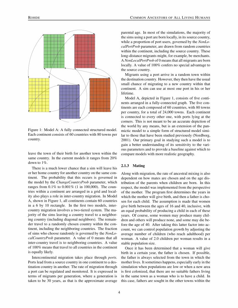
Figure 1: Model A: A fully connected structured model.Each continent consists of 60 countries with 80 towns percountry.

leave the town of their birth for another town within thesame country. In the current models it ranges from 20%down to 1%.

There is a much lower chance that a sim will leave hisor her home country for another country on the same con-tinent. The probability that this occurs is governed inthe model by the ChangeCountryProb parameter, whichranges from 0.1% to 0.001% (1 in 100,000). The coun-tries within a continent are arranged in a grid and local-ity also plays a role in inter-country migration. In ModelA, shown in Figure 1, all continents contain 60 countriesin a 6 by 10 rectangle. In the first two models, inter-country migration involves a two-tiered system. The ma-jority of the sims leaving a country travel to a neighbor-ing country (including diagonal neighbors). The remain-der travel to a randomly chosen country within the con-tinent, including the neighboring countries. The fractionof sims who choose randomly is governed by the NonLo-calCountryProb parameter. A value of 0 means that allinter-country travel is to neighboring countries. A valueof 100% means that travel to all countries in the continentis equally likely.

Intercontinental migration takes place through ports.Ports lead from a source country in one continent to a des-tination country in another. The rate of migration througha port can be regulated and monitored. It is expressed interms of migrants per generation, where a generation istaken to be 30 years, as that is the approximate average

parental age. In most of the simulations, the majority ofthe sims using a port are born locally, in its source country,while a proportion of port users, governed by the NonLo-calPortProb parameter, are drawn from random countrieswithin the continent, including the source country. Theselong-distance migrants might, for example, be merchants.A NonLocalPortProb of 0 means that all migrants are bornlocally. A value of 100% confers no special advantage tothe source country.

Migrants using a port arrive in a random town withinthe destination country. However, they then have the usualsmall chance of migrating to a new country within thatcontinent. A sim can use at most one port in his or herlifetime.

Model A, depicted in Figure 1, consists of five conti-nents arranged in a fully-connected graph. The five con-tinents are each composed of 60 countries, with 80 townsper country, for a total of 24,000 towns. Each continentis connected to every other one, with ports lying at thecorners. This is not meant to be an accurate depiction ofthe world by any means, but is an extension of the pan-mictic model to a simple form of structured model simi-lar to those that have been studied previously (Nordborg,2001). Our primary goal in studying such a model is togain a better understanding of its sensitivity to the vari-ous parameters and to provide a baseline against which tocompare models with more realistic geography.

2.1.3 Mating

Along with migration, the rate of ancestral mixing is alsodependent on how mates are chosen and on the age dis-tribution of the parents when children are born. In thisrespect, the model was implemented from the perspectiveof the mother. The program first determines the years inwhich the mother will give birth, and then a father is cho-sen for each child. The assumption is made that womengive birth between the ages of 16 and 40, inclusive, withan equal probability of producing a child in each of theseyears. Of course, some women may produce many chil-dren and others will produce none, and some may die be-fore the age of 40. After taking this latter factor into ac-count, we can control population growth by adjusting theaverage number of children (who reach adulthood) perwoman. A value of 2.0 children per woman results in astable population size.

Once it has been determined that a woman will givebirth in a certain year, the father is chosen. If possible,the father is always selected from the town in which themother lives. It sometimes happens, especially early in thesimulation when populations are low or when a new areais first colonized, that there are no suitable fathers livingin the same town as a woman who is to have a child. Inthis case, fathers are sought in the other towns within the

4

ROHDE COMMON ANCESTORS OF ALL LIVING HUMANS

0 2 4 6 8 10 12 14Number of Children

0%

5%

10%

15%

20%

25%

30%

35%

Perc

enta

ge o

f Men

or W

omen

WomenMen (Models A and B)Men (Model C)

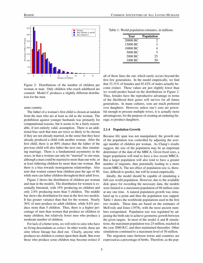
Figure 2: Distributions of the number of children perwoman or man. Only children who reach adulthood arecounted. Model C produces a slightly different distribu-tion for the men.

same country.The father of a woman’s first child is chosen at random

from the men who are at least as old as the woman. Theprohibition against younger husbands was primarily forcomputational reasons, but it seems to be a fairly reason-able, if not entirely valid, assumption. There is an addi-tional bias such that men are twice as likely to be chosenif they are not already married, in the sense that they havealready produced a child with another woman. After thefirst child, there is an 80% chance that the father of theprevious child will also father the next one, thus simulat-ing marriage. There is a fundamental asymmetry in thesexes, in that a woman can only be “married” to one man,although a man could be married to more than one wife, orat least fathering children by more than one woman. Butthere is a bias towards monogamous relationships. Alsonote that women cannot bear children past the age of 40,while men can father children throughout their adult lives.

Figure 2 shows the distribution of children per womanand man in the models. The distribution for women is es-sentially binomial, with 19% producing no children andonly 2.8% producing more than 5 children. The middlebar shows the distribution for men in the first two models.It has greater variance than that for the women. Nearly36% of men produce no adult children, while 8.6% pro-duce more than 5 children. Thus, there is a higher per-centage of men than women that produce no children ormany children, but relatively fewer men who produce amoderate number of children.

For lack of a better term, we will refer to sims who haveno living descendants as extinct. In other words, these aresims whose lineage has died out. Clearly, anyone whoproduces no children is extinct upon their death. But eventhose who produce some children may become extinct if

Table 1: World population estimates, in millions.

Year Population20000 BC 215000 BC 310000 BC 4

5000 BC 52000 BC 251000 BC 50

all of those lines die out, which rarely occurs beyond thefirst few generations. In the model empirically, we findthat 33.31% of females and 45.42% of males actually be-come extinct. These values are just slightly lower thanwe would predict based on the distributions in Figure 2.Thus, females have the reproductive advantage in termsof the likelihood their genes will survive for all futuregenerations. In many cultures, sons are much preferredover daughters. However, unless one’s sons are power-ful enough to procure multiple wives, it is actually moreadvantageous, for the purpose of creating an enduring lin-eage, to produce daughters.

2.1.4 Population Growth

Because life span was not manipulated, the growth rateof the population was controlled by adjusting the aver-age number of children per woman. As Chang’s resultssuggest, the size of the population may be an importantdeterminer of the date of the MRCA. Given fixed sizes, alarger population will tend to have a less recent MRCA.But a larger population will also tend to have a greaternumber of migrants, thus potentially leading to a morerecent MRCA. The net effect of population size is, there-fore, difficult to predict, but will be tested empirically.

Ideally, the model should be capable of simulating afull-size world population. However, due to the availabledisk space for recording the necessary data, the modelswere limited to a maximum population of 60 million simsat any one time. A natural population growth was simu-lated up to a point and then the population was capped.Table 1 shows the worldwide populations used in the firsttwo models. These data are based on the estimates ofMcEvedy and Jones (1978), with the most ancient num-bers extrapolated. Population size was regulated by ad-justing the birth rate to achieve geometric growth betweenthe given targets. In most of the model A and B simula-tions, the maximum population was 25 million, reached inthe year 2000 B.C, and then maintained thereafter. Othersimulations continued to a maximum level of 50 million.

The migration rates between towns and countries areexpressed as a percentage of births. Therefore, as the pop-

5

ROHDE COMMON ANCESTORS OF ALL LIVING HUMANS

ulation increases, the total number of migrants increasesproportionally. In Models A and B, the rate of the portswas fixed to achieve a particular number of migrants pergeneration once the population had reached maximumsize. However, prior to that point, proportionately fewermigrants would be using the ports.

2.1.5 Initialization

There is one remaining aspect of the model to be de-scribed, which is the method of initialization. Althoughsome simulations were started in the year 20000 BC, oth-ers were started as recently as 5000 BC if a more recentstart date would not interfere with the results. In orderto get things going, we need some initial sims. A sim-ple approach might be to create all of the initial sims inthe same year. However, in that case, their children wouldform a baby boom and it would take some time for the agedistribution within the population to stabilize. Unless thatstable age distribution is known in advance, there will al-ways be some instability introduced by the creation of theinitial people.

Therefore, the simulation actually begins 100 years be-fore the desired start date. An initial set of sims is gen-erated, each in a random town and each born at a randomtime within a 40-year window. The model is then run asusual, with the initial sims starting to produce offspring.Although the population does not have a natural age pro-file initially, as there are no old people, it quickly settlesinto a near-normal distribution within the first 100 years.The population will roughly double during these first 100years as fewer people die of old age than are born. Thus,the size of the initial population is adjusted to achieve thedesired level at the end of the 100-year period.

2.2 Finding common ancestors

A simulation with a maximum population of 50 millionsims will involve a total of approximately 1.2 billion simsover its course. As the model runs, it generates files con-taining the vital statistics of each sim, including his or herparents, sex, birth and death years, and place of birth, typ-ically totaling about 60 gigabytes of compressed data pertrial. Although running the simulation is relatively easy,analyzing this genealogical data to identify the commonancestors presents a significant computational problem.

Let us refer to all of the sims alive in the year 2000,when the simulations end, as living sims. A true com-mon ancestor (CA) is someone who is an ancestor of allliving sims. A straightforward search for common ances-tors would start with the living sims and work backwardsin time, tracking for every other sim, which of the livingsims are his or her descendants. These descendants arethe union of all descendants of his or her children. Track-

ing the descendants would be fairly simple, except that itrequires memory proportional to the square of the numberof living sims. With a maximum population of 50 mil-lion, this would involve the computation and storage ofover 300 terabytes of information.

Therefore, finding the common ancestors is nottractable using a straightforward approach. However, amethod was developed to zero in on the common ances-tors using an initial approximation followed by a seriesof refinements. This process begins by tracking the an-cestry not of all living sims, but of a small, randomly se-lected subset of them. Depending on the available com-puter memory, there are typically between 192 and 512 ofthese individuals, who are known as tracers. By workingbackwards through the records, the ancestry of these trac-ers is determined. This is done by computing, for everyother sim, a bit vector in which the ith bit is turned on ifthat sim is an ancestor of the ith tracer. Aside from the factthat the ith tracer automatically has the ith bit turned on,a parent’s bit vector will be the bit-wise disjunction of hisor her children’s vectors. These bit vectors still presenta heavy memory burden, but can be handled more effi-ciently by storing only the unique vectors.

If a sim is not an ancestor of every one of the tracers,that sim could not possibly be a common ancestor (CA).However, if a sim is a common ancestor of all of the trac-ers, there is a high probability that the sim is an ancestorof a large proportion of the living sims. Such ancestors arereferred to as potential common ancestors (PCAs). Unfor-tunately, it is generally the case that the most recent PCAsthat are found in this first backward phase are not actu-ally true CAs. Therefore, this superset of the CAs mustbe refined.

The next step is to start with a set of the most re-cent PCAs and trace their lineage forward through time.This is done in much the same way that descendancy wastraced in the backward phase—a sim’s ancestors are thedisjunction of his or her parents’ ancestors. In this case,we eventually determine which of the most recent PCAsis an ancestor of each of the living sims. If one of thePCAs was an ancestor of all of the living sims, then weare guaranteed to have found the true MRCA. Otherwise,a new set of tracers is chosen and a second backward passis performed to refine the set of PCAs.

Selecting the new set of tracers randomly would helpa little bit, but not much. A more effective approach isto try to find the sims who are difficult to reach, meaningthat they descend from the fewest number of the PCAs.We also need to find a diverse set of tracers. If they are alldifficult to reach because they live in the same place, theuse of more than one as a tracer would be redundant. Inorder to satisfy these constraints, the tracers are selectedin order, with the next tracer chosen being the living simwith the highest score, defined as follows:

6

ROHDE COMMON ANCESTORS OF ALL LIVING HUMANS

scorei =∑

p∈P

2−

(

xp,i+∑

t∈Txp,t

)

In this equation, i is the sim being considered as a pos-sible tracer. P is the set of PCAs whose descendants weretracked. The indicator variable xp,i is 1 if sim i is not a de-scendant of PCA p, and 0 otherwise. T is the set of tracersthat have been selected thus far. This method essentiallybalances the number of new tracers that are not descendedfrom each of the PCAs, thus increasing the diversity of thenew tracers.

Once these tracers have been chosen, their ancestors arefound as in the first step. In this case, sims are only identi-fied as PCAs if they are ancestors of all of the new tracersand all of the original tracers. For this purpose, the priorPCA-status of every sim is stored using a compressed run-length encoding. The most recent PCAs are once againselected and their lineages traced forward through time. Itis usually the case that one of these new PCAs is actuallya CA, which means we have found the true MRCA. Oc-casionally, an additional set of difficult tracers is required,with one more backward and forward phase.

Working backwards in time from the date of theMRCA, the proportion of CAs in the population increasesgradually until, eventually, everyone is either a CA of allof the living sims or is the ancestor of none of them, andis therefore extinct. Thus, a point will be reached at which100% of the non-extinct sims are CAs. This will be re-ferred to as the all common ancestors, or ACA, point.Although this successive refinement approach does findthe true MRCA, it does not necessarily find the true ACApoint, only the point at which everyone is a potential CA.However, the ACA point that appears in the same back-ward phase that the MRCA is found is nearly always thecorrect one, or quite close to it. This can be verified withadditional refinement steps, which generally lead to nofurther change.

2.3 ResultsA number of simulations were conducted with Model Aunder various parameter settings. Of principal interest isthe date of appearance, working backwards, of the mostrecent common ancestor (MRCA date) and the date atwhich all of the non-extinct sims are common ancestors(ACA date). These dates will be measured in years beforepresent (BP), where the present is taken to be 2000 AD.When we refer to the MRCA time, it is the length of timebetween the present and when the MRCA was last living.Therefore, a longer MRCA time means that the MRCAlived less recently.

For each simulation, at least three trials were performedand the results averaged. In general, the trials were quite

consistent, with the MRCA and ACA dates having a stan-dard deviation less than 10% of the mean, and often under2%. The variance is larger for the ACA point and for thesimulations with earlier dates.

The first simulation, referred to as A1, used fairly lib-eral parameters, as shown in the top row of Figure 3.The maximum population was 25 million, reached in theyear 4000 BP. The ChangeTownProb was 20%, meaningthat 80% of the sims marry within their birth town. TheChangeCountryProb was set to 0.1%, so about 1 in 1000sims leave their home country, which may seem somewhathigh. But to put this in perspective, with a population of25 million, there are about 48,000 people born in eachcountry per generation. So, on average, a ChangeCoun-tryProb of 0.1% will result in 48 people leaving a countryevery 30 years, which certainly does not seem excessive.

More liberal is the fact that, in simulation A1, there areno locality constraints on inter-country migration or theuse of ports. Migrants have an equal chance of traveling toany country within the continent and can use a port fromanywhere within the continent. The PortRate was set to 10migrants per generation, in each direction, which is about1 migrant every three years.

The bars on the right half of Figure 3 depict the com-mon ancestry timelines. The dates are in years beforepresent, with the present located on the right. In the whiteregion, there are not yet any common ancestors. Movingbackwards in time, the MRCA is found at the border be-tween the white and gray bars, in 1720 BP in this case. Inthe gray region there is an increasing number of commonancestors until we reach the ACA point, at 2880 BP. In theblack region, all of the sims are either extinct or commonancestors of the living sims. Thus, in this case, there is afairly rapid transition between the appearance of the firstCA and the point at which everyone alive today shares thesame set of ancestors.

The actual rate of this transition for one of the A1 sim-ulations is shown in the red line in Figure 4. The smallred marker at the bottom right of the figure denotes wherethe MRCA occurred, at 1800 BP. From that point on, thepercentage of CAs in the population grows slowly at first,reaching 1% in 1940 BP, and then very rapidly, reaching50% in 2160 BP and 99% in 2400 BP. Then there is a rel-atively long period during which most, but not all, of thesims are either CAs or extinct. It takes another 570 yearsto reach the true ACA point, denoted by the red marker atthe top of the figure.

It is likely that the notion of a relatively recent ACApoint may lead to some confusion. If we consider only an-cestors who lived prior to the ACA point, a Japanese and aNorwegian today share the exact same set of ancestors. Atfirst glance this seems patently ridiculous. Certainly theJapanese and Norwegian have quite different genotypesdue to very different ancestry. The confusing fact is that

7

ROHDE COMMON ANCESTORS OF ALL LIVING HUMANS

Sim

ulat

ion

Max

Pop

ulat

ion

(mil)

Cha

ngeT

ownP

rob

Cha

ngeC

ount

ryPr

obN

onLo

calC

ount

ryPr

obPo

rtRat

eN

onLo

calP

ortP

rob

Common Ancestry Timeline

12K 10K 8K 6K 4K 2K 0Years Before Present

No Common Ancestors

Some Common Ancestors

All Common Ancestors

A1) 25 20% 0.1% 100% 10 100%

A1b) 12.5 20% 0.1% 100% 10 100%

A1c) 50 20% 0.1% 100% 10 100%

A2) 25 20% 0.1% 100% 10 5%

A3) 25 20% 0.1% 100% 1 100%

A4) 25 20% 0.1% 5% 10 100%

A5) 25 2% 0.1% 100% 10 100%

A6) 25 20% 0.01% 100% 10 100%

A7) 25 2% 0.01% 5% 1 5%

A8) 25 2% 0.01% 5% 1 100%

A9) 25 2% 0.01% 5% 10 5%

A10) 25 2% 0.01% 100% 1 5%

A11) 25 20% 0.01% 5% 1 5%

A12) 25 2% 0.1% 5% 1 5%

Figure 3: Results of the Model A simulations with various parameter settings. The timelines are in years beforepresent, with the present located on the right. In the white region there are not yet any common ancestors. The borderbetween the white and gray regions is the MRCA point, when the MRCA died. The border between the gray and blackregions is the ACA point.

020004000600080001000012000140001600018000Years Before Present

0%

20%

40%

60%

80%

100%

Perc

enta

ge o

f Com

mon

Anc

esto

rs

Simulation A1Simulation B7Simulation C1

Figure 4: Percentage of non-extinct sims who are common ancestors of everyone living in the year 2000 for threerepresentative trials. The vertical markers show the dates at which the curves reach 0% and 100%.

8

ROHDE COMMON ANCESTORS OF ALL LIVING HUMANS

both of these statements are true. Although the Japaneseand Norwegian have the same set of ancient ancestors,they did not receive an equal hereditary contribution fromeach of those ancestors. The Japanese owes a small pro-portion of his genetic makeup to people living in northernEurope several thousand years ago, and a large proportionto people living in and around Japan, while the oppositeis true of the Norwegian. Thus, their ancestry does differconsiderably, but only in distribution. This point will beexamined further in Section 5.3.

Simulations A1b and A1c manipulate the maximumpopulation size, keeping the final port rate the same interms of migrants per generation. Halving the population(A1b) causes almost no change, while doubling it (A1c)causes a very slight, possibly non-significant, increase inMRCA and ACA time. As we’ll see in simulation B7c,a larger population can actually lead to more recent datesunder different conditions. The larger population has lit-tle direct effect on the ancestry coalescence time becauseit occurs after the MRCA lived. The most important de-terminer of the rate of spread of a lineage is not the abso-lute number of people with the lineage but the percentageof people. As the population uniformly grows or shrinksover time, this percentage is not affected. The only pointat which the total population plays a role is at the time ofthe original ancestor. At that point, the percentage of thepopulation represented by that ancestor is indeed a func-tion of the population size. Thus, a larger population atthe time that an ancestor lived would result in a longerdelay for that person to become a CA. But a populationthat grows uniformly once the ancestor has died does notresult in a similar delay. Larger populations do, however,tend to have more migrants across the most difficult bar-riers, resulting in a faster spread of lineage. In the case ofsimulations A1–A1c, these effects are either minimal orcounteracting.

Simulations A2–A6 were similar to A1, but each ma-nipulated a single parameter, applying a more conserva-tive value to test the sensitivity of the model to that pa-rameter. Simulation A2 lowered the NonLocalPortProbfrom 100% to 5%, so most users of a port must be bornin its source country. The effect of this change is quitesmall. Relative to simulation A1, there was a 11.4% in-crease in the MRCA time and a 6.2% increase in the ACAtime. These percent changes in MRCA date and ACAdate are shown in the left-most bars in Figures 5 and 6,respectively.

Simulation A3 lowered the PortRate from 10 sims pergeneration to just one per generation. This resulted in a17.2% increase in the MRCA time and a 12.9% increasein the ACA time. Thus, the model is not tremendouslysensitive to migration rate by itself. Once a lineage hasspread throughout most or all of a continent, it only takesa single non-extinct migrant to spread that lineage to an-

NonLocalPortProb PortRate NonLocalCountryProb ChangeTownProb ChangeCountryProbParameter

0%

10%

20%

30%

40%

50%

60%

70%

80%

90%

100%

Perc

ent C

hang

e in

MR

CA

Dat

e du

e to

Par

amet

er C

hang

e

A1 -> A2-6A8-12 -> A7B1 -> B2-6B8-12 -> B7

Figure 5: The percent change in the MRCA date resultingfrom various parameter changes for Models A and B. Thered bars indicate the percent change from Simulation A1to either simulation A2, A3, A4, A5, or A6, depending onthe variable in question. The blue bars indicate the percentchange from the less conservative simulations A8–A12 tothe more conservative A7.

NonLocalPortProb PortRate NonLocalCountryProb ChangeTownProb ChangeCountryProbParameter

0%

10%

20%

30%

40%

50%

60%

70%

80%

90%

100%

Perc

ent C

hang

e in

AC

A D

ate

due

to P

aram

eter

Cha

nge A1 -> A2-6

A8-12 -> A7B1 -> B2-6B8-12 -> B7

Figure 6: The percent change in the ACA date resultingfrom various parameter changes for Models A and B.

9

ROHDE COMMON ANCESTORS OF ALL LIVING HUMANS

other continent and even very low migration rates mayresult in only short-term delays.

Simulation A4 lowered the NonLocalCountryProbfrom 100% to 5% causing most migration between coun-tries to be local. This reduces the rate of admixture withincontinents, resulting in a 24.4% increase in MRCA timeand an 18.1% increase in ACA time. Simulation A5 re-duced the admixture rate within countries by lowering theChangeTownProb parameter from 20% to 2%. This hasa similar effect on the overall dates, also increasing theMRCA time by 24.4% and increasing the ACA time by19.8%. Finally, simulation A6 reduced the ChangeCoun-tryProb from 0.1% (1 in 1,000) to 0.01% (1 in 10,000).This has the greatest effect of the single-parameter manip-ulations, increasing the MRCA and ACA times by 30.5%and 28.0%, respectively.

If these five parameter changes have independent ef-fects, we might expect the net effect of combining all ofthem to be either the sum of their independent additive ef-fects or the product of their multiplicative effects. If theeffects were additive, it would result in predicted MRCAand ACA dates of 3570 BP and 5355 BP, respectively. Ifthe effects were multiplicative, the predicted dates wouldbe 4533 BP and 6241 BP, respectively. The actual datesof the combined parameter changes from Simulation A7are 4910 BP and 9790 BP. Thus, the effects of the pa-rameters appear to be greater than their independent addi-tive or multiplicative combination and we might concludethat there is interaction between them. This is particularlytrue for the ACA date, which experiences a greater change(240% relative to simulation A1) than does the MRCAdate (186%). However, we do not yet know the nature ofthis interaction.

Simulations A8–A12 start with the same parameter val-ues as A7, but change each of the variables back to itsless-conservative setting. The point is to test the sensitiv-ity of the model to each parameter in this new part of thespace. The sensitivity is measured as the percent changein MRCA or ACA from the less conservative simulation,A8 for example, to the more conservative A7. If a param-eter is acting independently and its effects are multiplica-tive, we should expect to see the same percentage changein the blue bars in Figures 5 and 6 as we saw in the redbars. If the blue bars are higher, it indicates that the modelis more sensitive to the parameter when the other parame-ters are more conservative, suggesting that the parametersare interacting.

In terms of MRCA, the PortRate, and the Change-TownProb appear to be acting independently of the otherparameters. However, the NonLocalCountryProb, theChangeCountryProb, and to some extent the NonLocal-PortProb have greater effects in simulations A7–A12.This indicates that these parameters are interacting, prob-ably with one another. These parameters all affect the

Figure 7: Model B. A highly simplified world map.

rate at which lineage can spread long distances acrosscontinents. Lineage can spread fairly rapidly if eitherthe ChangeCountryProb is high, meaning there are moreinter-country migrants or the NonLocalCountryProb ishigh, meaning that there may be only a few migrantsbut they are more likely to travel long distances. Whenthere are both few migrants and they tend to move shortdistances, there is a much greater resulting effect on theMRCA date.

Interestingly, the same does not hold true for the ACAdate, shown in Figure 6. In fact, all of the parameters seemto interact in determining it. As a result, the ACA datebecomes increasingly sensitive and the ratio between itand the MRCA date increases when all of the parametersare assigned more conservative values.

3 Model B: Coarse real-worldtopology

The fully-connected world of Model A was an interestingforum to experiment with the parameters of the model be-cause of its resemblance to more traditional structured co-alescence models. However, it clearly bears little resem-blance to the real world. Model B, therefore, takes a smallstep towards a more realistic model of the world, using themap shown in Figure 7. The continents are intended toresemble, clockwise from the lower left, Africa, Eurasia,North America, South America, and Australia/Oceania.The continents are internally the same as in Model A, ex-cept that Eurasia is twice as wide as the others. Thereare only four bidirectional ports in this model, with SouthAmerica connected to North America and the other conti-nents connected to Eurasia. We are interested primarily inthe effect this structure will have on the spread of lineages

10

ROHDE COMMON ANCESTORS OF ALL LIVING HUMANS

throughout the world.As in the first model, we assume that the distribution of

sims is initially uniform throughout the world and that theport rate is also uniform. However, because there are sofew ports and they are intended to resemble fairly majorintercontinental passages, the ports were given migrationrates 10 times higher than those in the first model. Other-wise, a parallel series of simulations was conducted. Thesummaries and results of these are shown in Figure 8 andthe associated percent changes in MRCA and ACA datesare shown along with those for Model A in Figures 5 and6. Note that the scale for the timelines in Figure 8 is dif-ferent than that for Figure 3.

Following the increase in migration rate, simulationsB1–6 result in very similar MRCA dates as the corre-sponding A1–6 simulations, averaging less than a 2% in-crease in MRCA time. Likewise, the individual parameterchanges have similar effects on the MRCA time in simu-lations A2-6, as shown in the comparison between the redand yellow bars in Figure 5. However, the change in ar-chitecture has a greater effect on the ACA time, whichaverages 25.8% longer for simulations B1–6 than for A1–6.

In order for an MRCA to appear, there must be a sin-gle person whose lineage spreads throughout the world.Because it can take quite a while for a lineage to cross acontinent or to travel from one continent to another, some-one’s lineage will be most likely to fill the entire worldrapidly if that person lives near the center of the world, in agraph-theoretic sense. In the case of Model B, that centeris in northeastern Eurasia, where the tip of South Amer-ica is two ports and the height of two continents away andthe tips of Africa and Oceania are one port and two conti-nents away. This situation does not differ too much fromModel A, in which all people were no more than one portand two continents apart. As Joseph Chang has noted insome recent work, the MRCA date in a graphical model isessentially proportional to the radius of the graph (Rohde,Olson, & Chang, in press).

On the other hand, in order for an ACA point to appear,the lineage of everyone alive at that time must have ei-ther died out or spread throughout the world. The time forthis to occur is limited by the time required for a lineageto travel between the two most distant parts of the world,which is governed by the diameter of the graph. For thefully-connected Model A, the diameter is just a bit largerthan the radius, but for Model B the diameter from the tipof Africa to the tip of South America is three ports andfour continents, or nearly twice the radius. As a result,Model B has a longer ACA date and is more sensitive toparameter changes, particularly changes in the PortRateand NonLocalPortProb. The MRCA date for the mostconservative simulation, B7, was 18.3% earlier than thatfor A7, but the ACA date was 74.9% earlier.

Model B also experiences greater interactions betweenthe parameters. In this case, all of the parameters appearto interact, in their effect on both the MRCA and the ACAtimes. This is true even of the NonLocalPortProb, Por-tRate, and ChangeTownProb that did not interact stronglyin their effect on the MRCA date in Model A.

Figure 4 shows the percentage of non-extinct sims whoare common ancestors of the living sims as a function oftime. The left-most, green, curve is for one of the B7 sim-ulations. Note that, unlike simulation A1, the period be-tween the MRCA and the ACA point in this case is quitelong and the transition is not smooth. This is due bothto the much lower migration rates in this model and tothe sparsely-connected architecture. Moving backwardsin time, the percentage of CAs increases smoothly for atime and then begins to level off just under 70%. Presum-ably, this results from the delay in the common-ancestryrelationship reaching North America from Eurasia. Thereis another slight leveling at around 80%, which may resultfrom common ancestors starting to appear in South Amer-ica. Note, also, that there is about a 1700-year differencebetween the time at which 99% of the people are CAs andthe true ACA point.

Simulations B7b and B7c are similar to B7 but vary themaximum population size. Recall that varying the pop-ulation limit had little effect on the more liberal simula-tion A1. In this case, however, reducing the population to12.5 million increases the MRCA and ACA dates, whiledoubling the population reduces the MRCA by 18.7%and the ACA by 3.4%, because larger populations havemore intra-continental migrants. Therefore, although wewere not able to simulate a full-size world population, itseems that the use of a reduced population has made thesemodels more, rather than less, conservative, resulting inMRCA and ACA dates that are somewhat older than theyshould be.

4 Model C: Detailed geography andmigration

The first two models enabled us to investigate some prop-erties of common ancestry under relatively simple condi-tions. We found that, even with different architectures andquite widely varying parameters, the date of the MRCA isrelatively stable, roughly falling between 2000 and 6000BP, while the date of the ACA point is more variable, pos-sibly extending as far back as 18000 BP. However, thosemodels were intentionally abstract and bear little resem-blance to the real world. Model A was excessively liberalin that the continents were fully interconnected, whichwas not the case, in terms of migration patterns, until quiterecently. On the other hand, Model B was possibly overlyconservative in that it allowed only four intercontinental

11

ROHDE COMMON ANCESTORS OF ALL LIVING HUMANS

Sim

ulat

ion

Max

Pop

ulat

ion

(mil)

Cha

ngeT

ownP

rob

Cha

ngeC

ount

ryPr

obN

onLo

calC

ount

ryPr

obPo

rtRat

eN

onLo

calP

ortP

rob

Common Ancestry Timeline

20K 18K 16K 14K 12K 10K 8K 6K 4K 2K 0Years Before Present

No Common Ancestors

Some Common Ancestors

All Common Ancestors

B1) 25 20% 0.1% 100% 100 100%

B2) 25 20% 0.1% 100% 100 5%

B3) 25 20% 0.1% 100% 10 100%

B4) 25 20% 0.1% 5% 100 100%

B5) 25 2% 0.1% 100% 100 100%

B6) 25 20% 0.01% 100% 100 100%

B7) 25 2% 0.01% 5% 10 5%

B7b) 12.5 2% 0.01% 5% 10 5%

B7c) 50 2% 0.01% 5% 10 5%

B8) 25 2% 0.01% 5% 10 100%

B9) 25 2% 0.01% 5% 100 5%

B10) 25 2% 0.01% 100% 10 5%

B11) 25 20% 0.01% 5% 10 5%

B12) 25 2% 0.1% 5% 10 5%

Figure 8: Results of the Model B simulations.

12

ROHDE COMMON ANCESTORS OF ALL LIVING HUMANS

ports with between 10 and 100 migrants per generationacross them. Certainly the interchange between Africaand Eurasia has been higher than that, and there are po-tentially other routes of passage between the continents,such as migration from Borneo to Madagascar and po-tential contact between Greenland Inuit and Vikings andbetween South America and Polynesia.

Another limitation of the first two models is that, asidefrom population growth, they are static. The initial popu-lation, even at 20000 BP, was assumed to be spread evenlythroughout the world, which certainly was not the case.In reality, population expansion into the Americas and thePacific probably occurred later and in successive waves,while long distance migration rates have increased withtime, particularly with the advent of widespread oceanicnavigation and, more recently, flight. Model B did notprovide a reasonable depiction of Oceania, treating it asa single, contiguous continent, presumably in conjunctionwith Indonesia, Australia, and New Zealand. This leavesopen the possibility that the relatively low migration ratesthroughout the Pacific have had a profound effect on theworld’s common ancestry. Because of the observed inter-actions between the parameters of the first two models, itremains unclear how the results would translate to a morerealistic model with heterogeneous geography, populationdensity, and migration routes.

Therefore, Model C was created in an attempt to pro-vide a very detailed and flexible representation of theworld. This will enable us to produce more accurate es-timates of where and when our MRCA lived and also totest specific scenarios, such as the potential effect of hy-pothesized contacts between South America and Oceaniaor between Vikings and indigenous people of Newfound-land.

4.1 Details of the model

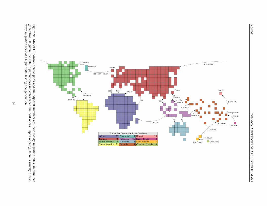
The world of Model C is depicted in Figure 9, with eachcontinent, or independent island, rendered in a differ-ent color. The continents are no longer rectangles butare based on projections of real world geography, witheach country representing approximately 119,000 squaremiles.1 An exception to this is Oceania, where the coun-tries are intended to resemble the major island groups andare typically much smaller in terms of both area and pop-ulation. Clearly, not all of the “continents” in this modelare actual continents, but the name is retained for continu-ity. The distances shown between continents in Figure 9are arbitrary, the only important factor being the numberand migration rate of the ports connecting them.

1The area of sparsely-inhabited northern Siberia has been reduced inthe model.

4.1.1 Migration

The Model C simulations begin in the year 20000 BC, butthe populated areas at that time only include Africa, Eura-sia, Indonesia (including New Guinea), and Australia.Some of the inter-continental ports are already open at thestart of the model and remain at a fixed migration rate.The ports are shown as arrows in Figure 9, labeled withtheir migration rates, in sims per generation. BetweenAfrica and Eurasia, there are ports between modern-dayMorocco and Spain (100 sims/generation), Tunisia andItaly (100 s/g), Egypt and Israel (500 s/g), and betweenEthiopia and Yemen (50 s/g), providing several points ofcontact. Other static ports include a pair between Thai-land and Malaysia (100 s/g), and from the tip of Indonesia(Timor) to Arnhem Land and from New Guinea to CapeYork, both with a rate of just 5 s/g.

The migration rates used in this model are not based onfirm historical data, because such information is, for themost part, unknown (Jorde, 1980). They are based almostentirely on estimates, loosely taking into account prox-imity, population density, and available seafaring tech-nology. Without a firm basis in fact, an attempt wasmade to err on the side of conservatism. Some of themigration rates may be considerably smaller than theyshould be, and many migration routes are undoubtedlymissing. Some readers will disagree with particular de-tails of the timing, location, and migration rate of theseroutes. Greater accuracy will certainly improve the qual-ity of the results generated by the model and our confi-dence in them. However, experience suggests that its re-sults are quite stable and insensitive to all but the mostsignificant changes.

In the previous models, immigrants using a port couldsettle in any random town in the destination country. Asa result, immigrants were immediately assimilated intothe host community. It is more often the case in mod-ern times, and presumably throughout history, that im-migrants will gravitate towards a sub-community of fel-low immigrants who share the same cultural or linguis-tic background. The result is a delay in the exchange oflineages between the immigrants and hosts. This is sim-ulated in the model by having new immigrants initiallychoose from one of five towns, out of up to 46, in the des-tination country. This set of towns is dependent on thesource country from which the migrant came. As a result,immigrants will tend to cluster, though they will not beentirely segregated.

Aside from those already mentioned, the remainder ofthe ports in the model only open at particular points intime, indicated in Figure 9 by the dates in parentheses.Unlike the previous models, in which the entire world wasinhabited from the start, we must now deal with the prob-lem of the initial colonization of new territory. The main

13

RO

HD

EC

OM

MO

NA

NC

ES

TO

RS

OF

AL

LL

IVIN

GH

UM

AN

S

25462821

52648 4

112

23AfricaEurasiaNorth AmericaSouth America

GreenlandIndonesia

OceaniaAustralia

Chatham IslandsNew Zealand

HawaiiEaster Island

Towns Per Country in Each Continent

100 100 500

50 100

Taiwan

Greenland

Hawaii

5 5

New Zealand

10

50

10

10

1

(11000 BC)

(11000 BC)

(2500 BC)

100 (1000−1400 AD)

Iceland

(12000 BC)

10(3000 BC)

10(1600 BC)

10 (1600 BC)

10(1600 BC)

1

(1000 AD)1

(1400 AD)

(400 AD)1

(500 AD)

Society Is.Easter Is.

Chatham Is.

Marquesas Is.

1(300 AD)

Figure9:

Model

C.

Arrow

sdenote

portsand

theadjacent

numbers

aretheir

steadym

igrationrates,

insim

sper

generation.If

given,thedate

inparentheses

indicatesw

henthe

portopens.U

ponopening,there

isusually

afirst-

wave

migration

burstatahigherrate,lasting

onegeneration.

14

ROHDE COMMON ANCESTORS OF ALL LIVING HUMANS

issue this raises is how pioneers are to gain a foothold. Abasic assumption of the model is that sims act indepen-dently in their migration decisions. They cannot organizea sustainable colony in advance, and, because the rate ofmigration to new countries is typically very low, individ-ual migrants will often find themselves isolated and un-able to reproduce. Therefore, the pioneers would tend todie off and it could take quite some time for them to gaina foothold. The result is that earliest migrants into theAmericas and Oceania would not spread out evenly butwould tend to cluster around the port countries, only ad-vancing once the population there reached sufficient den-sity.

Therefore, in order to avoid this problem, any sim whoreaches an uninhabited town is essentially cloned and fivemore sims, of random sex, are created to join him or her.These new sims are given the same parents so the rate oflineage spread is minimally affected. This may be a rea-sonable assumption, given that most organized colonieswere probably quite closely related. With any luck, thisnew colony will be a sustainable, albeit incestuous, breed-ing population. Additionally, newly colonized countrieswill usually have considerably higher than average popu-lation growth rates, as discussed in Section 4.1.2

The port between the eastern tip of Siberia (Chukotka)and Alaska opens in the year 12000 BC. There contin-ues to be scientific debate over the date of the first humanarrival in North America, but this seems to fall at aboutthe median of suggested dates. As with most other newports, this one begins at a higher rate to create an ini-tial wave of migrants. In the first generation, there areabout 100 migrants from Chukotka to Alaska, with 10 inthe reverse direction. Subsequently, the port rate remainsat 10 s/g in both directions. A continuous, low rate ofcontact between Siberia and Alaska following the closeof the Bering land bridge is supported by the availablearchaeological evidence. “It would appear. . . that BeringStrait was never a hindrance to the passage of materialsand ideas among local populations living along both itsshores,” (Arutiunov & Fitzhugh, 1988, pg. 129). It seemsreasonable to assume that this exchange of technology andculture was accompanied by, and perhaps driven by, anexchange of people between the two continents.

One thousand years after the first migrants enter NorthAmerica, ports open between Panama and Columbia (50s/g) and between the Caribbean islands and Venezuela (10s/g). These do not have an initial migration burst, as it isassumed that the earliest inhabitants would have graduallydiffused throughout North America and into South Amer-ica. Much later, in 2500 BC, an additional port opens be-tween Baffin Island and Greenland, to simulate the ad-vance of Pre-Dorset or Independence I Inuit, whose earli-est northern Greenland sites have been dated to 2400 BC(Arutiunov & Fitzhugh, 1988; Grønnow & Pind, 1996).

The Polynesian colonization of the Pacific islands is be-lieved to have had its source in the expansion of the Ta-p’en-k’eng culture from Taiwan into the Philippines andlater into Indonesia. This was followed, around 1600 BC,by the fairly rapid spread of the Lapita culture to Microne-sia and Melasia and then eastward throughout Polyne-sia (Diamond, 1997; Cavalli-Sforza, Menozzi, & Piazza,1994). This is simulated in the model by the opening ofa direct port between Taiwan and the Philippines in 3000BC, with an initial burst of 1000 migrants, settling to anexchange of 10 s/g. In 1600 BC, three more ports open,from the Philippines to the Mariana islands and Microne-sia, and from New Guinea to the Solomons.2

Most of the other inhabitable Pacific islands are thencolonized via the standard inter-country migration mecha-nism. At this early stage, assuming a ChangeCountryProbof 0.05%, the most populous of the islands produce about3 emigrants per generation, most of whom settle in neigh-boring islands. At this rate, it takes about 600 years forthe majority of the island groups to be reached. Note thatthe inter-country migration mechanism does not just sup-port the initial population spread but also the continuousexchange of people between neighboring islands. This isconsistent with the recent view that early Polynesian so-cieties were not entirely isolated (Terrell et al., 1997), andyet the rate of long-distance migration is so low that itwould not seem to contradict the views of critics who ar-gue that such contacts were probably very rare.

Some of the more remote islands are not colonized un-til much later, including Easter Island (Rapa Nui), Hawaii,New Zealand, and the Chatham Islands, which are treatedin the model as separate continents. Easter Island isreached from the Marquesas Islands in 300 AD, with aninitial wave of 50 migrants followed by a steady exchangeof just 1 per generation. Hawaii is reached from the Mar-quesas in 500 AD, with an initial wave of 200 migrants,although there is some question as to whether the firstcolonizers might have come from Tahiti or the Cook Is-lands. Meanwhile, in 400 AD, migrants begin travelingfrom Borneo to Madagascar, with an initial wave of 100.Although there is some question about the source and dateof the first inhabitation of New Zealand, it is settled in themodel from the Society Islands in 1000 AD with an initialwave of 200 migrants. The last place to be populated isthe Chatham Islands, reached from New Zealand in 1400AD by a wave of 100 migrants.

Southern Greenland is known to have been colonizedby Vikings from Iceland in 985 AD. They were visited

2The model is somewhat inaccurate in that the smaller islands of“Near Oceania”, west of and including the Solomons, are not colonizeduntil 1600 B.C., although they are believed to have been inhabited byPleistocene-era people for several thousand years prior to that (Terrell,Hunt, & Gosden, 1997). It is unlikely that this has an effect on the re-sults because there is believed to have been significant contact betweenthe Polynesians and these earlier inhabitants.

15

ROHDE COMMON ANCESTORS OF ALL LIVING HUMANS

regularly for several hundred years and are thought tohave died out or been assimilated by the Inuit sometimebefore 1500. In the model, a port opens from Iceland toGreenland in the year 1000, with 1000 initial inhabitantsfollowed by 100 more per generation until 1400. There isno migration in the reverse direction because of the likeli-hood that no Inuit reached Iceland or other parts of Europeduring the time period in question.

After 1500 AD, several additional large ports, notshown in Figure 9, are opened to simulate colonizationof the Americas and elsewhere. These include migra-tion routes between Spain and Peru, Mexico, and theCaribbean, and between Portugal and Brazil. In 1600,ports open from England to the eastern U.S., from Franceto eastern Canada, from Spain, France and west Africa tothe southern U.S., and from west Africa to the Caribbeanand Brazil. In 1700, a port opens from Denmark to Green-land and in 1800 many more ports open, including vari-ous ones from Europe and China to the U.S., from Eng-land to South Africa, Australia, India, and New Zealand,and from the western U.S., China, and Japan to Hawaii.Most of these ports are quite substantial, with rates be-tween 1,000 and 5,000 immigrants per generation in theprimary direction of colonization, with 100 to 200 in theopposite direction. As discussed in Section 4.1.2, the firstEuropean migrations to North and South America are co-incident with a significant decline in the size of the nativepopulations due to disease.

In order to model generally increased mobility, theNonLocalPortProb was gradually increased towards theend of the simulation. A higher NonLocalPortProb per-mits more sims from outside of the source country to usea port, increasing the overall frequency of long-distancemigration. The initial value of this parameter ranges from2% to 20% in the models tested. In most of the simula-tions, it starts at 5%, but increases to 20% in the year 1500AD, 50% in 1600, 75% in 1700, 85% in 1800, and 90%in 1900. Smaller increases are used for the more con-servative models. The ChangeTownProb also increasesin recent centuries from an initial value of 5% to 10% in1700 and 20% in 1900, with greater increases for the sim-ulations with a baseline of 10%. The ChangeCountryProbalso increases to simulate greater mobility, doubling in theyears 1500, 1750, and 1900.

In addition to the more complex geography and inter-continental ports, a few other details were changed in pro-ducing Model C. The method of selecting fathers in thefirst two models may not have sufficiently taken into ac-count the preference of women to marry single men. As aresult, the process was overly unfair, resulting in too manymen with no children or many children and not enoughwith a few children. This, and some computational con-siderations, led to a new method of choosing fathers thatresults in a slightly more fair distribution of children per

man, as shown in the purple bars in Figure 2. As a re-sult, the percentage of women who will become extinctdecreases to 32.45% and the percentage of extinct mendecreases to 42.92%.

The process of inter-country migration in the first twomodels was more seriously flawed. They used a two-tiered system, with one rate of migration to neighboringcountries and a second rate to all other countries, withthe difference governed by the NonLocalCountryProb pa-rameter. As a result, it was just as likely for someone tomigrate two countries away as it was for them to migrateclear across the continent. Instead, the new model usesa distance-based approach. The overall probability that asim will leave his or her home country is still determinedby the ChangeCountryProb. However, the probability ofreaching any other country in the continent is now propor-tional to the inverse square of the Euclidean distance to thenew country. Thus, the probability of traveling a distanceof 2 countries is 1/4 that of traveling to a neighboringcountry, and the probability of traveling from a countryat the northern tip of South America to one at the south-ern tip is less than 1% that of traveling to a neighboringcountry.

It is important to keep in mind that migration betweencountries is still extremely rare in the model. In the year1500 AD, there will be about 191,000 people in eachcountry in Eurasia, which translates to 111,000 born ev-ery generation. If the ChangeCountryProb is set to 0.05%,which is in the middle of the range to be tested, we can ex-pect only 55.3 sims to leave each country per generation,or 1.8 each year. Because most of these migrants will goto neighboring countries, truly long-distance migrationsonly occur a few times per century. In other continentsand during earlier time periods, population density, andtherefore the number of inter-country migrants, is evenlower. In the same year, Africa and Oceania have about30.0 migrants per generation leaving each country, whileSouth America has 22.1, North America has 17.6, andAustralia has only 0.98. Thus, even the most liberal modelto be tested, which has five times this rate of inter-countrymigration, is still quite conservative in this respect.

4.1.2 Population

Human population density differs throughout the world.Historically, this can be attributed to such factors as cli-mate, disease, and the methods and success of food pro-duction. These differing densities are likely to have asignificant impact on the distribution of common ances-try. Lineage will tend to spread faster, as a function ofdistance, with higher density populations because of thegreater number of migrants.3 It is important, therefore,

3Higher density, more advanced, societies may also have a largerproportion of their citizens migrants, although that is not assumed in the

16

ROHDE COMMON ANCESTORS OF ALL LIVING HUMANS

that the model take into account differing population den-sity throughout the world.

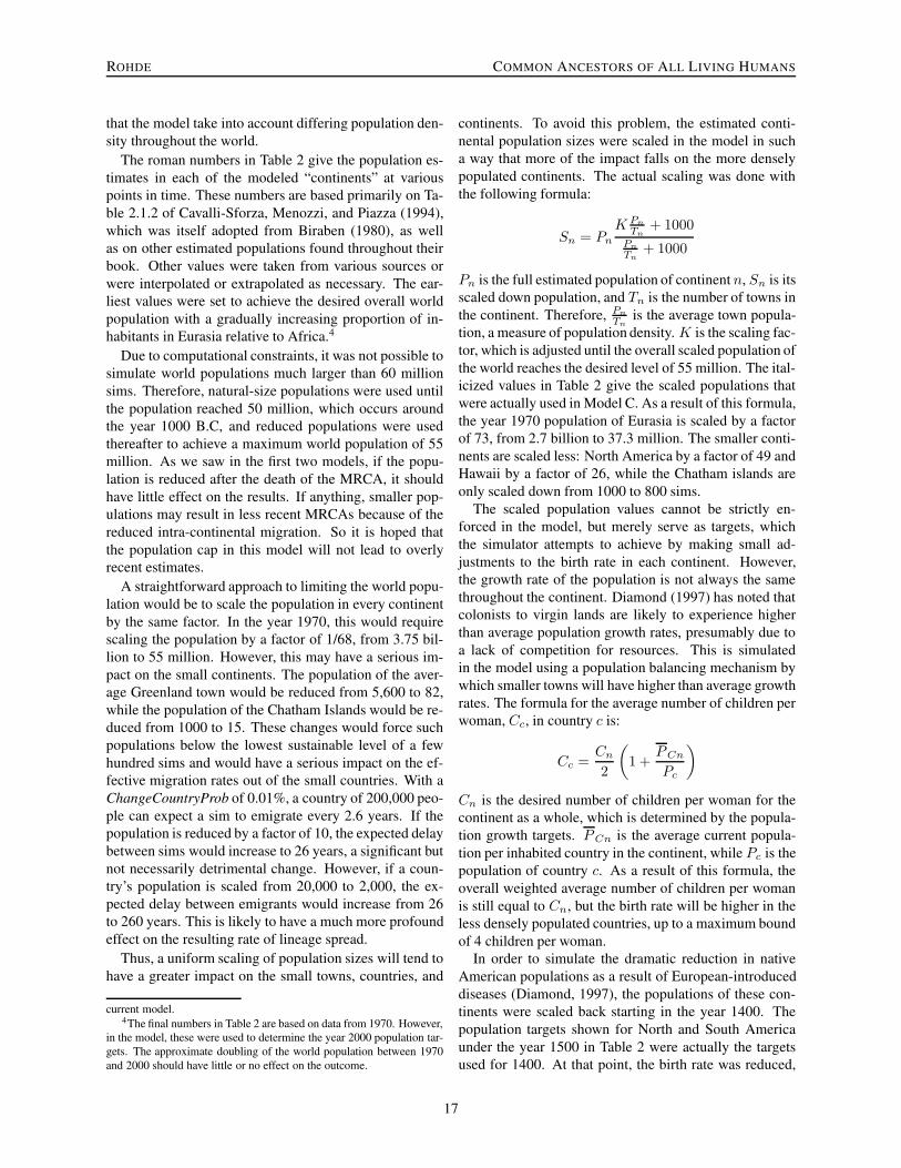
The roman numbers in Table 2 give the population es-timates in each of the modeled “continents” at variouspoints in time. These numbers are based primarily on Ta-ble 2.1.2 of Cavalli-Sforza, Menozzi, and Piazza (1994),which was itself adopted from Biraben (1980), as wellas on other estimated populations found throughout theirbook. Other values were taken from various sources orwere interpolated or extrapolated as necessary. The ear-liest values were set to achieve the desired overall worldpopulation with a gradually increasing proportion of in-habitants in Eurasia relative to Africa.4

Due to computational constraints, it was not possible tosimulate world populations much larger than 60 millionsims. Therefore, natural-size populations were used untilthe population reached 50 million, which occurs aroundthe year 1000 B.C, and reduced populations were usedthereafter to achieve a maximum world population of 55million. As we saw in the first two models, if the popu-lation is reduced after the death of the MRCA, it shouldhave little effect on the results. If anything, smaller pop-ulations may result in less recent MRCAs because of thereduced intra-continental migration. So it is hoped thatthe population cap in this model will not lead to overlyrecent estimates.

A straightforward approach to limiting the world popu-lation would be to scale the population in every continentby the same factor. In the year 1970, this would requirescaling the population by a factor of 1/68, from 3.75 bil-lion to 55 million. However, this may have a serious im-pact on the small continents. The population of the aver-age Greenland town would be reduced from 5,600 to 82,while the population of the Chatham Islands would be re-duced from 1000 to 15. These changes would force suchpopulations below the lowest sustainable level of a fewhundred sims and would have a serious impact on the ef-fective migration rates out of the small countries. With aChangeCountryProb of 0.01%, a country of 200,000 peo-ple can expect a sim to emigrate every 2.6 years. If thepopulation is reduced by a factor of 10, the expected delaybetween sims would increase to 26 years, a significant butnot necessarily detrimental change. However, if a coun-try’s population is scaled from 20,000 to 2,000, the ex-pected delay between emigrants would increase from 26to 260 years. This is likely to have a much more profoundeffect on the resulting rate of lineage spread.

Thus, a uniform scaling of population sizes will tend tohave a greater impact on the small towns, countries, and

current model.4The final numbers in Table 2 are based on data from 1970. However,

in the model, these were used to determine the year 2000 population tar-gets. The approximate doubling of the world population between 1970and 2000 should have little or no effect on the outcome.

continents. To avoid this problem, the estimated conti-nental population sizes were scaled in the model in sucha way that more of the impact falls on the more denselypopulated continents. The actual scaling was done withthe following formula:

Sn = Pn

K Pn

Tn+ 1000

Pn

Tn+ 1000

Pn is the full estimated population of continent n, Sn is itsscaled down population, and Tn is the number of towns inthe continent. Therefore, Pn

Tnis the average town popula-

tion, a measure of population density. K is the scaling fac-tor, which is adjusted until the overall scaled population ofthe world reaches the desired level of 55 million. The ital-icized values in Table 2 give the scaled populations thatwere actually used in Model C. As a result of this formula,the year 1970 population of Eurasia is scaled by a factorof 73, from 2.7 billion to 37.3 million. The smaller conti-nents are scaled less: North America by a factor of 49 andHawaii by a factor of 26, while the Chatham islands areonly scaled down from 1000 to 800 sims.

The scaled population values cannot be strictly en-forced in the model, but merely serve as targets, whichthe simulator attempts to achieve by making small ad-justments to the birth rate in each continent. However,the growth rate of the population is not always the samethroughout the continent. Diamond (1997) has noted thatcolonists to virgin lands are likely to experience higherthan average population growth rates, presumably due toa lack of competition for resources. This is simulatedin the model using a population balancing mechanism bywhich smaller towns will have higher than average growthrates. The formula for the average number of children perwoman, Cc, in country c is:

Cc =Cn

2

(

1 +P Cn

Pc

)

Cn is the desired number of children per woman for thecontinent as a whole, which is determined by the popula-tion growth targets. P Cn is the average current popula-tion per inhabited country in the continent, while Pc is thepopulation of country c. As a result of this formula, theoverall weighted average number of children per womanis still equal to Cn, but the birth rate will be higher in theless densely populated countries, up to a maximum boundof 4 children per woman.

In order to simulate the dramatic reduction in nativeAmerican populations as a result of European-introduceddiseases (Diamond, 1997), the populations of these con-tinents were scaled back starting in the year 1400. Thepopulation targets shown for North and South Americaunder the year 1500 in Table 2 were actually the targetsused for 1400. At that point, the birth rate was reduced,

17

ROHDE COMMON ANCESTORS OF ALL LIVING HUMANS

Table 2: Continental populations, in thousands, at various points in time. Roman numbers are estimates of the truepopulations. The italic numbers below them are the rescaled values used in the Model C simulations to achieve amaximum world population of 55 million.

Continent 20K BC 15K BC 10K BC 5K BC 2K BC 1K BC 500 BC 1 AD 500 AD 1000 1250 1500 1750 1970Eurasia 1230 2030 2850 3350 18700 38800 125000 217000 158000 193000 323000 320000 629000 2722000

1230 2030 2850 3350 18700 38800 43979 44288 40251 38814 38513 34170 41655 37307Africa 670 870 950 1100 3220 5290 17000 26000 31000 39000 58000 87000 104000 353000

670 870 950 1100 3220 5290 6735 6371 8474 8434 7737 9474 7880 6192S. America 0 0 50 200 1500 3000 4000 5000 8000 12000 23000 40000 15000 283000

0 0 50.0 200 1500 3000 1882 1679 2556 2925 3271 4435 1876 4234N. America 0 0 50 200 1000 1500 2000 3000 5000 10000 20000 35000 5000 228000

0 0 50.0 200 1000 1500 1348 1581 2293 3195 3755 4862 1733 4639Indonesia 50 50 50 100 500 1000 1000 2000 3000 5000 8000 12000 16000 119000

50.0 50.0 50.0 100 500 1000 545 689 995 1227 1215 1462 1340 1788Australia 50 50 50 50 70 100 100 100 100 100 200 250 250 20000

50.0 50.0 50.0 50.0 70.0 100 66.1 59.5 61.6 59.2 81.2 88.2 83.0 317Oceania 0 0 0 0 0 300 1000 1000 1000 1000 2000 3000 3000 19000

0 0 0 0 0 300 439 329 364 324 381 449 366 430New Zeal. 0 0 0 0 0 0 0 0 0 2 50 100 150 3000

0 0 0 0 0 0 0 0 0 1.9 18.6 24.9 26.3 53.8Hawaii 0 0 0 0 0 0 0 0 0 20 50 100 200 800

0 0 0 0 0 0 0 0 0 12.3 19.1 25.5 30.3 30.7Greenland 0 0 0 0 10 10 10 10 10 15 15 20 25 56

0 0 0 0 10.0 10.0 6.5 5.9 6.1 7.5 6.9 7.8 8.1 9.0Chatham Is. 0 0 0 0 0 0 0 0 0 0 0 2 2 1

0 0 0 0 0 0 0 0 0 0 0 1.4 1.4 0.8Easter Is. 0 0 0 0 0 0 0 0 2 5 10 10 2 0

0 0 0 0 0 0 0 0 1.2 2.0 2.5 2.4 1.1 0Total 2000 3000 4000 5000 25000 50000 150110 254110 206112 260142 434325 497482 772629 3747860

2000 3000 4000 5000 25000 50000 55000 55002 55001 55001 55000 55002 55000 55001

causing the loss of much of the native population. Therate of this decline reached its peak around the year 1500,as Europeans began to arrive. The net effect of this wassomewhat greater than intended, resulting in the loss of97% of North Americans and 93% of South Americansbefore the populations began to recover in 1570. Diamondestimates that the actual decline may have been as large as95%. It is unlikely that the more severe decline in NorthAmerica will have a noticeable effect on the results of thesimulation.

Because the population density varies between conti-nents, the number of towns per country was adjusted toproduce towns of reasonable average size. These countsare given in Figure 9. In the year 1500 AD, the primar-ily agricultural continents have approximately 4,000 in-habitants per town. The primarily non-agricultural con-tinents, including North America, Australia, Greenland,and Easter Island had approximately 2,000 inhabitants pertown, while the Chatham Islands had 500. Overall, ModelC contains 497 countries and 15,059 towns.

4.2 ResultsAgain, it should be stressed that we do not have sufficientdata to fix the parameters of the model with much cer-tainty. Therefore, a series of simulations was conducted

to determine a range of possible outcomes. The resultsare shown in Figure 10. For each set of parameters, atleast six trials were performed and their resulting datesaveraged. The results tend to be somewhat less consistentacross trials in this model than in the previous ones, withMRCA and ACA dates having a coefficient of variation ofbetween 6% and 10%.

The first three simulations were intended to test liberal,moderate, and conservative parameter sets. In the “lib-eral” simulation, C1, the ChangeTownProb was 20%, theChangeCountryProb was 0.25%, the NonLocalPortProbwas 20%, and the port rates were actually 10 times thevalues shown in Figure 9. The resulting MRCA date was1945 BP and the ACA date was 4158 BP, which do in-deed seem remarkably recent. The case could be madethat simulation C1 is not excessively liberal. The Change-TownProb of 20% is in line with the finding of Adams andKasakoff (1976) that a natural threshold exists across soci-eties for groups with an 80% endogamy rate. The Change-CountryProb of 0.25% means that the average countrythroughout the final 2500 years of the simulation has just5.3 emigrants per year, with many having much fewer.Prior to 500 B.C., emigration rates were even lower be-cause of the smaller populations. Furthermore, even withport rates that are ten times those shown in Figure 9, most

18

ROHDE COMMON ANCESTORS OF ALL LIVING HUMANS

Sim

ulat

ion

Cha

ngeT

ownP

rob

Cha

ngeC

ount

ryPr

obPo

rtRat

eSca

leN

onLo

calP

ortP

rob

Comment Common Ancestry Timeline

16K 14K 12K 10K 8K 6K 4K 2K 0Years Before Present

No Common Ancestors

Some Common Ancestors

All Common Ancestors

C1) 20% 0.25% 10 20% Liberal

C2) 5% 0.05% 1 5% Moderate

C3) 2% 0.01% 0.1 2% Conservative

C4) 5% 0.05% 1 5% Max Population 25M

C5) 20% 0.05% 1 5% Higher ChangeTownPr

C6) 2% 0.05% 1 5% Lower ChangeTownPr

C7) 5% 0.25% 1 5% Higher ChCountryProb

C8) 5% 0.01% 1 5% Lower ChCountryProb

C9) 5% 0.05% 10 5% Higher PortRate

C10) 5% 0.05% 0.1 5% Lower PortRate

C11) 5% 0.05% 1 20% Higher NonLocalPortPr

C12) 5% 0.05% 1 2% Lower NonLocalPortPr

C13) 5% 0.05% 1 0% All Local Port Users

C14) 5% 0.05% 1 5% Geometric Distance Fn

C15) 5% 0.05% 1 5% No Post-1500 Changes

C16) 5% 0.05% 1 5% Other Routes to Amer.

Figure 10: Results of the Model C simulations.

19

ROHDE COMMON ANCESTORS OF ALL LIVING HUMANS

of the land bridges, with the exception of Sinai, still haveonly about 33 migrants per year, while the long-term nau-tical bridges average 3.3 or fewer migrants per year.

Nevertheless, it is possible that some of the parametersused in simulation C1 permit too much mobility. There-fore, C2 was conducted with more conservative parame-ters. The ChangeTownProb and NonLocalPortProb wereboth reduced to 5%, the ChangeCountryProb was reducedby a factor of 5 and the port rates by a factor of ten. Thesechanges increase both the MRCA and ACA dates by about75%, resulting in an MRCA date of 3415 BP and an ACAdate of 7353. But the primary finding remains that ourmost recent common ancestor most likely lived within thepast few thousand years, much more recently than Mito-chondrial Eve or Y-Chromosome Adam.

The blue curve in Figure 4 shows the percentage ofcommon ancestors as a function of time for one of theC2 trials. After an initially slow climb, the percentage ofCAs increases quite rapidly and smoothly until it beginsto slow at around 75%. This is the point at which mostof the countries in Eurasia, Indonesia, and Africa containCAs and the growth in the percentage of CAs slows asthese continents saturate. This occurs at around the 90%mark, at which point the curve noticeably levels. The re-mainder of the growth involves the slower spread of com-mon ancestry throughout North and South America andAustralia. On average, the C2 sims reach 95% CAs in theyear 5920 BP, 98% in 6399 BP, and 99% in 6584 BP, butdo not reach 100% CAs until 7353 BP. Thus the point atwhich nearly everyone is a CA and the point at which trulyeveryone is a CA are separated by perhaps 1000 years.

In the interest of more firmly bounding the range ofpossible CA dates, a third simulation was conducted thatis even more conservative than C2. C3 uses a Change-TownProb of 2%, a ChangeCountryProb of 0.01%, a Non-LocalPortProb of 2% and port rates that are 1/10 thoseshown in Figure 9. The resulting MRCA appears in 7110BP and the ACA point moves back to 15042 BP. In thiscase there is a proportionately longer tail on the transi-tion from the MRCA to the ACA point, with 99% CAs by13087 BP. The role of the individual parameters in pro-ducing these less recent dates, and the reasonableness ofthose settings, are discussed in the next section.

4.2.1 Parameter effects

Simulations C4–C16 are variations on C2, exploring theeffects of individual parameter changes to better under-stand the model. To aid the comparison, vertical linesin Figure 10 mark the approximate C2 MRCA and ACApoints. The first question investigated is the possible ef-fect of the population cap of 55 million. Although run-ning simulations with larger populations was not possibleon the available computers, simulation C4 was conducted

with a population cap of 25 million, reached in 2000 BC.The result is absolutely no change in the MRCA date,while the ACA date was 2.4% more recent, a differencethat does not approach significance. Therefore, it is likelythat further growth beyond 55 million would not substan-tially change the model’s predictions. As we saw in Mod-els A and B, larger populations can actually result in morerecent dates with conservative migration, but have littleeffect with more liberal migration.

Simulations C5 and C6 vary the ChangeTownProb, orthe percent of sims who leave their home town. Increas-ing this value from 5% to 20% causes a 8.3% reductionin the MRCA time and a 10.4% reduction in the ACAtime. Decreasing it to 2%, which is perhaps the minimalreasonable level given our definition of a town, causesno change in MRCA, although the ACA time increasesby 7.9%. Because there is reasonably frequent migrationwithin a country even at the lowest reasonable Change-TownProb setting, this parameter has relatively little effecton the model.

In contrast, the model is more sensitive to variations inthe ChangeCountryProb within the rather wide range ofplausible values. Increasing this parameter by a factor of5 to 0.25% in simulation C7 causes a 23.7% reduction inMRCA and a 26.2% reduction in ACA. Conversely, de-creasing this parameter by a factor of 5 pushes the MRCAto 5103 BP in simulation C8, with an ACA point of 12648BP. With a ChangeCountryProb of 0.01%, the averagecountry in the year 1500 has only one emigrant every 4.7years, most of which will head to neighboring countriesand some of which may not even produce children. Lesspopulated countries will have even fewer emigrants andthere will also be many fewer early in the simulation be-cause of the lower population densities. In the year 5,000BC, the average inhabited country will have just one em-igrant every 48 years. A ChangeCountryProb any lowerthan this may be unreasonably conservative.

Another important factor is the migration rate acrossinter-continental ports. The default rates shown in Fig-ure 9, which were used in Simulation C2, were intendedto be quite low. Scaling these rates up by a factor of 10, inC9, results in an 18.2% decrease in the MRCA time anda 21.1% decrease in the ACA time. Scaling down by afactor of 10, C10, produces a 10.1% increase in MRCAtime and a 17.5% increase in ACA time. Therefore, themodel is fairly sensitive to the port rates, but not nearly somuch as it is to the ChangeCountryProb, which governsthe majority of the migration throughout the world.

The percentage of port users who do not originate inthe port’s source country, the NonLocalPortProb, was ma-nipulated in simulations C11–C13. Increasing this valueto 20% or reducing it to 0% has very little effect on theMRCA time and a somewhat larger effect on the ACAtime. Thus, the existence of migrants who travel long dis-

20

ROHDE COMMON ANCESTORS OF ALL LIVING HUMANS

tances to use a port is not integral to the outcome of themodel.

One reasonable concern, however, is that the model per-mits too much long distance migration within continents.In most of the Model C simulations, the probability ofemigration to another country is proportional to the in-verse square of the distance between the countries. As aresult, really long distance journeys across continents arerare, but not exceedingly so. A stricter assumption mightbe that migration falls off geometrically with distance. Insimulation C14, the probability of migration between twocountries separated by distance d is proportional to 2−d.As a result, very long distance migration is much lesscommon. This increases the MRCA time by 7.2% andthe ACA time by 16.0%.

4.2.2 Other experiments

Much has changed in the world in the last 500 years. Ofparticular interest to us is the continuing increase in geo-graphic and social mobility in general and the large move-ments of people to particular areas including the Europeancolonization of the Americas, Australia, New Zealand,and parts of Africa. Ultimately, these changes will re-sult in a much more recent common ancestor, eventuallyapproaching the predictions of Chang’s panmictic model.One question, however, is what effects these relatively re-cent changes may have had so far on the common ances-tors of people living today.

As described in Section 4.1.1, the model C simulationsreported thus far involved numerous post-1500 changes,such as the opening of 16 large ports to the Americas andother areas and overall increases in the migration rates.But these additions were far from comprehensive. So wemight ask whether the current additions have had any sub-stantial effect on the results and, therefore, whether moreadditions could be expected to further alter the outcome.

Simulation C15 was designed to test the effect of thecurrent post-Columbian changes by eliminating them en-tirely. This simulation was identical to C2 until 1400, afterwhich the population sizes remained stable and no addi-tional ports were created or parameters were altered. Thishad virtually no effect, actually decreasing the MRCAtime by 2.3% and the ACA time by 1.3%, both highlynon-significant. This suggests that the changes in humanmigration patterns over the past 500 years may still be toorecent to have had much of an effect on our common an-cestry, though they will certainly do so in the centuries tocome.

There has been considerable debate over the likelihoodthat the Americas were reached, prior to Columbus, viaroutes other than the Bering Strait. These include possiblecontact between Vikings and native Americans in New-foundland, in addition to those that may have occurred

in Greenland, and, more significantly, contact betweenSouth America and the Pacific Islands. The primary evi-dence for the latter appears to be the spread of the sweetpotato, believed to be of South American origin, through-out much of Oceania around 1500 years ago (Bellwood,1979). If such alternate routes to the New World existed,how might they have affected our common ancestry?

This question was addressed with a variant of simula-tion C2. In C16, two ports were created in 400 AD, be-tween Peru and the Marquesas Islands and between Chileand Easter Island, with migration rates of 10 s/g in eachdirection. In addition, a one-directional port was createdfrom southern Greenland to Newfoundland lasting from1000 to 1350 AD, also with a rate of 10 s/g. As shownin Table 10, this resulted in a statistically significant 8.8%decrease in MRCA time and a 4.6% decrease in ACA time(n.s.). Therefore, the possible existence of continued con-tacts with the Americas other than through Beringia mayhave had some effect on the dates of our common ances-tors, but such contacts are not critical to the existence of arecent common ancestor.

5 Further analysesTo this point, most of the discussion in this paper has fo-cused on the dating of our MRCA and the point at whichall ancestors were shared in common. But, assuming themodel is sufficiently accurate in its design and details,many other interesting predictions about our common an-cestors and ourselves can be drawn from it.

5.1 Who was our most recent commonancestor?

So who was our most recent common ancestor? Was it aman or a woman? Where did he or she live? One mightpredict that the MRCA is likely to be someone, perhaps anancient king, with many children who quickly migratedfar from home. It turns out that the reality may be far lessglamorous.

Studying the MRCAs of several Model C simulations,reveals that the most recent CAs lived either in southeastor northeast Asia, nearly always in a port country. Themost common sites are Taiwan and Malaysia in the south-east and in the Chukotka and Kamchatka regions of north-east Russia, close to the Bering Strait. Living near a portis an obvious advantage because it allows one’s descen-dants to rapidly reach a second continent. The reason thatthe MRCAs arise in either southeast or northeast Asia andnot, for example, the Middle East, is their proximity toOceania and North America, respectively. Because Ocea-nia was settled quite late and relatively slowly, and be-cause Australia has infrequent contact with the rest of the

21

ROHDE COMMON ANCESTORS OF ALL LIVING HUMANS

world, it is advantageous, from the perspective of tryingto become a CA, to live in this gateway to the Pacific.Likewise, it is also an advantage to live near the gatewayto the Americas because the tip of South America is alsodifficult to reach. As a result, quite recent CAs emergethroughout far eastern Asia, including Japan and coastalChina.

There has been considerable debate in recent years overthe site of modern human origins. The multitude of ho-minid fossils found in east Asia has suggested to someresearchers that modern humans may have evolved there,either solely or in parallel with their evolution in otherparts of the world (Thorne & Wolpoff, 1992; Wu, Poirier,Wu, & Wu, 1995; Etler, 1996). However, the prevailingview, based primarily on the analysis of genetic markers,now seems to be that humans first arose in Africa beforespreading to east Asia and throughout the world (Wilson& Cann, 1992; Jin & Su, 2000; Ke et al., 2001). Even ifthe origin of modern humans is not to be found in eastAsia, perhaps it will be some small consolation to themulti-regionalist to know that the much more recent com-mon ancestors of all humans very likely did live there.

Figure 11 shows the year in which the first CA arisesin each country in one trial of simulation C2. In this trial,the MRCA was a man living in Taiwan, born in 3536 BPand who died in 3459 BP. Other CAs arose in Kamchatkaand southern China within a few decades, working back-wards in time, and then at various other locations in east-ern Asia, both north and south. Within 600 years of theMRCA, CAs can be found throughout most of Eurasia,much of Indonesia, and some of north Africa. It takes an-other 2500 years for the CAs to appear in the more remoteparts of North and South America. Note that no CAs livedin Greenland or Oceania because those areas were not yetinhabited.

By studying the immediate descendants of the MRCAs,we can get a better sense of who they may have been andhow they earned that title. An average sim living at thetime of the MRCAs has about 2.09 adult children. In con-trast, a sampling of 130 first-generation CAs (FGCAs),none of whose descendants were also CAs, from simu-lation C2 had an average of 5.0 children. This is morethan twice the overall average, but it is not an exceptionalnumber. Only 5% of these CAs had more than 10 chil-dren, while 20% had just three children and 12% had only2 children. The advantage for the FGCAs stems from thefact that their families happen to have maintained higherthan average reproductive levels over the course of a fewgenerations. The average number of children per descen-dant in the second generation is 2.63, followed by 2.28 inthe third generation. Subsequently, birth rates are at aver-age levels. As a result, although an average person at thattime has 40 great great great grandchildren, the averageFGCA has 130. Because the FGCAs do not tend to be

the very rare sort of person with many children, there isno special advantage for men in this regard and just abouthalf of the FGCAs were women. This is partially drivenby the fact that husbands and wives tend to become MR-CAs together.

One might expect, however, that an FGCAs descen-dants are likely to have disbursed very rapidly, but thatis not always the case. 73% of the FGCAs had no descen-dants move out of the country in the first four generations,and 51% had no descendants migrate in the first five gen-erations. Of the 22,710 descendants of the 130 FGCAs inthe first five generations, only 34 moved away from theirhome country, a rate that is about three times the Change-CountryProb. But of these, about a third reached a dif-ferent continent. Therefore, the widespread disbursementof the lineages of MRCAs does not usually begin immedi-ately. Their families grow gradually, at a somewhat higherthan average rate, and then disburse gradually, also at asomewhat higher than average rate. The main advantagecomes not in being extraordinarily prolific, but in livingnear the geographic center of the world and near a conti-nental boundary so one’s descendants reach another con-tinent within a relatively short time.

It is interesting to track the descendants of a single oneof these MRCAs throughout the course of a simulationto discover when they first arrived in each part of theworld. The results, mapped in Figure 12, are in appear-ance very similar to those for the first occurrence of anMRCA in each country, but in this case we are workingin the opposite direction in time. This particular MRCAwas born in Taiwan in 1536 BC. She had a remarkable ad-vantage in that one of her great grandchildren migrated upthe coast to Chukotka. Other early descendants migratedthroughout southeast Asia, with some heading to centralRussia. Her lineage first reached Indonesia in 1206 BC,North America in 1091 BC, Africa in 838 BC, Australiain 652 BC, South America in 95 BC, and Greenland in381 AD. Some of the last places reached were southernArgentina in 855 AD, and New Zealand in 1116 AD andthe Chathams in 1419 AD, in the first wave of their colo-nizations.

It appears that our MRCAs were not necessarily re-markable people. They could have been men or womenof any social standing, who, most of the time, just hap-pen to have been living at a crossroads. However, thisfinding may simply be a reflection of the model’s assump-tions. The model does not allow for the fact that an ancientruler may have achieved the status of MRCA by father-ing many sons who, through continued wealth and power,themselves produced many children (Zerjal et al., 2003).Such a dynasty, if it existed in the right time and place,could have reduced the MRCA time. It is also importantto keep in mind that the MRCA of all living humans is nota fixed person and will change over time. With the ever

22

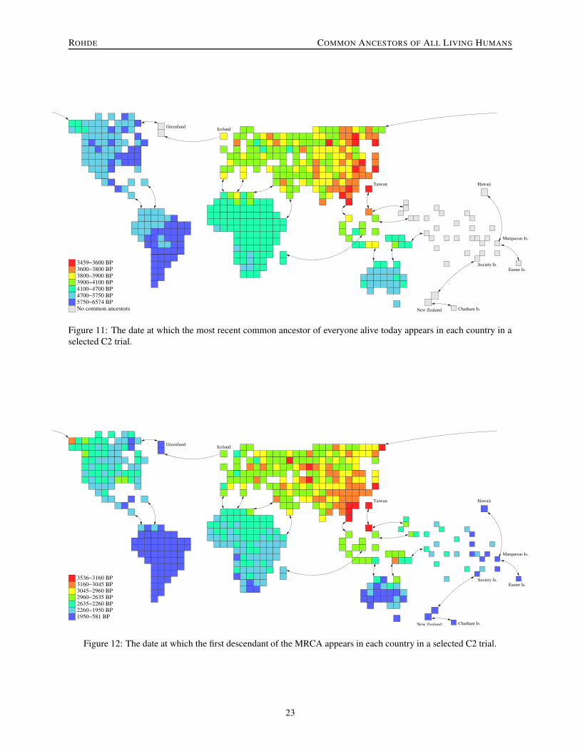
ROHDE COMMON ANCESTORS OF ALL LIVING HUMANS

3800−3900 BP3900−4100 BP4100−4700 BP4700−5750 BP5750−6574 BP

3459−3600 BP3600−3800 BP

No common ancestors

Taiwan

Greenland

Hawaii

New Zealand

Iceland

Society Is.Easter Is.

Chatham Is.

Marquesas Is.

Figure 11: The date at which the most recent common ancestor of everyone alive today appears in each country in aselected C2 trial.

3536−3160 BP

3045−2960 BP

2260−1950 BP1950−581 BP

3160−3045 BP

2960−2635 BP2635−2260 BP

Taiwan

Greenland

Hawaii

New Zealand

Iceland

Society Is.Easter Is.

Chatham Is.

Marquesas Is.

Figure 12: The date at which the first descendant of the MRCA appears in each country in a selected C2 trial.

23

ROHDE COMMON ANCESTORS OF ALL LIVING HUMANS

growing mobility of the world’s people, both geograph-ically and socially, the MRCA will, relatively speaking,become increasingly recent.

5.2 Common ancestors of subpopulationsAlthough we have been looking at the common ances-tors of everyone alive in the world today, one might won-der whether certain sub-populations, such as Europeans,share much more recent common ancestors. Starting witha trial from an earlier version of model C, which had aworld-wide MRCA date of 3520 BP and an ACA date of11380 BP, the ancestry of just the present-day sims livingin Europe, east of the Black Sea, was tracked. The result-ing MRCA appeared in 2120 BP, about 40% more recentthan the worldwide MRCA. Although the worldwide MR-CAs in the model nearly always live in east Asia, the firstfew European MRCAs were spread around Eurasia, withthe first one appearing close to Israel or Jordan, and withothers in Japan in 142 BC, in Siberia in 169 BC, in Burmain 172 BC, and in Iraq in 185 BC. Interestingly, the ACApoint is exactly the same for Europe as it is for the worldas a whole.

Given that the MRCAs for Europe are scatteredthroughout Eurasia, it should not be too surprising thatthe MRCA for all of Eurasia was nearly as recent, dyingjust 40 years earlier, in 2160 BP. The MRCAs for Eura-sia arise first around Thailand and Burma, southern India,and southern China. The MRCA for Eurasia together withAfrica in this simulation lived about 300 years earlier,in 2450 BP. They first arise scattered throughout Eura-sia, first in Korea, then Uzbekistan, Spain, and Siberia.But these are results of a single trial and there is prob-ably nothing significant about these particular locations.The most recent of the CAs who lived in Africa appear inEgypt, as one might expect, in 2530 BP.

5.3 Genetic inheritanceThe point was made earlier that the existence of an ACAdate, or a time at which everyone alive today shares thesame set of ancestors, does not necessarily imply that weowe the same degree of ancestry to each of those peo-ple. Otherwise, it is unlikely that even the most superfi-cial physical differences could have arisen since then. Butthe question is, to what extent does the ancestral inheri-tance of various peoples in the world today differ? Arethe differences subtle or dramatic?

We can begin to answer these questions by tracing theancestry of individual present-day sims. But in this case,we are not just interested in the identity of the ancestors,but in the percentage of the sim’s genes attributable toeach ancestor. We will assume that a sim owes exactly1/2 of his genes to each of his parents, and thus 1/4 to

each grandparent, and so on. Of course, if an ancestorappears more than once on the family tree, she will con-tribute the sum of the individual proportions. After manygenerations, the proportion of genes contributed by eachancestor becomes vanishingly small, until some ancestorsmay contribute no actual genes. But we can sum the pro-portions over each continent or country to get a picture ofthe percentage of genes the modern sim owes to ancestorsliving in various parts of the world at a given time.

We will first trace the ancestry of a randomly selectedJapanese sim born in the year 2000 in one of the C2 tri-als. By 1500 AD, the sim owes 98.8% of his ancestry tohis home country, the middle of the three Japanese terri-tories, and much of the rest to the other two countries thatform Japan. The remaining 0.4% is traceable to neighbor-ing areas of China and Korea. By 500 AD, 98.9% of thesim’s ancestry is still attributable to Japan as a whole. Thisdeclines to 97.5% by 2000 BC, 95.7% by 5000 BC, and88.4% by 20000 BC. The proportion of the sim’s ances-try attributable to each country in the world in 5000 BC isshown in Figure 13. The red and orange regions togetheraccount for 97.35% of the ancestry, with 2.62% from therest of Eurasia, 0.014% from Africa, 0.00090% from In-donesia and Australia, and 0.00086% from the Americas.

Figure 14 shows the corresponding ancestry for a ran-domly selected Norwegian. In this case, 92.3% of the an-cestry in the year 5000 BC is attributable to the country inwhich the sim lives, in central Norway, and 96% to Scan-dinavia as a whole. The Norwegian has about three timesas much African ancestry as the Japanese sim, but muchless American, Indonesian, and Australian. The Norwe-gian owes 0.00044% of his ancestry to 5000 BC Japan,while the Japanese owes 0.00049%, or about 1 part in200,000, to ancient Norway. That would suggest that,at this rate of mixing, a typical Norwegian might be ex-pected to have inherited about one haplotype block from5000 BC Japan (Gabriel et al., 2002).

Therefore, because of the fairly low migration rates ofsimulation C2, the genetic inheritance of this randomlyselected sim derives almost entirely from nearby areas,even looking 7000 years into the past. Given the quiterecent MRCA date of 1460 BC in this trial, it may be sur-prising that the sim’s ancestry remains so highly concen-trated after such a long period. This serves to highlightboth how conservative the parameters of the simulationsactually are and the remarkable fact that a fairly recentMRCA emerges despite these conservative parameters.

The ancestry of a central African is shown in Figure 15.The pattern of tightly clustered ancestry is similar to thatof the previous two examples, but in this case the Africanhad two major ancestral branches, one in his home coun-try and another stemming from a great-grandparent fromthe Ghana area. The African sim has almost entirelyAfrican ancestry, with 0.00092% Eurasian ancestry, pri-

24

ROHDE COMMON ANCESTORS OF ALL LIVING HUMANS

> 1e−11e−1 − 1e−31e−3 − 1e−41e−4 − 1e−71e−7 − 1e−91e−9 − 1e−12< 1e−12No ancestors

Taiwan

Greenland

Hawaii

New Zealand

Iceland

Society Is.Easter Is.

Chatham Is.

Marquesas Is.

Figure 13: The fraction of ancestry of a randomly selected Japanese sim, who was born in 2000, that is traceable toeach country in 5000 BC.

> 1e−11e−1 − 1e−31e−3 − 1e−41e−4 − 1e−71e−7 − 1e−91e−9 − 1e−12< 1e−12No ancestors

Taiwan

Greenland

Hawaii

New Zealand

Iceland

Society Is.Easter Is.

Chatham Is.

Marquesas Is.

Figure 14: The fraction of ancestry of a randomly selected Norwegian sim, who was born in 2000, that is traceable toeach country in 5000 BC.

25

ROHDE COMMON ANCESTORS OF ALL LIVING HUMANS

> 1e−11e−1 − 1e−31e−3 − 1e−41e−4 − 1e−71e−7 − 1e−91e−9 − 1e−12< 1e−12No ancestors

Taiwan

Greenland

Hawaii

New Zealand

Iceland

Society Is.Easter Is.

Chatham Is.

Marquesas Is.

Figure 15: The fraction of ancestry of a randomly selected central African sim, who was born in 2000, that is traceableto each country in 5000 BC.

> 1e−11e−1 − 1e−31e−3 − 1e−41e−4 − 1e−71e−7 − 1e−91e−9 − 1e−12< 1e−12No ancestors

Taiwan

Greenland

Hawaii

New Zealand

Iceland

Society Is.Easter Is.

Chatham Is.

Marquesas Is.

Figure 16: The fraction of ancestry of a randomly selected Mexican sim, who was born in 2000, that is traceable toeach country in 5000 BC.

26

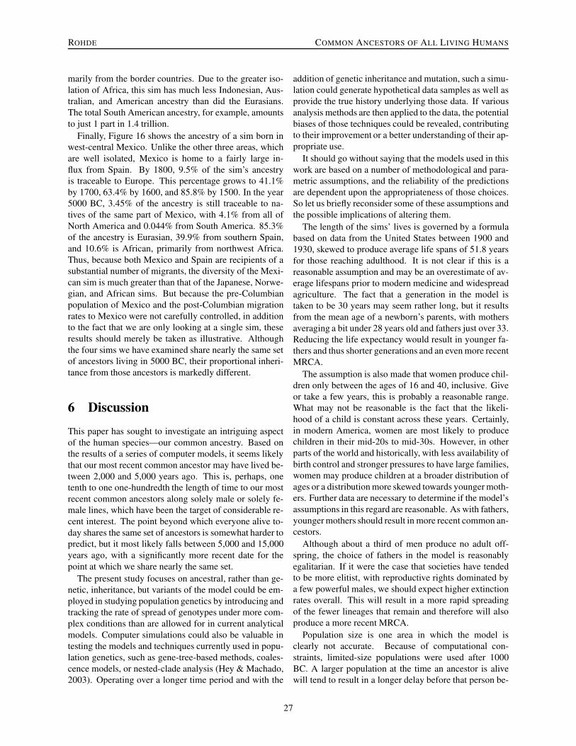
ROHDE COMMON ANCESTORS OF ALL LIVING HUMANS

marily from the border countries. Due to the greater iso-lation of Africa, this sim has much less Indonesian, Aus-tralian, and American ancestry than did the Eurasians.The total South American ancestry, for example, amountsto just 1 part in 1.4 trillion.

Finally, Figure 16 shows the ancestry of a sim born inwest-central Mexico. Unlike the other three areas, whichare well isolated, Mexico is home to a fairly large in-flux from Spain. By 1800, 9.5% of the sim’s ancestryis traceable to Europe. This percentage grows to 41.1%by 1700, 63.4% by 1600, and 85.8% by 1500. In the year5000 BC, 3.45% of the ancestry is still traceable to na-tives of the same part of Mexico, with 4.1% from all ofNorth America and 0.044% from South America. 85.3%of the ancestry is Eurasian, 39.9% from southern Spain,and 10.6% is African, primarily from northwest Africa.Thus, because both Mexico and Spain are recipients of asubstantial number of migrants, the diversity of the Mexi-can sim is much greater than that of the Japanese, Norwe-gian, and African sims. But because the pre-Columbianpopulation of Mexico and the post-Columbian migrationrates to Mexico were not carefully controlled, in additionto the fact that we are only looking at a single sim, theseresults should merely be taken as illustrative. Althoughthe four sims we have examined share nearly the same setof ancestors living in 5000 BC, their proportional inheri-tance from those ancestors is markedly different.

6 Discussion

This paper has sought to investigate an intriguing aspectof the human species—our common ancestry. Based onthe results of a series of computer models, it seems likelythat our most recent common ancestor may have lived be-tween 2,000 and 5,000 years ago. This is, perhaps, onetenth to one one-hundredth the length of time to our mostrecent common ancestors along solely male or solely fe-male lines, which have been the target of considerable re-cent interest. The point beyond which everyone alive to-day shares the same set of ancestors is somewhat harder topredict, but it most likely falls between 5,000 and 15,000years ago, with a significantly more recent date for thepoint at which we share nearly the same set.

The present study focuses on ancestral, rather than ge-netic, inheritance, but variants of the model could be em-ployed in studying population genetics by introducing andtracking the rate of spread of genotypes under more com-plex conditions than are allowed for in current analyticalmodels. Computer simulations could also be valuable intesting the models and techniques currently used in popu-lation genetics, such as gene-tree-based methods, coales-cence models, or nested-clade analysis (Hey & Machado,2003). Operating over a longer time period and with the

addition of genetic inheritance and mutation, such a simu-lation could generate hypothetical data samples as well asprovide the true history underlying those data. If variousanalysis methods are then applied to the data, the potentialbiases of those techniques could be revealed, contributingto their improvement or a better understanding of their ap-propriate use.

It should go without saying that the models used in thiswork are based on a number of methodological and para-metric assumptions, and the reliability of the predictionsare dependent upon the appropriateness of those choices.So let us briefly reconsider some of these assumptions andthe possible implications of altering them.

The length of the sims’ lives is governed by a formulabased on data from the United States between 1900 and1930, skewed to produce average life spans of 51.8 yearsfor those reaching adulthood. It is not clear if this is areasonable assumption and may be an overestimate of av-erage lifespans prior to modern medicine and widespreadagriculture. The fact that a generation in the model istaken to be 30 years may seem rather long, but it resultsfrom the mean age of a newborn’s parents, with mothersaveraging a bit under 28 years old and fathers just over 33.Reducing the life expectancy would result in younger fa-thers and thus shorter generations and an even more recentMRCA.

The assumption is also made that women produce chil-dren only between the ages of 16 and 40, inclusive. Giveor take a few years, this is probably a reasonable range.What may not be reasonable is the fact that the likeli-hood of a child is constant across these years. Certainly,in modern America, women are most likely to producechildren in their mid-20s to mid-30s. However, in otherparts of the world and historically, with less availability ofbirth control and stronger pressures to have large families,women may produce children at a broader distribution ofages or a distribution more skewed towards younger moth-ers. Further data are necessary to determine if the model’sassumptions in this regard are reasonable. As with fathers,younger mothers should result in more recent common an-cestors.

Although about a third of men produce no adult off-spring, the choice of fathers in the model is reasonablyegalitarian. If it were the case that societies have tendedto be more elitist, with reproductive rights dominated bya few powerful males, we should expect higher extinctionrates overall. This will result in a more rapid spreadingof the fewer lineages that remain and therefore will alsoproduce a more recent MRCA.

Population size is one area in which the model isclearly not accurate. Because of computational con-straints, limited-size populations were used after 1000BC. A larger population at the time an ancestor is alivewill tend to result in a longer delay before that person be-

27

ROHDE COMMON ANCESTORS OF ALL LIVING HUMANS

comes a common ancestor. However, population growthafter the ancestor has died will have little effect becausethe growth will not necessarily alter the percentage of thepopulation descending from that ancestor, which is theprimary determinant of the rate of spread of his or herlineage. Because most of the MRCAs in these simula-tions were born prior to 1000 BC, the limited populationshould not have resulted in overly recent MRCAs. In fact,because a smaller population has fewer intra-continentalmigrants, according to the rules of the models, the reducedpopulation may have resulted in an overly ancient MRCA.

A more critical set of parameters are those that directlygovern migration. As migration rates decrease, the pre-dictions generated by the model become increasingly sen-sitive. However, the model only becomes truly sensitivewhen the number of emigrants from each country falls be-low about one per generation, which may be an exces-sively conservative level. With the ChangeCountryProbof 0.05% used in simulation C2, the number of emigrantsfrom a country per generation in the year 1500 rangedfrom 55.3 in Eurasia to just under 1 in Australia. Suchrates are probably severe underestimates. Increasing thisby a factor of 5 would reduce the MRCA time to about2600 BP.

The other set of critical factors are the inter-continentalmigration routes and their usage rates. Model C usesa restricted set of about 48 paired ports throughout theworld. If people actually followed a more diverse set ofroutes, which is likely, it too would lead to a more recentMRCA. The migration rates of the ports could certainlybe questioned and it is not clear if they are under- or over-estimates. But our simulations suggest that scaling thesevalues up or down by a factor of 10 would probably onlychange the MRCA date by about 500 years in either di-rection.

One over-simplification of the model is the assumptionof uniform migration patterns within and between conti-nents, with the exception of initial colonization waves. Inreality, history has seen the occasional, if not frequent,organized migration of peoples. These include, for exam-ple, the invasion of Europe and China by the Huns andMongols, the Arab occupation of Spain, and the south-ward spread of Bantu speakers in Africa (Cavalli-Sforzaet al., 1994). Such migrations may have resulted in themovement of large numbers of people, but because thosepeople were presumably all related, the resulting effect onthe spread of lineages is less significant. Therefore, ignor-ing such migrations may not have seriously affected theresults, although they would have had a major impact onindividual ancestry distributions.

Finally, some readers may be concerned with the pos-sibility that the existence of small, extremely isolated is-land communities, either true island dwellers or culturalisolates, could mean that the MRCA is far less recent than

proposed here. Easter Island, Hawaii, and the ChathamIslands were included in Model C to investigate just thispossibility, but many other islands were left out. How-ever, in order for a remote island to affect the MRCAdate, it must have been colonized prior to the lineage ofthe mainland MRCA reaching the source population andit must have remained genetically isolated until very re-cently in order for there to be surviving people with nomodern mainland ancestry. This is an unlikely combina-tion because any island that could have been discoveredusing the seafaring technology available several thousandyears ago and large enough to be capable of sustaininga human population would probably have been rediscov-ered many times since then, if not participating in contin-uous trade and exchange of people.

Many of the smaller islands, if they had been effec-tively isolated, were probably colonized by Europeansearly enough, and their native populations at the time ofdiscovery so reduced by disease or enslavement, that nopurely native descendants remain. Although the Andamanislands are renown for their isolated tribes, the Sentinelesein particular, who may have no recent European ancestry,these islands probably do not present a problem for themodel’s predictions. They are close enough to Burma,Thailand, Indonesia, and India to have maintained fairlysteady contact over the past two thousand years. Fur-thermore, the Andamans happen to be located very closeto the probable home of the MRCA, and therefore mayhave actually been one of the first places reached by hisor her lineage. Finally, even religious isolates such as theSamaritans are known to have accepted occasional out-siders (Bonne-Tamir et al., 2003) and were, in any case,probably already descendants of the MRCA at the time oftheir formation.

Although even the best of the current models has nu-merous limitations and underconstrained parameters, ef-forts were made to bias its design towards overly con-servative assumptions, skewing the results towards slowercoalescence of ancestral lineages. Nevertheless, the sim-ulations predict that we all share a common ancestor wholived just 70–170 generations ago. A single ancestor liv-ing thousands of years ago may have, individually, con-tributed nothing at all to a modern person’s genotype, andthe notion of a common ancestor is of little practical im-portance as far as a geneticist might be concerned. Never-theless, ancestry is a concept that long predates genetics,and the finding that everyone on earth today shares suchrecent common ancestors may be, for many, a remarkableand inspiring one. Indeed, we are all related.

AcknowledgmentsThis research was supported by NIH NRSA 1F32MH65105-01. Correspondence regarding this article may be sent to Dou-

28

ROHDE COMMON ANCESTORS OF ALL LIVING HUMANS

glas Rohde (dr@tedlab.mit.edu), Massachusetts Institute ofTechnology, NE20-437E, 3 Cambridge Center, Cambridge, MA02139. Special thanks to Steve Olson and Joseph Chang for theirextensive contributions to this work. Thanks also to the Centerfor the Neural Basis of Cognition at Carnegie Mellon and theUniversity of Pittsburgh and to Dr. Edward Gibson at MIT forthe use of their computers.

ReferencesAdams, J. W., & Kasakoff, A. B. (1976). Factors underlying

endogamous group size. In C. A. Smith (Ed.), Regionalanalysis, vol. 2, social systems (pp. 149–173). New York:Academic.

Arutiunov, S. A., & Fitzhugh, W. W. (1988). Prehistoryof Siberia and the Bering Sea. In W. W. Fitzhugh &A. Crowell (Eds.), Crossroads of continents: Cultures ofSiberia and Alaska (pp. 117–129). Washington, D.C.:Smithsonian Institution Press.

Bellwood, P. S. (1979). Man’s conquest of the Pacific: Theprehistory of Southeast Asia and Oceania. In A. V. S.Hill & S. W. Serjeantson (Eds.), The colonization of thePacific: A genetic trail (pp. 1–59). Oxford: ClarendonPress.

Biraben, J.-N. (1980). An essay concerning mankind’s evolu-tion, population. Selected papers.

Bonne-Tamir, B., Korostishevsky, M., Redd, A. J., Pel-Or, Y.,Kaplan, M. E., & Hammer, M. F. (2003). Maternal andpaternal lineages of the samaritan isolate: Mutation ratesand time to most recent common male ancestor. Annalsof Human Genetics, 67, 153–164.

Cann, R. L., Stoneking, M., & Wilson, A. C. (1987). Mitochon-drial DNA and human evolution. Nature, 325, 31–36.

Cavalli-Sforza, L. L., Menozzi, P., & Piazza, A. (1994). The his-tory and geography of human genes (abridged). Prince-ton, New Jersey: Princeton University Press.

Chang, J. T. (1999). Recent common ancestors of all present-dayindividuals. Advances in Applied Probability, 31, 1002–1026.

Davis, D. L., Gottlieb, M. B., & Stampnitzky, J. R. (1998). Re-duced ratio of male to female births in several industrialcountries: A sentinel health indicator? Journal of theAmerican Medical Association, 279, 1018–1023.

Diamond, J. (1997). Guns, germs, and steel: The fates of humansocieties. New York: W. W. Norton & Company.

Dorit, R. L., Akashi, H., & Gilbert, W. (1995). Absence ofpolymorphism at the ZFY locus on the human Y chro-mosome. Science, 268, 1183–1185.

Etler, D. A. (1996). The fossil evidence for human evolution inAsia. Annual Review of Anthropology, 25, 275–301.

Fix, A. G. (1979). Anthropological genetics of small popula-tions. Annual Review of Anthropology, 8, 207–230.

Gabriel, S. B., Schaffner, S. F., Nguyen, H., Moore, J. M.,Roy, J., Blumenstiel, B., Higgins, J., DeFelice, M.,Lochner, A., Faggart, M., Liu-Cordero, S. N., Rotimi,C., Adeyemo, A., Cooper, R., Ward, R., Lander, E. S.,Daly, M. J., , & Altshuler, D. (2002). The structure ofhaplotype blocks in the human genome. Science, 296,2225–2229.

Grønnow, B., & Pind, J. (1996). The Paleo-Eskimo cultures ofGreenland: New perspectives in Greenlandic archaeol-ogy, Papers from a symposium at the Institute of Archae-ology and Ethnology, University of Copenhagen, 21-24may, 1992. Danish Polar Center Publications No. 1.

Hey, J., & Machado, C. A. (2003). The study of structuredpopulations: New hope for a difficult and divided science.Nature Reviews: Genetics, 4, 535–543.

Jin, L., & Su, B. (2000). Native or immigrants: Modern humanorigin in East Asia. Nature Reviews: Genetics, 1, 126–133.

Jorde, L. B. (1980). The genetic structure of subdivided popula-tions: A review. In J. H. Mielke & M. H. Crawford (Eds.),Current developments in anthropological genetics: Vol. 1(pp. 135–208). New York: Plenum Press.

Kammerle, K. (1991). The extinction probability of descendantsin bisexual models of fixed population size. Journal ofApplied Probability, 28, 489–502.

Ke, Y., Su, B., Song, X., Lu, D., Chen, L., Li, H., Qi, C.,Marzuki, S., Deka, R., Underhill, P., Xiao, C., Shriver,M., Lell, J., Wallace, D., Wells, R. S., Seielstad, M.,Oefner, P., Zhu, D., Jin, J., Huang, W., Chakraborty, R.,Chen, Z., & Jin, L. (2001). African origin of modernhumans in East Asia: A tale of 12,000 Y chromosomes.Science, 292, 1151–1153.

McEvedy, C., & Jones, R. (1978). Atlas of world populationhistory. New York, pp. 342–351: Facts on File.

Mohle, M. (1994). Forward and backward processes in bisexualmodels with fixed population sizes. Journal of AppliedProbability, 31, 309–332.

Nordborg, M. (2001). Coalescent theory. In D. Balding,M. Bishop, & C. Cannings (Eds.), Handbook of statis-tical genetics. Chichester, UK: Wiley.

Pletcher, S. (1999). Model fitting and hypothesis testing for age-specific mortality data. Journal of Evolutionary Biology,12, 430–439.

Rohde, D., Olson, S., & Chang, J. (in press). Recent commonancestors in structured populations. Manuscript submit-ted for publication.

Terrell, J. E., Hunt, T. L., & Gosden, C. (1997). The dimensionsof social life in the pacific: Human diversity and the mythof the primitive isolate. Current Anthropology, 38, 155–195.

Thorne, A. G., & Wolpoff, M. H. (1992). The multiregionalevolution of humans. Scientific American, 266, 76–83.

U.S. National Office of Vital Statistics. (1956). Death ratesby age, race, and sex, United States, 1900–1953, VitalStatistics—Special reports vol 43, no 1. Washington,D.C.: U.S. Government Printing Office.

29

ROHDE COMMON ANCESTORS OF ALL LIVING HUMANS

Vigilant, L., Stoneking, M., Harpending, H., Hawkes, K., & Wil-son, A. C. (1991). African populations and the evolutionof human mitochondrial DNA. Science, 253, 1503–1507.

Wilson, A. C., & Cann, R. L. (1992). The recent african genesisof humans. Scientific American, 266, 68–73.

Wu, H.-C., Poirier, F. E., Wu, X., & Wu, P. (1995). Humanevolution in China: A metric description of the fossils anda review of the sites. Oxford: Oxford University Press.

Zerjal, T., Xue, Y., Bertorelle, G., Wells, R. S., Bao, W., Zhu,S., Qamar, R., Ayub, Q., Mohyuddin, A., Fu, S., Li, P.,Yuldasheva, N., Ruzibakiev, R., Xu, J., Shu, Q., Du, R.,Yang, H., Hurles, M. E., Robinson, E., Gerelsaikhan, T.,Dashnyam, B., Mehdi, S. Q., & Tyler-Smith, C. (2003).The genetic legacy of the mongols. The American Jour-nal of Human Genetics, 72, 717–721.

30