On the Effects of Monetary Policy Shocks on Exchange

Rates∗

Michael Binder

Goethe University Frankfurt and Center for Financial Studies

Qianying Chen

Goethe University Frankfurt

Xuan Zhang

Goethe University Frankfurt

January, 2009

Preliminary and Incomplete. Please Do Not Quote

Abstract

In this paper we re-consider the effects of monetary policy shocks on exchange rates and

forward premia. In the recent empirical literature these effects have been described as puzzling,

in that they would include delayed overshooting of the exchange rate as well as persistent

deviations from uncovered interest parity. We specify an empirical model that in particular (i)

allows for simultaneous multi-country adjustments in response to monetary policy shocks, and

(ii) takes advantage of the identifying restrictions for monetary policy shocks implied by long-run

relations between the macroeconomic variables under consideration. Using monthly data from

1978 to 2006 for a panel of nine industrial economies (Australia, Canada, France, Germany, Italy,

Japan, New Zealand, United Kingdom, and the United States), we find that U.S. Dollar effective

and bilateral real exchange rates appreciate immediately after a contractionary U.S. monetary

policy shock, and that there is no delay in the overshooting of the U.S. Dollar. Furthermore,

there is no persistent significant forward premium and the price puzzle is at most weakly present.

These results suggest that existing open economy dynamic stochastic general equilibrium models

inter alia featuring staggered price setting actually are consistent with the data with regards to

their implications for the real exchange rate effects of monetary policy shocks.

Keywords: Monetary Policy, Exchange Rate Overhooting, Forward Premium, Global Vector

Error Correction Model.

JEL-Classification: C33, E52, F31.

∗We are grateful for comments and suggestions from seminar and conference participants at FGV-IMPA, Goethe

University Frankfurt, the University of Bonn, and the University of Rotterdam. Correspondence address: Goethe

University Frankfurt, Faculty of Economics and Business Administration, Department of Money and Macroeconomics,

Grueneburgplatz 1 (House of Finance), 60323 Frankfurt am Main, Germany.

1 Introduction

It has been a long-standing question in both theoretical and empirical macroeconomics how a

change in a central bank’s monetary policy affects the external value of its currency. The recent

controversy concerning the International Monetary Fund’s recommendation to the Central Bank

of Iceland in fall of 2008 to dramatically raise interest rates in an attempt to prevent continued

depreciation of the Iceland Krona is just one example highlighting the continued topicality of this

question.

From the perspective of macroeconomic theory, a - if not the - key contribution regarding reso-

lution of this question still is Dornbusch’s (1976) exchange rate overshooting model, predicting that

in response to a contraction of domestic monetary policy, the domestic currency will exhibit an

immediate appreciation, followed by a gradual depreciation until the long-run equilibrium, that in-

volves overall appreciation in line with purchasing power parity, is reached. In the recent theoretical

literature, this issue has been re-examined on the basis of dynamic stochastic general equilibrium

models. To highlight just two contributions to this literature: Benigno (2004) argues that the

dynamic adjustment pattern of the exchange rate after a monetary policy shock depends on the

relative degrees of wage/price stickiness in the domestic and foreign economies, as well as the degree

of interest rate smoothing of monetary policy domestically and abroad. Steinsson (2008) argues

that in a dynamic stochastic general equilibrium model incorporating inter alia staggered price

setting, local currency pricing, home biased preferences and heterogeneous factor markets, the real

exchange rate exhibits overshooting in response to a monetary shock for one to two months only,

and thereafter decays exponentially, consistent with Dornbusch (1976).

The empirical literature (including Eichenbaum and Evans, 1995, Cushman and Zha, 1997, Kim

and Roubini, 2000, and Scholl and Uhlig, 2007) on the other hand, has documented that for some

countries the exchange rate will depreciate rather than appreciate in response to a monetary policy

contraction, the so-called the “exchange rate puzzle”. When appreciation does occur, it tends not to

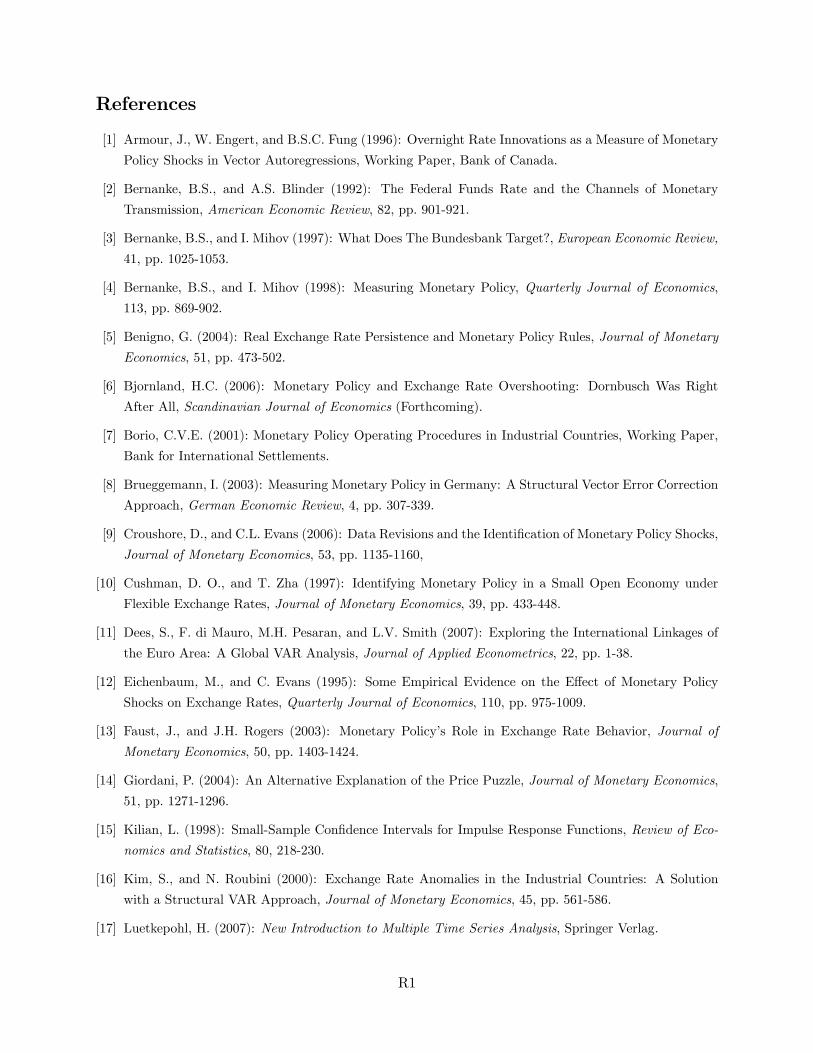
occur immediately, but the impulse response function rather exhibits a hump-shape pattern, the so

called “delayed exchange rate overshooting puzzle”. Furthermore, the empirical evidence appears

to contradict uncovered interest parity (which has been termed the “forward premium puzzle”), and

impulse responses for domestic prices appear to rise rather than fall after a contractionary monetary

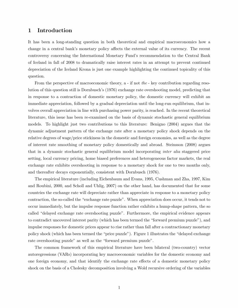
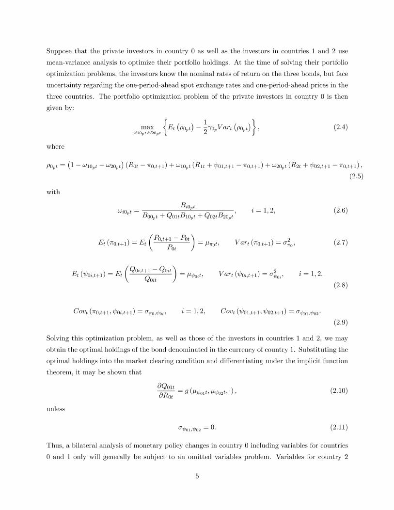
policy shock (which has been termed the “price puzzle”). Figure 1 illustrates the “delayed exchange

rate overshooting puzzle” as well as the “forward premium puzzle”.

The common framework of this empirical literature have been bilateral (two-country) vector

autoregressions (VARs) incorporating key macroeconomic variables for the domestic economy and

one foreign economy, and that identify the exchange rate effects of a domestic monetary policy

shock on the basis of a Cholesky decomposition involving a Wold recursive ordering of the variables

1

contained in the VAR.1

In this paper, we address the question to what extent these previous empirical findings may have

been caused by two issues: (i) Working with bilateral VARs neglects to account for simultaneous

multilateral (multi-country) adjustments of key macroeconomic variables in response to monetary

policy shocks - such multi-country adjustments, however, do seem to be an essential feature of

economies with sizeable trade and financial market linkages. (ii) Imposing short-run restrictions of

the form of Cholesky decompositions tends to be difficult to reconcile with macroeconomic theory,

and does not take advantage of the identifying restrictions implied by long-run relations between the

macroeconomic variables under consideration in the VAR. In this paper, we specify a multi-country

VAR model for a panel of nine industrial economies (Australia, Canada, France, Germany, Italy,

Japan, New Zealand, United Kingdom, and the United States), using monthly data from 1978 to

2006. On the basis of this multi-country specification and exploiting empirically supported long-run

relationships for the identification of monetary policy shocks, we find that U.S. Dollar effective and

bilateral real exchange rates appreciate immediately after a contractionary U.S. monetary policy

shock, and that there is no delayed overshooting. Furthermore, there is no persistent significant

deviation from uncovered interest parity, and the price puzzle is at most weakly present. These

results suggest that a dynamic stochastic general equilibrium model as in Steinsson (2008) actually

is consistent with the data in regards to its implications for the real exchange rate effects of monetary

policy shocks.

The remainder of the paper is structured as follows: In Section 2, we review the empirical models

considered in the previous literature, in particular the benchmark model of Eichenbaum and Evans

(1995), provide a brief theoretical motivation for studying multilateral models, and introduce our

empirical model specification. We discuss the measurement of monetary policy shocks in Section 3.

We provide our empirical results in Section 4, and in Section 5 adduce various comparisons between

results from our empirical model specification and those employed in the previous literature. Finally,

Section 6 concludes.

2 The Empirical Model

2.1 Methodology of Eichenbaum and Evans (1995)

Almost all of the empirical models considered in the previous literature are bilateral (two-country)

vector autoregressions (VARs). We take one of the specifications in Eichenbaum and Evans (1995)

as a benchmark. Eichenbaum and Evans (1995) use such a VAR to model the bilateral relationship

1Recent empirical work employing weaker short-run identification schemes such as sign restrictions, for example

Scholl and Uhlig (2007), argues that the various puzzles are not tied to the identification of VARs using Cholesky

decompositions.

2

for five country pairs: the United States versus France, the United States versus Germany, the

United States versus Italy, the United States versus Japan, and the United States versus the United

Kingdom. For each of these country pairs the seven-variable VAR considered by Eichenbaum and

Evans (1995) is given by

zt = a0 + a1t+

pXs=1

Aszt−s + ut, utiid∼ (0,Ωu) , (2.1)

where

zt =³Yt Pt Y ∗t R∗t FFRt nbrt qt

´0, (2.2)

with Yt denoting U.S. industrial production, Pt the U.S. consumer price index, Y∗t foreign industrial

production, R∗t the foreign short-term interest rate, FFRt the federal funds rate, nbrt the ratio

between U.S. non-borrowed reserves and total reserves, and qt the bilateral real exchange rate. All

variables, except for the interest rates, are in logarithms. The VAR lag order, p, is chosen to be equal

to six for the monthly data sample Eichenbaum and Evans (1995) do work with. The monetary

policy shock is identified using a Cholesky decomposition assuming a Wold causal ordering (this

ordering being as in (2.2)) of the variables, inter alia implying that the Federal Reserve sets the

federal funds rate taking into account the lagged values of all the components of zt as well as the

current values of U.S. industrial production, U.S. prices, foreign industrial production, and the

foreign short-term interest rate.

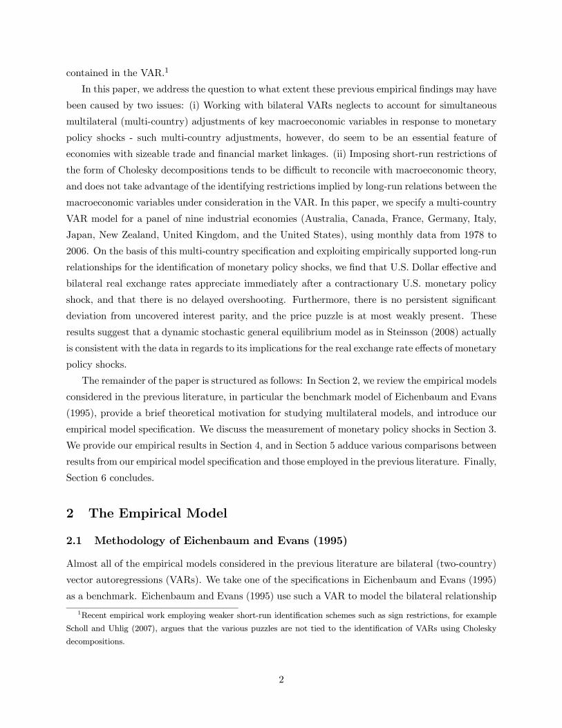
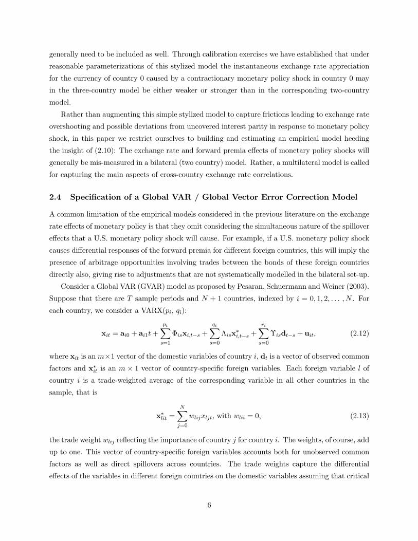
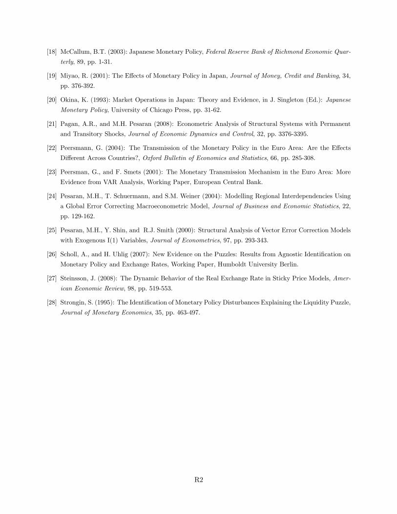
Selecting the United States versus Germany based bilateral VAR of Eichenbaum and Evans

(1995) as one representative example, Figure 2 shows the impulse responses for various key variables

after a U.S. monetary policy shock as obtained by Eichenbaum and Evans (1995).2 In regards to

exchange rate effects, the bilateral exchange rate of the U.S. Dollar relative to the Deutsche Mark

overshoots its long-run level with a delay of about three years, termed the “delayed exchange rate

overshooting puzzle”. The interest rate differential between the federal funds rate and the German

short-term interest rate after the U.S. monetary policy shock exhibits for about 18 months a positive

difference. The (ex post) forward premium, defined as in Eichenbaum and Evans (1995), namely

ξt = −[R∗t −Rt + (Qt+1 −Qt)],

(the ex post excess return for a U.S. investor from investing in U.S. short-term maturity bonds, with

rate of return Rt, relative to investing in short-term maturity German bonds), in response to a U.S.

monetary policy shock deviates substantially from zero for about one year, termed the “forward

premium puzzle”. Finally (though not displayed in Figure 2), Eichenbaum and Evans (1995)

also find that the impulse responses for prices display a positive reaction to the contractionary

2All impulse response standard error bands in this paper are 95% error bands, which were obtained using a

bootstrapping algorithm as in Kilian (1998).

3

U.S. monetary policy shock, rather than following the pattern of a dynamic stochastic general

equilibrium macroeconomic model with price stickiness, namely of initially failing to respond and

after a while beginning to fall.

2.2 Further Recent Empirical Work

Since Eichenbaum and Evans (1995), several papers, including Cushman and Zha (1997), Kim and

Roubini (2000), as well as Faust and Rogers (2003) have explored the robustness of these results to

the identification of the U.S. monetary policy shock. In particular, Faust and Rogers (2003) impose

sign and/or impulse response shape restrictions, and find that the exchange rate impulse response

is sensitive to different short-run restrictions, with no robust conclusion about the timing of the

appreciation peak after a contractionary monetary policy shock being possible. Faust and Rogers

(2003) find the “forward premium puzzle”, on the other hand, to be robust to the sign and/or

impulse response shape restrictions imposed. Scholl and Uhlig (2007) also use sign restrictions, and

find that the “delayed exchange rate overshooting puzzle” remains, and that the “forward premium

puzzle” is robust even without delayed overshooting.

Bjornland (2006) does not use a bilateral VAR. Instead, she includes a trade-weighted foreign

interest rate in the model for the domestic economy, and identifies the monetary policy shock in

a specification that allows for interaction between the central bank’s interest rate policy and its

exchange rate policies. Bjornland (2006) finds that exchange rates display no delayed overshooting,

and that the uncovered interest parity holds for the majority of the five countries she considers in

her sample.

2.3 Multilateral Models: Motivation

In this sub-section we provide a brief theoretical motivation for working with multilateral rather

than bilateral models when analyzing the exchange rate effects of monetary policy shocks. The

model we will in this sub-section consider is very stylized, focussing on the instantaneous exchange

rate effects of monetary policy shocks rather than attempting to construct a fully specified dy-

namic stochastic general equilibrium, multi-country model capturing all the variables entering our

subsequent empirical analysis.

Consider a three-country model. For simplicity, suppose that there are only three types of

financial assets, bonds of maturity one period denominated in the currencies of country 0, country

1, and country 2, respectively. As we will consider the exchange rate effects of changes in monetary

policy in country 0 only, for country 0 only we distinguish between private investors and monetary

authorities. We have the following period t equilibrium conditions for the three bonds:

Bi0gt +Bi0pt +Bi1t +Bi2t = 0, i = 0, 1, 2. (2.3)

4

Suppose that the private investors in country 0 as well as the investors in countries 1 and 2 use

mean-variance analysis to optimize their portfolio holdings. At the time of solving their portfolio

optimization problems, the investors know the nominal rates of return on the three bonds, but face

uncertainty regarding the one-period-ahead spot exchange rates and one-period-ahead prices in the

three countries. The portfolio optimization problem of the private investors in country 0 is then

given by:

maxω10pt,ω20pt

½Et

¡ρ0pt

¢− 12γ0pV art

¡ρ0pt

¢¾, (2.4)

where

ρ0pt =¡1− ω10pt − ω20pt

¢(R0t − π0,t+1) + ω10pt (R1t + ψ01,t+1 − π0,t+1) + ω20pt (R2t + ψ02,t+1 − π0,t+1) ,

(2.5)

with

ωi0pt =Bi0pt

B00pt +Q01tB10pt +Q02tB20pt, i = 1, 2, (2.6)

Et (π0,t+1) = Et

µP0,t+1 − P0t

P0t

¶= μπ0t, V art (π0,t+1) = σ2π0 , (2.7)

Et (ψ0i,t+1) = Et

µQ0i,t+1 −Q0it

Q0it

¶= μψ0it, V art (ψ0i,t+1) = σ2ψ0i , i = 1, 2.

(2.8)

Covt (π0,t+1, ψ0i,t+1) = σπ0,ψ0i , i = 1, 2, Covt (ψ01,t+1, ψ02,t+1) = σψ01,ψ02 .

(2.9)

Solving this optimization problem, as well as those of the investors in countries 1 and 2, we may

obtain the optimal holdings of the bond denominated in the currency of country 1. Substituting the

optimal holdings into the market clearing condition and differentiating under the implicit function

theorem, it may be shown that

∂Q01t∂R0t

= g (μψ01t, μψ02t, ·) , (2.10)

unless

σψ01,ψ02 = 0. (2.11)

Thus, a bilateral analysis of monetary policy changes in country 0 including variables for countries

0 and 1 only will generally be subject to an omitted variables problem. Variables for country 2

5

generally need to be included as well. Through calibration exercises we have established that under

reasonable parameterizations of this stylized model the instantaneous exchange rate appreciation

for the currency of country 0 caused by a contractionary monetary policy shock in country 0 may

in the three-country model be either weaker or stronger than in the corresponding two-country

model.

Rather than augmenting this simple stylized model to capture frictions leading to exchange rate

overshooting and possible deviations from uncovered interest parity in response to monetary policy

shock, in this paper we restrict ourselves to building and estimating an empirical model heeding

the insight of (2.10): The exchange rate and forward premia effects of monetary policy shocks will

generally be mis-measured in a bilateral (two country) model. Rather, a multilateral model is called

for capturing the main aspects of cross-country exchange rate correlations.

2.4 Specification of a Global VAR / Global Vector Error Correction Model

A common limitation of the empirical models considered in the previous literature on the exchange

rate effects of monetary policy is that they omit considering the simultaneous nature of the spillover

effects that a U.S. monetary policy shock will cause. For example, if a U.S. monetary policy shock

causes differential responses of the forward premia for different foreign countries, this will imply the

presence of arbitrage opportunities involving trades between the bonds of these foreign countries

directly also, giving rise to adjustments that are not systematically modelled in the bilateral set-up.

Consider a Global VAR (GVAR) model as proposed by Pesaran, Schuermann andWeiner (2003).

Suppose that there are T sample periods and N + 1 countries, indexed by i = 0, 1, 2, . . . , N . For

each country, we consider a VARX(pi, qi):

xit = ai0 + ai1t+

piXs=1

Φisxi,t−s +qiXs=0

Λisx∗i,t−s +

riXs=0

Υisdt−s + uit, (2.12)

where xit is anm×1 vector of the domestic variables of country i, dt is a vector of observed commonfactors and x∗it is an m × 1 vector of country-specific foreign variables. Each foreign variable l ofcountry i is a trade-weighted average of the corresponding variable in all other countries in the

sample, that is

x∗lit =NXj=0

wlijxljt, with wlii = 0, (2.13)

the trade weight wlij reflecting the importance of country j for country i. The weights, of course, add

up to one. This vector of country-specific foreign variables accounts both for unobserved common

factors as well as direct spillovers across countries. The trade weights capture the differential

effects of the variables in different foreign countries on the domestic variables assuming that critical

6

to the magnitude of spillovers is the magnitude of trade.3 The country-specific foreign variables

and the observed common factors are treated as weakly exogenous (which is, of course, a testable

restriction).

Further, in order to distinguish short-run and long-run dynamics in the presence of both tempo-

rary and permanent shocks, we re-write Equation (2.12) in error-correction format (Global Vector

Error Correction Model, GVECM) as:

∆xit = ci0 + ci1t+Πiezi,t−1 + p−1Xs=1

Ψis∆zi,t−s + Γi∆x∗it +riXs=0

Θi∆dt + uit, (2.14)

where ezit = ³x0it, x∗0it , d0t´0 , zit = ³x0it, x∗0it´0, and p = max pi, qifor all i. The matrix Πi may bedecomposed as Πi = αiβ

0i, where βi is the matrix of cointegrating relations.

While under weak exogeneity of the country-specific foreign variables and the observed common

factors one may estimate Equations (2.12) and (2.14) on a country-by-country basis, it is still

necessary to obtain the implied global solution for xt =³x00t, x01t, . . . , x0Nt

´0. To obtain the

global solution in levels form, note that Equation (2.12) can also be re-written as

Aizit = ai0 + ai1 · t+pX

s=1

Bsizi,t−s +riXs=0

Υisdt−s + uit. (2.15)

From Equation (2.13), zit = Wixt for some matrix of weights Wi. By stacking Equation (2.15)

across i, the resultant system can be re-written as⎛⎜⎜⎜⎜⎜⎝A0W0

A1W1

...

ANWN

⎞⎟⎟⎟⎟⎟⎠xt| z

G(k×k)

= a0 + a1 · t+

⎛⎜⎜⎜⎜⎜⎝B10W0

B12W1

...

B1NWN

⎞⎟⎟⎟⎟⎟⎠| z

H1(k×k)

xt−1 + . . .+

⎛⎜⎜⎜⎜⎜⎝Bp0W0

Bp2W1

...

BpNWN

⎞⎟⎟⎟⎟⎟⎠| z

xt−p

Hp(k×k)

+rX

s=0

Υsdt−s + ut,

(2.16)

with k being the number of the all domestic variables for all countries and r = max (ri). The

matrix G can in general expected to be of full rank, implying that the global solution in levels form

is given by

Xt = G−1a0 + G−1a1t +

pXs=1

G−1Hsxt−s + G−1ut. (2.17)

This in fact is a VAR for the domestic variables in all sample countries, through which their

impulse responses to a shock on any of these variables can be obtained. The key advantage of

3To capture a separate financial market channel of spillovers, one would like to use financial capital flow based

weights also, at least for financial market variables. As such bilateral financial capital flow based weights are not

broadly available, we restrict ourselves to trade weights here.

7

the GVAR/GVECM framework is that one can estimate Equation (2.17) indirectly on a country-

by-country basis, allowing for the consideration of a much larger number of countries and a much

richer set of country-specific model specifications than would ever be feasible when attempting to

estimate Equation (2.17) directly.

2.5 Model Variables and Data

We consider the sample period from January 1978 to December 2006 for nine industrial countries:

Australia, Canada, France, Germany, Italy, Japan, New Zealand, the United Kingdom, and the

United States. The vector of domestic variables for each country is given by:

xit =³Yit Pit Rm

it Rit Qit

´0, (2.18)

where

Yit: logarithm of industrial production,

Pit: logarithm of consumer price index (with base year 2000),

Rmit : monetary policy indicator (in fractions),

Rit: short-term interest rate (typically a three-months treasury-bill type rate, in fractions),

Qit: trade weighted effective nominal exchange rate.

The corresponding country-specific foreign variables are given by:

x∗it =³Y ∗it P ∗it R∗it Q∗it

´0. (2.19)

We do not construct country-specific foreign variables for the monetary policy indicator, since the

indicator for each country reflects different variables. See Section ?? for a detailed discussion of the

monetary policy indicators. The weights used for the construction of the foreign variables and the

effective exchange rates are average trade weights based on a middle period in the sample (namely,

from January 1991 to December 1993).

3 Measuring Monetary Policy Shocks

3.1 Monetary Policy Indicator

Turn to the issue of measuring the monetary policy shock. First, we need to choose the indica-

tors that for each country seem to best measure the monetary policy stance. It has been widely

recognized in the literature that money stocks do not represent satisfactory measures of the mone-

tary policy stance, as changes of the money stock involve various non-policy influences and reflect

both changes of money demand and money supply.4 Hence we focus on other variables such as

short-term interest rates and reserve ratios. Let us briefly discuss our choices for each country.

4For example, Reichenstein (1987), Leeper and Gordon (1992), Strongin (1995), and Bernanke and Mihov (1998).

8

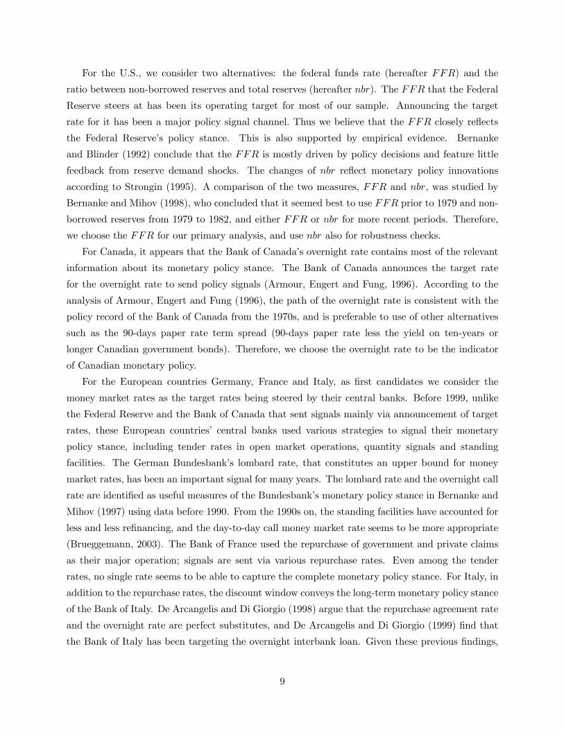
For the U.S., we consider two alternatives: the federal funds rate (hereafter FFR) and the

ratio between non-borrowed reserves and total reserves (hereafter nbr). The FFR that the Federal

Reserve steers at has been its operating target for most of our sample. Announcing the target

rate for it has been a major policy signal channel. Thus we believe that the FFR closely reflects

the Federal Reserve’s policy stance. This is also supported by empirical evidence. Bernanke

and Blinder (1992) conclude that the FFR is mostly driven by policy decisions and feature little

feedback from reserve demand shocks. The changes of nbr reflect monetary policy innovations

according to Strongin (1995). A comparison of the two measures, FFR and nbr, was studied by

Bernanke and Mihov (1998), who concluded that it seemed best to use FFR prior to 1979 and non-

borrowed reserves from 1979 to 1982, and either FFR or nbr for more recent periods. Therefore,

we choose the FFR for our primary analysis, and use nbr also for robustness checks.

For Canada, it appears that the Bank of Canada’s overnight rate contains most of the relevant

information about its monetary policy stance. The Bank of Canada announces the target rate

for the overnight rate to send policy signals (Armour, Engert and Fung, 1996). According to the

analysis of Armour, Engert and Fung (1996), the path of the overnight rate is consistent with the

policy record of the Bank of Canada from the 1970s, and is preferable to use of other alternatives

such as the 90-days paper rate term spread (90-days paper rate less the yield on ten-years or

longer Canadian government bonds). Therefore, we choose the overnight rate to be the indicator

of Canadian monetary policy.

For the European countries Germany, France and Italy, as first candidates we consider the

money market rates as the target rates being steered by their central banks. Before 1999, unlike

the Federal Reserve and the Bank of Canada that sent signals mainly via announcement of target

rates, these European countries’ central banks used various strategies to signal their monetary

policy stance, including tender rates in open market operations, quantity signals and standing

facilities. The German Bundesbank’s lombard rate, that constitutes an upper bound for money

market rates, has been an important signal for many years. The lombard rate and the overnight call

rate are identified as useful measures of the Bundesbank’s monetary policy stance in Bernanke and

Mihov (1997) using data before 1990. From the 1990s on, the standing facilities have accounted for

less and less refinancing, and the day-to-day call money market rate seems to be more appropriate

(Brueggemann, 2003). The Bank of France used the repurchase of government and private claims

as their major operation; signals are sent via various repurchase rates. Even among the tender

rates, no single rate seems to be able to capture the complete monetary policy stance. For Italy, in

addition to the repurchase rates, the discount window conveys the long-term monetary policy stance

of the Bank of Italy. De Arcangelis and Di Giorgio (1998) argue that the repurchase agreement rate

and the overnight rate are perfect substitutes, and De Arcangelis and Di Giorgio (1999) find that

the Bank of Italy has been targeting the overnight interbank loan. Given these previous findings,

9

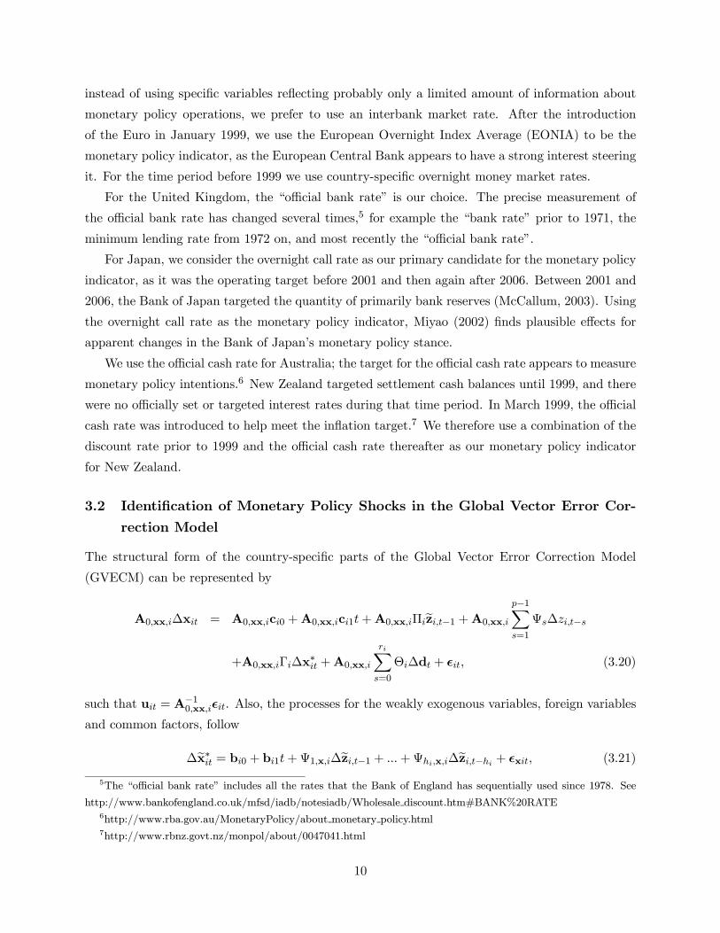
instead of using specific variables reflecting probably only a limited amount of information about

monetary policy operations, we prefer to use an interbank market rate. After the introduction

of the Euro in January 1999, we use the European Overnight Index Average (EONIA) to be the

monetary policy indicator, as the European Central Bank appears to have a strong interest steering

it. For the time period before 1999 we use country-specific overnight money market rates.

For the United Kingdom, the “official bank rate” is our choice. The precise measurement of

the official bank rate has changed several times,5 for example the “bank rate” prior to 1971, the

minimum lending rate from 1972 on, and most recently the “official bank rate”.

For Japan, we consider the overnight call rate as our primary candidate for the monetary policy

indicator, as it was the operating target before 2001 and then again after 2006. Between 2001 and

2006, the Bank of Japan targeted the quantity of primarily bank reserves (McCallum, 2003). Using

the overnight call rate as the monetary policy indicator, Miyao (2002) finds plausible effects for

apparent changes in the Bank of Japan’s monetary policy stance.

We use the official cash rate for Australia; the target for the official cash rate appears to measure

monetary policy intentions.6 New Zealand targeted settlement cash balances until 1999, and there

were no officially set or targeted interest rates during that time period. In March 1999, the official

cash rate was introduced to help meet the inflation target.7 We therefore use a combination of the

discount rate prior to 1999 and the official cash rate thereafter as our monetary policy indicator

for New Zealand.

3.2 Identification of Monetary Policy Shocks in the Global Vector Error Cor-

rection Model

The structural form of the country-specific parts of the Global Vector Error Correction Model

(GVECM) can be represented by

A0,xx,i∆xit = A0,xx,ici0 +A0,xx,ici1t+A0,xx,iΠiezi,t−1 +A0,xx,i p−1Xs=1

Ψs∆zi,t−s

+A0,xx,iΓi∆x∗it +A0,xx,i

riXs=0

Θi∆dt + ²it, (3.20)

such that uit = A−10,xx,i²it. Also, the processes for the weakly exogenous variables, foreign variables

and common factors, follow

∆ex∗it = bi0 + bi1t+Ψ1,x,i∆ezi,t−1 + ...+Ψhi,x,i∆ezi,t−hi + ²xit, (3.21)

5The “official bank rate” includes all the rates that the Bank of England has sequentially used since 1978. See

http://www.bankofengland.co.uk/mfsd/iadb/notesiadb/Wholesale discount.htm#BANK%20RATE6http://www.rba.gov.au/MonetaryPolicy/about monetary policy.html7http://www.rbnz.govt.nz/monpol/about/0047041.html

10

where ex∗it = ³ x∗0it , d0t´0, and hi = maxp, ri.

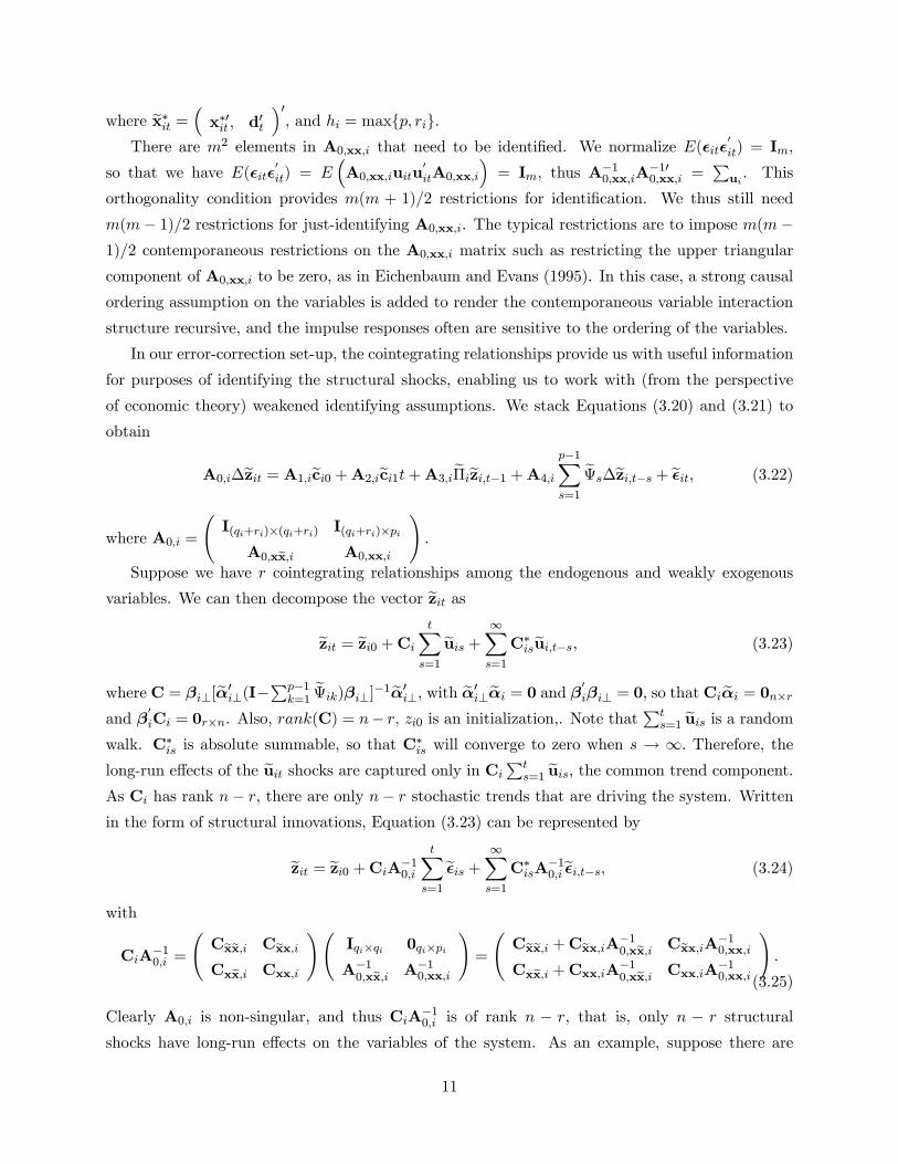
There are m2 elements in A0,xx,i that need to be identified. We normalize E(²it²0it) = Im,

so that we have E(²it²0it) = E

³A0,xx,iuitu

0itA0,xx,i

´= Im, thus A

−10,xx,iA

−100,xx,i =

Pui. This

orthogonality condition provides m(m + 1)/2 restrictions for identification. We thus still need

m(m− 1)/2 restrictions for just-identifying A0,xx,i. The typical restrictions are to impose m(m−1)/2 contemporaneous restrictions on the A0,xx,i matrix such as restricting the upper triangular

component of A0,xx,i to be zero, as in Eichenbaum and Evans (1995). In this case, a strong causal

ordering assumption on the variables is added to render the contemporaneous variable interaction

structure recursive, and the impulse responses often are sensitive to the ordering of the variables.

In our error-correction set-up, the cointegrating relationships provide us with useful information

for purposes of identifying the structural shocks, enabling us to work with (from the perspective

of economic theory) weakened identifying assumptions. We stack Equations (3.20) and (3.21) to

obtain

A0,i∆ezit = A1,ieci0 +A2,ieci1t+A3,ieΠiezi,t−1 +A4,i p−1Xs=1

eΨs∆ezi,t−s + e²it, (3.22)

where A0,i =

ÃI(qi+ri)×(qi+ri) I(qi+ri)×pi

A0,xx,i A0,xx,i

!.

Suppose we have r cointegrating relationships among the endogenous and weakly exogenous

variables. We can then decompose the vector ezit asezit = ezi0 +Ci

tXs=1

euis + ∞Xs=1

C∗iseui,t−s, (3.23)

where C = βi⊥[eα0i⊥(I−Pp−1k=1

eΨik)βi⊥]−1eα0i⊥, with eα0i⊥eαi = 0 and β0iβi⊥ = 0, so that Cieαi = 0n×r

and β0iCi = 0r×n. Also, rank(C) = n− r, zi0 is an initialization,. Note that

Pts=1 euis is a random

walk. C∗is is absolute summable, so that C∗is will converge to zero when s → ∞. Therefore, the

long-run effects of the euit shocks are captured only in CiPt

s=1 euis, the common trend component.As Ci has rank n− r, there are only n− r stochastic trends that are driving the system. Written

in the form of structural innovations, Equation (3.23) can be represented by

ezit = ezi0 +CiA−10,i

tXs=1

e²is + ∞Xs=1

C∗isA−10,ie²i,t−s, (3.24)

with

CiA−10,i =

ÃCxx,i Cxx,i

Cxx,i Cxx,i

!ÃIqi×qi 0qi×piA−10,xx,i A−10,xx,i

!=

ÃCxx,i +Cxx,iA

−10,xx,i Cxx,iA

−10,xx,i

Cxx,i +Cxx,iA−10,xx,i Cxx,iA

−10,xx,i

!.

(3.25)

Clearly A0,i is non-singular, and thus CiA−10,i is of rank n − r, that is, only n − r structural

shocks have long-run effects on the variables of the system. As an example, suppose there are

11

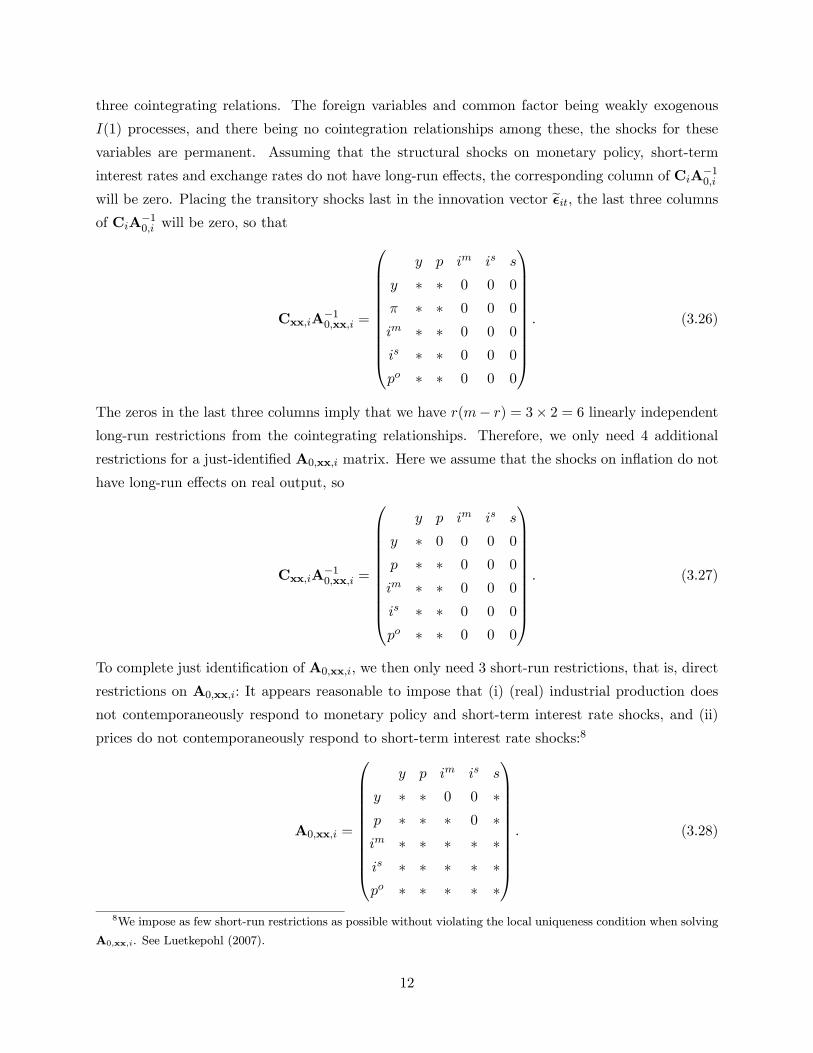
three cointegrating relations. The foreign variables and common factor being weakly exogenous

I(1) processes, and there being no cointegration relationships among these, the shocks for these

variables are permanent. Assuming that the structural shocks on monetary policy, short-term

interest rates and exchange rates do not have long-run effects, the corresponding column of CiA−10,i

will be zero. Placing the transitory shocks last in the innovation vector e²it, the last three columnsof CiA

−10,i will be zero, so that

Cxx,iA−10,xx,i =

⎛⎜⎜⎜⎜⎜⎜⎜⎜⎜⎜⎝

y p im is s

y ∗ ∗ 0 0 0

π ∗ ∗ 0 0 0

im ∗ ∗ 0 0 0

is ∗ ∗ 0 0 0

po ∗ ∗ 0 0 0

⎞⎟⎟⎟⎟⎟⎟⎟⎟⎟⎟⎠. (3.26)

The zeros in the last three columns imply that we have r(m− r) = 3× 2 = 6 linearly independentlong-run restrictions from the cointegrating relationships. Therefore, we only need 4 additional

restrictions for a just-identified A0,xx,i matrix. Here we assume that the shocks on inflation do not

have long-run effects on real output, so

Cxx,iA−10,xx,i =

⎛⎜⎜⎜⎜⎜⎜⎜⎜⎜⎜⎝

y p im is s

y ∗ 0 0 0 0

p ∗ ∗ 0 0 0

im ∗ ∗ 0 0 0

is ∗ ∗ 0 0 0

po ∗ ∗ 0 0 0

⎞⎟⎟⎟⎟⎟⎟⎟⎟⎟⎟⎠. (3.27)

To complete just identification of A0,xx,i, we then only need 3 short-run restrictions, that is, direct

restrictions on A0,xx,i: It appears reasonable to impose that (i) (real) industrial production does

not contemporaneously respond to monetary policy and short-term interest rate shocks, and (ii)

prices do not contemporaneously respond to short-term interest rate shocks:8

A0,xx,i =

⎛⎜⎜⎜⎜⎜⎜⎜⎜⎜⎜⎝

y p im is s

y ∗ ∗ 0 0 ∗p ∗ ∗ ∗ 0 ∗im ∗ ∗ ∗ ∗ ∗is ∗ ∗ ∗ ∗ ∗po ∗ ∗ ∗ ∗ ∗

⎞⎟⎟⎟⎟⎟⎟⎟⎟⎟⎟⎠. (3.28)

8We impose as few short-run restrictions as possible without violating the local uniqueness condition when solving

A0,xx,i. See Luetkepohl (2007).

12

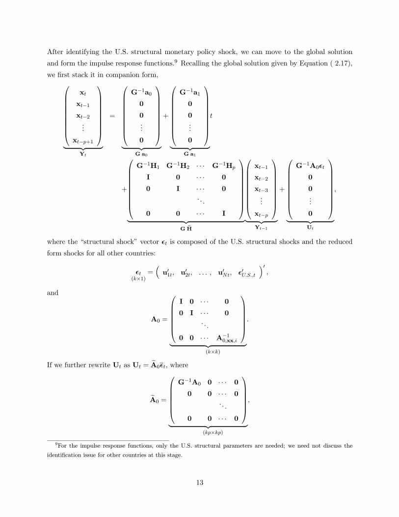
After identifying the U.S. structural monetary policy shock, we can move to the global solution

and form the impulse response functions.9 Recalling the global solution given by Equation ( 2.17),

we first stack it in companion form,⎛⎜⎜⎜⎜⎜⎜⎜⎜⎝

xt

xt−1xt−2...

xt−p+1

⎞⎟⎟⎟⎟⎟⎟⎟⎟⎠| z

Yt

=

⎛⎜⎜⎜⎜⎜⎜⎜⎜⎝

G−1a00

0...

0

⎞⎟⎟⎟⎟⎟⎟⎟⎟⎠| z

G a0

+

⎛⎜⎜⎜⎜⎜⎜⎜⎜⎝

G−1a10

0...

0

⎞⎟⎟⎟⎟⎟⎟⎟⎟⎠| z

G a1

t

+

⎛⎜⎜⎜⎜⎜⎜⎜⎜⎝

G−1H1 G−1H2 · · · G−1Hp

I 0 · · · 0

0 I · · · 0. . .

0 0 · · · I

⎞⎟⎟⎟⎟⎟⎟⎟⎟⎠| z

GH

⎛⎜⎜⎜⎜⎜⎜⎜⎜⎝

xt−1xt−2xt−3...

xt−p

⎞⎟⎟⎟⎟⎟⎟⎟⎟⎠| z

Yt−1

+

⎛⎜⎜⎜⎜⎜⎜⎜⎜⎝

G−1A0²t0

0...

0

⎞⎟⎟⎟⎟⎟⎟⎟⎟⎠| z

Ut

,

where the “structural shock” vector ²t is composed of the U.S. structural shocks and the reduced

form shocks for all other countries:

²t(k×1)

=³u01t, u02t, . . . , u0Nt, ²0U.S.,t

´0,

and

A0 =

⎛⎜⎜⎜⎜⎜⎝I 0 · · · 0

0 I · · · 0. . .

0 0 · · · A−10,xx,i

⎞⎟⎟⎟⎟⎟⎠| z

(k×k)

.

If we further rewrite Ut as Ut = eA0²t, whereeA0 =

⎛⎜⎜⎜⎜⎜⎝G−1A0 0 · · · 0

0 0 · · · 0. . .

0 0 · · · 0

⎞⎟⎟⎟⎟⎟⎠| z

(kp×kp)

,

9For the impulse response functions, only the U.S. structural parameters are needed; we need not discuss the

identification issue for other countries at this stage.

13

and ²t =³²0t, 0, . . . , 0

´0, then the s-period ahead impulse response for a U.S. monetary

policy shock is computed as

IRs (Yt) =³G eH´sG−1E ¡ut ¯²Rm

US ,t= κ

¢,

where

E(ut¯²Rm

US ,t= κ) = E(eA0²t ¯²Rm

US ,t= κ)

= eA0E(²t ¯²RmUS ,t

= κ)

= eA0 Cov(²t)eiV ar(²Rm

US ,t)κ,

with ei being the selection vector detailing the location of the U.S. monetary policy shock in the

vector ²t. We should note that identify all the shocks in the global solution given by Equation (2.17)

would result in our empirical study of having to impose more than 2,000 parameter restrictions. We

therefore choose to identify the U.S. monetary policy shock in the U.S. equation of the GVECM.

Doing so, we do not impose the restriction that the U.S. structural monetary policy shock would be

uncorrelated with shocks in other countries and do not impose any zero short-run impact restrictions

for the structural shocks across countries. On this count, we let the data speak freely.

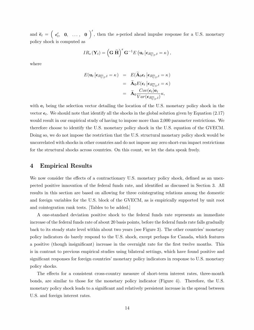
4 Empirical Results

We now consider the effects of a contractionary U.S. monetary policy shock, defined as an unex-

pected positive innovation of the federal funds rate, and identified as discussed in Section 3. All

results in this section are based on allowing for three cointegrating relations among the domestic

and foreign variables for the U.S. block of the GVECM, as is empirically supported by unit root

and cointegration rank tests. [Tables to be added.]

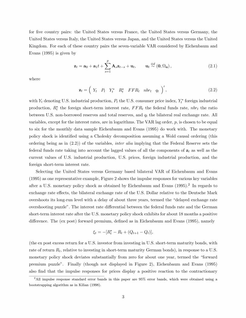
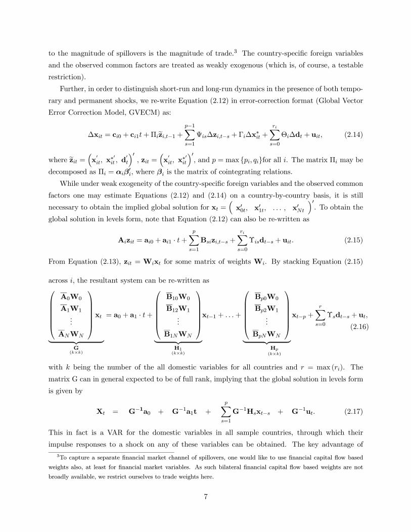
A one-standard deviation positive shock to the federal funds rate represents an immediate

increase of the federal funds rate of about 20 basis points, before the federal funds rate falls gradually

back to its steady state level within about two years (see Figure 3). The other countries’ monetary

policy indicators do barely respond to the U.S. shock, except perhaps for Canada, which features

a positive (though insignificant) increase in the overnight rate for the first twelve months. This

is in contrast to previous empirical studies using bilateral settings, which have found positive and

significant responses for foreign countries’ monetary policy indicators in response to U.S. monetary

policy shocks.

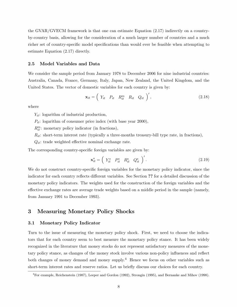
The effects for a consistent cross-country measure of short-term interest rates, three-month

bonds, are similar to those for the monetary policy indicator (Figure 4). Therefore, the U.S.

monetary policy shock leads to a significant and relatively persistent increase in the spread between

U.S. and foreign interest rates.

14

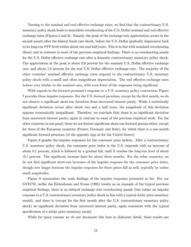
Turning to the nominal and real effective exchange rates, we find that the contractionary U.S.

monetary policy shock leads to immediate overshooting of the U.S. Dollar nominal and real effective

exchange rates (Figures 5 and 6). Namely, the peak of the exchange rate appreciation occurs in the

second month after the federal funds rate shock, before the U.S. Dollar gradually depreciates back

to its long-run PPP level within about one and half years. This is in line with standard overshooting

theory and in contrast to most of the previous empirical findings. There is no overshooting puzzle

for the U.S. Dollar effective exchange rate after a domestic contractionary monetary policy shock.

The appreciation at the peak is about 0.9 percent for the nominal U.S. Dollar effective exchange

rate, and about 1.0 percent for the real U.S. Dollar effective exchange rate. The majority of the

other countries’ nominal effective exchange rates respond to the contractionary U.S. monetary

policy shock with a small and often insignificant depreciation. The real effective exchange rates

behave very similar to the nominal ones, with even fewer of the responses being significant.

With regards to the forward premium’s response to a U.S. monetary policy contraction, Figure

7 provides these impulse responses. For the U.S. forward premium, except for the first month, we do

not observe a significant short-run deviation from uncovered interest parity. While a statistically

significant deviation occurs after about two and a half years, the magnitude of this deviation

appears economically insignificant. Therefore, we conclude that there is no significant deviation

from uncovered interest parity, again in contrast to most of the previous empirical work. For the

other countries in our panel, these do not feature significant short-run forward premia either, except

for three of the European countries (France, Germany and Italy), for which there is a one-month

significant forward premium (of the opposite sign as for the United States).

Figure 8 graphs the impulse responses for the consumer price indices. After a contractionary

U.S. monetary policy shock, the consumer price index in the U.S. responds with an increase of

about 0.1 percent, which is followed by a gradual fall, until it reaches the long-run level of about

-0.1 percent. The significant increase lasts for about three months. For the other countries, we

do not find significant short-run increases of the impulse response for the consumer price index,

though over longer horizons the impulse responses for these prices fall as well, typically by rather

small magnitudes.

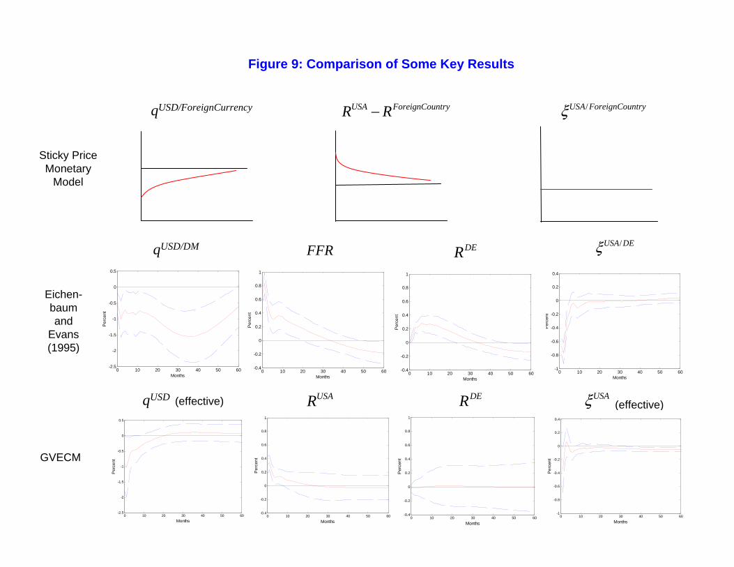
Figure 9 summarizes the main findings of the impulse responses presented so far: For our

GVECM, unlike the Eichenbaum and Evans (1995) results as an example of the typical previous

empirical findings, there is no delayed exchange rate overshooting puzzle (but rather an impulse

response to a U.S. contractionary monetary policy shock in line with a typical sticky price monetary

model), and there is (except for the first month after the U.S. contractionary monetary policy

shock) no significant deviation from uncovered interest parity, again consistent with the typical

specification of a sticky price monetary model.

While for space reasons we do not document this here in elaborate detail, these results are

15

robust to considerations such as modification of our lag length selection criteria as well as the

addition of dummy variables to account for the monetary policy change for some of the European

countries in 1999, and to account for German re-unification in 1990. The results are furthermore

robust to using a broader commodity price index (rather than oil prices) as common factor in the

GVAR / GVECM.

Finally, as can be seen from Figure 10, the GVAR / GVECM based results also do not indicate a

significant reaction of either the bilateral or effective real U.S. Dollar exchange rate to contractionary

monetary policy shocks in countries other than the United States.

5 Model Comparisons and Counterfactual Analysis

Clearly, the Eichenbaum and Evans (1995) specification and our GVECM specification differ beyond

considering bilateral (two country) versus multilateral (multi country) settings in several other

aspects also:

(i) data sets: relative to Eichenbaum and Evans (1995), we have an extended data set available;

(ii) variable specification: our GVECM includes a larger number of foreign variables than accounted

for by Eichenbaum and Evans (1995);

(iii) cointegrating relations: Eichenbaum and Evans (1995) use a level VAR, while our GVECM

imposes restrictions implied by empirically supported cointegrating relations;

(iv) monetary policy shock identification: our GVECM exploits a combination of long- and short-

run restrictions for identification purposes, whereas Eichenbaum and Evans (1995) identify mon-

etary policy shocks based on short-run restrictions imposing a recursive ordering of the model

variables (the Cholesky decomposition).

Therefore, in order to explore the reasons underlying the remarkable differences between our

empirical findings and those of Eichenbaum and Evans (1995), we conduct a step-by-step “coun-

terfactual analysis”.

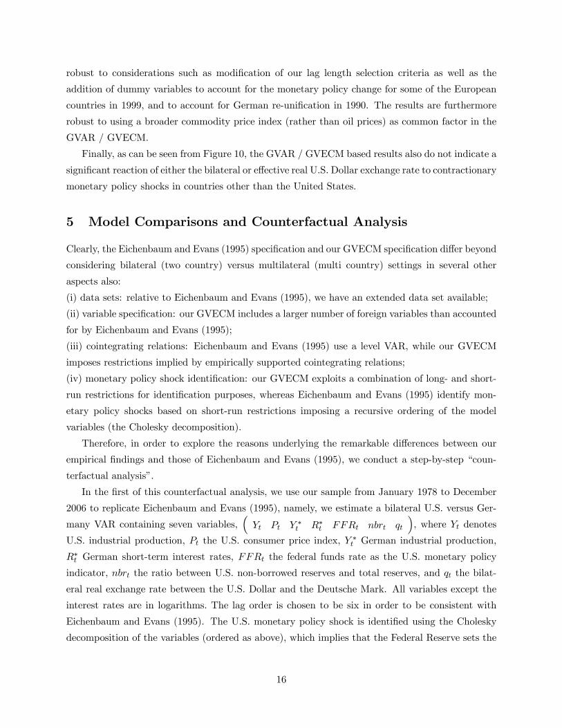
In the first of this counterfactual analysis, we use our sample from January 1978 to December

2006 to replicate Eichenbaum and Evans (1995), namely, we estimate a bilateral U.S. versus Ger-

many VAR containing seven variables,³Yt Pt Y ∗t R∗t FFRt nbrt qt

´, where Yt denotes

U.S. industrial production, Pt the U.S. consumer price index, Y∗t German industrial production,

R∗t German short-term interest rates, FFRt the federal funds rate as the U.S. monetary policy

indicator, nbrt the ratio between U.S. non-borrowed reserves and total reserves, and qt the bilat-

eral real exchange rate between the U.S. Dollar and the Deutsche Mark. All variables except the

interest rates are in logarithms. The lag order is chosen to be six in order to be consistent with

Eichenbaum and Evans (1995). The U.S. monetary policy shock is identified using the Cholesky

decomposition of the variables (ordered as above), which implies that the Federal Reserve sets the

16

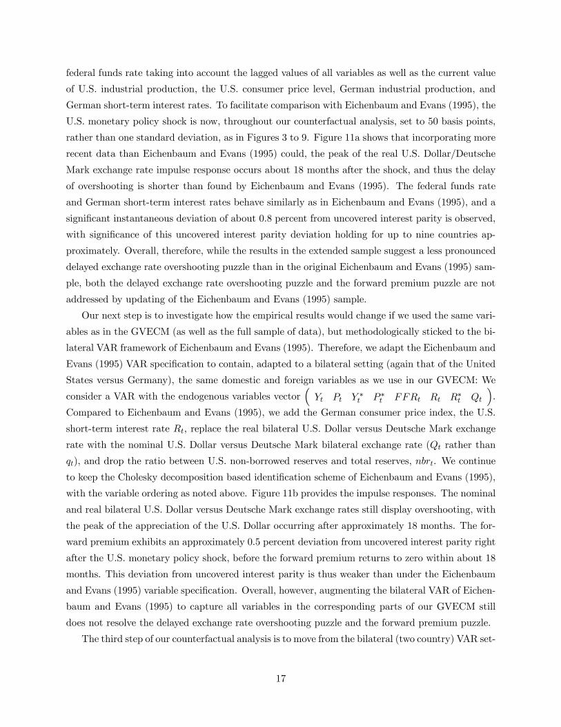
federal funds rate taking into account the lagged values of all variables as well as the current value

of U.S. industrial production, the U.S. consumer price level, German industrial production, and

German short-term interest rates. To facilitate comparison with Eichenbaum and Evans (1995), the

U.S. monetary policy shock is now, throughout our counterfactual analysis, set to 50 basis points,

rather than one standard deviation, as in Figures 3 to 9. Figure 11a shows that incorporating more

recent data than Eichenbaum and Evans (1995) could, the peak of the real U.S. Dollar/Deutsche

Mark exchange rate impulse response occurs about 18 months after the shock, and thus the delay

of overshooting is shorter than found by Eichenbaum and Evans (1995). The federal funds rate

and German short-term interest rates behave similarly as in Eichenbaum and Evans (1995), and a

significant instantaneous deviation of about 0.8 percent from uncovered interest parity is observed,

with significance of this uncovered interest parity deviation holding for up to nine countries ap-

proximately. Overall, therefore, while the results in the extended sample suggest a less pronounced

delayed exchange rate overshooting puzzle than in the original Eichenbaum and Evans (1995) sam-

ple, both the delayed exchange rate overshooting puzzle and the forward premium puzzle are not

addressed by updating of the Eichenbaum and Evans (1995) sample.

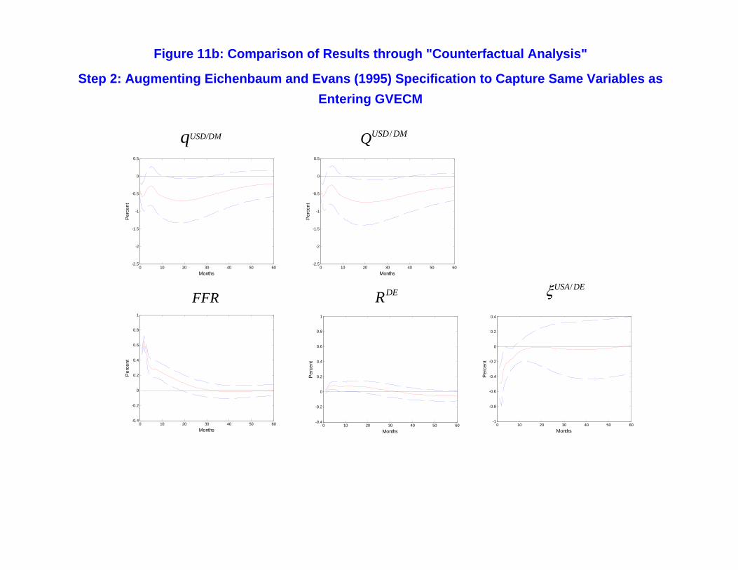
Our next step is to investigate how the empirical results would change if we used the same vari-

ables as in the GVECM (as well as the full sample of data), but methodologically sticked to the bi-

lateral VAR framework of Eichenbaum and Evans (1995). Therefore, we adapt the Eichenbaum and

Evans (1995) VAR specification to contain, adapted to a bilateral setting (again that of the United

States versus Germany), the same domestic and foreign variables as we use in our GVECM: We

consider a VAR with the endogenous variables vector³Yt Pt Y ∗t P ∗t FFRt Rt R∗t Qt

´.

Compared to Eichenbaum and Evans (1995), we add the German consumer price index, the U.S.

short-term interest rate Rt, replace the real bilateral U.S. Dollar versus Deutsche Mark exchange

rate with the nominal U.S. Dollar versus Deutsche Mark bilateral exchange rate (Qt rather than

qt), and drop the ratio between U.S. non-borrowed reserves and total reserves, nbrt. We continue

to keep the Cholesky decomposition based identification scheme of Eichenbaum and Evans (1995),

with the variable ordering as noted above. Figure 11b provides the impulse responses. The nominal

and real bilateral U.S. Dollar versus Deutsche Mark exchange rates still display overshooting, with

the peak of the appreciation of the U.S. Dollar occurring after approximately 18 months. The for-

ward premium exhibits an approximately 0.5 percent deviation from uncovered interest parity right

after the U.S. monetary policy shock, before the forward premium returns to zero within about 18

months. This deviation from uncovered interest parity is thus weaker than under the Eichenbaum

and Evans (1995) variable specification. Overall, however, augmenting the bilateral VAR of Eichen-

baum and Evans (1995) to capture all variables in the corresponding parts of our GVECM still

does not resolve the delayed exchange rate overshooting puzzle and the forward premium puzzle.

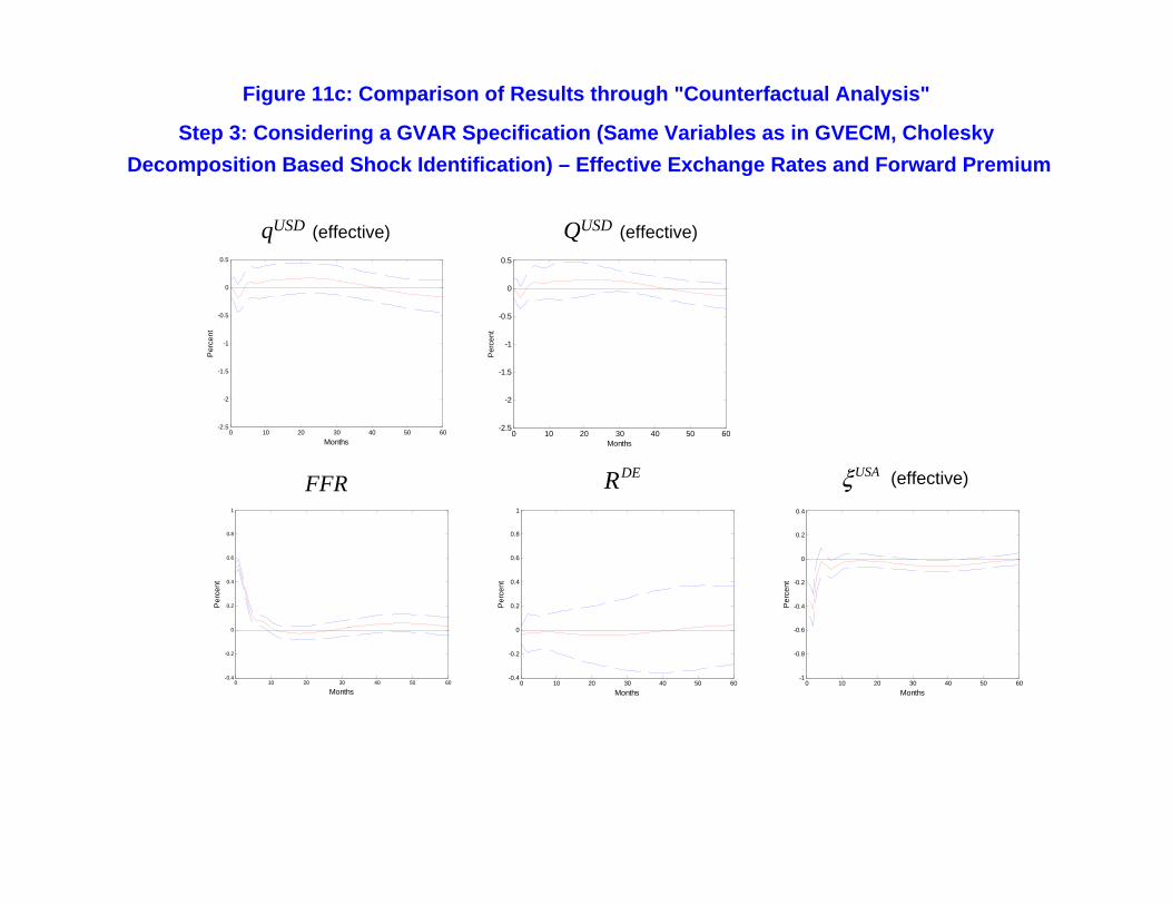
The third step of our counterfactual analysis is to move from the bilateral (two country) VAR set-

17

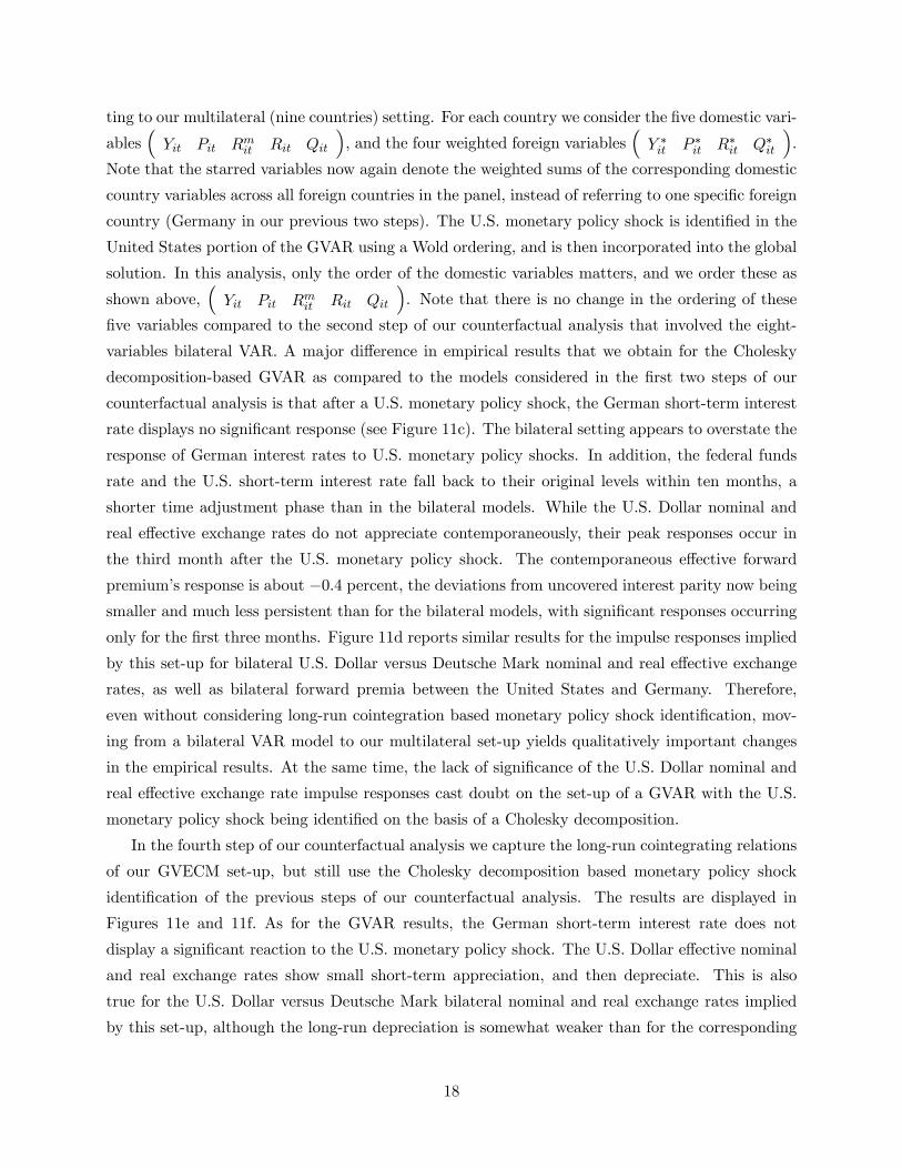
ting to our multilateral (nine countries) setting. For each country we consider the five domestic vari-

ables³Yit Pit Rm

it Rit Qit

´, and the four weighted foreign variables

³Y ∗it P ∗it R∗it Q∗it

´.

Note that the starred variables now again denote the weighted sums of the corresponding domestic

country variables across all foreign countries in the panel, instead of referring to one specific foreign

country (Germany in our previous two steps). The U.S. monetary policy shock is identified in the

United States portion of the GVAR using a Wold ordering, and is then incorporated into the global

solution. In this analysis, only the order of the domestic variables matters, and we order these as

shown above,³Yit Pit Rm

it Rit Qit

´. Note that there is no change in the ordering of these

five variables compared to the second step of our counterfactual analysis that involved the eight-

variables bilateral VAR. A major difference in empirical results that we obtain for the Cholesky

decomposition-based GVAR as compared to the models considered in the first two steps of our

counterfactual analysis is that after a U.S. monetary policy shock, the German short-term interest

rate displays no significant response (see Figure 11c). The bilateral setting appears to overstate the

response of German interest rates to U.S. monetary policy shocks. In addition, the federal funds

rate and the U.S. short-term interest rate fall back to their original levels within ten months, a

shorter time adjustment phase than in the bilateral models. While the U.S. Dollar nominal and

real effective exchange rates do not appreciate contemporaneously, their peak responses occur in

the third month after the U.S. monetary policy shock. The contemporaneous effective forward

premium’s response is about −0.4 percent, the deviations from uncovered interest parity now beingsmaller and much less persistent than for the bilateral models, with significant responses occurring

only for the first three months. Figure 11d reports similar results for the impulse responses implied

by this set-up for bilateral U.S. Dollar versus Deutsche Mark nominal and real effective exchange

rates, as well as bilateral forward premia between the United States and Germany. Therefore,

even without considering long-run cointegration based monetary policy shock identification, mov-

ing from a bilateral VAR model to our multilateral set-up yields qualitatively important changes

in the empirical results. At the same time, the lack of significance of the U.S. Dollar nominal and

real effective exchange rate impulse responses cast doubt on the set-up of a GVAR with the U.S.

monetary policy shock being identified on the basis of a Cholesky decomposition.

In the fourth step of our counterfactual analysis we capture the long-run cointegrating relations

of our GVECM set-up, but still use the Cholesky decomposition based monetary policy shock

identification of the previous steps of our counterfactual analysis. The results are displayed in

Figures 11e and 11f. As for the GVAR results, the German short-term interest rate does not

display a significant reaction to the U.S. monetary policy shock. The U.S. Dollar effective nominal

and real exchange rates show small short-term appreciation, and then depreciate. This is also

true for the U.S. Dollar versus Deutsche Mark bilateral nominal and real exchange rates implied

by this set-up, although the long-run depreciation is somewhat weaker than for the corresponding

18

effective U.S. Dollar exchange rates. The forward premium impulse responses, both measured as

effective forward premia for the United States and as bilateral forward premia for the United States

relative to Germany, are similar as in the level GVAR without long-run cointegrating relations as

was considered in the third step of our counterfactual analysis. The rather implausible nominal and

real long-run depreciation of the U.S. Dollar in response to a contractionary U.S. monetary policy

shock obtained in the GVECM setting of this step suggests that the Cholesky decomposition based

shock identification is rather problematic when applied to a model containing long-run restrictions.

For the fifth step of our counterfactual analysis we then move to our GVECM set-up with iden-

tifying restrictions similar to those in Section 4, namely cointegration- based long-run restrictions

augmented by as few short-run identifying restrictions as necessary, but now - unlike in Section 4 -

impose orthogonality of monetary policy shocks in all countries other than the United States. As

Figures 11g to 11j show, this helps tightening the impulse response standard error bands for the

German short-term interest rate, but for the impulse responses for the nominal and real effective

U.S. Dollar as well as bilateral U.S. Dollar versus Deutsche Mark exchange rates yields very similar

results as we had obtained in Section 4. (The impulse responses in Figures 11i and 11j are ob-

tained using our methodology of Section 4, except that they are plotted for a U.S. contractionary

monetary policy shock of 50 basis points, as in the previous steps of the counterfactual analysis

in this section.) Also, the impulse responses for the effective U.S. as well as bilateral U.S. versus

German forward premia are very similar to those we had obtained in Section 4. This suggests that

our assumptions in Section 4 regarding the presence of cross-country correlation of shocks abroad

with U.S. monetary policy shocks are not a driving force of our results.

Overall, the findings of our counterfactual analysis strongly suggest that both (i) our accounting

for multilateral (rather than just bilateral) cross-country adjustment in response to monetary policy

shocks, and (ii) our taking advantage of the identifying restrictions for monetary policy shocks

implied by long-run relations between the macroeconomic variables under consideration, are of

critical relevance in us being able to provide evidence that there is neither a delayed exchange rate

overshooting puzzle nor a forward premium puzzle in the adjustment of U.S. Dollar nominal and

real exchange rates and forward premia in response to U.S. monetary policy shocks.

6 Conclusion

In this paper we have re-considered the effects of monetary policy shocks on exchange rates and

forward premia. In the recent empirical literature these effects have been described as puzzling, in

that they would include delayed overshooting of the exchange rate as well as persistent deviations

from uncovered interest parity. We have constructed an empirical model that in particular (i) allows

for simultaneous multi-country adjustments in response to monetary policy shocks, and (ii) takes

19

advantage of the identifying restrictions for monetary policy shocks implied by long-run relations

between the macroeconomic variables under consideration. Using monthly data from 1978 to 2006

for a panel of nine industrial economies (Australia, Canada, France, Germany, Italy, Japan, New

Zealand, United Kingdom, and the United States), we have found that U.S. Dollar effective and

bilateral real exchange rates appreciate immediately after a contractionary U.S. monetary policy

shock, and that there is no delay in the overshooting of the U.S. Dollar. Furthermore, there is

no persistent significant forward premium and the price puzzle is at most weakly present. These

results suggest that existing open economy dynamic stochastic general equilibrium models inter

alia featuring staggered price setting actually are consistent with the data with regards to their

implications for the real exchange rate effects of monetary policy shocks.

20

References

[1] Armour, J., W. Engert, and B.S.C. Fung (1996): Overnight Rate Innovations as a Measure of Monetary

Policy Shocks in Vector Autoregressions, Working Paper, Bank of Canada.

[2] Bernanke, B.S., and A.S. Blinder (1992): The Federal Funds Rate and the Channels of Monetary

Transmission, American Economic Review, 82, pp. 901-921.

[3] Bernanke, B.S., and I. Mihov (1997): What Does The Bundesbank Target?, European Economic Review,

41, pp. 1025-1053.

[4] Bernanke, B.S., and I. Mihov (1998): Measuring Monetary Policy, Quarterly Journal of Economics,

113, pp. 869-902.

[5] Benigno, G. (2004): Real Exchange Rate Persistence and Monetary Policy Rules, Journal of Monetary

Economics, 51, pp. 473-502.

[6] Bjornland, H.C. (2006): Monetary Policy and Exchange Rate Overshooting: Dornbusch Was Right

After All, Scandinavian Journal of Economics (Forthcoming).

[7] Borio, C.V.E. (2001): Monetary Policy Operating Procedures in Industrial Countries, Working Paper,

Bank for International Settlements.

[8] Brueggemann, I. (2003): Measuring Monetary Policy in Germany: A Structural Vector Error Correction

Approach, German Economic Review, 4, pp. 307-339.

[9] Croushore, D., and C.L. Evans (2006): Data Revisions and the Identification of Monetary Policy Shocks,

Journal of Monetary Economics, 53, pp. 1135-1160,

[10] Cushman, D. O., and T. Zha (1997): Identifying Monetary Policy in a Small Open Economy under

Flexible Exchange Rates, Journal of Monetary Economics, 39, pp. 433-448.

[11] Dees, S., F. di Mauro, M.H. Pesaran, and L.V. Smith (2007): Exploring the International Linkages of

the Euro Area: A Global VAR Analysis, Journal of Applied Econometrics, 22, pp. 1-38.

[12] Eichenbaum, M., and C. Evans (1995): Some Empirical Evidence on the Effect of Monetary Policy

Shocks on Exchange Rates, Quarterly Journal of Economics, 110, pp. 975-1009.

[13] Faust, J., and J.H. Rogers (2003): Monetary Policy’s Role in Exchange Rate Behavior, Journal of

Monetary Economics, 50, pp. 1403-1424.

[14] Giordani, P. (2004): An Alternative Explanation of the Price Puzzle, Journal of Monetary Economics,

51, pp. 1271-1296.

[15] Kilian, L. (1998): Small-Sample Confidence Intervals for Impulse Response Functions, Review of Eco-

nomics and Statistics, 80, 218-230.

[16] Kim, S., and N. Roubini (2000): Exchange Rate Anomalies in the Industrial Countries: A Solution

with a Structural VAR Approach, Journal of Monetary Economics, 45, pp. 561-586.

[17] Luetkepohl, H. (2007): New Introduction to Multiple Time Series Analysis, Springer Verlag.

R1

[18] McCallum, B.T. (2003): Japanese Monetary Policy, Federal Reserve Bank of Richmond Economic Quar-

terly, 89, pp. 1-31.

[19] Miyao, R. (2001): The Effects of Monetary Policy in Japan, Journal of Money, Credit and Banking, 34,

pp. 376-392.

[20] Okina, K. (1993): Market Operations in Japan: Theory and Evidence, in J. Singleton (Ed.): Japanese

Monetary Policy, University of Chicago Press, pp. 31-62.

[21] Pagan, A.R., and M.H. Pesaran (2008): Econometric Analysis of Structural Systems with Permanent

and Transitory Shocks, Journal of Economic Dynamics and Control, 32, pp. 3376-3395.

[22] Peersmann, G. (2004): The Transmission of the Monetary Policy in the Euro Area: Are the Effects

Different Across Countries?, Oxford Bulletin of Economics and Statistics, 66, pp. 285-308.

[23] Peersman, G., and F. Smets (2001): The Monetary Transmission Mechanism in the Euro Area: More

Evidence from VAR Analysis, Working Paper, European Central Bank.

[24] Pesaran, M.H., T. Schuermann, and S.M. Weiner (2004): Modelling Regional Interdependencies Using

a Global Error Correcting Macroeconometric Model, Journal of Business and Economic Statistics, 22,

pp. 129-162.

[25] Pesaran, M.H., Y. Shin, and R.J. Smith (2000): Structural Analysis of Vector Error Correction Models

with Exogenous I(1) Variables, Journal of Econometrics, 97, pp. 293-343.

[26] Scholl, A., and H. Uhlig (2007): New Evidence on the Puzzles: Results from Agnostic Identification on

Monetary Policy and Exchange Rates, Working Paper, Humboldt University Berlin.

[27] Steinsson, J. (2008): The Dynamic Behavior of the Real Exchange Rate in Sticky Price Models, Amer-

ican Economic Review, 98, pp. 519-553.

[28] Strongin, S. (1995): The Identification of Monetary Policy Disturbances Explaining the Liquidity Puzzle,

Journal of Monetary Economics, 35, pp. 463-497.

R2

1

"Delayed Exchange Rate Overshooting

Puzzle"

"Forward Premium Puzzle"

Typical Finding Typical Finding in Empirical in Empirical LiteratureLiterature

Sticky Price Sticky Price Monetary ModelMonetary Model Typical Finding Typical Finding

in Empirical in Empirical LiteratureLiterature

Sticky Price Sticky Price Monetary ModelMonetary Model

Figure 1: The Delayed Exchange Rate Overshooting and Forward Premium Puzzles

/ /USD ForeignCurrency USD ForeignCurrencyt t

ForeignCountry USAt t

q QP P

=

+ −

/

/ /1( )

USA ForeignCountry USA ForeignCountryt t t

USD ForeignCurrency USD ForeignCurrencyt t

R RQ Q+

= − +

+ −

ξ

Figure 2: Key Results of Eichenbaum and Evans (1995)

qUSD/DM

DER /USD DEξ

FFR

0 10 20 30 40 50 60-1

-0.8

-0.6

-0.4

-0.2

0

0.2

0.4

Months

Per

cent

0 10 20 30 40 50 60-2.5

-2

-1.5

-1

-0.5

0

0.5

Months

Per

cent

0 10 20 30 40 50 60-0.4

-0.2

0

0.2

0.4

0.6

0.8

1

Months

Per

cent

0 10 20 30 40 50 60-0.4

-0.2

0

0.2

0.4

0.6

0.8

1

Months

Per

cent

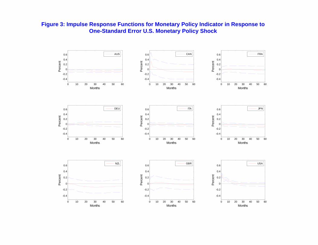
Figure 3: Impulse Response Functions for Monetary Policy Indicator in Response to One-Standard Error U.S. Monetary Policy Shock

0 10 20 30 40 50 60

-0.4

-0.2

0

0.2

0.4

0.6

Months

Per

cent

AUS

0 10 20 30 40 50 60

-0.4

-0.2

0

0.2

0.4

0.6

Months

Per

cent

CAN

0 10 20 30 40 50 60

-0.4

-0.2

0

0.2

0.4

0.6

Months

Per

cent

FRA

0 10 20 30 40 50 60

-0.4

-0.2

0

0.2

0.4

0.6

Months

Per

cent

DEU

0 10 20 30 40 50 60

-0.4

-0.2

0

0.2

0.4

0.6

MonthsP

erce

nt

ITA

0 10 20 30 40 50 60

-0.4

-0.2

0

0.2

0.4

0.6

Months

Per

cent

JPN

0 10 20 30 40 50 60

-0.4

-0.2

0

0.2

0.4

0.6

Months

Per

cent

NZL

0 10 20 30 40 50 60

-0.4

-0.2

0

0.2

0.4

0.6

Months

Per

cent

GBR

0 10 20 30 40 50 60

-0.4

-0.2

0

0.2

0.4

0.6

Months

Per

cent

USA

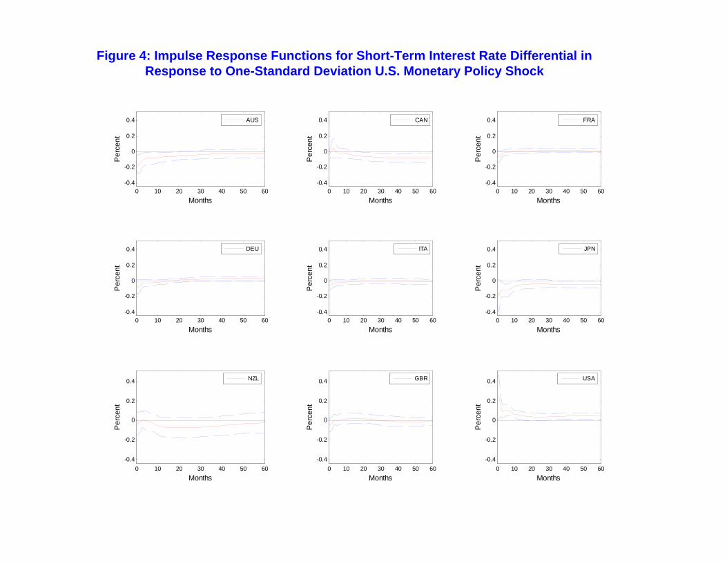
Figure 4: Impulse Response Functions for Short-Term Interest Rate Differential in Response to One-Standard Deviation U.S. Monetary Policy Shock

0 10 20 30 40 50 60-0.4

-0.2

0

0.2

0.4

Months

Per

cent

AUS

0 10 20 30 40 50 60-0.4

-0.2

0

0.2

0.4

Months

Per

cent

CAN

0 10 20 30 40 50 60-0.4

-0.2

0

0.2

0.4

Months

Per

cent

FRA

0 10 20 30 40 50 60-0.4

-0.2

0

0.2

0.4

Months

Per

cent

DEU

0 10 20 30 40 50 60-0.4

-0.2

0

0.2

0.4

Months

Per

cent

ITA

0 10 20 30 40 50 60-0.4

-0.2

0

0.2

0.4

Months

Per

cent

JPN

0 10 20 30 40 50 60-0.4

-0.2

0

0.2

0.4

Months

Per

cent

NZL

0 10 20 30 40 50 60-0.4

-0.2

0

0.2

0.4

Months

Per

cent

GBR

0 10 20 30 40 50 60-0.4

-0.2

0

0.2

0.4

MonthsP

erce

nt

USA

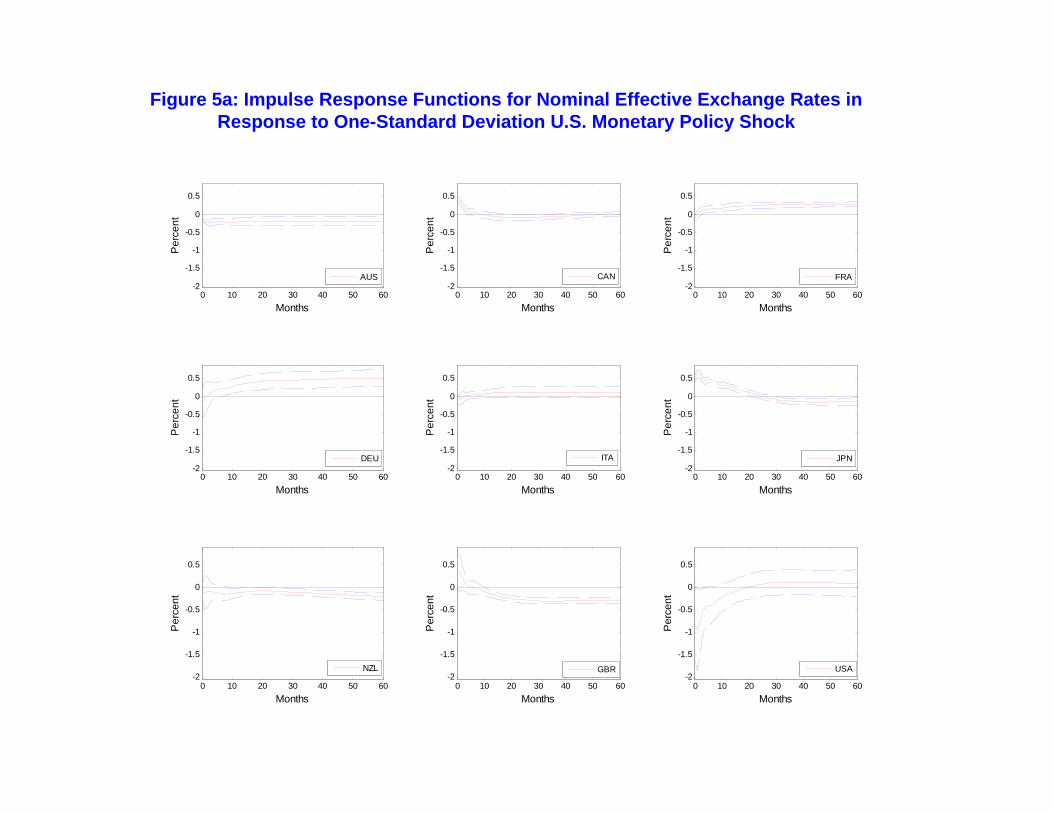
Figure 5a: Impulse Response Functions for Nominal Effective Exchange Rates in Response to One-Standard Deviation U.S. Monetary Policy Shock

0 10 20 30 40 50 60-2

-1.5

-1

-0.5

0

0.5

Months

Per

cent

AUS

0 10 20 30 40 50 60-2

-1.5

-1

-0.5

0

0.5

Months

Per

cent

CAN

0 10 20 30 40 50 60-2

-1.5

-1

-0.5

0

0.5

Months

Per

cent

FRA

0 10 20 30 40 50 60-2

-1.5

-1

-0.5

0

0.5

Months

Per

cent

DEU

0 10 20 30 40 50 60-2

-1.5

-1

-0.5

0

0.5

Months

Per

cent

ITA

0 10 20 30 40 50 60-2

-1.5

-1

-0.5

0

0.5

Months

Per

cent

JPN

0 10 20 30 40 50 60-2

-1.5

-1

-0.5

0

0.5

Months

Per

cent

NZL

0 10 20 30 40 50 60-2

-1.5

-1

-0.5

0

0.5

Months

Per

cent

GBR

0 10 20 30 40 50 60-2

-1.5

-1

-0.5

0

0.5

Months

Per

cent

USA

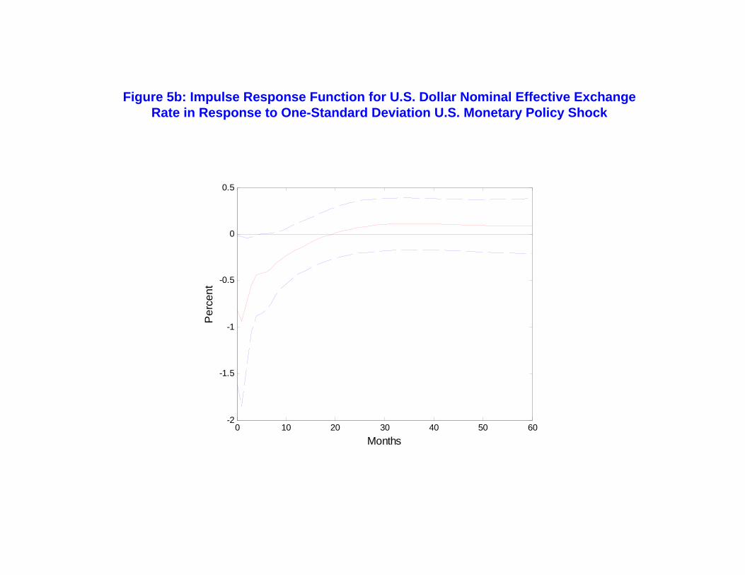
Figure 5b: Impulse Response Function for U.S. Dollar Nominal Effective Exchange Rate in Response to One-Standard Deviation U.S. Monetary Policy Shock

0 10 20 30 40 50 60-2

-1.5

-1

-0.5

0

0.5

Months

Per

cent

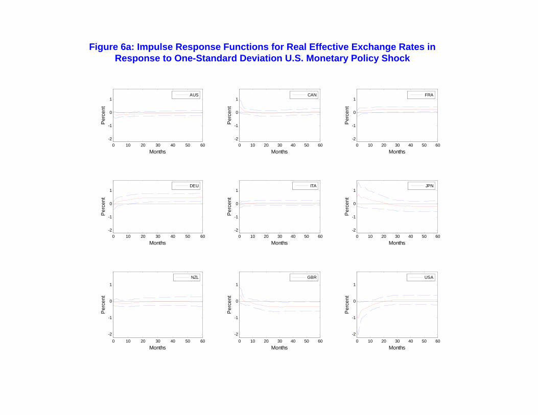
Figure 6a: Impulse Response Functions for Real Effective Exchange Rates in Response to One-Standard Deviation U.S. Monetary Policy Shock

0 10 20 30 40 50 60-2

-1

0

1

Months

Per

cent

0 10 20 30 40 50 60-2

-1

0

1

Months

Per

cent

0 10 20 30 40 50 60-2

-1

0

1

Months

Per

cent

0 10 20 30 40 50 60-2

-1

0

1

Months

Per

cent

0 10 20 30 40 50 60-2

-1

0

1

Months

Per

cent

0 10 20 30 40 50 60-2

-1

0

1

Months

Per

cent

0 10 20 30 40 50 60-2

-1

0

1

Months

Per

cent

0 10 20 30 40 50 60-2

-1

0

1

Months

Per

cent

0 10 20 30 40 50 60-2

-1

0

1

MonthsP

erce

nt

USAGBRNZL

JPNITADEU

FRACANAUS

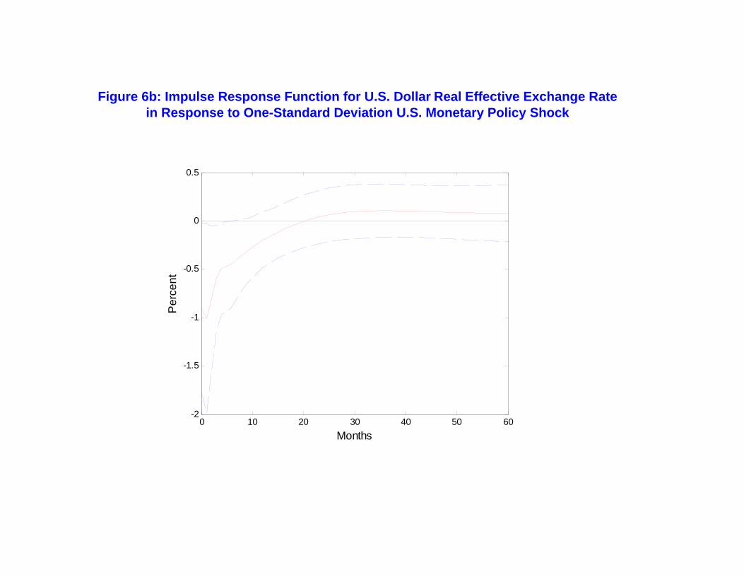
Figure 6b: Impulse Response Function for U.S. Dollar Real Effective Exchange Rate in Response to One-Standard Deviation U.S. Monetary Policy Shock

0 10 20 30 40 50 60-2

-1.5

-1

-0.5

0

0.5

Months

Per

cent

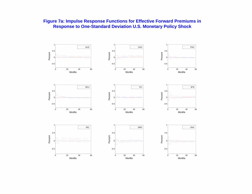
Figure 7a: Impulse Response Functions for Effective Forward Premiums in Response to One-Standard Deviation U.S. Monetary Policy Shock

0 20 40 60

-0.5

0

0.5

1

Months

Per

cent

0 20 40 60

-0.5

0

0.5

1

Months

Per

cent

0 20 40 60

-0.5

0

0.5

1

Months

Per

cent

0 20 40 60

-0.5

0

0.5

1

Months

Per

cent

0 20 40 60

-0.5

0

0.5

1

MonthsP

erce

nt0 20 40 60

-0.5

0

0.5

1

Months

Per

cent

0 20 40 60

-0.5

0

0.5

1

Months

Per

cent

0 20 40 60

-0.5

0

0.5

1

Months

Per

cent

0 20 40 60

-0.5

0

0.5

1

MonthsP

erce

nt

AUS CAN FRA

DEU ITA JPN

NZL GBR USA

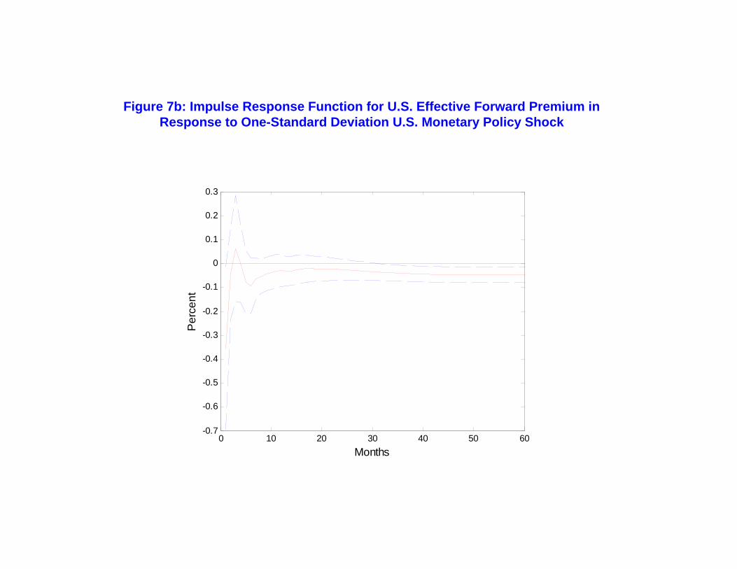
Figure 7b: Impulse Response Function for U.S. Effective Forward Premium in Response to One-Standard Deviation U.S. Monetary Policy Shock

0 10 20 30 40 50 60-0.7

-0.6

-0.5

-0.4

-0.3

-0.2

-0.1

0

0.1

0.2

0.3

Months

Per

cent

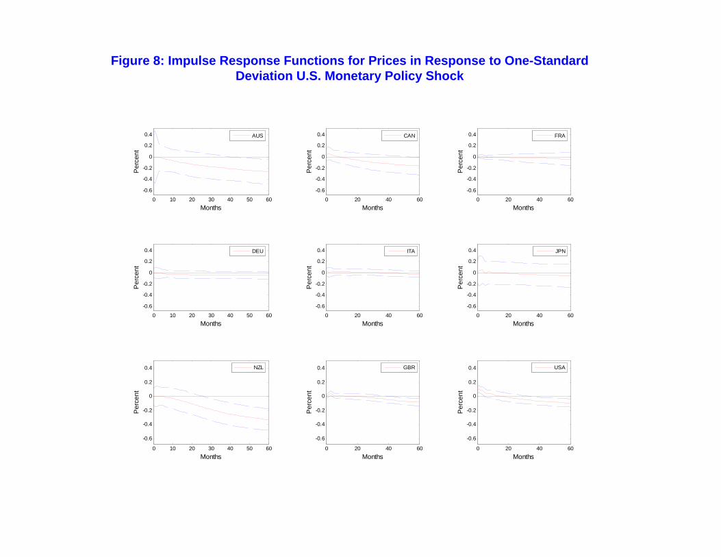
Figure 8: Impulse Response Functions for Prices in Response to One-Standard Deviation U.S. Monetary Policy Shock

0 10 20 30 40 50 60

-0.6

-0.4

-0.2

0

0.2

0.4

Months

Per

cent

0 20 40 60

-0.6

-0.4

-0.2

0

0.2

0.4

Months

Per

cent

0 20 40 60

-0.6

-0.4

-0.2

0

0.2

0.4

Months

Per

cent

0 10 20 30 40 50 60

-0.6

-0.4

-0.2

0

0.2

0.4

Months

Per

cent

0 20 40 60

-0.6

-0.4

-0.2

0

0.2

0.4

Months

Per

cent

0 20 40 60

-0.6

-0.4

-0.2

0

0.2

0.4

Months

Per

cent

0 10 20 30 40 50 60

-0.6

-0.4

-0.2

0

0.2

0.4

Months

Per

cent

0 20 40 60

-0.6

-0.4

-0.2

0

0.2

0.4

Months

Per

cent

0 20 40 60

-0.6

-0.4

-0.2

0

0.2

0.4

MonthsP

erce

nt

AUS CAN FRA

DEU ITA JPN

NZL GBR USA

Eichen-baum and

Evans (1995)

GVECM

Sticky Price Monetary

Model

Figure 9: Comparison of Some Key Results

qUSD/ForeignCurrency /USA ForeignCountryξUSA ForeignCountryR R−

qUSD (effective) USAR DER

qUSD/DM FFR DER/USA DEξ

USAξ (effective)

0 10 20 30 40 50 60-1

-0.8

-0.6

-0.4

-0.2

0

0.2

0.4

Months

Per

cent

0 10 20 30 40 50 60-2.5

-2

-1.5

-1

-0.5

0

0.5

Months

Per

cent

0 10 20 30 40 50 60-0.4

-0.2

0

0.2

0.4

0.6

0.8

1

Months

Per

cent

0 10 20 30 40 50 60-0.4

-0.2

0

0.2

0.4

0.6

0.8

1

Months

Per

cent

0 10 20 30 40 50 60-2.5

-2

-1.5

-1

-0.5

0

0.5

Months

Per

cent

0 10 20 30 40 50 60-0.4

-0.2

0

0.2

0.4

0.6

0.8

1

Months

Per

cent

0 10 20 30 40 50 60-0.4

-0.2

0

0.2

0.4

0.6

0.8

1

Months

Per

cent

0 10 20 30 40 50 60-1

-0.8

-0.6

-0.4

-0.2

0

0.2

0.4

Months

Per

cent

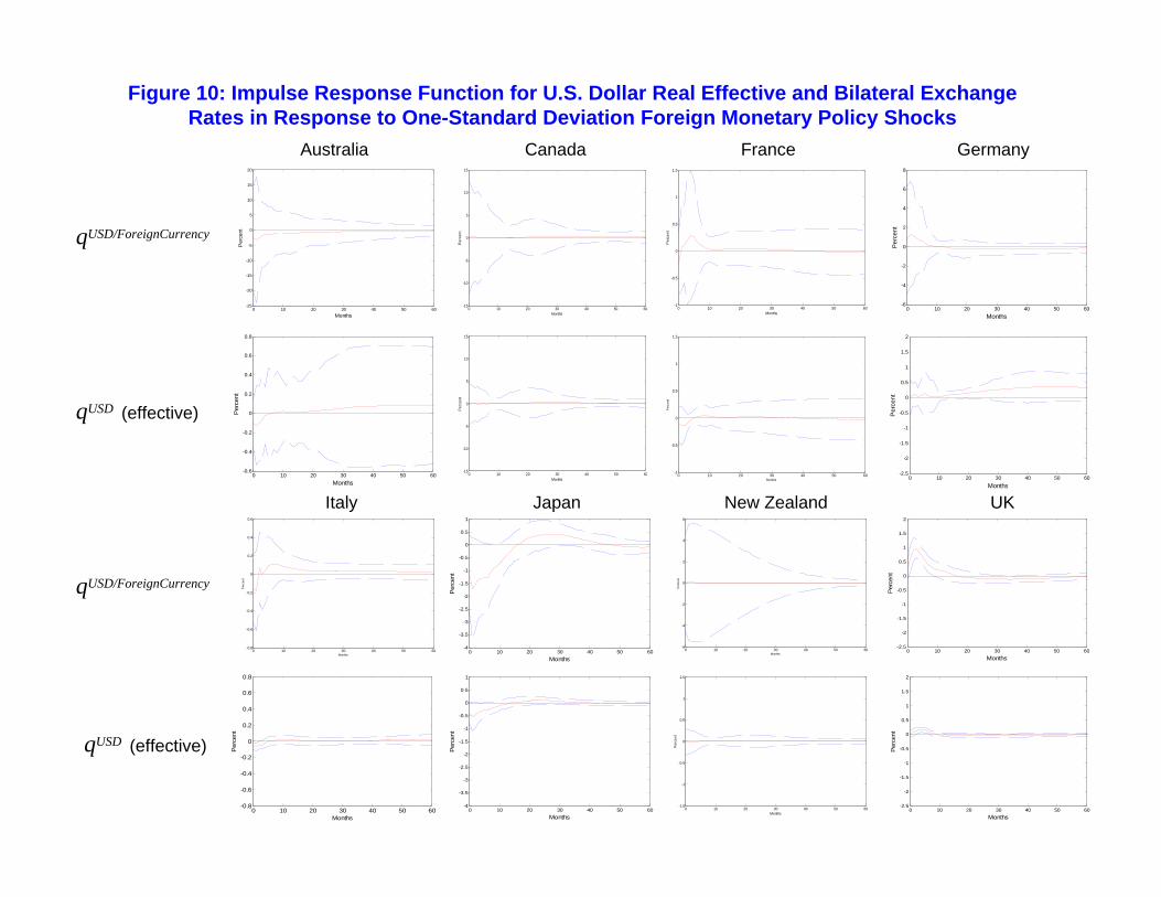
Figure 10: Impulse Response Function for U.S. Dollar Real Effective and Bilateral Exchange Rates in Response to One-Standard Deviation Foreign Monetary Policy Shocks

0 10 20 30 40 50 60-0.6

-0.4

-0.2

0

0.2

0.4

0.6

0.8

Months

Per

cent

0 10 20 30 40 50 60-25

-20

-15

-10

-5

0

5

10

15

20

Months

Per

cent

Australia

0 10 20 30 40 50 60-15

-10

-5

0

5

10

15

Months

Per

cent

0 10 20 30 40 50 60-15

-10

-5

0

5

10

15

Months

Per

cent

Canada

0 10 20 30 40 50 60-1

-0.5

0

0.5

1

1.5

Months

Per

cent

0 10 20 30 40 50 60-1

-0.5

0

0.5

1

1.5

Months

Per

cent

France

0 10 20 30 40 50 60-6

-4

-2

0

2

4

6

8

Months

Per

cent

0 10 20 30 40 50 60-2.5

-2

-1.5

-1

-0.5

0

0.5

1

1.5

2

Months

Per

cent

Germany

0 10 20 30 40 50 60-0.8

-0.6

-0.4

-0.2

0

0.2

0.4

0.6

Months

Per

cent

0 10 20 30 40 50 60-0.8

-0.6

-0.4

-0.2

0

0.2

0.4

0.6

0.8

Months

Per

cent

Italy

0 10 20 30 40 50 60-4

-3.5

-3

-2.5

-2

-1.5

-1

-0.5

0

0.5

1

Months

Per

cent

0 10 20 30 40 50 60-4

-3.5

-3

-2.5

-2

-1.5

-1

-0.5

0

0.5

1

Months

Per

cent

Japan

0 10 20 30 40 50 60-6

-4

-2

0

2

4

6

Months

Per

cent

0 10 20 30 40 50 60-1.5

-1

-0.5

0

0.5

1

1.5

Months

Per

cent

New Zealand

0 10 20 30 40 50 60-2.5

-2

-1.5

-1

-0.5

0

0.5

1

1.5

2

Months

Per

cent

0 10 20 30 40 50 60-2.5

-2

-1.5

-1

-0.5

0

0.5

1

1.5

2

Months

Per

cent

qUSD/ForeignCurrency

qUSD (effective)

qUSD (effective)

qUSD/ForeignCurrency

UK

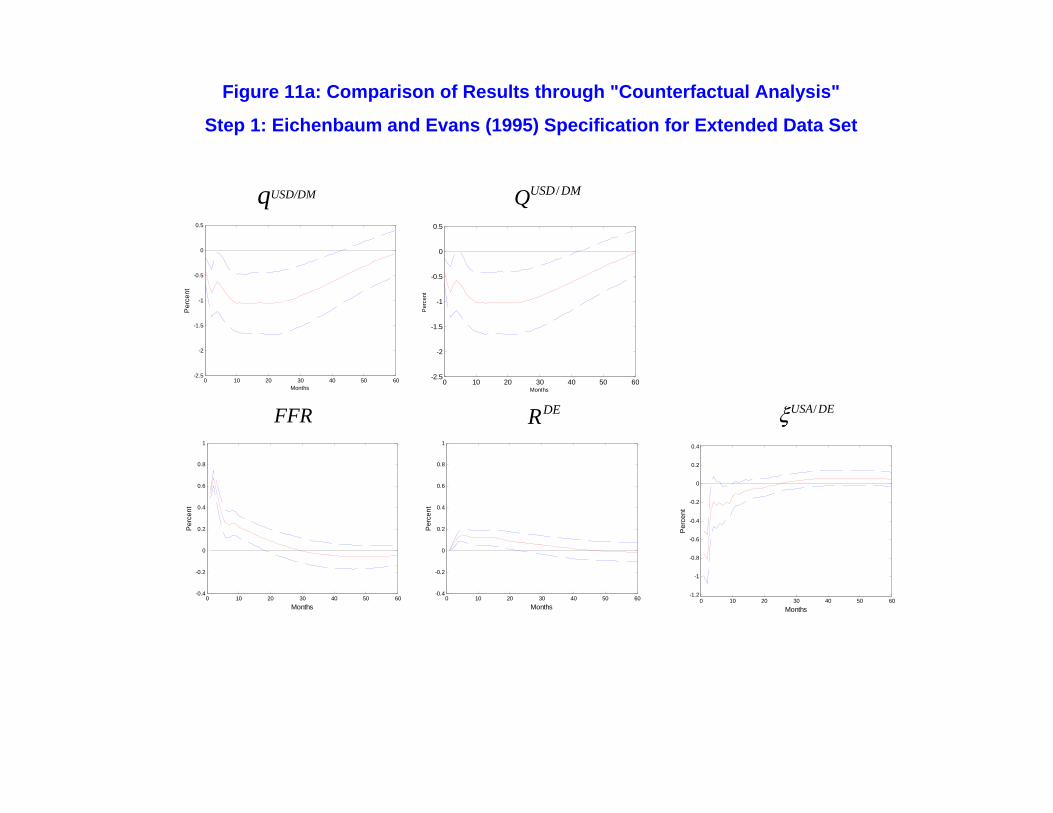
Figure 11a: Comparison of Results through "Counterfactual Analysis"

Step 1: Eichenbaum and Evans (1995) Specification for Extended Data Set

qUSD/DM /USD DMQ

FFR /USA DEξDER

0 10 20 30 40 50 60-2.5

-2

-1.5

-1

-0.5

0

0.5

Months

Per

cent

0 10 20 30 40 50 60-2.5

-2

-1.5

-1

-0.5

0

0.5

Months

Per

cent

0 10 20 30 40 50 60-0.4

-0.2

0

0.2

0.4

0.6

0.8

1

Months

Per

cent

0 10 20 30 40 50 60-0.4

-0.2

0

0.2

0.4

0.6

0.8

1

Months

Per

cent

0 10 20 30 40 50 60-1.2

-1

-0.8

-0.6

-0.4

-0.2

0

0.2

0.4

Months

Per

cent

qUSD/DM /USD DMQ

FFR

Figure 11b: Comparison of Results through "Counterfactual Analysis"

Step 2: Augmenting Eichenbaum and Evans (1995) Specification to Capture Same Variables asEntering GVECM

DER/USA DEξ

0 10 20 30 40 50 60-2.5

-2

-1.5

-1

-0.5

0

0.5

Months

Per

cent

0 10 20 30 40 50 60-2.5

-2

-1.5

-1

-0.5

0

0.5

Months

Per

cent

0 10 20 30 40 50 60-0.4

-0.2

0

0.2

0.4

0.6

0.8

1

Months

Per

cent

0 10 20 30 40 50 60-0.4

-0.2

0

0.2

0.4

0.6

0.8

1

Months

Per

cent

0 10 20 30 40 50 60-1

-0.8

-0.6

-0.4

-0.2

0

0.2

0.4

Months

Per

cent

FFR

Figure 11c: Comparison of Results through "Counterfactual Analysis"

Step 3: Considering a GVAR Specification (Same Variables as in GVECM, CholeskyDecomposition Based Shock Identification) – Effective Exchange Rates and Forward Premium

qUSD (effective) QUSD (effective)

DER (effective)USAξ

0 10 20 30 40 50 60-2.5

-2

-1.5

-1

-0.5

0

0.5

Months

Per

cent

0 10 20 30 40 50 60-2.5

-2

-1.5

-1

-0.5

0

0.5

Months

Per

cent

0 10 20 30 40 50 60-0.4

-0.2

0

0.2

0.4

0.6

0.8

1

Months

Per

cent

0 10 20 30 40 50 60-0.4

-0.2

0

0.2

0.4

0.6

0.8

1

Months

Per

cent

0 10 20 30 40 50 60-1

-0.8

-0.6

-0.4

-0.2

0

0.2

0.4

Months

Per

cent

qUSD/DM /USD DMQ

FFR

Figure 11d: Comparison of Results through "Counterfactual Analysis"

Step 3: Considering a GVAR Specification (Same Variables as in GVECM, CholeskyDecomposition Based Shock Identification) – Bilateral Exchange Rates and Forward Premium

DER /USA DEξ

0 10 20 30 40 50 60-2.5

-2

-1.5

-1

-0.5

0

0.5

Months

Per

cent

0 10 20 30 40 50 60-2.5

-2

-1.5

-1

-0.5

0

0.5

Months

Per

cent

0 10 20 30 40 50 60-0.4

-0.2

0

0.2

0.4

0.6

0.8

1

Months

Per

cent

0 10 20 30 40 50 60-0.4

-0.2

0

0.2

0.4

0.6

0.8

1

Months

Per

cent

0 10 20 30 40 50 60-1

-0.8

-0.6

-0.4

-0.2

0

0.2

0.4

Months

Per

cent

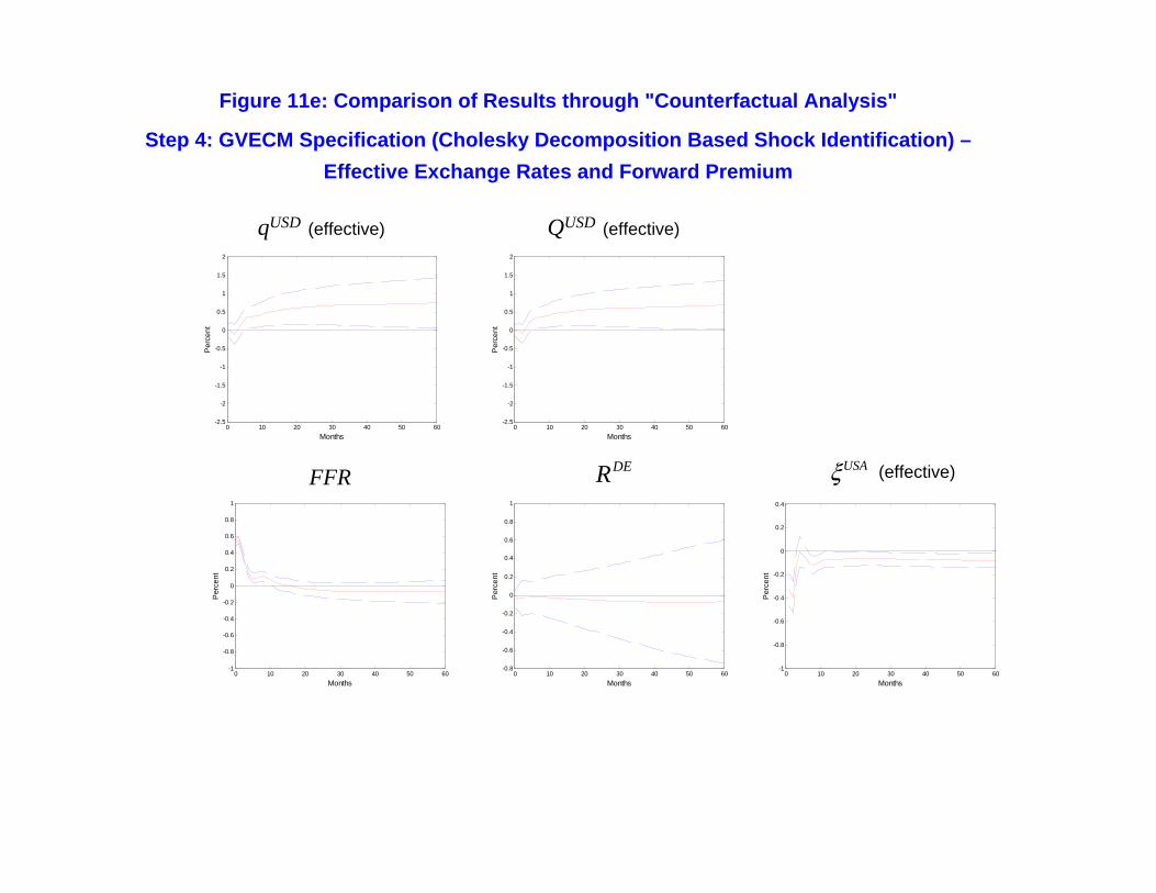
FFR

qUSD (effective) QUSD (effective)

DER (effective)USAξ

Figure 11e: Comparison of Results through "Counterfactual Analysis"

Step 4: GVECM Specification (Cholesky Decomposition Based Shock Identification) –Effective Exchange Rates and Forward Premium

0 10 20 30 40 50 60-2.5

-2

-1.5

-1

-0.5

0

0.5

1

1.5

2

Months

Per

cent

0 10 20 30 40 50 60-2.5

-2

-1.5

-1

-0.5

0

0.5

1

1.5

2

Months

Per

cent

0 10 20 30 40 50 60-1

-0.8

-0.6

-0.4

-0.2

0

0.2

0.4

0.6

0.8

1

Months

Per

cent

0 10 20 30 40 50 60-0.8

-0.6

-0.4

-0.2

0

0.2

0.4

0.6

0.8

1

Months

Per

cent

0 10 20 30 40 50 60-1

-0.8

-0.6

-0.4

-0.2

0

0.2

0.4

Months

Per

cent

qUSD/DM

FFR DER /USA DEξ

Figure 11f: Comparison of Results through "Counterfactual Analysis"

Step 4: GVECM Specification (Cholesky Decomposition Based Shock Identification) –Bilateral Exchange Rates and Forward Premium

0 10 20 30 40 50 60-2.5

-2

-1.5

-1

-0.5

0

0.5

1

1.5

Months

Per

cent

0 10 20 30 40 50 60-2.5

-2

-1.5

-1

-0.5

0

0.5

1

Months

Per

cent

0 10 20 30 40 50 60-1

-0.8

-0.6

-0.4

-0.2

0

0.2

0.4

0.6

0.8

1

Months

Per

cent

0 10 20 30 40 50 60-0.8

-0.6

-0.4

-0.2

0

0.2

0.4

0.6

0.8

1

Months

Per

cent

0 10 20 30 40 50 60-1

-0.8

-0.6

-0.4

-0.2

0

0.2

0.4

0.6

0.8

Months

Per

cent

/USD DMQ

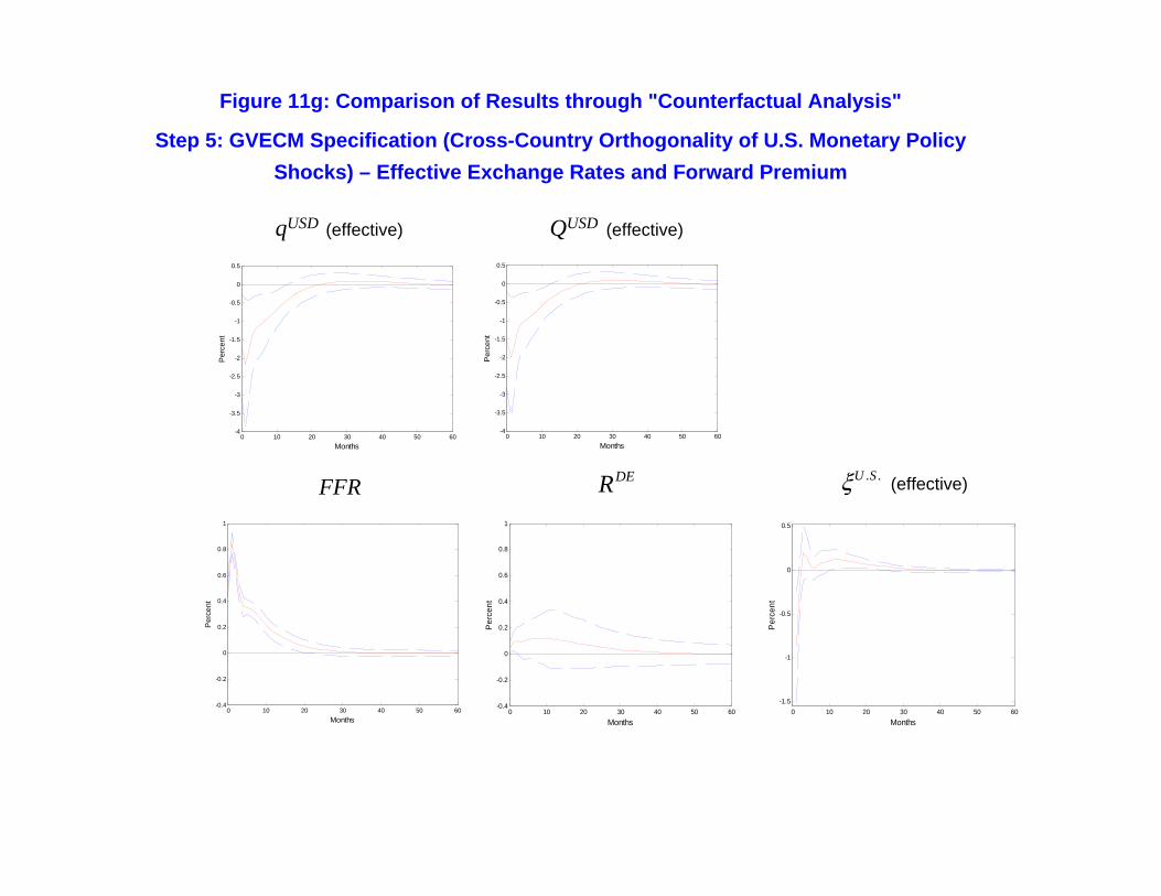
FFR

qUSD (effective) QUSD (effective)

DER (effective). .U Sξ

Figure 11g: Comparison of Results through "Counterfactual Analysis"

Step 5: GVECM Specification (Cross-Country Orthogonality of U.S. Monetary Policy Shocks) – Effective Exchange Rates and Forward Premium

0 10 20 30 40 50 60-4

-3.5

-3

-2.5

-2

-1.5

-1

-0.5

0

0.5

Months

Per

cent

0 10 20 30 40 50 60-4

-3.5

-3

-2.5

-2

-1.5

-1

-0.5

0

0.5

Months

Per

cent

0 10 20 30 40 50 60-0.4

-0.2

0

0.2

0.4

0.6

0.8

1

Months

Per

cent

0 10 20 30 40 50 60-0.4

-0.2

0

0.2

0.4

0.6

0.8

1

Months

Per

cent

0 10 20 30 40 50 60-1.5

-1

-0.5

0

0.5

Months

Per

cent

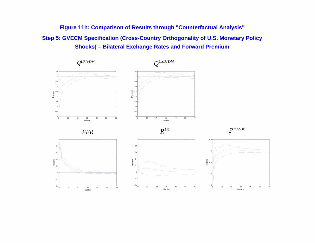
FFR DER

Figure 11h: Comparison of Results through "Counterfactual Analysis"

Step 5: GVECM Specification (Cross-Country Orthogonality of U.S. Monetary Policy Shocks) – Bilateral Exchange Rates and Forward Premium

qUSD/DM /USD DMQ

/USA DEξ

0 10 20 30 40 50 60-4

-3.5

-3

-2.5

-2

-1.5

-1

-0.5

0

0.5

Months

Per

cent

0 10 20 30 40 50 60-4

-3.5

-3

-2.5

-2

-1.5

-1

-0.5

0

0.5

Months

Per

cent

0 10 20 30 40 50 60-0.4

-0.2

0

0.2

0.4

0.6

0.8

1

Months

Per

cent

0 10 20 30 40 50 60-0.4

-0.2

0

0.2

0.4

0.6

0.8

1

Months

Per

cent

0 10 20 30 40 50 60-1.5

-1

-0.5

0

0.5

Months

Per

cent

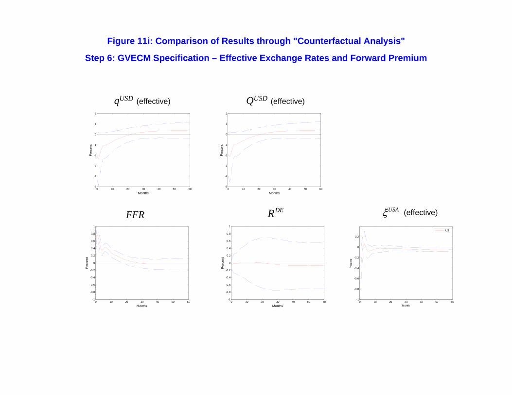
FFR

Figure 11i: Comparison of Results through "Counterfactual Analysis"

Step 6: GVECM Specification – Effective Exchange Rates and Forward Premium

qUSD (effective) QUSD (effective)

(effective)DER

0 10 20 30 40 50 60-1

-0.8

-0.6

-0.4

-0.2

0

0.2

Month

Per

cent

US

USAξ

0 10 20 30 40 50 60-5

-4

-3

-2

-1

0

1

2

Months

Per

cent

0 10 20 30 40 50 60-5

-4

-3

-2

-1

0

1

2

Months

Per

cent

0 10 20 30 40 50 60-1

-0.8

-0.6

-0.4

-0.2

0

0.2

0.4

0.6

0.8

1

Months

Per

cent

0 10 20 30 40 50 60-1

-0.8

-0.6

-0.4

-0.2

0

0.2

0.4

0.6

0.8

1

Months

Per

cent

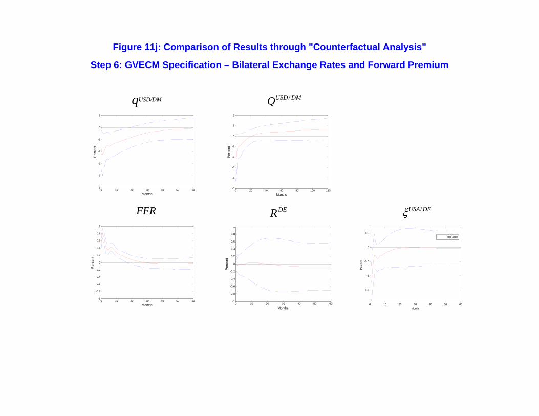
qUSD/DM /USD DMQ

FFR

Figure 11j: Comparison of Results through "Counterfactual Analysis"

Step 6: GVECM Specification – Bilateral Exchange Rates and Forward Premium

DER /USA DEξ

0 10 20 30 40 50 60-1

-0.8

-0.6

-0.4

-0.2

0

0.2

0.4

0.6

0.8

1

Months

Per

cent

0 10 20 30 40 50 60-1

-0.8

-0.6

-0.4

-0.2

0

0.2

0.4

0.6

0.8

1

Months

Per

cent

0 10 20 30 40 50 60-5

-4

-3

-2

-1

0

1

Months

Per

cent

0 20 40 60 80 100 120-5

-4

-3

-2

-1

0

1

2

Months

Per

cent

0 10 20 30 40 50 60

-1.5

-1

-0.5

0

0.5

Month

Per

cent

bfp-usde