NO. 0827S P D I S C U S S I O N P A P E R

On the Financial Sustainabilityof Earnings-Related PensionSchemes With “Pay-As-You-Go” Financing

David A. RobalinoAndrás Bodor

July 2008

On the Financial Sustainability of

Earnings-Related Pension Schemes

With “Pay-As-You-Go” Financing

David A. Robalino

András Bodor

July 2008

PENSION

REFORM

PRIMERrē-for´m

v.t. & i. 1. make (institution, procedure

etc.) better by removal or abandonment

of imperfections, faults or errors

prīmer n. 1. elementary book to

equip person with information

pe´nsion n.

1. perio

dic paym

ent

made esp. by g

overnment or em

ployer

on retirem

ent or to pers

on above

specified

age

On the Financial Sustainability of

Earnings-Related Pension Schemes

With “Pay-As-You-Go” Financing

David A. Robalino1

András Bodor2

The authors thank Robert Palacios, Edward Whitehouse, Michal Rutkowski, Alberto Musalem, and Robert Holzmann, for useful discussions and insights on the subject, and to Oleksiy Sluchinsky and Anca Mataoanu for commenting on early drafts. The current paper is based on a longer version published in the Journal of Pension Economics and Finance that also discusses the role of GDP indexed bonds as a mechanism to improve financial sustainability while making the implicit debt of the pay-as-you-go system explicit. The opinions presented in this paper do not necessarily represent the views of the World Bank or Georgetown University.

1 World Bank. 2 World Bank and Georgetown University

2

Abstract

In this paper we review the characterization of the sustainable rate of return of an earnings-related pension system with pay-as-you-go financing. We show that current proxies for the sustainable rate, including the Swedish “gyroscope”, are not stable and propose an alternative measure that depends on the growth of the buffer-stock and the pay-as-you-go asset. Using a simple one-sector macroeconomic model that embeds a notional account pension system we test how the different proxies perform in the presence of various macroeconomic and demographic shocks. We find that the new formula proposed in this paper is the most stable. It avoids the accumulation of assets without bound (which penalizes workers) while always ensuring a positive buffer fund. JEL Classification: H55, J14, J26 Keywords: earnings related pensions, financial sustainability, pay-as-you-go systems, public pensions

3

Table of contents

1. Introduction................................................................................................................. 4 2. The Sustainable Rate of Return of an ER System ...................................................... 6 3. Simulating the robustness of alternative rules for the IRR of the system................. 15 4. Discussions and Policy Implications ........................................................................ 27 References:.................................................................................................................... 28 Appendix 1 - Derivations.............................................................................................. 30 Appendix 2 - The Macro Model .................................................................................. 32 Appendix 3 – Sensitivity/Robustness Analysis ............................................................ 35

List of Figures

Figure 1: Financing Gap and the IRR................................................................................ 8 Figure 2: Dynamics of the Reserves/GDP Ratio When Annuity Does Not Include a Discount Rate.................................................................................................................... 20 Figure 3: Evolution of the Reserves/GDP Ratio when the Annuity Includes a Discount Rate ................................................................................................................................... 22 Figure 4: Dynamics of the Turnover Duration in the Swedish Stabilization System...... 26

List of Tables

Table 1: State for Key Model Variables .......................................................................... 17 Table 2: Descriptive Statistics for Selected Outputs........................................................ 23

4

1. INTRODUCTION

A majority of mandatory public pension systems in the world involve an earnings-

related (ER) scheme with “pay-as-you-go” financing. By earnings-related we refer to

systems where the pension is essentially a function of past earnings. Three main designs

can be identified: standard defined benefit systems, points systems, and notional account

systems; mathematically, the three benefit formulas are equivalent.3 By pay-as-you-go

we imply that pensions are financed essentially out of current contributions. Many of the

systems can have reserves, but these act rather as a “buffer stock” to smooth adjustments

to benefits or contribution rates that become necessary as a result of unexpected

macroeconomic and/or demographic shocks or the gradual maturation of the system.

Surprisingly, in most cases, ER systems do not meet basic principles in terms of

design to ensure financial sustainability, minimize distortions in labor supply and savings

decisions, and to avoid arbitrary -- often regressive -- redistributions of income. Even in

countries that have recently adopted notional account schemes, which deal with issues

related to incentives and equity, the problem of financial sustainability has not been fully

resolved.

The focus of this paper is on this last problem: the financial sustainability of the

scheme. It is well known that whether an ER system is financially self-sustainable or not

depends on the implicit rate of return (IRR) that it pays on contributions. If the IRR is

too high, the system becomes insolvent; if the IRR is too low the system penalizes

workers. Until recently, it was common to refer to the growth rate of the covered wage

bill as the appropriate measure of the IRR. This is the correct measure, however, only in

restrictive theoretical settings (e.g., two overlapping generation models in steady state).

Reality is more complex and while the growth rate of the covered wage bill can be a good

proxy under some circumstances, other factors such as retirement patterns, mortality

rates, and the age-sex composition of the plan members are important as well.

3 For discussions in terms of design and implementation of Notional Account systems see Holzmann and Palmer (2006), for the equivalence of benefit formulas see Cichon (1999), Devolder (2005) and Robalino et al. (2005).

5

Settergren and Mikula (2005) proposed a measure of the sustainable IRR that

inspires the “automatic balancing mechanism” in the current Swedish Notional Account

pension system. It depends on the growth rate of the average wage, the growth rate of

reserves, and the so called “turnover duration” (TD) of the system. The TD is supposed

to capture the average length of time that a monetary unit of contribution remains in the

system. The authors argue that the TD multiplied by total contributions at a given point

in time provides an estimate of the pension liability that can be supported by the system.

We argue, however, that this measure can be arbitrary and we show that it is not bullet

proof either; the system can deviate from long term equilibrium in the presence of shocks

to wages and coverage rates.4

Another approach has been recently proposed in Valdés-Prieto (2005a) and

applied to the case of the United States in Valdés-Prieto (2005b). The idea is to grant to

the pension fund property rights over the pay-as-you-go asset (the present value of future

contributions net of pension rights accruing from these contribution) through Covered

Wage Bill Bonds (CWB) – which are issued by the pension fund not the government.

Investors in the bonds basically acquire rights over part of future contributions. These

bonds do not have maturities and investors assume 100 percent of the loss if future

revenues fall below expectations. Ultimately the bonds act more as equity. The

operation requires making the implicit tax on contributions (the pay-as-you-go asset)

explicit.5 Then, when the bonds are traded, their resulting yields become the appropriate

rate of return on contributions to guarantee financial sustainability. As pointed out by the

author himself, however, the necessary arrangements to issue and trade these bonds could

be quite complex, particularly for middle and low-income countries. The system’s

resilience to unexpected changes in survival probabilities is also a cause of concern.

In this paper we propose an alternative formula for sustainable IRR of an ER

system that is a function of the growth rates of the so called Pay-as-you-go Asset of the

system and its buffer fund. While the proposed design could apply to any type of ER 4 There are, of course, various differences between the system description in the theoretical paper of Settergren and Mikula (2005) and the actual formulas that the Swedish pension system applies. Although the Swedish Pension System Annual Report includes a description of the system’s rules, the authors needed to consult with Ole Settergren on the detailed indexation rules. The projections in this paper rely on the information gained from the correspondence with Ole Settergren. 5 The “pay-as-you-go asset” concept is defined later in this paper. For additional discussions see Valdés-Prieto (2005a).

6

system, the focus here is on the Notional Account system. This is because the benefit

formula in the NA system provides a logical and more transparent link between

contributions, the IRR, and benefits, and it makes it easier to calculate and track pension

liabilities (see Lindeman et al., 2006).

The paper is organized in 4 sections. Section 2 starts by characterizing the

sustainable rate of return of an ER system, while showing the limitations of the Swedish

approach and proposing an alternative measure. Section 3 assesses the robustness of

alternative proxies for the sustainable IRR on the basis of a simple macroeconomic model

that incorporates a notional account system. Finally, Section 4 summarizes the main

results of the analysis and the policy implications. A formal description of the

macroeconomic model and derivations of various mathematical results are presented in

the Appendices.

2. THE SUSTAINABLE RATE OF RETURN OF AN ER SYSTEM

We start by defining the financing gap of an ER pension system operating in the

steady state. This financing gap is defined as:

( ) ( ) ( )( ) ( ) ( ) ( )( ) ( ) ( ){ } ( )

( ) ( ) ( ) ( ) ( ) ( )( ) ( ) ( ) ( )( ) dibR

iRiRerliGdjejweWaCbPwith

dbdaeebwWbRbPbRalblaleaNFG

ibrb

ai

i

aj

jirajgtt

L

fa

L

ab

ababgt

at

⎟⎟⎠

⎞⎜⎜⎝

⎛ −−

⎪⎭

⎪⎬⎫

⎪⎩

⎪⎨⎧

+=

−−=

−

= =

−−

= =

−−−−

∫ ∫

∫ ∫

1,.,

1

** *β

β ρϕ

(1)

where f is the minimum age of enrollment in the system; L is the maximum age that an

individual biologically can live; N(a) is the number of plan members born a years ago; ϕ

is the growth rate of the population of age 0 (which reflects fertility rates); l(a) is the

survival probability to age a; R(b) is the share of the cohort that is retired by age b; P(b)

is the average pension of all individuals in the cohort retired by age b; β is the

contribution rate to the system; Wt is the average covered wage at time t; w(.) is the age

profile of wages; g is the growth rate of the average covered wage; ρ is the discount rate

(which in this case should reflect the cost of capital); C(a)t is the average virtual capital

accumulated by an individual of cohort a at time t; r* is the rate used to revalorize wages

7

and index pensions (the IRR on contributions); and G(.) is the “G factor” to transform the

virtual capital into an annuity, which depends on the age of retirement, survival

probabilities, and in this case the sustainable rate of return on contributions.6

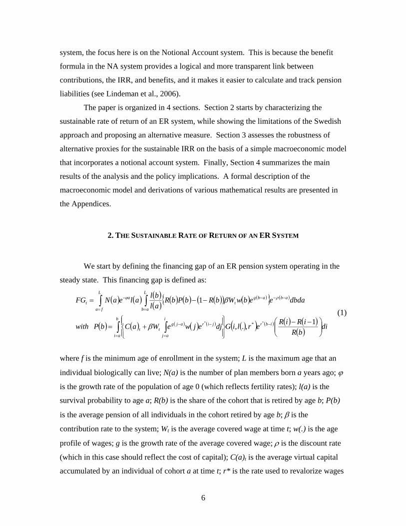
The sustainable IRR can be defined as the r* that solves FG(.)=0.7 There is no

close form solution to this equation, but one can see that r* will not only depend on the

growth rate of the average covered wage (g) and the growth rate of the population of new

borns (ϕ) – which in turn affects the growth rate of the population of contributors --, but

also survival probabilities and retirement patterns. To show this, Figure 1 graphs in the

(FG, r*) space various realizations of equation (1). Each line corresponds to a

combination of the growth rate of the average wage, the growth rate of the population,

retirement probabilities, and the distribution of wages. The intersection of each line with

the horizontal axis gives the equilibrium IRR. We see that the IRR increases with the

level of economic growth, the population growth rate, and the fall in retirement

probabilities by age. We also notice that a high rate of economic growth makes the lines

quite steep, indicating that small changes in the IRR on contributions can deviate the

system from its long-term equilibrium. As a corollary, for a given IRR, a small change in

the underlying macro and demographic conditions can also divert the system from

equilibrium. Clearly, outside the steady state the sustainable IRR would need to change

at each point in time. The question is how.

6 See Appendix 1 for the derivation of P(b). 7 We observe that what is required is that the contributions of current plan members are enough to finance all pensions assuming that reserves are invested at market prices – captured by the rate ρ. One could introduce new generations into account, but this would not change the nature of the problem. In this case we are looking at a sustainable cross-sectional IRR. With new generations one would be looking at a longitudinal IRR.

8

Figure 1: Financing Gap and the IRR

-20

-15

-10

-5

0

5

10

15

20

0.01 0.02 0.03 0.04 0.05N

PV(B

alan

ces)

/Wag

eBill

Baseline

Retirement age starts at 55 with 10% probability

GDP grows at 5% per year

Survival probabilities of year 2050

Population growth rate at 4%

GDP growts at 5% and population at 2.5%

GDP at 5%, population at 2.5%, and retirement age starts at 55 with 10% probabiliy

Note: The baseline scenario is built over the following assumptions: population growth of 1% per year; GDP growth of 3% per year; 2% growth in wages between ages; survival probabilities for Morocco in 2004; minimum retirement age 40 with 1% probability and maximum retirement age 75; no dropouts within age cohorts. The other lines represent deviations in one of the parameters from the baseline. Source: Authors’ calculations

The proposal developed here is based on an accounting framework “a la Swedish”

-- although as shown below the actual indexation mechanism used in Sweden is not fully

consistent with this underlying framework. The idea is simple: choose the IRR at each

time t in a way that guarantees that the liabilities of the pension system are equal to its

assets. The trick then is to properly define these liabilities, and in particular, the assets of

the ER pension system with pay-as-you-go financing.

The assessment of the liabilities of the system is straight forward. They are given

by the present value of future pension payments to current retirees and to current

contributors based on rights accrued to date.8 In the case of a notional account system the

value of the IPD is easily defined. It is given by the capital accumulated in the individual

accounts plus the pensions in payment by age cohort multiplied by the annuity factor for

that cohort.

8 The pension system liability definition here corresponds to the “gross implicit pension debt I” definition of Holzmann, Palacios and Zviniene (2001).

9

The definition of assets is less intuitive. Clearly, a portion of the assets is given

by the ¨reserves¨ of the pension plan – which can be equal to zero. The other part is the

so called pay-as-you-go asset which is defined as the present value of future contributions

minus the present value of pensions ensuing from these contributions (see Valdés-Prieto,

2005a; and Robalino and Bogomolova, 2005). The pay-as-you-go asset is positive when

the implicit rate of return on contributions paid by the ER pension plan is below the rate

used to discount future cash-flows. This rate can be approximated by the rate of return

that the pension institution receives on the investments of the buffer fund (a market rate).

The difference between this rate and the implicit rate of return on contributions can be

interpreted either as the “opportunity cost” of saving in the ER plan or, put in other terms,

an implicit tax on savings. Thus, in an ER system that is very generous, meaning it pays

an IRR above market, the pay-as-you-go asset is negative.

Formally, in a solvent ER pension system with pay-as-you-go financing the

following equality needs to hold:

ttt FPAIPD += , (2)

where IPDt is the implicit pension debt at time t; PAt the pay-as-you-go asset and Ft the

value of the reserves (financial assets). So in summary, in a solvent pension system, the

pension promises that have been made to date have to be backed by financial assets and

the future contributions net of pension rights accruing from them. As discussed above, a

pension plan can operate with a negative pay-as-you-go asset, but not forever.

From equation (2) it follows that given the growth rate of the pay-as-you-go asset,

call it a, and the growth rate of the reserves, call it r, one can solve for the allowable

growth rate of the IPD at time t, holding constant system, economic, and demographic

conditions. It turns out that this allowable growth rate of the IPD is the IRR that the

pension system can afford to pay on contributions. It is the rate by which the pension

plan can revalorize wages and index pensions. Indeed, as explained before, the IPD is

made of accumulated contributions plus pensions in payment multiplied by the

appropriate annuity factor. So the growth rate of the IPD is given by the growth rate of

the stock of contributions and the stock of pensions in payments.

Thus, the IRR at time t can then be defined as:

10

t

ttt

t

t

t

tt IPD

IPDFPArIPD

FaIPDPAIRR −+

++= (3)

Hence, if one is able to obtain an accurate and simple estimate of the PA at each point in

time, the expected sustainable IRR can be easily computed.

Before presenting a possible measure for the PA, we discuss how the approach

proposed here to estimate the sustainable IRR differs from the Swedish system.

The analytical framework for the Swedish automatic stabilization mechanism is

developed in Settergren and Mikula (2005). The authors start by dividing the cross-

section financing gap of the pension system (a simplification of equation 1) by total

contributions. In doing so, the authors indicate that they approximate the total financing

gap that can be supported by one unit of contribution. The authors call this ratio the

turnover duration (TD) and show, under simplifying assumptions, that the TD is equal to

the money weighted average age of retirees minus the money weighted average age of

contributors. The turnover duration times the contribution base then provides an estimate

of what they call the contribution asset – different from the pay-as-you-go asset concept

discussed above. Given information about the value of reserves, the authors calculate the

“total assets” of the system. When assets are equal or above pension liabilities,

contributions/pensions are revalorized/indexed by the growth rate of the covered average

wage. The indexation factor for pensions is also adjusted to take into account the interest

rate imputed in the calculation of the annuity factors (see next section). When assets fall

below liabilities a “balancing mechanism” is activated and the growth rate of the average

covered wage is multiplied by the funding ratio. Formally, we have:9

⎟⎟⎠

⎞⎜⎜⎝

⎛−

⎭⎬⎫

⎩⎨⎧

⎟⎟⎠

⎞⎜⎜⎝

⎛ +=

−

11,min1t

t

t

tttt W

WIPD

FCTDIRR , (4)

9 We emphasize that this description of the Swedish NDC system does not follow from the framework developed in Settergren and Mikula (2005). If one applies the framework rigorously, the rate used to revalorized accounts and index pensions would be simply given by:

( )⎟⎟⎠

⎞⎜⎜⎝

⎛−

+= +

+ 1. 11

t

t

t

tttt W

WIPD

FCTDIRR.

11

where Wt is the average covered wage at time t. Basically, the IRR is equal to the

funding ratio multiplied by the growth rate of the average covered wage. If the funding

ratio falls below one, then pensions and wages are indexed by less than the growth rate of

the average covered wage (at least in the initial stage of “balancing”). 10

The same IRR is used to index pensions, but it is adjusted to take into account the

discount rate imputed in the calculation of the annuity. Pensions are indexed by:

( )( ) 11

1' −+

+=

iIRR

IRR tt , (5)

where i is the discount rate imputed in the calculation of the annuity.11

There are several issues with this proposed balancing mechanism. A first issue is

that the mechanism does not follow from first principles. It is unclear why an equation

such as (4) was used instead of equation (3), where PA would have been replaced by

TD*C. The second issue relates to the interpretation of the turnover duration.

Mathematically, the TD is not a good approximation of the pay-as-go-asset, which is the

relevant concept. For instance, the TD can increase as a result of an increase in life

expectancy and that would be perceived as an increase in contribution assets when in fact

that increase can reduce the pay-as-you-asset as individuals receive pensions for longer.

It is also not clear why the TD would provide an estimate of the financing gap that can be

supported by a given contribution base. It could be informative regarding the level of the

financing gap, but not necessarily whether it is sustainable. Actually, if the system is

solvent one would like the financing gap to be zero: liabilities would equate financial

assets plus the pay-as-you-go asset. Finally, as the authors emphasize, the calculation of

the TD is based on current information and the assumption of constant population

growth. The TD would not capture future changes in the contribution base and therefore

could overestimate or underestimate assets, thus paying an IRR on contributions that is

too high or too low. In fact, Settergren (2001) admits that long-term deficits in the buffer

fund can arise in the case of long-term strains on the system like negative population

10 In fact, the Swedish indexation mechanism works somewhat differently allowing the indexation to be higher than the growth rate of the average covered wage in a “recovery stage” when the balancing mechanism is active. The formula above is a simplification; however, the programming of our projections is based on the true system rules. 11 i=0.016 under the rules of the Swedish system.

12

growth. Section 4 will show that this is indeed what happens in the presence of

exogenous shocks.

If the TD is to be replaced, how would the PA is computed? In the proposed

approach, computing the PA is not very different from computing the IPD – which is also

required in the Sweden scheme. For the IPD, one needs estimates of G factors (annuity

factors) by age. These depend on survival probabilities by age and assumptions about the

future indexation of pensions (see discussion below on the discount rate used in the

formula). For the PA, one needs estimates of what we call Z factors -- to keep similar

terminologies -- that give net assets for each age cohort. These Z factors also depend on

survival probabilities and the market discount rate, but in addition estimates of

retirement/dropout probabilities, the current age profile of wages (also used for the

calculation of the TD), and the expected growth rate for wages. So computing the

expected PA is not more difficult than computing the TD or the IPD.

The Z factor for a cohort of age i at time t, is given by:

( ) ( ) ( ) ( ) ( )( ) ( ) ( )

( )

( )( )

( )( ) ( )

( )

( )( )

( )( )∑

=

+

−

−

⎪⎪⎪

⎭

⎪⎪⎪

⎬

⎫

⎪⎪⎪

⎩

⎪⎪⎪

⎨

⎧

⎟⎟⎟⎟⎟⎟⎟⎟

⎠

⎞

⎜⎜⎜⎜⎜⎜⎜⎜

⎝

⎛

⎟⎟⎠

⎞⎜⎜⎝

⎛⎟⎟⎠

⎞⎜⎜⎝

⎛ +−+⎟⎟

⎠

⎞⎜⎜⎝

⎛ +−

⎥⎥⎥⎥⎥

⎦

⎤

⎢⎢⎢⎢⎢

⎣

⎡

⎟⎟⎠

⎞⎜⎜⎝

⎛++

−

⎟⎟⎠

⎞⎜⎜⎝

⎛++

−⎟⎟⎠

⎞⎜⎜⎝

⎛++

++

+−⎟⎟

⎠

⎞⎜⎜⎝

⎛++

=L

ia

B

ai

i

a

ia

A

ia

t adad

avav

rEg

rEg

rEg

grEg

idiviladavaliwWtiZ

4444444444444444 34444444444444444 21

43421

1111

111

11

11

1]1[

11

11,

*

1

***

ρρβ

(5)

where v (a) gives the probability of not being retired by age a, d (a) the probability of not

having dropped out of the system by age a, and E(r*) gives the expected rate of return on

contributions. Basically, expression A captures the present value of contributions paid at

age a, and expression B the pensions (and lump sum) paid to new retirees (and dropouts)

at age a.12 Then the pay-as-you-go asset at time t is:

( ) ( ) ( ) ( ) ( )∑∑∑+= ==

Δ+=T

tk

L

fb

L

fat kbZkbNtaZtaNPAE

1

,,,, , (6)

where N (a,t) are the contributors of age a at time t, dN (b,k) the new entrants of age b at

time k, and T the planning horizon.

One can argue that having estimates of future entrants, the growth rate of the

average wage, and the expected rate or return on contributions is complicated. The 12 See Appendix 1 for the derivation of Z (i,t).

13

proposal developed here assumes that past trends hold. The E(r*) is estimated by an

average of past IRRs and new contributors by age can be projected given past

information on new entrants and their age distribution. A virtue of the PA is that it is

forward looking. Basically, it tries to anticipate the effects of shocks that occur today on

the future flows of net contributions. Clearly, the past is not necessary a good predictor

of the future. Hence, when calculating the PA of a system in year 2005, one would miss

the impact of unknown phenomena that take place, say, one decade from now. Let us

assume, for instance, that the unknown shock is a permanent drastic drop in coverage

rates that takes place suddenly – unannounced. Estimates of the PA in the years prior to

the shock would overestimate its true value (i.e., wages and pensions would be

revalorized/indexed by a rate that is too high). Nonetheless, as soon as the shock takes

place, and the system identifies that is permanent, its short and long-term effects would

be incorporated in the calculation of the IRR, making up for previous over adjustments.

We also emphasize that those shocks that take place far into the future have a small

impact in the current value of the PA.

Computing annuities and indexing pensions13

There is an important precision to be made regarding the calculation of annuity

factors and the type of indexation mechanism used for pensions. Often decisions at these

two levels are disconnected and, as shown in Section 4, this is problematic for an NA

system without the appropriate stabilization mechanism.

If in practice pensions are going to be indexed by the IRR (or rough proxies such

as wages or GDP growth rates), which is also the rate used to revalorize wages, then the

annuity factor should not incorporate a discount rate. In other words, the pension would

be simply equal to the notional capital accumulated in the individual account divided by

the life expectancy at retirement. On the contrary, if pensions are solely going to be

indexed by prices, the annuity factor should incorporate in the calculation the expected

IRR. Basically, if pensions are only going to be indexed by prices then they should be

13 This is not an issue if the public pension system only manages the accumulation phase and then outsources the issuance of annuities. Basically, upon retirement individuals would receive a lump sum and then have the mandate to purchase an annuity in the private sector. Alternatively, the pension fund could conduct biddings among private sector providers to allocate cohorts of annuitants.

14

higher from the start. If they are going to be indexed by the IRR then they should be

smaller.

It is possible to define the correct indexation factor π given the sustainable

IRR and the discount rate i used in the calculation of the pension. Factor π needs to

solve:

( )( )( ) RRb

RbMax

RbMax

Rb

Rb

R CIRR

bRs

ibRs

C=

++

⎟⎟⎟⎟

⎠

⎞

⎜⎜⎜⎜

⎝

⎛

+−

−

+=

+=

−−∑

∑)(

)(

1

1

)( 1),(1

1),(

π , (7)

where CR is the capital accumulated in the individual account at the time of retirement.

The expression in brackets is the value of the initial pension calculated on the basis of a

discount rate i. Equation (7) states that if, ex-post, the pension is going to be indexed by

π the present value should still be equal to CR. It is easy to show that for equation (7) to

hold, the following needs to be verified for any b:

11

11

111

−⎟⎠⎞

⎜⎝⎛

++

=⇔

+=

++

iIRR

iIRR

π

π

. (8)

Clearly, if the IRR itself is not sustainable, then this correction will not solve the problem

of financial sustainability.

In practice, policymakers would need to adopt an indexation mechanism that is

consistent with the annuity formula but this is seldom the case. Introducing a discount

factor in the calculation of the annuity is a way to guarantee higher pensions up front. At

the same time policymakers might face pressure to keep the growth of pensions in line

with the growth in wages.

If the system incorporates a stabilization mechanism such as equation (3), then

there is flexibility in terms of whether or not a discount factor is used in the calculation of

the annuity. Indeed, the stabilization mechanism will ensure that the IRR that is used to

revalorize wages and index pensions after the discount factor was taken into account

brings the pension system to a sustainable path. The higher the discount rate used in the

calculation of the annuity, the lower the IRR that the system will pay (i.e., the lower the

15

rate used to revalorize and index pensions). If no discount factor is used, then the system

will pay the maximum IRR other things being constant. Because the IRR is the rate that

should be used to discount the flow of contributions and pensions, this approach ensures

that all individuals within a given age-cohort receive the same implicit rate of return on

their contributions – albeit one that moves over time – regardless of wages and

contributions histories.

With no stabilization mechanism, however, the discount factor might be too high

relative to the allowable IRR – which as seen before changes over time – and it will not

be possible to correct. This is shown in Section 4. One alternative in this case, is not to

include a discount factor in the calculation of the annuity, but to guarantee full indexation

of pensions on the basis of the system IRR. However, it can be shown that under general

conditions individuals – at least those who have limited access to financial markets and

face stringent borrowing constraints - would be better off if a discount rate is introduced

up front and the pensions are indexed by prices.14

3. SIMULATING THE ROBUSTNESS OF ALTERNATIVE RULES FOR THE IRR OF THE SYSTEM

To study the dynamics of an ER pension system with pay-as-you-go financing

under alternative rules for the IRR, we use a simple one sector macro model that

incorporates a notional account pension scheme (see Appendix 2 for a formal

description). For simplicity, and given that the focus is to analyze the dynamics of the

IRR, economic growth and the savings rate of the economy are exogenous in the model.

Future extensions should study the behavior of the pension system with endogenous

savings. The dynamics of wages and the market interest rate, on the other hand, are

endogenous in our model. This model provides a mechanism to ensure internal

consistency regarding changes in pension system design, macroeconomic trends and

demographic trends. For instance, simulated fluctuations in GDP growth will affect the

pension system through changes in wages and the interest rate – a recession is

accompanied by higher interest rates. Similarly, retirement and survival probabilities will 14 This statement holds if capital market participation constraints diminish the opportunity for intertemporal consumption-saving optimization and we accept the general individual utility optimization framework to assess welfare implications. A proof of this claim is available from the authors...

16

affect the economy through a change in the size and age composition of the labor force,

which in turn affects wages and the interest rate. Coverage and labor supply, however,

are not affected by changes in the macro economy or pension system parameters.

We use the model to understand how various rules for the evolution of IRR on

contributions affect the dynamics of the pension system. In particular, cash balances and

reserves levels. If the earnings-related system is financially self-sustainable, then the

value of reserves should never be negative – or at least not for an extended period of

time.

We consider 6 rules to determine the IRR across a large number of economic and

demographic scenarios: (i) wages are revalorized by the growth rate of the average

covered wage and pensions are indexed by prices (i.e., growth is zero in real terms); (ii)

the IRR is equal to the growth rate of the average covered wage and it applies to wages

and pensions; (iii) the IRR is equal to the growth rate of the covered wage bill; (iv) the

IRR is equal to the growth rate of GDP; (v) the IRR is based on the Swedish system

(equation 4); and (vi) the IRR is based on the proposal developed in this paper (equation

3).15 We also take into account two different methods to compute the annuity; with and

without a discount factor.

As for the scenarios, we consider combinations of eight blocks of variables: (i)

population growth; (ii) GDP growth; (iii) retirement probabilities; (iv) drop-out/reentry

probabilities; (v) survival probabilities; (vi) productivity by age; (vii) inflation and

interest rates; and (viii) the coefficient of human capital in the production function.

Basically, each of these variables/groups of variables is allowed to be in one out of three

states.16 The various states are described in Table 1 and have been selected to put the

pension system under high stress and assess its resilience. The deviations from state 1 can

be considered as shocks to the system. As a general rule, they are introduced at a point in

time when the system has already reached a great degree of maturity.

15 A paper by Lindeman et al. (2006) had analyzed the first 3 rules (with alternative combinations for wages and pensions), but outside a macro framework. The analysis here confirms some of the findings. 16 The probability of state 1 occurring is 50% for each of the blocks of variables. The probability of state 2 or 3 occurring is 25% respectively for each of the blocks of variables.

17

Table 1: State for Key Model Variables Variable(s) State 1 - Baseline State 2 State 3 Growth of

population of new born

Constant population (0% growth of population of new born.)

Population of new born initially remains constant, then decreases at an annual 0.5% rate between years 50 and 150, then it grows at 0.5% per year beyond year 150.

Population of new born initially remains constant, and then it gets on a steady decreasing path at an annual 0.5% rate beyond year 50.

GDP growth Real GDP grows at 2.5% per year.

Real GDP grows at 2.5% per year, then increases to 7% in year 150, then falls to 1% in year 165.

Real GDP grows at 2.5% per year, then a recession hits in year 150 (-5% per year). The economy recovers growth of 2.5% in year 155.

Retirement probabilities

Probability is zero up to age 39 then it increases linearly from 1% at age 40 to 100% at age 75.

Like state 1, but probability of retirement at age 40 increases from 1% to 30% in year 150; for other ages it is adjusted accordingly.

Like state 2, but the increase in the initial retirement probability does not happen through an immediate shock, but over a 30 year period.

Dropout/reentry probabilities

Dropout probabilities are zero at all ages.

Dropout probability for all ages suddenly increases to 30% in year 150 and then falls to 20% in year 155. The reentry probability is 10%.

Dropout probability for all ages suddenly increases to 30% in year 150 and then fall to 20% in year 160. The reentry probability is 10%.

Survival probabilities

Survival probabilities are constant over time at levels observed in Morocco today.

Survival probabilities increase to 1.5 times the expected 2050 levels for Morocco by year 150 of the simulation.

Survival probabilities increase to twice the expected 2050 levels for Morocco in year 150 of the simulation.

Productivity by age

Productivity increases at 2% for each year of age.

Productivity increases initially at 2% and then increases from 2% to 4% between years 100 and 110.

Productivity increases initially at 4% and drops from 4% to 1% between years 100 and 110.

Inflation and interest rates

Inflation at 2%. Real rate of return on reserves equal to 30%

Inflation at 2%. Real rate of return on reserves equal to 60%

Inflation at 2%. Real rate of return on reserves equal to 60%

18

of marginal productivity of capital. Discount rate and rate used to compute annuity set equal to long term GDP growth rate. Marginal return on capital equal to 1.25 times GDP growth.

of marginal productivity of capital. Discount rate and rate used to compute annuity set equal to long term GDP growth rate. Marginal return on capital equal to 1.25 times GDP growth.

of marginal productivity of capital. Discount rate and rate used to compute annuity set equal to long term GDP growth rate. Marginal return on capital equal to 2 times GDP growth.

Coefficient of human capital

Coefficient of human capital equal to 0.5.

Coefficient of human capital equal to 0.1.

Coefficient of human capital equal to 0.8.

Initial population of new born is 1,000. Initial GDP per capita is 100 units. Initial level of capital is calibrated to achieve targeted, long term, marginal return on capital. Minimum age to enter the labor force (f) set at 20 years

We discuss the results of the simulations in three parts. First, we look at the

dynamics of funds reserves under each of the rules for the IRR across a random sample of

100 scenarios evolving over a period of 300 years. Then, for each of the indexation rules,

we look at the distribution of the following outputs: (i) the value of the reserves as a share

of GDP in year 150 and year 300; (ii) the value of the cash-balance as a share of GDP in

year 150 and in year 300; (iii) the average IRR for the period t∈ [150,300]; and (iv) the

maximum value of the reserves as a share of GDP during the entire simulation period.

Finally, we analyze the sensitivity of the steady level of fund reserves and the IRR to

changes in selected model variables.

We first discuss the simulations where the calculation of the annuity factor does

not include a discount rate. The results show that only the new proposal developed in

this paper and the “price indexation mechanism” -- that is salaries (contributions)

revalorized by the growth rate of the covered average wage and pensions indexed by

inflation -- are capable of avoiding extended periods of negative reserves (see Figure 2).

Like the other revalorization/indexation mechanisms, however, price indexation is not

stable in the sense that for some of the scenarios, assets (reserves) accumulate without

bound. This implies that the system is penalizing workers by paying an IRR below the

sustainable level, essentially, a higher implicit tax on savings than what the system

requires.

19

This being said, none of the indexation mechanisms are systematically

unsustainable when the annuity is calculated without discounting, simply because there is

“more room” in this case to index pensions. The average value of reserves over the 100

random combinations of states is positive for all the 6 indexation mechanisms both in

year 150 and 300. The mean cash balance is positive for all the indexation mechanisms in

year 300, and positive or slightly negative in year 150 when some of the shocks take

effect (see Table 2).

The Swedish mechanism clearly outperforms the average wage growth, the

covered wage bill growth and the GDP growth indexation mechanisms in terms of

keeping positive reserves. However, the Swedish system exhibits a tendency to over

accumulate assets when population growth is positive, while the balancing mechanism is

vulnerable against a shrinking population. Indeed, several combinations of states that

include long-term negative population growth put the Swedish system into an

unsustainable path (see the Appendix 3 for a comparative sensitivity analysis of the

Swedish system and the new proposal including various population growth scenarios).

As pointed out already, the inflation adjustment rule is robust as pensions are

indexed, on average, by an IRR below the sustainable level. In a way, the protection

against “system bankruptcy” comes at the cost of high implicit taxes on savings. We also

notice that price indexation displays a higher variance in the level of reserves.

The proposal developed in this paper is the only mechanism that avoids extended

periods with negative reserves and converges towards a sustainable steady-state in all the

scenarios.

20

Figure 2: Dynamics of the Reserves/GDP Ratio When Annuity Does Not Include a Discount Rate

Prices Covered average wage

Covered wage bill GDP

Swedish system Equation (3)

Source: Author’s calculation.

When a discount rate is introduced in the calculations of the annuity the results

are very different (see Figure 3).17 The average wage growth, the covered wage bill

growth and the GDP growth indexation mechanisms become unsustainable in all the

scenarios. This is not surprising since, in essence, pensions are being indexed twice.

First, ex-ante, at the time of calculating the pension – since the annuity factor already

incorporates a discount (i.e., indexation) factor – then each time pensions are paid. 17 The discount rate that we use is equal, as is the standard assumption, to the long-term growth rate of GDP.

21

Price indexation behaves better since, as discussed in the previous section, the

calculation of the annuity with a discount factor (expressed in real terms), is consistent

with price indexation. The problem is that the discount rate used in the calculation of the

annuity factor is not necessarily the sustainable rate. Price indexation therefore struggles

with the higher level of initial pensions without any mechanism for correction.

Only the Swedish indexation mechanism and the new proposal based on

equation (3) are equipped to adjust the indexation mechanism in relation to the discount

factor used in the calculation of the annuity. The Swedish mechanism, when the

balancing mechanism is not activated, actually behaves like price indexation if the

growth rate of the average wage is equal to the discount rate used in the calculation of the

annuity factor. The stabilization mechanism, however, is not sufficient to deal with

periods of negative population growth rate and therefore there are still scenarios where

the reserves of the system become negative

The rule proposed in this paper, on the other hand, never generates negative

reserves and converge in all cases to a stable steady state. In part, this is because the

proposed algorithm also takes into account the impact of the discount rate in the pay-as-

you-go asset (i.e., other things being equal, the higher the discount rate the lower the pay-

as-you-go asset).

22

Figure 3: Evolution of the Reserves/GDP Ratio when the Annuity Includes a Discount Rate

Prices Covered average wage

Covered wage bill GDP

Swedish system Equation (3)

The discount rate used in the calculation of the annuity is equal to the long-term

growth rate of the economy. Source: Author’s calculations. `

To gain more insights into the results of the simulations, we look at summary

statistics for key output variables (see Table 2). There are several interesting

observations. First, the mechanism proposed in this paper and the price indexation

mechanisms are the only ones capable of ensuring positive reserves levels at the end of

the simulation horizon. Even the Swedish system runs into debt by year 300 in the

amount of 57.2% of GDP under the worst set of “environment conditions.” We also

23

observe that both the range and the variance of the level of reserves are the smallest under

the indexation rule following equation (3). The proposed mechanism “downward adjusts”

the IRR in straining situations, but even then it does not push the IRR into the negative.

This is an important message from the simulations because, conceptually, negative IRR

paths are consistent with equation (3) under certain circumstances. These, however,

would be difficult to implement at the practical level.

Table 2: Descriptive Statistics for Selected Outputs

Annuity calculated with

discounting Annuity calculated without

discounting Mean Stdev Min Max Mean Stdev Min Max Average wage

Reserves/GDP t=150

-1.326 0.698 -2.480 -0.146 0.918 1.283 -0.050 4.341

Reserves/GDP t=300

-3.390 3.514 -17.241 -0.728 0.761 2.331 -1.301 8.856

Balance/GDP t=150

-0.031 0.013 -0.046 -0.009 -0.002 0.006 -0.008 0.004

Balance/GDP t=300

-0.022 0.017 -0.065 0.001 0.000 0.006 -0.012 0.013

Average IRR (to year 300) 0.021 0.005 0.009 0.032 0.021 0.005 0.009 0.032

Wage bill Reserves/GDP

t=150 -

0.959 0.561 -1.689 -0.124 1.180 1.400 0.277 4.823 Reserves/GDP

t=300 -

2.765 3.036 -15.027 -0.366 1.207 2.644 -0.557 9.164 Balance/GDP

t=150 -

0.023 0.010 -0.030 -0.009 0.004 0.000 0.003 0.004 Balance/GDP

t=300 -

0.020 0.013 -0.044 -0.004 0.002 0.001 0.001 0.004 Average IRR (to

year 300) 0.025 0.006 0.016 0.038 0.025 0.006 0.016 0.038 GDP

Reserves/GDP t=150

-0.959 0.561 -1.689 -0.124 1.180 1.400 0.277 4.823

Reserves/GDP t=300

-3.255 3.150 -15.027 -0.794 0.850 2.535 -1.993 9.164

Balance/GDP t=150

-0.023 0.010 -0.030 -0.009 0.004 0.000 0.003 0.004

Balance/GDP t=300

-0.020 0.013 -0.044 -0.004 0.002 0.001 0.001 0.004

Average IRR (to 0.022 0.004 0.016 0.025 0.022 0.004 0.016 0.025

24

year 300) Inflation

Reserves/GDP t=150 1.191 1.142 0.297 4.058 2.706 2.113 1.146 8.115

Reserves/GDP t=300 0.928 2.102 -0.691 8.262 3.734 5.657 0.509 19.952

Balance/GDP t=150 0.005 0.009 -0.007 0.020 0.024 0.003 0.019 0.028

Balance/GDP t=300 0.001 0.002 -0.003 0.008 0.016 0.009 0.004 0.033

Average IRR (to year 300) 0.021 0.005 0.009 0.032 0.021 0.005 0.009 0.032

Swedish mechanism

Reserves/GDP t=150 0.859 1.187 -0.040 4.028 0.928 1.295 -0.046 4.381

Reserves/GDP t=300 0.947 2.136 -0.471 8.270 0.968 2.254 -0.517 8.930

Balance/GDP t=150

-0.001 0.005 -0.007 0.004 -0.002 0.006 -0.008 0.004

Balance/GDP t=300 0.002 0.004 -0.009 0.012 0.002 0.005 -0.011 0.013

Average IRR (to year 300) 0.019 0.006 0.002 0.030 0.019 0.006 0.002 0.030

Equation 3 Reserves/GDP

t=150 1.381 0.196 1.057 1.841 1.548 0.280 1.102 2.176 Reserves/GDP

t=300 1.057 0.460 0.498 1.851 1.203 0.533 0.572 2.266 Balance/GDP

t=150 0.019 0.012 -0.007 0.036 0.021 0.012 -0.009 0.037 Balance/GDP

t=300 0.008 0.008 -0.008 0.021 0.008 0.009 -0.009 0.025 Average IRR (to

year 300) 0.002 0.006 -0.007 0.0164 0.014 0.007 0.003 0.0305 Source: Authors’ calculations.

To better understand the interactions between the macro economy and the pension

system under the Swedish and the proposed indexation mechanisms we simulated the

effects of isolated changes in selected model variables on the steady-state levels of the

fund reserves, cash balances, the path of the funding ratio and the IRR. The results are

presented in Appendix 3. The main messages from the analysis can be summarized are

follows.

25

First, it is interesting to observe that the Swedish system generates higher funding

ratios than the proposal developed in this paper. This reflects the difference in the

methodology used to calculate the pay-as-you-go asset. The new proposal implements a

direct estimation of this asset. The Swedish system approximates this asset through the

level of contributions and the turnover duration. The results suggest that this

methodology tends to overestimate the pay-as-you-go asset.

Second, the new proposal generates more rapid adjustment paths in response to

shocks. Fluctuations in adjustment paths are also less pronounced than in the case of the

Swedish system. This is because the Swedish system is sensitive to changes in the

growth rate of the covered average wage, which is in turn very sensitive to economic

shocks. The new proposal relies on the pay-as-you-go asset which dampens these

fluctuations by also taking into account the effects on the dynamics of the population of

contributors and beneficiaries.

Third, the Swedish system is very sensitive to changes in the growth rate of the

population and there are cases where the system is not able to avoid negative reserves.

This can also be explained, in part, by a revalorization based on the growth rate of the

covered average wage, which will be higher when population growth rates – and

therefore the growth rate of the labor force – fall.

Finally, while the funding ratio falls when retirement probabilities, drop-out

probabilities, and survival probabilities increase, the reduction is not always sufficient to

activate the balancing mechanism. This implies that the revalorization continues to

depend on the growth rate of the covered average wage and that pensions are indexed by

the growth rate of the average wage adjusted by the discount factor. When retirement

probabilities increase, wages and the IRR go up – since labor supply falls. When survival

probabilities increase, wages and the IRR go down – since the labor force increases.

Only when the shock is driven by an increase in drop-out probabilities, which is less

important for the dynamics of wages, at least in the short term, the IRR is more

responsive to the funding level.

By looking at the IRRs generated by the Swedish system one can see that these

are often above the IRRs generated by the new proposal, which as shown in the previous

section, preserve the solvency of the system (i.e., liabilities are equal to assets).

26

The dynamics of the pension plan under the Swedish stabilization mechanism

deserves further analysis. As previously discussed, the IRR paid by the system is roughly

equal to the funding ratio times the growth rate of the average wage – when the balancing

mechanism is on. The funding ratio in turn depends on the turnover duration that, when

multiplied by total contributions, is supposed to provide an estimate of the assets of the

plan – excluding the reserves. Because the turnover duration depends on average

contributions and average pensions by age, it is sensitive to changes in retirement and

dropout probabilities. It is also sensitive to changes in the age-wage profile and shocks

that affect the marginal productivity of labor. Figure 4 displays the evolution of the

turnover duration across the same 100 scenarios presented above. We observe that for

several of the scenarios, those where macroeconomic, behavioral, and/or demographic

shocks are observed, the TD is subject to important changes. These fluctuations,

however, are often positive indicating a higher level of assets. Therefore, for several of

the shocks assets would actually increase and the balancing mechanism would not be

activated.

Figure 4: Dynamics of the Turnover Duration in the Swedish Stabilization System Annuity with discount factor Annuity without discount

factor

Source: Authors’ calculations.

27

4. DISCUSSIONS AND POLICY IMPLICATIONS

In this paper we have proposed a mechanism to design a financially sustainable

and secure earnings related scheme with pay-as-you-go financing. The mechanism uses a

new measure for the rate that the plan should use to revalorize contributions and index

pensions (i.e., the sustainable implicit rate of return on contributions). This rate is a

function of the growth rate of the reserves (in this case the stock of government bonds)

and the so called pay-as-you-go asset of the system.

While the proposed arrangements could serve any ER system, they are better

suited for notional account systems that establish a clear link between contributions, the

rate of return on these contributions, and pensions. In addition, this system has a simple

characterization of the IPD: the sum of notional capital in the individual accounts, plus

pensions in payment by age cohort times the annuity factor of that cohort.

There are, however, issues that could affect implementation and that deserve

further attention. A first set of issues has to do with the mechanism used to compute the

IRR on contributions. One is that the value of the pay-as-you-go asset will depend on

expectations about the initial IRR and the growth rate of wages – this could give room to

discretion. The second is that financial sustainability might require that in some

circumstances the IRR be negative. Since this rate is used to index pensions the approach

would require that individuals accept the possibility of having their pensions drop in

absolute terms. This is unlikely to be appealing to individuals. One way around this is to

have pension which are only indexed by inflation but that in the calculation include an

implicit interest rate. The stabilization mechanism suggested here would then ensure that

the IRR paid on contributions is properly adjusted.

Another question is the level of sophistication of the scheme. Some might

consider that the proposed method to compute the IRR is complex and that pensions

systems in middle and low income countries will not have the institutional capacity to

implement. Our position is that creating this institutional capacity should be part of any

reform program -- including one that intends to keep defined benefit provisions intact. In

all cases, information and administrative systems should be upgraded to ensure that the

28

pension fund can properly track the contributions of plan members and other individual

characteristics. In all cases the managers of the pension plan should have access to up to

date financial information including the evaluation of the liabilities of the plan.

REFERENCES:

Auerbach, Alan J. and Laurence J. Kotlikoff. 1987. Dynamic Fiscal Policy, Cambridge University Press. Borensztein, Eduardo and Paolo Mauro. 2004. “The Case for GDP-Indexed Bonds.” Economic Policy, 19 (38), pp. 166-216. Buchanan, James M. 1968. “Social insurance in a growing economy: a proposal for radical reform.” National Tax Journal, 21, December: 386-39. Cichon, M. 1999. “Notional defined-contribution schemes: Old wine in new bottles.” International Social Security Review, 52 (4): 87-105. Devolder, P. 2005. “Le financement des régimes de retraite.” Economica, Paris. Holzmann, Robert, and Edward Palmer, eds. 2006. “Pension Reform: Issues and Prospects for Non-Financial Defined Contribution (NDC) Schemes.” World Bank. Washington DC. Holzmann, Robert, Robert Palacios, and Asta Zviniene. 2001. “On the Economics and Scope of Implicit Pension Debt: An International Perspective.” Empirica, 28: 97-129. Lindeman, David, David Robalino, and Michal Rutkowski. 2006. “NDC Pension Schemes in Middle- and Low-Income Countries.” In Robert Holzmann and Edward Palmer, eds., Pension Reform: Issues and Prospect for Non-Financial Defined Contribution (NDC) Schemes. World Bank. Washington DC. Palacios, Robert and Yvonne Sin. 2002. “Pension Policy Options in Eritrea.” Report No. 28541-ER, Poverty Reduction and Economic Management 2, Country Department 5, Africa Region. World Bank. Washington DC. Robalino, David, Edward Whitehouse, Anca Mataoanu, Alberto Musalem, Elisabeth Sherwood, Oleksiy Sluchinsky. (2005). Pensions in the Middle East and North Africa Region: Time for Change. World Bank. Washington DC.

29

Robalino, David, and Tatyana, Bogomolova. 2006. “Implicit Pension Debt in the Middle East and North Africa: Magnitude and Fiscal Implications.” Middle East and North Africa Working Paper Series No. 46, World Bank. Washington DC. Robalino, David, Richard Hinz, Oleksiy Sluchinsky, Mark Dorfman, and Anca Mataoanu. 2005. “Egypt: A Framework for an Integrated Reform of the Pension System.” Unpublished Report. World Bank. Washington DC. Settergren, Ole. 2001. “The Automatic Balance Mechanism of the Swedish Pension System – A Non-technical Introduction.” Stockholm: Swedish National Social Insurance Board. Settergren, Ole. ed. 2005. “The Swedish Pension System Annual Report.” Stockholm: Swedish Social Insurance Agency. Settergren, Ole, and Boguslaw Mikula. 2005. “The Rate of Return of Pay-as-You-Go Pension Systems.” In Robert Holzmann and Edward Palmer, eds., Pension Reform: Issues and Prospect for Non-Financial Defined Contribution (NDC) Schemes. World Bank. Washington DC. Sinn, H.W. (2000) “Why a funded pension is useful and why it is not”, International Tax and Public Finance 7: 389-410. Valdés-Prieto, Salvador. 2005a. ”Pay-as-you-go securities.” Economic Policy, 42, April: 215-251, London (CEPR). Valdés-Prieto, Salvador. 2005b. “A Market-based Social Security as a Better Means of Risk-Sharing.” Pension Research Council Working Paper 2005-16, Wharton School, Philadelphia.

30

APPENDIX 1 - DERIVATIONS

Derivation of P(b)

The average virtual capital accumulated by an individual of a cohort a at time t who

retires at age i with i ≤ b:

( ) ( ) ( ) ( )djejweWaCi

aj

jirajgtt ∫

=

−−+*

β (A1-1)

If we turn this virtual pension capital into an annuity, the average pension payment of an

individual of cohort a retiring at age i with i ≤ b in the period when the individual

reaches age b (i.e. at time t+b-i) is as follows:

( ) ( ) ( ) ( ) ( )( ) ( )ibri

aj

jirajgtt erliGdjejweWaC −

=

−−

⎪⎭

⎪⎬⎫

⎪⎩

⎪⎨⎧

+ ∫** *,.,β (A1-2)

Recall that R(b) is the share of the age cohort (any age cohort given constant retirement

probabilities) that retired by age b. Consequently ( ) ( )[ ] ( )bRiRiR 1−− is the share of R(b)

that is associated with those who retired between ages i-1 and age i. Consequently the

formula for the average pension payment at time t, calculated in relation to all individuals

in age cohort a who retire at or before age b, can be constructed by integrating the

previous formula over all retirement ages between a and b and including relative weights

of the population retired between ages i and i-1:

( ) ( ) ( ) ( ) ( ) ( )( ) ( ) ( ) ( )( ) dibR

iRiRerliGdjejweWaCabP ibrb

ai

i

aj

jirajgtt ⎟⎟

⎠

⎞⎜⎜⎝

⎛ −−

⎪⎭

⎪⎬⎫

⎪⎩

⎪⎨⎧

+= −

= =

−−∫ ∫1,.,,

** *β . (A1-3)

Derivation of Z (i,t), the Z factor

31

The present value of future contributions assuming that that age profile of wages function

w (.) is consistent with the average growth rate of the covered wage bill g on the

individual level is as follows:

( ) ( ) ( ) ( )( ) ( ) ( )∑

=

−

⎟⎟⎠

⎞⎜⎜⎝

⎛++L

ia

ia

tg

idiviladavaliwW

ρβ

11 . (A1-4)

The joint probability that an active person of age a either retires or drops out by age a+1

is [ ] [ ])()1(1)()1(1 adadavav +−++− . Assuming that the virtual pension capital to be

accumulated beyond age i is to be used to purchase an annuity at retirement/drop-out age

a, the present value of pension benefits to be earned through future contributions by age

cohort i is as follows:

( ) ( ) ( ) ( )( ) ( ) ( ) ∑∑

=

−∗−−

=

+++⎥

⎦

⎤⎢⎣

⎡⎟⎟⎠

⎞⎜⎜⎝

⎛ +−+⎟⎟

⎠

⎞⎜⎜⎝

⎛ +−

a

ij

jaijia

L

iat rEg

adad

avav

idiviladavaliwW ])[1()1(

)1(1

)()1(1

)()1(1

ρβ . (A1-5)

Based on (A1-4) and (A1-5) and applying the sum of geometric series formula we have

that

( ) ( ) ( ) ( ) ( )( ) ( ) ( )

( )

( )( )

( )( ) ( )

( )

( )( )

( )( )∑

=

+

−

−

⎪⎪⎪

⎭

⎪⎪⎪

⎬

⎫

⎪⎪⎪

⎩

⎪⎪⎪

⎨

⎧

⎟⎟⎟⎟⎟⎟⎟⎟

⎠

⎞

⎜⎜⎜⎜⎜⎜⎜⎜

⎝

⎛

⎟⎟⎠

⎞⎜⎜⎝

⎛⎟⎟⎠

⎞⎜⎜⎝

⎛ +−+⎟⎟

⎠

⎞⎜⎜⎝

⎛ +−

⎥⎥⎥⎥⎥

⎦

⎤

⎢⎢⎢⎢⎢

⎣

⎡

⎟⎟⎠

⎞⎜⎜⎝

⎛++

−

⎟⎟⎠

⎞⎜⎜⎝

⎛++

−⎟⎟⎠

⎞⎜⎜⎝

⎛++

++

+−⎟⎟

⎠

⎞⎜⎜⎝

⎛++

=L

ia

B

ai

i

a

ia

A

ia

t adad

avav

rEg

rEg

rEg

grEg

idiviladavaliwWtiZ

4444444444444444 34444444444444444 21

43421

1111

111

11

11

1]1[

11

11,

*

1

***

ρρβ

. (A1-

6)

32

APPENDIX 2 - THE MACRO MODEL

The formal description of the model is presented in Box A2-1. The various equations are

organized in five blocks: population; labor force; output, wages and interest rates; plan

members; and revenues and expenditures of the pension system. We briefly discuss each

of these blocks.

The first two equations define the dynamics of the population (N). Basically, the

population of new born is assumed to grow at an exogenously defined rate (λ). Given

survival probabilities by age, the total number of individuals in each age cohort is

computed at each point in time.

Equations (A2-3) and (A2-4) determine the evolution of the labor force (L) and

human capital (H) respectively. The labor force is made of all individual of age a≥f

(where f is the minimum economically active age) and who have not retired. Thus, in

equation (A2-3), v (a) is the probability of not being retired by age a. The implicit

assumption is that participation rates are 100% for all ages. This simplification does not

affect the results from the analysis. As for human capital, it is defined as the sum of the

labor force by age-cohort multiplied by their productivity/quality, which will affect the

level of wages by cohort. Thus, in equation (A2-4), ε(a) captures the age-wage profile.

Equations (A2-5) to (A2-11) determine output (Q), the savings rate of the

economy (s), capital (K), total factor productivity (A), wages by age (w(a)), and the

market interest rate rm. The underlying assumption is that output is generated by a Cobb-

Douglas function that incorporates human capital, physical capital, and total factor

productivity. The growth rate of output (g) is defined exogenously. The savings rate of

the economy is defined in a way that, in the steady state, the level of capital ensures that

the market interest rate (the marginal productivity of capital) equals gτ, where τ is

defined exogenously. This last parameter is basically the ratio between the real market

interest rate and the growth rate of GDP. So, (1- α)/ (gτ) is the capital output ratio.

Wages (by age) and the market interest rate are then computed under the assumption of

full employment as the marginal productivity of labor (by age) and capital respectively.

In equations (A2-6) to (A2-11), α is the share of human capital in production.

33

The evolution of the stocks of contributors (C), dormants (D; individuals who

stopped contributing but have pension rights), and old-age pensioners (O) are given by

equations (A2-12) to (A2-14). We assume that all individuals in the labor force join the

pension system at the beginning of the simulation (C(a,1)=L(a,1)) and that all new

entrants to the labor force join the pension system at time t>1 (C(f,t)=L(f,t)). From there

the stock of contributors, dormants, and old-age retirees respond to survival probabilities

l (.), dropping out probabilities d (.), reentry probabilities b (.), and the probability of

continuing in the labor force instead of retiring v (a). Notice that individuals, who drop

out of the pension system, do not drop out of the labor force. In this model, these

individuals continue working and earning a salary – they simply do not contribute.

Finally, equations (A2-15), (A2-16), and (A2-17) give the dynamics of the capital

value of the individual accounts and total pension expenditures for each age cohort, as the

total reserves of the system. The new symbols in these two equations are: r*, the

revalorization/indexation factor for wages/pensions (i.e., the internal rate of return on

contributions); β, the contribution rate; G(a,t,i) the annuity factor at age a and time, that

depends on the interest rate i (a policy parameter); and η which gives the rate of return on

investments of the reserves relative to the market interest rate.

The notional capital value of pension accumulation over a period for a given age

cohort incorporates the previously accumulated capital and its returns plus current

contributions of the surviving and not yet retiring portion of the given age cohort.

Equation (A2-15) takes into account that contributions are paid continuously throughout

the year. The total pension amount paid to an age cohort evolves from period to period in

accordance with (A2-16). The surviving portion of previously retired individuals of the

cohort will receive pensions indexed by the IRR and the accumulated pension capital of

new retirees is turned into annuities. The reserves of the pension system (A2-17) evolve

over time in accordance with the returns/borrowing costs on the previously available

reserves and the sum of the balances of current contributions and “newly exchanged”

pension annuities for all age cohorts. These balances are augmented by the investment

returns/borrowing costs assessed on their continuous flows during the applicable year.

34

Box A2-1: Model for Analysis of Robustness of Rules on IRRs Initial and total population by age-cohort:

( ) 11)1,0(),0( −+= tNtN λ , (A2-1)

( )( )altNtaN aλ+

=1

),0(),( , (A2-2)

Labor force by age cohort and human capital:

( ) ( ) ( )( )

( )( ) ( ) ( ) ( ) ( )tfNtfLfaaNaLav

aval

altaLtaL ,,;1,1,;11,1,1 =≥∀=++

=++ , (A2-3)

( ) ( ) ( );,∑=

=M

fataLatH ε , (A2-4)

Output, productivity, wages and interest rate:

( ) ( )( ) 111 −+= tgQtQ (A2-5)

αα −= 1)()()()( tKtHtAtQ (A2-6)

( )τα

τα −

=−

=11 g

gs (A2-7)

( ) ( ) ( ) ( ) ( ) ( )111;11 Qg

KtsQtKtKτα−

=−+−= (A2-8)

( ) ( ) ( ) 1)( −−= αα tKtHtQtA , (A2-9)

( ) ( ) ( ) ( ) ( )atKtHtAtaw εα αα −−= 11, , (A2-10)

( ) ( ) ( ) ( ) ( )( )tKtQtKtHtAtrm αα αα −=−= − 1)()1( (A2-11)

Contributors, dormants, and old-age pensioners:

( ) ( ) ( )( ) ( ) ( )

( ) ( ) ( )( ) ( ) ( ) ( ) ( ) ( )tfLtfCaLaCabal

altaDav

avadal

altaCtaC ,,,1,1,;1,11,1,1 ==+

+⎥⎦

⎤⎢⎣

⎡⎟⎟⎠

⎞⎜⎜⎝

⎛ ++−⎥

⎦

⎤⎢⎣

⎡ +=++ (A2-12)

( ) ( ) ( )( ) ( )( ) ( ) ( )

( ) ( )adal

altaCabal

altaDtaD 1,11,1,1 ++−

+=++ , (A2-13)

( ) ( ) ( )( ) ( ) ( )[ ] ( )

( )( )( ) ⎟⎟

⎠

⎞⎜⎜⎝

⎛ +−

+++

+=++

avav

alaltaDtaC

alaltaOtaO 111,,1,1,1 , (A2-14)

Individual accounts by age cohort, total pensions by age-cohort, and total reserves:

( ) ( )( ) ( ) ( ) ( )( )

( )( ) ⎥

⎦

⎤⎢⎣

⎡⎟⎟⎠

⎞⎜⎜⎝

⎛ +−

+−⎥

⎦

⎤⎢⎣

⎡⎟⎟⎠

⎞⎜⎜⎝

⎛+++=++

avav

alaltrtawtaCtrtaItaI 1111*

2)(1,,)(1,1,1

** β , (A2-15)

( ) ( )( ) ( )( )

( ) ( )( ) ( )( )

( )( )

( )itaGav

aval

altrtaI

alaltrtaPtaP

,1,1

1111,1)(1,1,1

*

*

++

⎟⎟⎠

⎞⎜⎜⎝

⎛ +−

++

++

+=++ , (A2-16)

( ) ( ) ( )( ) ( ) ( )( )( ) ( )

( )( )( )

( )∑=

⎟⎟⎠

⎞⎜⎜⎝

⎛+

⎥⎥⎥⎥

⎦

⎤

⎢⎢⎢⎢

⎣

⎡

++

⎟⎟⎠

⎞⎜⎜⎝

⎛ +−

++

−++−=M

fa

mm tr

itaGav

aval

alrtaItawtaCtrtRtR

2)(1

,1,1

1111,,,11 ηβη

(A2-17)

35

APPENDIX 3 – SENSITIVITY/ROBUSTNESS ANALYSIS

The following figures compare the sensitivity/robustness of the Swedish

automatic balance mechanism and that of the indexation mechanism of the proposal

developed in this paper towards certain demographic shocks holding all other factors

constant. The baseline simulation path scenario corresponds to state 1 in Table 1. The

deviating paths are identified in the figure legends and they correspond to the alternative

states defined in Table 1. The sensitivity analysis towards population growth and

survival patterns includes one additional path each. All the simulations here apply

annuity calculations with discounting.

36

Sensitivity Analysis – Population Growth Scenarios Evolution of the Reserves and Balance of the Pension System as a Share of the GDP,

the Funding Ratio and Dynamic Internal Rate of Return of the Pension System under the Swedish Automatic Balance Mechanism and the New Indexation Proposal Swedish automatic balance mechanism new proposal

37

Sensitivity Analysis – Survival Pattern Scenarios Evolution of the Reserves and Balance of the Pension System as a Share of the GDP,

the Funding Ratio and Dynamic Internal Rate of Return of the Pension System under the Swedish Automatic Balance Mechanism and the New Indexation Proposal Swedish automatic balance mechanism new proposal

38

Sensitivity Analysis – Retirement Probability Scenarios Evolution of the Reserves and Balance of the Pension System as a Share of the GDP,

the Funding Ratio and Dynamic Internal Rate of Return of the Pension System under the Swedish Automatic Balance Mechanism and the New Indexation Proposal Swedish automatic balance mechanism new proposal

39

Sensitivity Analysis – Drop-Out Probability Scenarios Evolution of the Reserves and Balance of the Pension System as a Share of the GDP,

the Funding Ratio and Dynamic Internal Rate of Return of the Pension System under the Swedish Automatic Balance Mechanism and the New Indexation Proposal Swedish automatic balance mechanism new proposal

Social Protection Discussion Paper Series Titles No. Title 0827 On the Financial Sustainability of Earnings-Related Pension Schemes with

“Pay-As-You-Go” Financing by David A. Robalino and András Bodor, July 2008 (online only) 0826 An Ex-Ante Evaluation of the Impact of Social Insurance Policies on Labor

Supply in Brazil: The Case for Explicit Over Implicit Redistribution by David A. Robalino, Eduardo Zylberstajn, Helio Zylberstajn and Luis

Eduardo Afonso, July 2008 (online only) 0825 The Portability of Pension Rights: General Principals and the Caribbean Case by Alvaro Forteza, May 2008 (online only) 0824 Pension Systems and Reform Conceptual Framework

by Robert Holzmann, Richard Paul Hinz and Mark Dorfman, September 2008 (online only)

0823 Mandated Benefits, Employment, and Inequality in a Dual Economy

by Rita Almeida and Pedro Carneiro, August 2008 (online only) 0822 The Return to Firm Investments in Human Capital by Rita Almeida and Pedro Carneiro, June 2008 (online only) 0821 Population Aging and the Labor Market: The Case of Sri Lanka by Milan Vodopivec and Nisha Arunatilake, August 2008 (online only) 0820 China: Improving Unemployment Insurance

by Milan Vodopivec and Minna Hahn Tong, July 2008 (online only) 0819 Management Information Systems in Social Safety Net Programs: A Look at

Accountability and Control Mechanisms by Cesar Baldeon and Maria D. Arribas-Baños, August 2008 (online only)

0818 Guidance for Responses from the Human Development Sectors to Rising

Food Prices by Margaret Grosh, Carlo del Ninno and Emil Daniel Tesliuc, June 2008

(Revised as stand-alone publication) 0817 Levels and Patterns of Safety Net Spending in Developing and Transition

Countries by Christine Weigand and Margaret Grosh, June 2008 (online only)

0816 Labor Regulation and Employment in India’s Retail Stores by Mohammad Amin, June 2008 (online only) 0815 Beyond DALYs: Developing Indicators to Assess the Impact of Public

Health Interventions on the Lives of People with Disabilities by Daniel Mont and Mitchell Loeb, May 2008 0814 Enforcement of Labor Regulation and Firm Size

by Rita Almeida and Pedro Carneiro, May 2008 (online only) 0813 Labor Markets Lending and Analytical Work at the World Bank: FY2002-

2007 by Milan Vodopivec, Jean Fares and Michael Justesen, May 2008 0812 Risk and Vulnerability Analysis in the World Bank Analytic Work: FY2000-

2007 by Valerie Kozel, Pierre Fallavier and Reena Badiani, May 2008 0811 Pension Lending and Analytical Work at the World Bank: FY2002-2007 by Richard Hinz, Melike Egelmelzer and Sergei Biletsky, May 2008 (online

only) 0810 Social Safety Nets Lending and Analytical Work at the World Bank:

FY2002-2007 by Margaret Grosh and Annamaria Milazzo, May 2008 0809 Social Funds as an Instrument of Social Protection: An Analysis of Lending

Trends - FY2000-2007 by Samantha De Silva and June Wei Sum, July 2008 0808 Disability & Development in the World Bank: FY2000-2007 by Jeanine Braithwaite, Richard Carroll, and Karen Peffley, May 2008 0807 Migration, Labor Markets, and Integration of Migrants: An Overview for

Europe by Rainer Münz, April 2008 (online only) 0806 Is the Window of Opportunity Closing for Brazilian Youth? Labor Market

Trends and Business Cycle Effects by Michael Justesen, April 2008 0805 Disability and Poverty: A Survey of World Bank Poverty Assessments and

Implications by Jeanine Braithwaite and Daniel Mont, February 2008

0804 Poverty Traps and Social Protection by Christopher B. Barrett, Michael R. Carter and Munenobu Ikegami,

February 2008 0803 Live Longer, Work Longer: Making It Happen in the Labor Market by Milan Vodopivec and Primoz Dolenc, February 2008 (online only) 0802 Disability in Kazakhstan: An Evaluation of Official Data by Ai-Gul S. Seitenova and Charles M. Becker, February 2008 (online only) 0801 Disability Insurance with Pre-funding and Private Participation: The Chilean

Model by Estelle James, Augusto Iglesias and Alejandra Cox Edwards, January

2008 0719 The Life-Course Perspective and Social Policies: An Issues Note by A.L. Bovenberg, November 2007 0718 Social Safety Nets and Targeted Social Assistance: Lessons from the

European Experience by Chris de Neubourg, Julie Castonguay and Keetie Roelen, November 2007

(online only) 0717 Informality and Social Protection: Preliminary Results from Pilot Surveys in

Bulgaria and Colombia by Franco Peracchi, Valeria Perotti and Stefano Scarpetta, October 2007

(online only) 0716 How Labor Market Policies can Combine Workers’ Protection with Job

Creation: A Partial Review of Some Key Issues and Policy Options by Gaëlle Pierre and Stefano Scarpetta, October 2007 (online only) 0715 A Review of Interventions to Support Young Workers: Findings of the Youth

Employment Inventory by Gordon Betcherman, Martin Godfrey, Susana Puerto, Friederike Rother,

and Antoneta Stavreska, October 2007 0714 Performance of Social Safety Net Programs in Uttar Pradesh by Mohamed Ihsan Ajwad, October 2007 0713 Are All Labor Regulations Equal? Assessing the Effects of Job Security,

Labor Dispute and Contract Labor Laws in India by Ahmad Ahsan and Carmen Pagés, June 2007

0712 Convention on the Rights of Persons with Disabilities: Its Implementation and Relevance for the World Bank

by Katherine Guernsey, Marco Nicoli and Alberto Ninio, June 2007 0711 Reaching the Poor and Vulnerable: Targeting Strategies for Social Funds and

other Community-Driven Programs by Julie Van Domelen, May 2007 0710 The Macedonia Community Development Project: Empowerment through

Targeting and Institution Building by Caroline Mascarell, May 2007 0709 The Nuts and Bolts of Brazil’s Bolsa Família Program: Implementing

Conditional Cash Transfers in a Decentralized Context by Kathy Lindert, Anja Linder, Jason Hobbs and Bénédicte de la Brière, May

2007 (online only) 0708 Globalization and Employment Conditions Study by Drusilla K. Brown, April 2007 0707 The Kosovo Pension Reform: Achievements and Lessons by John Gubbels, David Snelbecker and Lena Zezulin, April 2007 (online

only) 0706 Measuring Disability Prevalence by Daniel Mont, March 2007 0705 Social Safety Nets in World Bank Lending and Analytic Work: FY2002-

2006 by Annamaria Milazzo and Margaret Grosh, March 2007 (online only) 0704 Child Labor and Youth Employment: Ethiopia Country Study by Lorenzo Guarcello and Furio Rosati, March 2007 0703 Aging and Demographic Change in European Societies: Main Trends and

Alternative Policy Options by Rainer Muenz, March 2007 (online only)

0702 Seasonal Migration and Early Childhood Development

by Karen Macours and Renos Vakis, March 2007 0701 The Social Assimilation of Immigrants by Domenico de Palo, Riccardo Faini and Alessandra Venturini, February

2007 (online only)

0616 Pension Systems in Latin America: Concepts and Measurements of Coverage by Rafael Rofman and Leonardo Lucchetti, September 2008 (online only).

Also available in Spanish. 0615 Labor Market Outcomes of Natives and Immigrants: Evidence from the

ECHP by Franco Peracchi and Domenico Depalo, November 2006 (online only) 0614 The Relative Merits of Skilled and Unskilled Migration, Temporary and

Permanent Labor Migration, and Portability of Social Security Benefits by Johannes Koettl under guidance of and with input from Robert Holzmann

and Stefano Scarpetta, November 2006 (online only) 0613 The Limited Job Prospects of Displaced Workers: Evidence from Two Cities

in China by Gordon Betcherman and Niels-Hugo Blunch, October 2006 0612 Unemployment Insurance in Chile: A New Model of Income Support for

Unemployed Workers by Germán Acevedo, Patricio Eskenazi and Carmen Pagés, October 2006 0611 Evaluating Social Fund Impact: A Toolkit for Task Teams and Social Fund

Managers by Sarah Adam, October 2006 0610 Risk and Vulnerability Considerations in Poverty Analysis: Recent Advances

and Future Directions by Carlo Cafiero and Renos Vakis, October 2006 0609 Comparing Individual Retirement Accounts in Asia: Singapore, Thailand,

Hong Kong and PRC by Yasue Pai, September 2006 (online only) 0608 Pension System Reforms by Anita M. Schwarz, September 2006 (online only) 0607 Youth Labor Market in Burkina Faso: Recent Trends by Daniel Parent, July 2006 0606 Youth in the Labor Market and the Transition from School to Work in

Tanzania by Florence Kondylis and Marco Manacorda, July 2006

0605 Redistributing Income to the Poor and the Rich: Public Transfers in Latin America and the Caribbean

by Kathy Lindert, Emmanuel Skoufias and Joseph Shapiro, August 2006 (online only)

0604 Uninsured Risk and Asset Protection: Can Conditional Cash Transfer

Programs Serve as Safety Nets? by Alain de Janvry, Elisabeth Sadoulet, Pantelis Solomon and Renos Vakis,

June 2006 0603 Examining Conditional Cash Transfer Programs: A Role for Increased Social

Inclusion? by Bénédicte de la Brière and Laura B. Rawlings, June 2006 (online only) 0602 Civil-service Pension Schemes Around the World by Robert Palacios and Edward Whitehouse, May 2006 (online only) 0601 Social Pensions Part I: Their Role in the Overall Pension System by Robert Palacios and Oleksiy Sluchynsky, May 2006 (online only)

To view Social Protection Discussion papers published prior to 2006, please visit www.worldbank.org/sp.

In this paper we review the characterization of the sustainable rate of return ofan earnings-related pension system with pay-as-you-go financing. We showthat current proxies for the sustainable rate, including the Swedish “gyroscope”,are not stable and propose an alternative measure that depends on the growthof the buffer-stock and the pay-as-you-go asset. Using a simple one-sectormacroeconomic model that embeds a notional account pension system wetest how the different proxies perform in the presence of various macroeconomicand demographic shocks. We find that the new formula proposed in thispaper is the most stable. It avoids the accumulation of assets without bound(which penalizes workers) while always ensuring a positive buffer fund.

HUMAN DEVELOPMENT NETWORK

About this series...Social Protection Discussion Papers are published to communicate the results of The World Bank’swork to the development community with the least possible delay. The typescript manuscript of thispaper therefore has not been prepared in accordance with the procedures appropriate to formallyedited texts. The findings, interpretations, and conclusions expressed herein are those of the author(s),and do not necessarily reflect the views of the International Bank for Reconstruction and Development/ The World Bank and its affiliated organizations, or those of the Executive Directors of The World Bankor the governments they represent. The World Bank does not guarantee the accuracy of the dataincluded in this work. For free copies of this paper, please contact the Social Protection AdvisoryService, The World Bank, 1818 H Street, N.W., Room G7-703, Washington, D.C. 20433-0001.Telephone: (202) 458-5267, Fax: (202) 614-0471, E-mail: socialprotection@worldbank.org or visit theSocial Protection website at www.worldbank.org/sp.