on the heterogeneity in longevity among socioeconomic ...ftp.iza.org/dp10060.pdf · mercedes ayuso...
TRANSCRIPT

Forschungsinstitut zur Zukunft der ArbeitInstitute for the Study of Labor
DI
SC
US
SI
ON
P
AP
ER
S
ER
IE
S
On the Heterogeneity in Longevity among Socio-economic Groups: Scope, Trends, and Implications for Earnings-Related Pension Schemes
IZA DP No. 10060
July 2016
Mercedes AyusoJorge Miguel BravoRobert Holzmann

On the Heterogeneity in Longevity among Socioeconomic Groups:
Scope, Trends, and Implications for Earnings‐Related Pension Schemes
Mercedes Ayuso
University of Barcelona
Jorge Miguel Bravo
NOVA IMS, Université Paris‐Dauphine and ORBio, Portuguese Insurers Association
Robert Holzmann
University of Malaya, University of New South Wales, IZA, CESifo and Austrian Academy of Science
Discussion Paper No. 10060 July 2016
IZA
P.O. Box 7240 53072 Bonn
Germany
Phone: +49-228-3894-0 Fax: +49-228-3894-180
E-mail: [email protected]
Any opinions expressed here are those of the author(s) and not those of IZA. Research published in this series may include views on policy, but the institute itself takes no institutional policy positions. The IZA research network is committed to the IZA Guiding Principles of Research Integrity. The Institute for the Study of Labor (IZA) in Bonn is a local and virtual international research center and a place of communication between science, politics and business. IZA is an independent nonprofit organization supported by Deutsche Post Foundation. The center is associated with the University of Bonn and offers a stimulating research environment through its international network, workshops and conferences, data service, project support, research visits and doctoral program. IZA engages in (i) original and internationally competitive research in all fields of labor economics, (ii) development of policy concepts, and (iii) dissemination of research results and concepts to the interested public. IZA Discussion Papers often represent preliminary work and are circulated to encourage discussion. Citation of such a paper should account for its provisional character. A revised version may be available directly from the author.
IZA Discussion Paper No. 10060 July 2016
ABSTRACT
On the Heterogeneity in Longevity among Socioeconomic Groups: Scope, Trends, and Implications for Earnings‐Related
Pension Schemes*
Heterogeneity in longevity between socioeconomic groups is increasingly documented for developed economies and is reviewed in the paper. Heterogeneity in life expectancy disaggregated by main socioeconomic characteristics – such as age, gender, race, health, education, profession, income, and wealth – is sizable and has not declined in recent decades. The prospects for future decline are not strong, either; perhaps even to the contrary. As heterogeneity is closely linked to income or earnings (i.e., the contribution base
of earnings‐related social programs such as pensions) and as heterogeneity is empirically sizable, the result is major implicit taxes for some groups – particularly the less educated and low earners – and major subsidies for other groups – particularly highly educated individuals and high‐income earners. The implications for pension reform and scheme design are substantial as taxes/subsidies counteract the envisaged effects of (i) a closer contribution‐benefit link, (ii) a later formal retirement age to address population aging, and (iii) more individual funding and private annuities to compensate for reduced public generosity. JEL Classification: D9, G22, H55, J13, J14, J16 Keywords: life expectancy, gender, lifetime income, implicit tax, implicit subsidy Corresponding author: Robert Holzmann Austrian Academy of Sciences Dr. Ignaz Seipel-Platz 2 1010 Vienna Austria E-mail: [email protected]
* The Spanish version of the paper was produced in our capacity as Members of the Expert Forum of the BBVA Pension Institute (Madrid) and can be accessed at:
https://www.jubilaciondefuturo.es/es/blog/foro‐de‐expertos.html This paper was written in our personal capacity and none of the institutions we are involved with can be held accountable for the content. Any errors are our own doing.

2
1. Introduction
Increased longevity of individuals has become the pride of policy makers across the world, evidence of the successes of health care and other public programs, but it is also a major element of concern as it puts pressure on the financial sustainability of age-related public and private programs such as pensions, health care, and long-term care.
Data on longevity developments, typically measured by changes in mortality rates across the age spectrum or through changes in life expectancy at specific ages (e.g., at birth or retirement), are now available in essentially all countries and are well documented (see United Nations 2013 and 2015). These data typically indicate for the total population a reduction in mortality rates across most or all ages or, equivalently, an increase in (remaining) life expectancy at most or all ages. This creates the basis on which policy reforms are developed and proposed, the most prominent of which is an increase in retirement age for pension programs to address the rise in longevity.
Improved data availability in a rising number of countries suggests that changes in mortality/life expectancy are not homogenous across populations but instead characterized by often stark heterogeneity in scope and trends across socioeconomic groups. Such heterogeneity – if confirmed and sustained – risks putting in doubt the effectiveness of key policy proposals to address longevity challenges that assume homogeneity in longevity.
Longevity heterogeneity impacts the outcomes of social programs such as pension schemes, which in turn risks affecting major reform avenues, such as a move toward defined contribution (DC) schemes or an increase in retirement age concomitant with increasing life expectancy. Of particular relevance is the link between longevity and income/earnings/contribution base, as both ultimately determine the level of benefits assigned. If the two are highly correlated, actuarial neutrality is strongly violated if the same rules are applied to all individuals; doing so in the presence of income-correlated life expectancy amounts to a tax on lower-income groups and a subsidy for high-income groups.
Exploring and estimating the size of the longevity-income link is important to understand the size of the actuarial distortion and to guide new policy design to compensate for it. While new and improved data for some countries enable a much better understanding of the phenomenon within countries, little systematic comparison across countries has been made to date on scope and trends across socioeconomic groups.
Against this background the structure of the paper is as follows: Section 2 highlights the socioeconomic dimensions of heterogeneity in longevity/life expectancy and the scope of heterogeneity emerging from available national and international data. Section 3 presents past trends in heterogeneity for these same socioeconomic dimensions and speculates about their future prospects. Section 4 explores the data options for heterogeneity with the aim of establishing income-related or multi-dimensional socioeconomic links. Section 5 builds on these links to offer first estimates of the magnitude of the tax/subsidy effects of heterogeneity in life expectancy; explore the labor market implications; and sketch the pension policy consequences of such distortions. The paper ends with conclusions and next steps in Section 6.
2. Main dimensions, indicators, and scope of heterogeneity in longevity
Section 2.1 provides an overview of the main dimensions of heterogeneity in longevity and discusses their selected indicators for which data are available, at least for some countries. Section 2.2 presents data on the scope of heterogeneity by various dimensions. The sources cited use mortality rates at different ages or life expectancy at selected ages (typically at birth and at retirement age) as an indicator for longevity, when appropriate and available.

3
2.1 Main socioeconomic dimensions for which heterogeneity data are available
In addition to gender and age,4 a range of other socioeconomic characteristics may affect the probability that an individual lives longer or shorter, thus impacting his or her longevity. Level of income, type of work exercised during working life, marital status, education, and health status are some key variables typically presented in the scientific literature and in analyses by international organizations, in addition to sociodemographic variables such as place of residence and race/ethnicity.
Table 1 summarizes some of the studies that have analyzed the influence of different socioeconomic characteristics on longevity. The purposes of this table are to list the primary available socioeconomic characteristics and selected indicators for which differentiation by longevity is available; present the basic idea behind the link; and offer selective references to key data sources or papers.
Table 1. Heterogeneity in longevity: Main indicators
Indicator Principal idea Selective references
1. Age Longevity can result from reduction in mortality of different age segments in the population, which may happen to different age cohorts at different moments in their lifecycle. Historically, most progress was made by first reducing pre-natal and infant mortality; more recently, astonishing advances in advanced-age mortality reductions have occurred. As mortality rates at younger ages in advanced economies are already very low, future advances in longevity will largely result from reduced mortality after current retirement age. In some countries mortality rates for some subgroups of the population have deteriorated in recent decades (e.g., for middle-aged white men and women in the United States between 1999 and 2013, and for women and particularly for men in Russia after 1988).
Oeppen and Vaupel (2006) Case and Deaton (2015) WHO (2015a) Wikipedia (2016)
2. Gender Women across all countries exhibit a much higher life expectancy than men albeit the differences at birth and at retirement between countries differ substantially. The highest difference is recorded for Russia, where it was over 12 years in 2014. While it is generally expected that the gender gap in life expectancy will decrease over time (in some advanced countries it has reduced to a few years), there is no indication that it will disappear soon.
Deeg (2001) Eurostat (2015) Gómez-Redondo and Carl Boe (2005) Wikipedia (2016)
3. Health status and lifestyle
The objective or subjective health status of individuals has a major bearing on remaining life expectancy for individuals, with differentiated outcomes for men and women. Some studies differentiate the impact of health on life expectancy without disability. E.g., in Spain the remaining life expectancy without disability for men aged 65 is 7 years below the male average, for women with disability it is 10 years below the female average (INE 2015). This indicates that women live longer but have more disabilities.
Health status as an outcome is, of course, not independent of individual lifestyle choices (inputs) such as smoking, drinking, type of diet, and type and frequency of physical exercise. The link to longevity may be exerted through the objective or subjective health status or directly through the
Crimmins, Hayward and Saito (1994) Chande (2001) Monteverde (2004) Ayuso and Guillén (2011) Bolancé, Alemany, and Guillén (2013) INE (2015) WHO (2015b)
4 These two dimensions were analyzed in Ayuso and Holzmann (2014) and Ayuso, Bravo, and Holzmann (2015).

4
Indicator Principal idea Selective references
inputs. 4. Level of
education Various studies present a close link between level of education and longevity – typically individuals with more years of education have a higher life expectancy. E.g., in Central and Eastern European countries, men aged 65 with a low level of education live 4 to 7 years less than men with a high level of education (OECD 2014).
Years of education is clearly a proxy for many other variables that impact longevity such as socioeconomic background (e.g., country of residence and family status, as input) and market income (as outcome). But education – as an outcome – is likely to also directly affect longevity through knowledge about lifestyles (see item 3) and other channels that are little explored.
Borrell et al. (1999) Brønnum-Hansen et al. (2004) Doblhammer, Rau, and Kytir (2005) Lleras-Muney (2005) Castelló-Climent and Doménech (2008) Miech et al. (2011) Steingrímsdóttir et al. (2012) Kaplan, Spittel, and Zeno (2014)
5. Marital status An individual’s marital status can influence longevity. E.g., in Spain the survival probability for a married person is superior to that of a widowed person aged 65 and above, for both men and women.
Like education, this characteristic is likely a proxy for other characteristics but may have its own impact on longevity. E.g., being married changes one’s social embeddedness and thus influences happiness and outlook on life (Holzmann 2013).
Kaplan and Kronick (2006) Rendall et al. (2011) Alaminos and Ayuso (2015)
6. Type of labor activity
Various studies suggest a relationship between type of economic activity and life expectancy – for individuals at birth through father’s profession, or at retirement age through one’s own profession. E.g., in England in observation period 2002-06, having had a father in liberal professions* led to a life expectancy advantage at birth of 6 years over individuals with a father with a manual profession; for individuals at age 65, the difference for own profession was 3.5 years.
Type of professional activity may serve as a proxy for other channels such as income but may also have a direct impact on longevity, e.g., via professional satisfaction.
National Statistics (2011)
7. Geographical area
Various studies indicate that region of residency in a country has an impact on life expectancy. E.g., people in the northeastern part of the United States can expect to live longer than those in the south. Similar differences exist in England, France, Italy, and Spain.
Region may serve as a proxy for income level, health infrastructure, and other inputs but may also have an impact on its own that in some cases moves in the opposite direction.
Chang et al. (2015) Herce (2015) Eurostat (2015)
8. Income level The impact of income on longevity can be assessed on two levels: relative position among countries and relative position within a country. Cross-country data clearly indicate that income per capita is correlated with longevity (WHO 2015a) but not in a 1:1 relationship. Similarly, an increasing number of studies suggest that major differences in life expectancy can depend on position
Judge (1995) Borrell et al. (1997) Von Gaudecker, Martin, and Scholz (2007) Dowd and Hamoudi (2014) WHO (2015a, 2015b)

5
Indicator Principal idea Selective references
within a national (lifetime) income distribution. U.K. data suggest that individuals from rich boroughs live, on average, 6 years longer than those in poor ones. U.S. estimates suggest that a person born in 1960 and in the highest income quintile at age 50 has a projected life expectancy of some 13 years above a similar person in the lowest income quintile.
Income level is an indicator for access to health care and other survival-relevant infrastructure, is closely linked to other variables discussed (such as education), and is quite likely important for survival-relevant own actions such as lifestyle. It is a key variable as it determines the level of retirement income.
National Academies of Sciences (2015) Chetty et al. (2016) OECD (2016)
9. Combination of factors: age, gender, race, income level, geographic zone, marital status
A few studies disaggregate heterogeneity in longevity by more than one of the indicators outlined above (or by others not presented, such as race).
Such disaggregation allows insights into the joint distribution of heterogeneity-affecting indicators and thus the magnitude of effects that strengthen or weaken longevity. E.g., while women have a higher life expectancy, their income level is often lower than that of men, attenuating both effects. On the other hand, individuals with the “wrong” gender (male), profession (manual), and race (black) may end up with a life expectancy at retirement that is a small fraction of that of an Asian woman with a high-paying profession.
Data that allow wide disaggregation by all relevant indicators and for longevity at birth, at entry into the labor market, and at retirement do not yet exist and thus need to be approximated for analyses.
Duleep (1989) Crimmins, Hayward Saito (1996) Lin et al. (2002) Singh and Siahpush (2006) Duggan, Gillingham, and Greenlees (2007) Meara, Richards, and Cutler ( 2008) Geruso (2012) Olshansky et al. (2012) Kalwij, Alessie, and Knoef (2013) Pijoan-Mas and Ríos-Rull (2014) Chang et al. (2015) Solé-Auró, Beltrán-Sánchez, and Crimmins (2015)
Selected databases
1) World Health Organization (WHO): Global Health Observatory data repository (http://www.who.int/gho/database/en/)
2) Instituto Nacional de Estadística (INE): Demography. Global demographic indicators by type of indicator and period (www.ine.es)
3) Eurostat: Life expectancy by age, sex and educational attainment (http://appsso.eurostat.ec.europa.eu/nui/show.do)
4) Statistics Canada. Health-adjusted life expectancy at birth and at age 65, by sex and income (http://www80.statcan.gc.ca/wes-esw/page1-eng.htm)
5) Office for National Statistics UK: Life expectancies (http://www.ons.gov.uk/ons/index.html)
Notes: * A liberal profession in European use and understanding provides intellectual services that cannot be described as commercial or artisanal. Examples include lawyer, notary, bookkeeper and accountant.
The socioeconomic dimensions presented in Table 1 reflect to a large extent the data available to disaggregate longevity measures by socioeconomic indicators. As a result, the disaggregation is patchy and no data set in any country allows for full disaggregation by all relevant individual characteristics. Such data would allow for creation of a joint distribution across all indicators, and

6
thus the determination of correlations and covariance between indicators and the determination of the tails of such distribution – i.e., the weakening and strengthening effects.
But not all of these compensating factors are relevant for our core question: Does heterogeneous longevity create an unfair pension contract that distorts individual behavior and risks countervailing policy intentions (such as an increase in the retirement age)?
The key indicator for our purposes is (lifetime) income (also a proxy for the contribution base, accumulation of savings or acquired rights, and future pension benefit). If for whatever reason income is highly correlated with life expectancy then the contract of any earnings-related scheme will be unfair and will distort and countervail policy goals. Thus the size of the life expectancy gaps (compared to the average) across income strata is critical information for corrective policy design.
Essentially all other individual indicators highlighted in Table 1 that are amenable to individual action (health status, education level, marital status, profession, region of residence, etc.) are closely linked to income. We do not know how much heterogeneity in longevity they add when corrected for the income (wealth) status of individuals and we have limited understanding of how much of this addition could and should be corrected for. Any correction mechanism for amenable individual characteristics risks provoking moral hazard behavior within an insurance contract setting. But it is important to understand the size of the additional life expectancy created by amenable indicators beyond the correlated income effect.
Table 1 also includes a few unchangeable individual indicators such as age, gender, and race and the data suggest that their impact on heterogeneity in longevity can be large. As individuals cannot (easily) change these characteristics, which are mostly easily observed, insurance theory suggests that pricing should happen individually for these pools; i.e., it should be based on their respective group mortality/life expectancy. Any redistributive considerations should happen outside the insurance contract. Still, from a policy perspective it is important to know how much these unchangeable individual indicators add or subtract to heterogeneity in longevity once the impact of income is taken into account.
2.2 Scope of heterogeneity in life expectancy by socioeconomic characteristics
The prior subsection offered an overview of key socioeconomic dimensions that affect heterogeneity in life expectancy (and for which data exist) and identified socioeconomic characteristics for its measurement. This subsection presents the actual scope of heterogeneity in longevity by each identified socioeconomic characteristic: first with a selection of examples in different countries and with an overview in Table 3 at the end.
By age group
Life expectancy at birth estimates the years alive and summarizes mortality at different ages, typically classified for children and adolescents, adults, and older persons.
In 2013 the World Health Organization estimated the average life expectancy of the world population at 74 years (WHO 2015a). Not surprisingly, major differences in this value exist across countries, ranging from a minimum of 46 years to a maximum of 84 years, or a gap of around 38 years. Moving forward to life expectancy at age 60, the average value across countries is 18 years, implying an average gain of 4 years from birth for those who survived. The highest (26) and lowest (13) years of remaining life expectancy at age 60 signal an absolute gap reduction but a relative increase.
Much of the difference in life expectancy at birth occurs at early ages. The infant mortality rate (i.e., the probability of dying during the first year of life for each 1000 live births) is 15.3, with the highest country level at 107.2 and the lowest at 1.6. The average under-five year mortality rate is 17.7 per

7
1000, with a maximum of 167.4 and a minimum of 2.0. These differences across countries are staggering.
Lastly, the mortality rate for adults (i.e., the probability of dying between the age of 15 and 60 per 1000 individuals) was estimated in 2013 at an average 184 for men (with a maximum of 577 and a minimum of 54) and at an average 102 for women (with a maximum of 496 and a minimum of 36).
By gender
Men and women do not have the same life expectancy, neither at birth nor at any later age, such as retirement. This fact has been demonstrated repeatedly across countries, most recently by the World Health Organization (WHO 2015a). In 2013 the average life expectancy for all women in the world was 77 years, 6 years above that of men (71 years). In Europe these values are even higher (80 years for women, 73 for men), leading to an increase in the gender gap of 7 years. When we regard the levels and gender gap at age 60 for the world as a whole, the differences are reduced in absolute terms but remain unchanged in relative terms: life expectancy at age 60 is 21 for women and 18 for men, for a gap of 3 years. In Europe, the difference in absolute terms is also reduced but increased in relative terms: 24 years for women and 19 years for men, for a gap of 5 years. Similar results emerge from OECD (2015) estimates at age 65 (Figure 1).
Figure 1. Life expectancy at age 65 by gender, 2013 (or latest year)
By health status
The average number of years that an individual of a given age has left to live is directly related to his health status. According to World Health Organization estimates (WHO 2015a), in 2013 life expectancy at birth to live a life in good health was 63 years worldwide, practically 11 years below total life expectancy. In Europe individuals live 67 years in good health on average, with a total life expectancy of 76; i.e., they face a longer life with a lower number of years in poor health. The gender differences are remarkable, as seen in Figure 2 (Eurostat 2015. While in the European Union (EU) women live, on average, some 6 years longer than men, the difference in the length of healthy life expectancy is only 1 year.

8
Figure 2. Life expectancy at birth by gender: Total, in good health, and in poor health, 2012
By education level and type of work
A number of studies suggest that the scope and development of life expectancy depends on other factors in addition to the ones already outlined, such as level of education, type of work, and individual and country income level. Based on estimates by WHO (2015b), Figure 3 presents differences in life expectancy at age 30 for individuals with a high education level (tertiary education) and a low education level (inferior to secondary education), differentiated by gender. Across all 15 countries considered in the study, those with a high degree of education have a life expectancy of 53 at age 30 while those with a low degree of education have a life expectancy of 47 years – i.e., 6 years fewer. The differences by education level are much more pronounced for men (8 years lower for low-educated men) than women, for whom the difference is roughly halved. In the Czech Republic, the differences between high- and low-educated men reaches a staggering 12.1 years, while the difference for women is still 5.2 years.

9
Figure 3. Differences in life expectancy for individuals at age 30 by gender and education level, 2012 (or latest year)
By level of wealth or contemporary income
Individuals in countries with higher wealth or income level exhibit, in general, a higher life expectancy at birth. The relationship between life expectancy and GDP per capita for a set of richer countries is clearly visible in Figure 4 (OECD 2015). This positive relationship is quite strong but not perfect, as demonstrated by the position of the United States, which has a high GDP per capita but a below-projected life expectancy. In contrast, countries with a GDP per capita similar to that of the United States, such as Spain and New Zealand, have an above-projected life expectancy, which may be due to other factors. One such factor could be public and private expenditure on health, although OECD (2015) estimates suggest that the link between life expectancy and health expenditure is not strong. Countries like South Korea and Greece have low health expenditure but a relatively high life expectancy similar to that of Spain and Portugal, both of which spend much more on health.
Figure 4. Life expectancy at birth and GDP per capita, 2013 (or latest year)
Source: OECD Health Statistic 2015.

10
By lifetime income
While data linking life expectancy and gender are typically available, the link to lifetime income is mostly nonexistent and must be created from administrative and other data with a number of assumptions. Most of such data links have been created in the United States, including in the most recent joint study by the National Academies of Sciences (2015). This study confirms prior studies’ findings on the importance of heterogeneity in longevity and of the trend that the gradient in life expectancy by income has risen over time, implying a rising gap in life expectancy between the lowest (and least educated) income group and the highest (and most educated) income group.
The National Academies study uses Social Security earnings history data linked to the Health and Retirement Study to estimate mortality patterns based on life expectancy at age 50 for men and women in two different generations by quintile of lifetime earnings. Their “lifetime earnings” measure is the average nonzero earnings as reported to the Social Security Administration between the ages of 41 and 50. The study compares mortality at ages above 40 for generations born in 1930 to the mortality regimes it projects for the generation born in 1960.
Key results are highlighted in Figures 5a and 5b, which present life expectancy at age 50 by income quintile and by cohort and gender, respectively. For both birth cohorts and for both genders, the life expectancy gap increases with income quintile (except in one case). Furthermore, and as conjectured, the gap increased between birth cohorts for the fifth quintile compared to the first quintile, from 5.1 to 12.7 years for men and from 3.9 to 13.6 years for women. These gaps are large and the trends frightening.
To our knowledge no similar data are available for other OECD countries, particularly those in the EU, to confirm or reject these scopes and trends in longevity heterogeneity. While one may conjecture that both the scope and trend are less drastic in most other countries, the situation will not be homogenous and awaits relevant studies.
Figure 5a: Male life expectancy at age 50 by age cohort and lifetime income quintile, United States
Source: National Academies of Sciences 2015.

11
Figure 5b: Female life expectancy at age 50 by age cohort and lifetime income quintile, United States
Source: National Academies of Sciences 2015.
By marital status
Various country studies suggest that the probability of death for married individuals (and consequently their survival probability and thus life expectancy) is different from that of singles and widowed individuals. Figure 6 offers an example of such differences for Spain, based on the population census of 2011, as estimated in Alaminos and Ayuso (2015).
The probability of death for widowed individuals is higher than that for married men and married women but the gap is more pronounced for men. The difference in mortality in both cases increases markedly with age. This has a bearing on actuarial neutrality and thus individual pension design. It has an additional bearing when a person can receive a survivors pension in addition to his or her own pension.
Figure 6. Probability of death by marital status at age 65 and above, total and by gender, Spain, 2011
0.000.050.100.150.200.250.300.35
65 67 69 71 73 75 77 79 81 83 85 87 89 91 93 95
Deat
h pr
obab
ility
Age
Total population
Married Widowed
0.00
0.10
0.20
0.30
0.40
0.50
65 67 69 71 73 75 77 79 81 83 85 87 89 91 93 95
Deat
h pr
obab
ility
Age
Males
Married Widowed
0.000.050.100.150.200.250.300.35
65 67 69 71 73 75 77 79 81 83 85 87 89 91 93 95
Deat
h pr
obab
ility
Age
Females
Married Widowed
Source: Alaminos and Ayuso 2015.

12
Other factors that influence life expectancy
Other factors that affect differences in life expectancy across individuals include the geographic zone or area where individuals are born or live in, or the race to which they belong. The latter is widely studied in the United States, where public statistics differentiate across a whole spectrum of races (including White, African-American, Latino, Asian-American, and Native American). Table 2 offers a glimpse of the magnitudes. Even from these selective data it is evident that diversity across states is not symmetric for ethnicities and differences between white and Afro-American populations can be sizable but are dominated by differences with and between other ethnicities. Given Europe’s (so far) ethnically more homogenous population, such statistical differentiation by ethnic background has not yet been done.
Table 2. Life expectancy at birth (in years) by race/ethnicity, United States, 2009
Location White African-
American Latino Asian-
American Native
American United States 78.9 74.6 82.8 86.5 76.9 Alabama 76.0 72.9 nsd 85.3 nsd District of Columbia 84.3 71.6 nsd nsd nsd Minnesota 81.2 79.7 87.3 83.5 70.2 Oklahoma 76.0 72.8 85.0 nsd 73.8 West Virginia 75.4 72.8 nsd nsd nsd Wisconsin 80.3 74.0 86.0 86.4 nsd
Note: See http://kff.org/other/state-indicator/life-expectancy-by-re/ for notes and sources. nsd = not sufficient data. Source: Kaiser Family Foundation (http://kff.org/other/state-indicator/life-expectancy-by-re/#).
Differential life expectancy by geographical area of residence is widely studied in Europe and includes differentiation within EU member countries (for Spain, see Herce 2015), and in publications by national statistical offices and international organizations (such as Eurostat and OECD). Figure 7 presents an example of the evolution in life expectancy for a set of EU countries between 1990 and 2013.
Figure 7. Scope and trend in life expectancy across EU countries, 1990-2013
Source: Eurostat 2015.

13
Table 3 summarizes the scope in gaps in longevity across selected socioeconomic characteristics for countries in an easily comparable manner. The key message is that the gaps are mostly high and sometimes surprising.
Table 3: Scope in heterogeneity in longevity with selective indicators and country examples
Socioeconomic dimension
Gap in years Country Year Comments
(re: column 2)
Gendera
3.0/6.0 World 2013 at birth/age 60 5.0/7.0 Europe
4.0/5.9 Spain 2013 at birth/age 65 4.0/6.4 Portugal
3.0/4.8 United States 3.0/6.9 Hungary
Level of wealthb 15.0 Norway-India 2013 (India,2009) at birth
Level of incomec
4.8/2.3 Canada 2005-2007 at birth (men/women) 2.0/0.6 age 65 (men/women)
5.1/3.9 12.7/13.6
United States
Cohort 1930 Cohort 1960 age 50 (men/women)
Health statusd
15.9/21.0 EU(28)
2012 at birth (men/women) 14.7/19.7 Spain 12.8/21.0 Portugal 7.6/13.1 Norway
12.4/18.2 Hungary 18.3/24.3 Estonia
Education levele
4.3/1.8 Portugal
2012 at age 30 (men/women) 3.6/1.8 Italy 5.1/3.9 Norway
12.1/5.5 Hungary 15.0/8.1 Estonia
Note: aDifference between men and women. bDifference between high and low GDP per capita (OECD 2015). cDifference between 5th (highest) and 1st (lowest) income quintile. dDifference between total life expectancy and healthy life expectancy. eDifference between adults with high and low levels of education. Source: Authors based on numerous studies.
3. Past trends and perspectives on heterogeneity of longevity
Heterogeneity in longevity is not constant but evolves across key indicators within and between countries. Past trends may inform about future developments but nothing is more difficult than to predict the future. Section 3.1 offers information about trends in longevity heterogeneity by selective indicators for which data are available. Table 4 presents a summary of the main changes observed over time. Section 3.2 speculates about future developments in or likely prospects for heterogeneity in longevity.

14
3.1 Past trends in heterogeneity in longevity
By age group The trends observed in reported periods of 1990 and 2013 continued the developments of much of the 20th century, with an increase in life expectancy at birth and at age 60, a fall in infant mortality, and improvements for almost all age intervals. Worldwide life expectancy at birth increased by about 6 years, or about 3 months for every year (WHO 2015a); the most progress was made in Africa and South-East Asia, which started from lower levels. In Europe the increase in life expectancy at birth during this period was 4 years while the increase in life expectancy at age 60 was above the world average (3 years versus 2 years for the rest of the world). This reflects the fact that mortality rates at younger ages in Europe were already quite low, so improvements in life expectancy at birth (some 1.5 months per year) come increasingly at higher ages only.
The dramatic improvement in mortality rates at younger ages in the developing world is reflected in the marked decrease in infant mortality and the under-five year mortality rate worldwide. Infant mortality more than halved, from 0.037 per 1000 live births in 1990 to 0.015 in 2013; the same happened to the under-five year mortality rate, which decreased from 0.047 per 1000 in 1990 to 0.018 in 2013. This development was supported by heavy emphasis on progress in this area under the Millennium Development Goals during this period. But the mortality rate for adults (aged 15 to 60) also more than halved, from 0.246 per 1000 adults in 1990 to 0.102 in 2013.
By gender
The increase in life expectancy over the last 200 to 250 years was a phenomenon new to mankind, and was seen first in industrializing countries (Holzmann 2013). For the last 160 years, the frontier of life expectancy increase worldwide has been linear (Oeppen and Vaupel 2002), with an increase of some 3 months every year. The estimated slope of this linear line is 0.243 for women, slightly larger than that for men (at 0.222). The latest estimates indicate that both slopes show signals of a slight flattening and a reduction in the difference between men and women (see Ayuso and Holzmann 2014 for details).
According to WHO data (2015a), the difference in life expectancy at birth by gender worldwide remained approximately constant at 6 years between 1990 and 2013 (with female/male averages of 71/65 years in 1990 and 77/71 years in 2013). In Europe the gender difference during this period also remained approximately constant at 5 years.
For life expectancy at age 60 and the period under investigation, the difference worldwide remained broadly constant at 3 years (with female/male averages of 19/16 years in 1990 and 21/18 years in 2013). In Europe life expectancy at age 60 increased more for women, increasing the gap from 4 to 5 years (with female/male averages of 21/17 years in 1990 and 24/19 years in 2013).
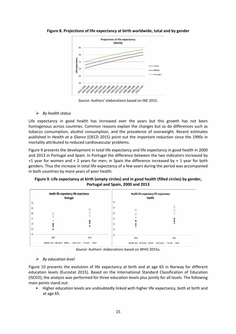
Figure 8 presents the assumptions in the international demographic projections – medium variant. The gender gap in life expectancy at birth is assumed to remain constant at 4.5 years until 2050 and to reduce thereafter until 2100, when the gap reaches 3.8 years (INE 2015).
15
Figure 8. Projections of life expectancy at birth worldwide, total and by gender
Source: Authors’ elaborations based on INE 2015.
By health status
Life expectancy in good health has increased over the years but this growth has not been homogenous across countries. Common reasons explain the changes but so do differences such as tobacco consumption, alcohol consumption, and the prevalence of overweight. Recent estimates published in Health at a Glance (OECD 2015) point out the important reduction since the 1990s in mortality attributed to reduced cardiovascular problems.
Figure 9 presents the development in total life expectancy and life expectancy in good health in 2000 and 2013 in Portugal and Spain. In Portugal the difference between the two indicators increased by +1 year for women and + 2 years for men; in Spain the difference increased by + 1 year for both genders. Thus the increase in total life expectancy of a few years during the period was accompanied in both countries by more years of poor health.
Figure 9. Life expectancy at birth (empty circles) and in good health (filled circles) by gender, Portugal and Spain, 2000 and 2013
Source: Authors’ elaborations based on WHO 2015a.
By education level
Figure 10 presents the evolution of life expectancy at birth and at age 65 in Norway for different education levels (Eurostat 2015). Based on the International Standard Classification of Education (ISCED), the analysis was performed for three education levels plus jointly for all levels. The following main points stand out:
• Higher education levels are undoubtedly linked with higher life expectancy, both at birth and at age 65.

16
• The development over time was neither uniform nor steady. It is not clear whether this represents stochastic variations, cohort specificities, or data issues.
• Comparing data at the end-points of 2007 and 2013, the increase in life expectancy for lower-educated men was higher than that for higher-educated men (1.9 percent compared to 1.2 percent).
• For women, the result was the opposite –those with the highest education level had an increase in life expectancy of 1.1 percent, well above the gain for those with the lowest level of education (0.4 percent).
Figure 10. Life expectancy at birth and at age 65 by education level and gender, Norway, 2007–2013
Source: Authors’ elaborations based on Eurostat 2015.
Figure 11 offers a similar elaboration based not on profession. The analysis was undertaken by the Office for National Statistics (2011) for England and Wales for a longer period, covering the years 1972/76 to 2002/06. The following main points stand out:
• For all professions, life expectancy at birth and at age 65 increased across the investigated period.
• The development over time was neither uniform nor steady. Again, it is not clear whether this represents stochastic variations, cohort specificities, or data issues.
• Those in liberal professions achieved stronger growth in life expectancy at birth, for both men (11.8 percent) and women (7.8 percent), compared to those in more manual professions (9.8 percent for men and 5.5 percent for women).
• A similar but more differentiated picture emerges when changes in life expectancy at age 65 are considered. Those in liberal professions showed stronger growth in life expectancy at age 65, for both men (32.4 percent) and women (14.9 percent), compared to those in more manual professions (25.1 percent for men and 6.8 percent for women).

17
Figure 11. Life expectancy at birth and at age 65 by profession and gender, England and Wales, 1972/76 to 2002/06
Source: Authors’ elaborations based on Office National Statistics 2015.
By income level
Last but not least, Figure 12 offers the evolution of life expectancy at birth and at age 65 in Canada by income quintile for the data points 2000/02 and 2005/07. The following main points stand out:
• Despite the short time interval analyzed, all income quintiles exhibited an increase in life expectancy.
• Men in the highest income quintile experienced an increase in life expectancy at birth of 1.4 percent, while men in the lowest income quintile increased life expectancy by 2 percent.
• For women, the difference between the increase in life expectancy between those in the highest and lowest quintiles was closer, at 1.1 percent and 1.4 percent, respectively.
• For life expectancy at age 65, the relative ranking between highest and lowest income quintile and gender was more pronounced: 6.1 percent versus 7.5 percent for high-and low-income men, respectively, and 3.8 percent versus 4.5 percent for high-and low-income women, respectively.

18
Figure 12. Evolution of life expectancy at birth and at age 65 by income level and gender, Canada, 2000/02 and 2005/07
Source: Authors’ elaborations based on Statistics Canada, Canadian Vital Statistics, Birth and Death Databases, and population estimates.
Table 4 summarizes the observed trends in life expectancy by socioeconomic dimensions.

19
Table 4: Trends in heterogeneity of longevity: Selective examples by socioeconomic criteria and countries
Socioeconomic dimension
Changes in life expectancy
differences in years
Country Period Comments (column 2)
Gendera
constant/constant World 1990–2013 at birth/ at age 60 constant/+1 Europe
-1/+0.1 Spain
2002–2013
at birth/at age 60 -0,5/+0.1 Portugal -1.2/-0.7 Norway -1.5/+0.1 Hungary
Health statusb +1/+2 Portugal
2000–2013
at birth
(women/men) +1/+1 Spain
Educationc
+0.6/-2.5 Norway 2007–2013
at birth
(women/men) +0.1/-0.7 Italy +1.1/+0.6 Sweden
+1.2/+2 Portugal 2010–2013 at birth (women/men)
Labor activityd
+2/+2.1
England/Wales
1972–2006
at birth
(women/men)
Incomee -0.2/-0.4
+7.6/+9.7
Canada
United States
2000/2002 to
2005/2007
Cohorts 1930/1960
at birth (women/men)
at age 50
(women/men)
Note: aChange in difference in life expectancy between women and men along the period. bChange in difference between total life expectancy and healthy life expectancy along the period. cChange in difference in life expectancy between individuals with high and low levels of education along the period. dChange in difference in life expectancy for individuals with liberal profession and unqualified labor jobs along the period. eChange in difference in life expectancy for individuals with high and low levels of income (5th vs 1st quintile) along the period. Source: Authors based on quoted references.
3.2 Prospects for heterogeneity in longevity
To motivate policy actions to contain or neutralize the effects of heterogeneity in longevity, it is not only important to know the current levels and gaps between socioeconomic groups but also to understand past trends to assess future prospects. Projected diminishing gaps would make the issues less important, while increasing gaps would make them even more so. As the prior subsection suggests, there are very limited indications for a past gap reduction. This subsection offers some brief considerations of future prospects with a focus on income and gender as these are the most critical socioeconomic dimensions for pension policy design.
The prospect of heterogeneity by income indicator is guided by two considerations, both of which suggest a further increase. First, income inequality has increased in recent decades and is likely to remain high for some time (OECD 2011; Cingano 2014). As this process takes some time to affect

20
lifetime income and the pension base, lifetime-relevant income inequality is likely to increase. Ceteris paribus, this will increase heterogeneity in longevity. Second, for a given (lifetime) income inequality, the correlation between (lifetime) income and longevity heterogeneity may further increase, at least at the tails of the distribution. The more precarious work conditions in recent decades and higher cyclical and structural unemployment may put downward pressure on both income and longevity for the lowest income groups. On the other hand, the highest period and lifetime income groups are likely to continue profiting from better access to health care, better nutrition decisions, and other life-extending factors.
Regarding the prospects of heterogeneity vis-à-vis gender, past trends and projected societal developments suggest the following: On one hand, the observed mild reduction in the gender gap for most countries in recent decades is likely to continue in coming decades; as a result the gap will shrink but remain sizable and will not disappear in most countries. On the other hand, the gender gap may not follow a smooth decline in some countries but re-increase as the result of socioeconomic shocks, as seen in Russia and other countries during economic transition.
For other socioeconomic indicators, too little information exists to offer informed prospects. We can only formulate two research questions for attention in the years to come: First, what is the scope of the supplementary heterogeneity delta for other relevant socioeconomic dimensions above the income indicator, and is it going to rise due to economic and social developments (such as more heterogeneous societies, greater prevalence of overweight/obesity, environmental challenges, etc.)? Second, what other relevant indicators have been omitted so far in the analyses due to lack of data?
4. Data options and data needs
The prior two sections offer strong indications on the scope of heterogeneity in longevity for a diverse set of socioeconomic indicators and their broad past and possible future trends. The reviewed studies are based on available data typically collected for other purposes; thus the indicators used for the socioeconomic dimensions analyzed are only proxies for the true indicators we would like to measure. Against this background, this section presents three issues for further attention: (i) identifying what relationship between longevity and with what kind income variable we ideally want to establish; (ii) estimating the beyond-income heterogeneity delta for other socioeconomic dimensions; and (iii) proxying income data via other socioeconomic dimensions.
(i) With what income variable do we want to associate longevity heterogeneity?
To establish a wish list of indicators for income and other socioeconomic variables, we go back to our basic concern and objective of analysis: to identify the key distortions created by heterogeneous longevity that risk impacting the functioning of social security programs (particularly pensions) and the effectiveness of key reform options (particularly the move toward DC-type schemes and an increase in retirement age). Such distortions will emerge if the contribution effort or perceived acquired rights are not matched by concomitant pension payouts.
Against such considerations the favored income variables are suggested to be accumulated contributions (AK) under a DC scheme – whether notional or financial – or acquired rights under a defined benefits (DB) scheme (i.e., pension wealth PW) – measured under the relevant population average survival probability – with both AK and PW measured at identical retirement age(s). The relevant heterogeneity indicator for longevity is life expectancy at retirement or, in some considerations, the vector of survival probabilities at retirement.
While empirical data that can establish a statistical link between individuals’ “income” (i.e., actually the wealth variables AK or PW) and their ex-post life expectancies would be great progress in data precision, the complete data arrive only 40 years or more after the income variable has been generated. Such a time lag puts into doubt the operational usefulness of such an approach, albeit it is conceptually useful as analytical benchmark.

21
This calls for approximations in the establishment of the heterogeneity link through other data, such as proxying the cohort approach via cross-section data for survival probabilities/life expectancy or some mixed approaches. Under some considerations, the pension wealth under DB schemes may not be the appropriate indicator to establish the potential distortions of heterogeneity but to calculated hypothetical contribution assets for individuals at retirement (i.e., some measure of contributions actually paid). Last but not least, the question emerges as to the extent to which period income differences in selected broad income measures can be used to proxy differences in lifetime income.
(ii) Establishing the beyond-income heterogeneity delta
For our purposes, establishing the (lifetime) income/longevity heterogeneity link is of fundamental importance as the accumulated amount to be annuitized and the survival probabilities are the basic ingredients for any life annuity contract. As highlighted throughout the prior sections, other socioeconomic dimensions are closely linked with income – as input for longevity or as outcome, such as education and health. But we do not know how much each of these dimensions singly or all together adds to the income effect once we control for income and endogeneity (and differentiate by age, gender, and perhaps even race).
Establishing the heterogeneity delta puts significant demands on the required data and on the estimation approaches. The ideal database would include the joint distribution of survival probabilities across all socioeconomic dimensions considered relevant, at least from the age of retirement onward; for deeper heterogeneity considerations, this would be required from the age of entry into the labor market or even birth. Much less demanding would be data on life expectancy across relevant socioeconomic dimensions, but even such data do not (yet) exist. Consequently, operational approaches must borrow and match data from different countries.
To quantify socioeconomic mortality differentials, alternative methods may be used such as generalized linear models (Madrigal et al. 2011), survival models (Richards 2008), or multiple population extensions of the Lee-Carter model (Lee and Carter 1992), including the use of relational models based on modeling mortality in socioeconomic subpopulations alongside the mortality of a reference population (Li and Lee 2005; Russolillo, Giordano, and Haberman 2011). Some of the associated challenges are presented in Box 1.
(iii) Proxying income data via other socioeconomic dimensions
For many countries, even the data needed to explore heterogeneity by income dimension do not (yet) exist or are not exploited. Social security institutions with complete electronic storage would, in principle, have the database to sort longevity outcomes by contribution accumulations/benefit levels/pension wealth at retirement. If these data are not available or are incomplete, then one needs to find alternatives, such as proxying income data via other socioeconomic dimensions – e.g., education (years of school or highest level achieved), health status, etc. Estimated longevity profiles by socioeconomic indicators from own and similar countries would offer a possible starting position.
5. Implications of longevity heterogeneity for labor market outcomes and pension scheme designs
This section sketches some of the key implications of the heterogeneity in longevity for labor market outcomes and pension system design. A companion paper under preparation elaborates on each of these and other points and presents policy designs to correct for heterogeneity effects.
5.1 The tax-subsidy character of heterogeneous longevity
The first point to make is that heterogeneous life expectancy acts like a tax for some participants in a pension scheme and as a subsidy for others. Compared to the average of participants in a scheme, an individual with a below-average life expectancy receives a lower annuity value for his contributions. This is akin to a tax on his contributions whereby the tax rate is higher the lower his

22
life expectancy relative to the pool’s average. For an individual with an above-average life expectancy, this amounts to a subsidy for his contributions, whereby the subsidy rate is higher the higher his life expectancy above the pool’s average.
The level of the tax or subsidy rate resulting from the life expectancy gap can be easily formalized and calculated under assumptions that are not very restrictive.
Consider individuals who have all accumulated the same savings amount at retirement to be converted into an annuity. Assume they retire at the same age and face the same interest rate, but have different life expectancies.
Let t (s) be the implicit tax (subsidy) rate. AK is the accumulation at retirement, α is the annuity rate, p is the pension, and PW is pension wealth. The subscript i denotes individual values and subscript a the average values of these variables.
The pension for each individual is the annuity rate applied to the identical wealth accumulation:
[1] pi = α.AK
Each individual’s PWi is different from everyone else’s to the extent that his/her life expectancy (LE) differs. PW can be written in this simple form if the interest rate equals the growth rate (indexation) of pensions:
[2] PWi = pi.LEi = α.AK.LEi
With these elements we can easily define the tax (subsidy) rate as the difference in pension wealth compared to the average:
[3a] t(s)i = (a.AK.LEi – a.AK.LEa) / a.K.LEa = LEi/ LEa - 1
Box 1: Some Challenges to Modelling Mortality
The simplest approach for modeling mortality in a set of subpopulations is to use independent, unrelated Lee-Carter models for each subpopulation. The independent modeling approach is straightforward to implement but has several shortcomings. The main one is that it assumes no interdependence among the mortality of subpopulations, a very unrealistic assumption for socioeconomic subpopulations within a country, which are likely to follow similar mortality trends. The assumption of complete independence among subpopulations can be relaxed by using multivariate time series methods. An alternative approach for modeling mortality differentials is the joint time trend model proposed by Lee and Carter (1992).
Many of these statistical methods were specifically proposed to assess baseline (level) mortality differentials, neglecting (to some extent because of lack of appropriate data) differences in improvements by socioeconomic characteristics and the modeling of their possible future evolution. Provided that data requirements are met, an appropriate model should allow for both level and trend differentials in mortality, as well as the projection of their future evolution.
Additional desirable features of an approach for modeling and forecasting mortality in a group of socioeconomic subpopulations include: consistency of subpopulation-specific mortality forecasts with national mortality forecasts; ability to forecast mortality rates that preserve the inverse relationship between socioeconomic circumstances and mortality; transparency for understanding level and improvement differentials in mortality; and the ability to produce interval forecasts of mortality differentials.
23
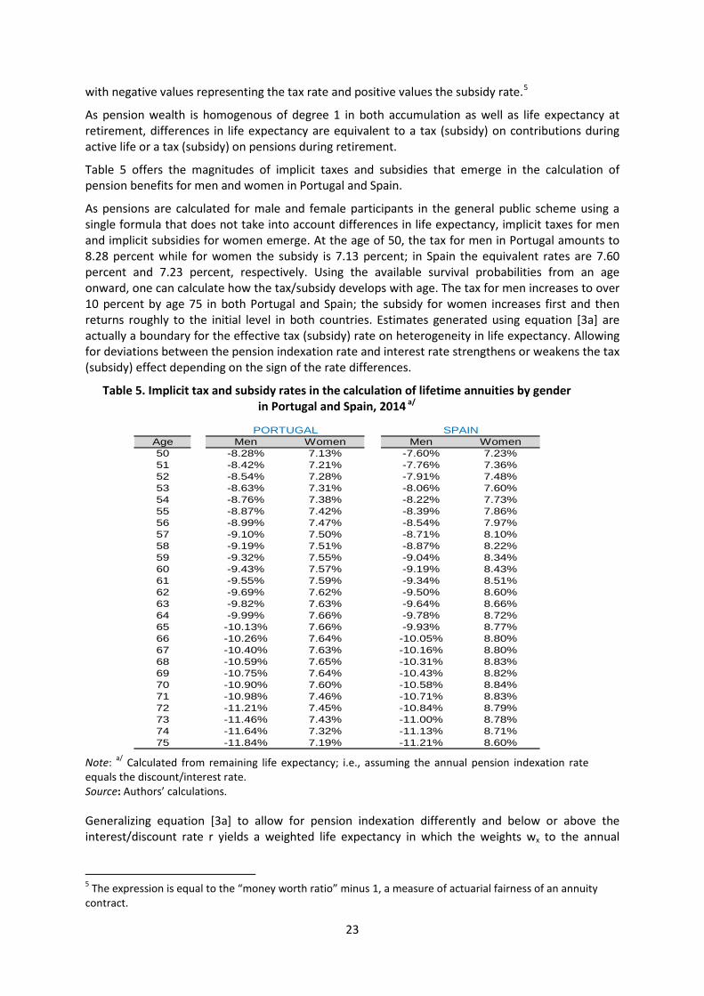
with negative values representing the tax rate and positive values the subsidy rate.5
As pension wealth is homogenous of degree 1 in both accumulation as well as life expectancy at retirement, differences in life expectancy are equivalent to a tax (subsidy) on contributions during active life or a tax (subsidy) on pensions during retirement.
Table 5 offers the magnitudes of implicit taxes and subsidies that emerge in the calculation of pension benefits for men and women in Portugal and Spain.
As pensions are calculated for male and female participants in the general public scheme using a single formula that does not take into account differences in life expectancy, implicit taxes for men and implicit subsidies for women emerge. At the age of 50, the tax for men in Portugal amounts to 8.28 percent while for women the subsidy is 7.13 percent; in Spain the equivalent rates are 7.60 percent and 7.23 percent, respectively. Using the available survival probabilities from an age onward, one can calculate how the tax/subsidy develops with age. The tax for men increases to over 10 percent by age 75 in both Portugal and Spain; the subsidy for women increases first and then returns roughly to the initial level in both countries. Estimates generated using equation [3a] are actually a boundary for the effective tax (subsidy) rate on heterogeneity in life expectancy. Allowing for deviations between the pension indexation rate and interest rate strengthens or weakens the tax (subsidy) effect depending on the sign of the rate differences.
Table 5. Implicit tax and subsidy rates in the calculation of lifetime annuities by gender in Portugal and Spain, 2014 a/
Age Men Women Men Women50 -8.28% 7.13% -7.60% 7.23%51 -8.42% 7.21% -7.76% 7.36%52 -8.54% 7.28% -7.91% 7.48%53 -8.63% 7.31% -8.06% 7.60%54 -8.76% 7.38% -8.22% 7.73%55 -8.87% 7.42% -8.39% 7.86%56 -8.99% 7.47% -8.54% 7.97%57 -9.10% 7.50% -8.71% 8.10%58 -9.19% 7.51% -8.87% 8.22%59 -9.32% 7.55% -9.04% 8.34%60 -9.43% 7.57% -9.19% 8.43%61 -9.55% 7.59% -9.34% 8.51%62 -9.69% 7.62% -9.50% 8.60%63 -9.82% 7.63% -9.64% 8.66%64 -9.99% 7.66% -9.78% 8.72%65 -10.13% 7.66% -9.93% 8.77%66 -10.26% 7.64% -10.05% 8.80%67 -10.40% 7.63% -10.16% 8.80%68 -10.59% 7.65% -10.31% 8.83%69 -10.75% 7.64% -10.43% 8.82%70 -10.90% 7.60% -10.58% 8.84%71 -10.98% 7.46% -10.71% 8.83%72 -11.21% 7.45% -10.84% 8.79%73 -11.46% 7.43% -11.00% 8.78%74 -11.64% 7.32% -11.13% 8.71%75 -11.84% 7.19% -11.21% 8.60%
PORTUGAL SPAIN
Note: a/ Calculated from remaining life expectancy; i.e., assuming the annual pension indexation rate equals the discount/interest rate. Source: Authors’ calculations.
Generalizing equation [3a] to allow for pension indexation differently and below or above the interest/discount rate r yields a weighted life expectancy in which the weights wx to the annual
5 The expression is equal to the “money worth ratio” minus 1, a measure of actuarial fairness of an annuity contract.

24
survival probability px are smaller or larger than 1 and equal to the period product of the ratio of indexation to discount rate [(1+ d)/(1 + r)]t. Thus the revised equation [3b] is:
[3b] 1, 1,
0 0
1,1,00
11
( ) 1 111
R x R x
i i
i R xR x
aa
dp p wrt sd p wpr
tt
t tt t
tt
tttt
− −
+ += =
−−
++==
+ + = − = −
+ +
∑ ∑
∑∑
where R is the maximum retirement span, x the age of the individual, and t the time index for the retirement period.
Table 6 offers numerical values for equation [3b] using the survival probabilities for Spain weighted under alternative combinations of pension indexation and interest rate assumptions. The diagonal values repeat the results from Table 5 and weights of 1; the border values constitute the result of the combination of extreme assumptions for the pension indexation and interest rates. The other values are somewhere in the middle and are left out of the table for focus and clarity.
As expected, if the weights are smaller than 1 (i.e., d < r), the tax rate as well as the subsidy rate decrease with the difference between indexation and interest rate. If the weights are larger than 1 (i.e., d > r), both tax rate and subsidy rate increase. For relevant and perhaps maximum differences for d-r of some 1.5–2 percentage points, the tax/subsidy rate difference is some 12–20 percent across all combinations; i.e., this is the level of under- or overestimation when tax and subsidy rates are calculated based on unweighted survival probabilities (i.e., life expectancy) instead of weighted ones.
Table 6: Implicit tax and subsidy rates in the calculation of lifetime annuities by gender under alternative pension indexation and discount rates in Spain, 2014
Notes: Calculated from weighted remaining life expectancy at age 60. Source: Authors’ calculations.
The lower tax and subsidy rates in the more relevant case of d<r are due to the stronger frontloading in benefit disbursement. This reduces the implicit tax for those with lower life expectancy as they
Male population to population average
0.000 0.005 0.010 0.015 0.020 0.025 0.030 0.040 0.0500.000 -9.2% -9.6% -10.0% -10.5% -10.9% -11.4% -11.9% -12.8% -13.8%0.005 -8.8% -9.2% -13.3%0.010 -8.4% -9.2% -12.8%0.015 -8.0% -9.2% -12.3%0.020 -7.7% -9.2% -11.8%0.025 -7.3% -9.2% -11.3%0.030 -7.0% -9.2% -10.9%0.040 -6.4% -9.2% -10.0%0.050 -5.9% -6.2% -6.5% -6.8% -7.1% -7.4% -7.7% -8.4% -9.2%
Female population to population average0.000 0.005 0.010 0.015 0.020 0.025 0.030 0.040 0.050
0.000 8.4% 8.8% 9.2% 9.6% 10.0% 10.4% 10.8% 11.6% 12.5%0.005 8.1% 8.4% 12.1%0.010 7.7% 8.4% 11.6%0.015 7.4% 8.4% 11.2%0.020 7.1% 8.4% 10.7%0.025 6.8% 8.4% 10.3%0.030 6.5% 8.4% 9.9%0.040 6.0% 8.4% 9.1%0.050 5.5% 5.7% 6.0% 6.2% 6.5% 6.8% 7.1% 7.8% 8.4%
rate
Pension indexation rate
Interest
Interest
rate

25
have relatively larger benefits earlier on while those that have a relatively higher life expectancy have relatively lower benefits at higher ages.
The presented gender differences in life expectancy for Spain and Portugal are relatively small, resulting in tax/subsidy rates of around 10 percent. The literature review in Sections 2 and 3 suggested that differences in life expectancy vis-à-vis other socioeconomic dimensions, in particular education and/or income, may be substantially larger. Using U.S. data from the 2015 study by the National Academies of Science referenced in Section 2 and translating the gaps in life expectancy between the third (assumed to be the pool average) and other income quintiles into tax/subsidy rates for actuarial annuities indeed provides much higher effects.
Table 6: Implicit tax/subsidy rates by lifetime income quintiles in the United States 1/
Male Quintile 1 Quintile 2 Quintile 3 Quintile 4 Quintile 5 Cohort 1930 -5.3 -3.2 0.0 +6.0 +12.8 Cohort 1960 -21.9 -15.3 0.0 +13.2 +16.2 Female Quintile 1 Quintile 2 Quintile 3 Quintile 4 Quintile 5 Cohort 1930 -0.3 -3.1 0.0 +3.1 +11.7 Cohort 1960 -12.7 -8.3 0.0 +2.2 +29.3
Note: 1/ Applies for fully actuarial annuity. – signals a tax, and + a subsidy rate. The estimates assume the pension indexation rate is equal to the discount rate. Source: Authors’ calculations based on data from National Academies of Sciences 2015.
The estimated tax/subsidy rates for both men and women for the outer quintiles are, indeed, very high and dramatically increase between birth cohorts that are only 30 years apart. The tax rates for men reach 21.9 percent and 12.7 percent for women; the highest subsidy rate is for women, at a rate of 29.3 percent, while for men the highest subsidy rate is 16.2 percent.
The equivalent tax/subsidy rates within the U.S. pension (social security) scheme are smaller but unknown. As the pension formula of the mandated scheme is highly progressive, favoring lower over higher income levels, heterogeneity in life expectancy corrects the progressive feature toward neutrality or even progressivity.
Yet regardless of the benefit formula, the underlying tax and subsidy rates of similar or even lower magnitudes are bound to have an effect on individual behavior, particular on labor market decisions, as discussed next.
5.2 The tax/subsidy effect on labor market decisions
The economic effect of the implicit tax/subsidy rate on labor market decisions is equivalent to levying an additional tax on social security contributions or mandated savings rates (or offering a subsidy on these retirement savings). Even a 10 percent tax/subsidy rate will impact labor market decisions, and a much higher rate even more so. We do not know of any study that has empirically explored labor market reactions to these implicit taxes/subsidies. Conceptually the reaction should not be too different – if at all – from explicit taxes and three labor market effects are in the forefront: the effect on the informality decision, the effect on contribution density, and the effect on the retirement decision.
Faced with an explicit or implicit tax, an individual has two main options: evasion or avoidance.
All countries offer to some extent opportunities to (illegally) evade taxes by working in the informal sector. Doing so allows evading the social security contribution and furthermore any personal income tax that is added. The higher the tax rate, the stronger the incentive to work informally. On the other hand, a subsidy on contributions tends to increase formal labor force participation, with

26
countervailing effects emerging from personal income tax implications. These predictions are consistent with the internationally observed lower formal labor market participation of lower-income groups and higher participation for higher-income groups, a tendency that can be strengthened or weakened by other effects, such as liquidity constraints (see, for example, Levy 2008; Ribe, Robalino, and Walker 2013).
Tax avoidance is a legal reaction of individuals against a tax by avoiding actions that lead to the tax liability. In the case of an implicit tax on contributions, one can reduce work effort or not work in areas subject to contribution obligations. For subsidies on contributions, the opposite reaction is to be expected. These predictions are consistent with differences in the contribution density of individuals across the income spectrum; i.e., lower-income groups have a lower contribution effort due to fewer insured hours, days, or months. Again, other effects may strengthen or weaken the tendency.
Last but not least, a tax or subsidy on pension contributions/retirement savings will affect the retirement decision. In the simplest conceptualization, such a tax creates a convex kink in the intertemporal budget constraint for lower-income groups, making them more likely to retire at the earliest retirement age the higher the tax rate. A subsidy creates a concave kink in the intertemporal budget constraint for higher-income groups, reducing their incentives to retire at the earliest possible age. It also incentivizes, however, an earlier retirement age than would otherwise occur, and which is more likely the higher the subsidy rate. As before, other effects may strengthen or weaken such a tendency.
5.3 Implications for pension reform and scheme design
The empirical importance of these and other labor market effects needs to explored but can be conjectured to be sizable. If correct, this would have major implications for pension reform and scheme design that call for actions of substantial reduction or even elimination. This section briefly discusses the implications for the DC reform agenda, the retirement increase agenda, and the annuitization agenda.6
A main reform movement across the world in recent years was the move from DB schemes to DC schemes, be they funded or unfunded, and within DB schemes to undertake parametric reforms that make them more like DC schemes by increasing the contribution-benefit link (see Holzmann 2012; OECD 2015). A strong contribution-benefit link is motivated by lower labor market distortions and higher equity considerations. But if such a link gets broken by heterogeneity in longevity that is closely linked to income level, then the economic and social rationale for such a reform direction is perhaps not eliminated but very much reduced.
Another main reform movement that has only recently gained traction in developed economies is an increase in retirement age to address population aging. More and more countries are linking the standard retirement age to life expectancy in the expectation that individuals will respond by postponing retirement, as earlier retirement is disincentivized by actuarial decrements. However, faced with lower-than-average life expectancy, many low-income individuals may still have an incentive to retire at the earliest possible age (as discussed above), which makes it politically difficult to increase the minimum retirement age while offering those individuals an ever-lower initial pension benefit. But subsidies for higher-income groups risk dampening the envisaged later retirement effects, as the income effect of higher benefits may dominate.
Lastly, another reform movement in recent years was the move from unfunded to funded schemes in some countries, and in many countries a reduction in public generosity expected to be compensated by voluntary individual savings efforts. While the retirement funding volume across
6 For an early analysis of the implications of socioeconomic heterogeneity in mortality on pension reform policy, see Whitehouse and Zaidi (2008).

27
the world has undoubtedly increased in recent decades and years (see Towers Watson 2016), life annuities as a main disbursement form of funded pension provisions received limited attraction or even declined in most countries. Such a trend may have both demand- and supply-side explanations (see Bravo and Holzmann 2014; Holzmann 2015; Reichling and Smetters 2015). For example, heterogeneity in longevity and its increase in recent years may have significantly contributed to this trend (including forced insurance pooling across genders in private annuity contracts in various countries).
6. Conclusions and next steps
The review of data across countries suggests that heterogeneity in longevity by socioeconomic groups is sizable and not likely to decrease in the near future. The available data reveal that heterogeneity measured via mortality rates or life expectancy exists across many socioeconomic characteristics: some are exogenous (such as age, gender, and race), while others are more amenable to individual action (such as health, education, profession, location, and income). All are interlinked and causes and effects are not easily established.
The heterogeneity in life expectancy disaggregated by key socioeconomic characteristics in most countries is stunning. For example in many countries the gender differences in life expectancy at birth are some 5 to 7 years, and still 3 to 4 years at age 60. Differences by education level in some countries may be only a few years for both men and women but reach 15 years (men) and 8.1 years (women) at age 30 in others. These and other longevity gaps show little trend for closure.
The prospects for longevity heterogeneity vis-à-vis income may not improve soon either. Income inequality has increased in recent decades and is likely to remain high in many countries. As this process takes some time to affect lifetime income and the pension base, lifetime-relevant income inequality is likely to increase. Ceteris paribus, this will increase heterogeneity in longevity by income. In addition, for a given (lifetime) income inequality, the correlation between (lifetime) income and longevity heterogeneity may further increase, at least at the tails of the distribution. The more precarious work conditions in recent decades and higher cyclical and structural unemployment may put downward pressure on both income and longevity for the lowest income groups.
As heterogeneity in longevity is closely linked to income (i.e., the contribution base of earnings-related social programs such as pensions), and is empirically sizable, major implicit taxes result for some groups – particularly the less educated and low earners – while offering major subsidies for other groups – particularly highly educated individuals and high-income earners. The implicit tax and subsidy rates on individual contributions are likely to be high, reaching 20 percent and more in many countries, and amounting to up to, perhaps, 50 percent in both directions in some countries.
The implications for such high tax and subsidy rates on pension reform and scheme design are substantial as they counteract the envisaged effects of a closer contribution-benefit link, an increased formal retirement age as a key instrument to address population aging, and more individual funding and private annuities to compensate for reduced public generosity. If unchecked, such high implicit tax and subsidy rates risk also aggravating further informality in countries and sustained low contribution density by lower-income groups, all detrimental to increased pension coverage and equitable pension benefits.
To address heterogeneity in longevity and its link to income, various policy options may be envisaged, acting on the benefit design and revenue distribution side. While a number of complex interventions may be imagined to compensate for heterogeneity, the solution should be simple, operational, and transparent. A companion paper under preparation deepens the empirical analysis on the scope of the implicit tax and subsidy, reviews key policy options, models the most prominent policy option to assess the degree to which heterogeneity effects can be reduced, and offers suggestions on how current reform directions need to and can be adjusted.

28
References
Alaminos, Estefanía, and Mercedes Ayuso. 2015. “Una estimación actuarial del coste individual de las pensiones de jubilación and viudedad: Concurrencia de pensiones del Sistema de la Seguridad Social español.” Estudios de Economía Aplicada 33 (3): 1‐22.
Ayuso, Mercedes, and Montserrat Guillén. 2011. “El coste de los cuidados de larga duración en España bajo criterios actuariales: ¿es sostenible su financiación?”. En El Estado de bienestar en la encrucijada: nuevos retos ante la crisis, Ekonomi Gerizan, Federación de Cajas de Ahorro Vasco‐Navarras: 213‐227.
Ayuso, Mercedes, and Robert Holzmann. 2014. “Longevidad: un breve análisis global y actuarial,” Instituto BBVA de Pensiones – Documento de Trabajo No 1/2014, Septiembre. Madrid: BBVA.
Ayuso, Mercedes, Jorge Bravo, and Robert Holzmann. 2015. “Revisión de las proyecciones de población – Parte 1: Más allá de los convenientes supuestos sobre fertilidad, mortalidad y migración.” Instituto BBVA de Pensiones – Documento de Trabajo No 10/2015, Marzo. Madrid: BBVA.
Bolancé, Catalina, Ramón Alemany, and Montserrat Guillén. 2013. “Sistema público de dependencia y reducción del coste individual de cuidados a lo largo de la vida”. Revista de Economía Aplicada 61: 97‐117.
Borrell, Carmen, et al. 1997. "Widening social inequalities in mortality: the case of Barcelona, a southern European city." Journal of Epidemiology and Community Health 51(6): 659‐667.
Borrell, Carme, et al. 1999. "Inequalities in mortality according to educational level in two large Southern European cities." International Journal of Epidemiology 28(1): 58‐63.
Bravo, Jorge, and Robert Holzmann. 2014. “La fase de percepción de los pagos de los planes de pensiones provisionados: riesgos y opciones de pago.” Documento de Trabajo: Nº 6/2014. Madrid: Instituto BBVA de Pensions.
Brønnum‐Hansen, Henrik, et al. 2004. "Social gradient in life expectancy and health expectancy in Denmark." Sozial‐und Präventivmedizin 49(1): 36‐41.Case, Ann, and Angus Deaton. 2015. “Rising morbidity and mortality in midlife among white non‐Hispanic Americans in the 21st century.” PNAS – Social Sciences September 17.
Castelló‐Climent, Amparo, and Rafael Doménech. 2008. “Human Capital Inequality, Life Expectancy and Economic Growth”. The Economic Journal 118: 653‐677.
Cingano, Federico 2014. “Trends in Income Inequality and its Impact on Economic Growth.” OECD Social, Employment and Migration Working Papers, No. 163. OECD Publishing. http://dx.doi.org/10.1787/5jxrjncwxv6j‐en
Crimmins, Eileen M., Mark D. Hayward, and Yasuhiko Saito. 1994. "Changing mortality and morbidity rates and the health status and life expectancy of the older population." Demography 31(1): 159‐175.
Crimmins, Eileen M., Mark D. Hayward, and Yasuhiko Saito. 1996. "Differentials in active life expectancy in the older population of the United States." The Journals of Gerontology Series B: Psychological Sciences and Social Sciences 51(3): S111‐S120.
Chande, Roberto Ham. 2001. "Esperanzas de vida y expectativas de salud en las edades avanzadas." Estudios demográficos y urbanos 48: 545‐560.
Chang, Man‐Huei, et al. 2015. "Differences in healthy life expectancy for the US population by sex, race/ethnicity and geographic region: 2008." Journal of Public Health 37(3): 470‐479.
Chetty, Raj, Michael Stepner, Sarah Abraham, Shelby Lin, Benjamin Scuderi, Nicholas Turner, Augustin Bergeron, and David Cutler. 2016. “The Association Between Income and Life
29
Expectancy in the United States, 2001‐2014.” Clinical Review & Education. JAMA. doi:10.1001/jama.2016.4226, Published online April 10, 2016.
Deeg, D. J. 2001. “Sex‐Differences in the Evolution of Life Expectancy and Health in Older Age.” In Robin et al. (Eds.) Sex and Longevity: Sexuality, Gender, Reproduction, Parenthood, Book Series Research and Perspectives in Longevity, 129‐140.
Doblhammer, Gabriele, Roland Rau, and Josef Kytir. 2005. "Trends in educational and occupational differentials in all‐cause mortality in Austria between 1981/82 and 1991/92." Wiener Klinische Wochenschrift 117(13‐14): 468‐479.
Dowd, Jennifer B., and Amar Hamoudi. 2014. "Is life expectancy really falling for groups of low socio‐economic status? Lagged selection bias and artefactual trends in mortality." International Journal of Epidemiology 43(4): 983‐988.
Duggan, James E., Robert Gillingham, and John S. Greenlees. 2007. "Mortality and lifetime income: Evidence from Social Security records." Working paper 07/15, International Monetary Fund.
Duleep, Harriet Orcutt. 1989. "Measuring socioeconomic mortality differentials over time." Demography 26(2): 345‐351.
Eurostat. 2015. “Mortality and life expectancy statistics”. Eurostat Statistics Explained.
Geruso, Michael. 2012. "Black‐White Disparities in Life Expectancy: How Much Can the Standard SES Variables Explain?." Demography 49(2): 553‐574.
Gómez‐Redondo, Rosa, and Carl Boe. 2005. "Decomposition analysis of Spanish life expectancy at birth." Demographic Research 13(20): 521‐546.
Herce, José Antonio. 2015. “Las pensiones en las Comunidades Autónomas”. Instituto BBVA de Pensiones – Documento de Trabajo No 12/2015, Marzo. Madrid: BBVA.
Holzmann, Robert. 2012. “Global pension systems and their reform: Worldwide drivers, trends and challenges.” International Social Security Review 66(2).
Holzmann, Robert. 2013. “A Optimistic Perspective on Population Aging and Old‐Age Financial Protection.” Malaysian Journal of Economic Studies 2013 50(2): 107‐137. Updated and
revised Chinese translation in 劳动经济研究 (Studies in Labor Economics 2(4): 2014: 21‐52, Chinese Academy of Social Science).
Holzmann, Robert. 2015. “Addressing Longevity Risk Through Private Annuities: Issues and Options.” Conference paper presented at the 13th International Workshop on Pension Insurance and Savings Paris Dauphine, 28 May.
INE (Instituto Nacional de Estadística). 2015. Discapacidad (tasas, esperanzas de vida en salud). Madrid.
Judge, Ken. 1995. "Income distribution and life expectancy: a critical appraisal." British Medical Journal 311(7015): 1282.
Kalwij, Adriaan S., Rob J.M. Alessie, and Marike G. Knoef. 2013. "The association between individual income and remaining life expectancy at the age of 65 in the Netherlands." Demography 50(1): 181‐206.
Kaplan, Robert M., and Michael L. Spittel, and Tia L. Zeno. 2014. "Educational Attainment and Life Expectancy." Policy Insights from the Behavioral and Brain Sciences 1(1): 189‐194.
Kaplan, Robert M., and Richard G. Kronick. 2006. “ Marital status and longevity in the United States population.” Journal of Epidemiology and Community Health 60(9): 760‐765.
Lee, R.D., and L.R. Carter. 1992. “Modeling and Forecasting U.S. Mortality.” Journal of the American Statistical Association 87: 659–671.
Levy, Santiago. 2008. Good Intentions, Bad Outcomes. Washington, DC: Brookings Institution.
Li, N., and R. Lee. 2005. “Coherent Mortality Forecasts for a Group of Populations: An Extension of the Lee‐Carter Method.” Demography 42: 575–594.

30
Lin, Charles C., et al. 2002. "A further study of life expectancy by socioeconomic factors in the National Longitudinal Mortality Study." Ethnicity & disease 13(2): 240‐247.
Lleras‐Muney, Adriana. 2005. "The relationship between education and adult mortality in the United States." The Review of Economic Studies 72(1): 189‐221.
Madrigal, A., F. Matthews, D. Patel, A. Gaches, and S. Baxter. 2011. “What Longevity Predictors Should be Allowed for When Valuing Pension Scheme Liabilities.” British Actuarial Journal 16: 1–38.
Meara, Ellen R., Seth Richards, and David M. Cutler. 2008. "The gap gets bigger: changes in mortality and life expectancy, by education, 1981–2000." Health Affairs 27(2): 350‐360.
Miech, Richard, et al. 2011. "The enduring association between education and mortality the role of widening and narrowing disparities." American Sociological Review 76(6): 913‐934.
Monteverde, Malena. 2004. “Discapacidades de las personas mayores en España: prevalencias, duraciones e impacto sobre los cuidados de larga duración”. Tesis doctoral. Universitat de Barcelona.
National Academies of Sciences, Engineering, and Medicine. (2015). “The Growing Gap in Life Expectancy by Income: Implications for Federal Programs and Policy Responses.” Committee on the Long‐Run Macroeconomic Effects of the Aging U.S. Population‐Phase II. Committee on Population, Division of Behavioral and Social Sciences and Education. Board on Mathematical Sciences and Their Applications, Division on Engineering and Physical Sciences. Washington, DC: The National Academies Press.
Office National Statistics. 2011. “Trends in life expectancy by National Statistics Socio‐economic Classification, 1982‐2006, England and Wales.” Statistical Bulletin. Newport.
______2015. “Trend in life expectancy at birth and at age 65 by socio‐economic position based on the National Statistics Socio‐economic Classification, England and Wales: 1982—1986 to 2007—2011.” Statistical Bulletin. Newport.
OECD. 2011. Divided We Stand: Why Inequality Keeps Rising. Paris: OECD.
OECD. 2014. Health at a glance. Europe 2014. Joint publication of the OECD and the European Commission. Paris: OECD.
OECD. 2015. Health Statistics 2015. Paris: OECD.
OECD. 2016. “Fragmentation of retirement markets due to differences in life expectancy”, in OECD Business and Finance Outlook 2016, OECD Publishing, Paris: 177‐205.
Oeppen, Jim, and James V. Vaupel. 2006. “The Linear Rise in the Number of Our Days”. In Bengtsson and Palmer (Eds.) Perspectives on mortality forecasting, Social Insurance Studies, 3. Stockholm: Swedish Social Insurance Agency.
Olshansky, S. Jay, et al. 2012. "Differences in life expectancy due to race and educational differences are widening, and many may not catch up." Health Affairs 31(8): 1803‐1813.
Pijoan‐Mas, Josep, and José‐Víctor Ríos‐Rull. 2014. "Heterogeneity in expected longevities." Demography 51(6): 2075‐2102.
Reichling, Felix, and Kent Smetters. 2015. “Optimal Annuitization with Stochastic Mortality and Correlated Medical Costs.” American Economic Review 105(11): 3273‐3320.
Rendall, M.S, M.M. Weden, M.M. Favreault, and H. Waldron. 2011. “The protective effect of marriage for survival: a review and update.” Demography 48(2): 481‐506.
Ribe, Helena, David Robalino, and Ian Walker. 2012. “From Right to Reality: Incentives, Labor Markets, and the Challenge of Achieving Universal Social Protection in Latin America and the Caribbean.” Latin American Development Forum Series. Washington, DC: World Bank.
Richards, S. 2008. “Applying Survival Models to Pensioner Mortality Data.” British Actuarial Journal 14: 257–303.

31
Russolillo, M., G. Giordano, and S. Haberman. 2011. “Extending the Lee‐Carter Model: A Three‐Way Decomposition.” Scandinavian Actuarial Journal 2: 96–117.
Singh, Gopal K., and Mohammad Siahpush. 2006. "Widening socioeconomic inequalities in US life expectancy, 1980–2000." International Journal of Epidemiology 35(4): 969‐979.
Solé‐Auró, Aïda, Hiram Beltrán‐Sánchez, and Eileen M. Crimmins. 2015. "Are Differences in Disability‐Free Life Expectancy by Gender, Race, and Education Widening at Older Ages?." Population Research and Policy Review 34(1): 1‐18.
Steingrímsdóttir, Ólöf Anna, et al. 2012. "Trends in life expectancy by education in Norway 1961–2009." European Journal of Epidemiology 27(3): 163‐171.
Towers Watson. 2016. Global Pension Assets Study 2016. https://www.willistowerswatson.com
United Nations. 2013. World Mortality Report 2013. Department of Economic and Social Affairs ‐ Population Division, New York.
United Nations. 2015. World Mortality Wallchart 2015. Department of Economic and Social Affairs ‐ Population Division, New York.
Von Gaudecker, Hans Martin, and Rembrandt Scholz. 2007. "Differential mortality by lifetime earnings in Germany." Demographic Research 17(4): 83‐108.
Wikipedia. 2016. Demographics in Russia.
Whitehouse, Edward, and Ashgar Zaidi. 2008. “Socio‐Economic Differences in Mortality: Implications for Pensions Policy.” OECD Social, Employment and Migration Working Papers, No. 71. OECD Publishing. http://dx.doi.org/10.1787/231747416062
World Health Organization (WHO). 2015a. World health statistics 2015. Geneva: WHO.
World Health Organization (WHO). 2015b. World report on ageing and health. Geneva: WHO.