on the linkage between financial risk tolerance and risk - gate
TRANSCRIPT

On the Linkage between Financial Risk Tolerance and Risk Aversion: Evidence from a Psychometrically-validated Survey
versus an Online Lottery Choice Experiment
Robert Faff*
Daniel Mulino
Daniel Chai
Monash University
Abstract In this paper, we explore the linkage between two related concepts describing an individual’s attitude towards risk, namely, financial risk tolerance (FRT) and risk aversion. The former is measured from survey data and the latter from data from lottery experiments. Specifically, we follow a two stage process: (1) we obtain FRT scores from a psychometrically-validated survey on a sample of 162 people; and (2) we conduct a battery of lottery choice experiments on the same people. The second stage is primarily distinguished from earlier lottery choice experiments by being online and involving non-student subjects. Moreover, we contrast: real and hypothetical payoffs; low and high stake payoffs; decisions involving gains and losses; and order effects. Our key finding is that the two approaches to analysing decision-making under uncertainty are strongly aligned. We present evidence that this is particularly the case for the female participants in our sample. There is also some evidence that the alignment is strengthened when high stake gambles are employed. JEL Classification: D81; G19 Keywords: Financial Risk Tolerance; Risk Aversion; Psychometric Survey; Online Lottery Choice Experiment Acknowledgments: The authors would like to thank FinaMetrica Limited for providing access to their database and Geoff Davey, CEO for information on the operation of their risk profiling system. Thanks are also extended to Vanguard Australia and particularly to Robin Bowerman for his continuing support of this project. We also thank Nicki Chua for her assistance in setting up the experiment. We are extremely grateful for the encouragement of the former JFR Editor, Ted Moore, and for the comments and insights of an anonymous referee, Karen Benson, Philip Brown, Paul De Lange, Robert Durand, Paul Gerrans, Phil Gray, Terry Hallahan, Glenn Harrison, Rob Hudson, Chris Lambert, Mike McKenzie, Andy Marshall, Rick Newby, Barry Oliver, Vanitha Ragunathan and Richard Scheelings and also to seminar participants at Monash University, RMIT and the University of Western Australia. The financial assistance provided by an ARC Linkage grant (LP0560992), together with faculty and departmental support is also gratefully acknowledged. *Corresponding author. Department of Accounting and Finance, Faculty of Business and Economics, Monash University, Victoria, 3800, Australia. Phone: +61 3 9905 2387; Fax: +61 3 9905 2339 email: [email protected]

2
On the Linkage between Financial Risk Tolerance and Risk Aversion: Evidence from a Psychometrically-validated Survey
versus an Online Lottery Choice Experiment
Abstract In this paper, we explore the linkage between two related concepts describing an individual’s attitude towards risk, namely, financial risk tolerance (FRT) and risk aversion. The former is measured from survey data and the latter from data from lottery experiments. Specifically, we follow a two stage process: (1) we obtain FRT scores from a psychometrically-validated survey on a sample of 162 people; and (2) we conduct a battery of lottery choice experiments on the same people. The second stage is primarily distinguished from earlier lottery choice experiments by being online and involving non-student subjects. Moreover, we contrast: real and hypothetical payoffs; low and high stake payoffs; decisions involving gains and losses; and order effects. Our key finding is that the two approaches to analysing decision-making under uncertainty are strongly aligned. We present evidence that this is particularly the case for the female participants in our sample. There is also some evidence that the alignment is strengthened when high stake gambles are employed.

1
I. Introduction
In this paper we bridge two literatures on the attitude to economic/financial risk: financial risk
tolerance (FRT) and risk aversion (RA); in an attempt to see how well they
complement/reinforce each other. Integration of FRT and RA has never been done before and
it offers the realistic prospect of unique insights into both literatures.1 FRT refers to an
investor’s attitude towards risk – the amount of uncertainty or investment return volatility that
an investor is willing to accept when making a financial decision (Grable, 2000). In concept,
FRT is inversely related to the economists’ notion of risk aversion. That is, individuals who
are more (less) risk averse will have a lower (higher) tolerance for financial risk.
In the extant literature, there are three methods for measuring FRT/RA: observing
actual investment behavior, assessing choices in an experimental setting, and creating scores
from survey questionnaires. For example, Schooley and Worden (1996) infer RA from
portfolio allocations and Cohen and Einav (2005) structurally estimate risk aversion using car
insurance data. There is also a growing body of literature that analyses contestant behaviors
on gameshows.2 In assessing choices in an experimental setting, researchers consider either
hypothetical scenarios or where decisions have financial consequences (see, for example,
Barsky et al., 1997; Holt and Laury, 2002 and 2005; Harrison et al., 2005). Finally,
researchers such as Grable and Lytton (1999) and Hallahan et al. (2004) investigate
demographic patterns in FRT scores.
1 We are extremely grateful to an anonymous referee for suggesting this unique focus. 2 Of very recent times there has been considerable activity focusing on the show, Deal or No Deal, which has numerous franchises worldwide. See, for example, Andersen et al. (2006b, c and d), Bombardini and Trebbi (2005); Blavatskyy and Pogrebna (2006a and b); de Roos and Serafidis (2006); Post et al. (2006); and Mulino et al. (2006).

2
With regard to the FRT literature, there is considerable interest in the demographic
‘determinants’ and attention is particularly focused on age, gender, education, income/wealth
and marital status.3 Specifically, while debate still remains on some issues, a range of
common findings are generally observed. First, FRT decreases with age (see, for example,
McInish, 1982; Morin and Suarez, 1983; and Palsson, 1996). Second, females have a lower
preference for risk than males (see, for example, Palsson, 1996; Jianakoplos and Bernasek,
1998; Powell and Ansic, 1997; and Grable, 2000).4 Third, FRT increases with education (see,
for example, Haliassos and Bertaut, 1995). Fourth, FRT increases with income and wealth
(see, for example, Friedman, 1974; Cohn et al., 1975; Shaw, 1996; and Bernheim et al.,
2001). Fifth, single (i.e. unmarried) investors are more risk tolerant (see, for example,
Roszkowski, et al., 1993).
Recently, Holt and Laury (2002) investigate RA in the context of lottery choice
decisions. Specifically, they address the “incentive effects” issue by having their experimental
group of subjects (students) engage in both hypothetical and real lottery games.5 They
examine the effects of payoff magnitudes in an experiment where people have to choose
between a range of matched pairs of ‘safe’ and ‘risky’ gambles.6 Holt and Laury find that the
size of the payoff matters, with RA increasing as the stakes involved grow. They also find that
people exhibit higher levels of risk aversion in hypothetical choices as compared to choices
involving real monetary stakes. A key implication is that “... contrary to Kahneman and
Tversky’s supposition, subjects facing hypothetical choices cannot imagine how they would
actually behave under high-incentive conditions” (Holt and Laury, 2002, p. 1654).
3 Surveys of this literature are available in Grable and Lytton (1998) and Grable and Joo (1999). 4 Other recent studies with a gender focus in the financial markets setting include Atkinson et al. (2003) and Barber and Odean (2001). 5 That is, with “real” games, the subjects receive actual (rather than hypothetical) monetary payoffs. 6 In the smallest base case, ‘1x’, the safe (risky) lottery game’s payoffs are $2 and $1.60 ($3.85 and $0.10), with varying probabilities. In the largest lottery game, ‘90x’, the safe (risky) payoffs are $180 and $144 ($346.50 and $9). ‘90x’ refers to the same lottery experiment except that all payoffs are scaled up by 90 times the base game.

3
As outlined above, there are two related literatures (FRT and RA), that hitherto have
not been compared before, thus providing us an opportunity for a unique methodological
contribution to the literature. The primary goal of our paper is to perform such integration.
Specifically, we select a group of experimental subjects who follow a two stage process. In
the first stage, they complete a full psychometrically-based FRT survey which produces a risk
tolerance score for each individual. Then in the second stage, they play a range of lottery
choice games with both hypothetical and real payoffs (modeled on the Holt and Laury, 2002,
design).
Our experimental setup produces a range of key elements relative to the existing
literature. First, our analysis gives important insights into whether and to what extent the FRT
and risk aversion approaches are compatible. Second, compared to Holt and Laury we have
higher stakes and engage more subjects into such games. Third, we include some rounds of
play in which negative outcomes (‘loss making’) occur, thereby allowing us to draw some
inferences regarding loss aversion and prospect theory.7 Fourth, unlike many other similar
studies we do not use students as subjects. This has the major advantage of giving a more
representative sample of society, including a broader range of education levels, age and
wealth. A final feature is that we implement our lottery experiment using an online web-based
delivery.
Our major findings are easily summarized as follows. Our central result is that
obtaining a financial risk tolerance score from a psychometrically-validated survey versus the
risk aversion type of information deduced from lottery choice experiments are indeed strongly
correlated. Our evidence suggests that this is particularly the case for females. There is also
some suggestion that the FRT-RA linkage is strengthened when high stake gambles are
employed.
7 See Laury and Holt (2005) who find a difference in risk attitudes between losses and gains.

4
II. Research Design and Implementation
There are two key elements to our basic research design. First, all subjects completed a full
psychometrically-validated FRT survey which produced a risk tolerance score for each of
them. Second, all subjects play a range of lottery choice games with both hypothetical and
real payoffs. Details of each element and how they relate to each other are presented in the
following sections.
FRT Survey Element
The use of subjective survey questionnaires is a widely accepted method for assessing FRT.
Because of the complexity of the attitudinal construct, a sophisticated psychological testing
instrument is required (Callan and Johnson, 2003). A good attitudinal test will meet accepted
psychological standards for both face validity (perceived relevance of the questions) and
predictive validity (prediction of later performance or behavior). It will also have reliability
(consistency in results for repeated tests of the same person), as well as having appropriate
test norms so that subjects’ test scores can be interpreted against an appropriate reference
group. FinaMetrica Ltd is an Australian company which uses such an approach to measure
the preferred level of risk of an individual. The FinaMetrica Personal Financial Profiling
system is a proprietary, commercial FRT metric.8 It is a psychometrically-validated attitude
test comprising 25 questions that generate a standardized FRT score (1 to 100),9 in which a
higher score indicates higher risk tolerance.10 It has been available commercially to the
Australian financial planning industry since 1998 and was introduced in the United States in
8 See www.FinaMetrica.com.au for further information about the FinaMetrica system. 9 The scale is normally distributed with a mean of 50 and a standard deviation of 10. 10 The metric has been subject to usability, reliability and norming trials by the University of NSW, exceeding international psychometric standards (web site: http://www.risk-profiling.com/).

5
2002. It can be completed in hard-copy form or accessed through the Internet. Our project
utilizes a database of these FRT scores and associated demographic data.11
We contacted FinaMetrica in early 2005 seeking their assistance in obtaining a sample
of subjects for our experiment. FinaMetrica initially identified a pool exceeding 1000 people
who had recently completed their FRT survey (and also a range of demographic questions).12
From this group, a subset of approximately 600 participants had answered ‘yes’ to a question
administered with the original survey asking whether they would be willing to participate in
follow up surveys relating to financial risk tolerance and attitudes to investing. Our contact at
FinaMetrica kindly agreed to email these 600 people asking if they would be specifically
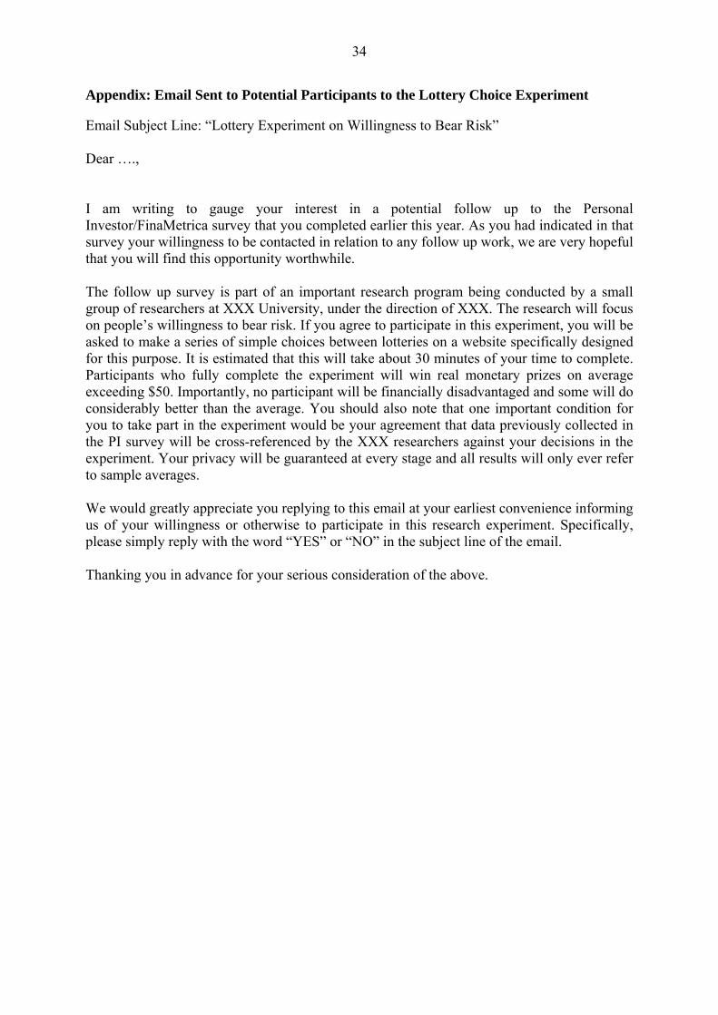
interested in taking part in our experiment (see the Appendix for a transcript of the email
communication). From this group, 250 individuals indicated that they would be willing to
participate and, thus, this subset became the target for our stage 2 lottery experiment.
Lottery Choice Experiment
From the potential pool of 250, 162 people completed the lottery experiment. The big
advantage of this sample compared to many other studies is that we do not rely on students.
The participants in our experiment represent a much broader spectrum of society in many
dimensions including age; wealth; and life experience.13 The setup for this experiment is
explained below.
11 Accompanying the risk tolerance test is a set of eight demographic questions dealing with age, gender, postcode (zipcode), education, income, marital status, financial dependents and net assets. 12 It should be noted that we followed a very lengthy process to obtain full and proper ethical clearance for our project from the ethics committee at our university. As part of that process we agreed to fully respect the confidentiality of all participants. 13 Holt and Laury’s (2002) sample of 175 subjects is made up of (a) undergraduates; (b) MBA students and (c) business school faculty.

6
While we apply Holt and Laury’s (2002) basic lottery choice design, in contrast to
them we create a completely web-based online experiment.14 This has advantages and
disadvantages.15 The experiment comprises a series of “rounds”, with each round involving
10 choices between separate pair-wise lotteries. An example of an illustrative round is
presented in Figure 1 as a “computer screen” view in the web-based format that confronts the
participants. As shown in the figure, Option A represents the safer gamble with a high payoff
of $60 and a low payoff of $48,16 whereas Option B represents the riskier gamble with a high
payoff of $115.50 and a low payoff of $3. Decision 1 in this case, gives a 10% (90%) chance
of the high (low) payoff. For each successive increment down the list, the chance of the high
(low) payoff increases (decreases) by 10% until Decision 10 is reached in which case the high
payoff is fully certain.
After the participant has recorded their choices for a complete round of 10 decisions,
that particular round is completed and the lottery choice program moves on to ascertain the
“outcome” for that participant. The outcome for each round (revealed to each player at the
end of each round prior to starting the next round) is determined by a two stage process. In
step 1 a notional 10-sided die is rolled and the number “revealed” identifies which decision is
“alive”. For example, if the electronic die roll reveals a ‘7’ then it is Decision 7 which is
“alive”. Step 2 involves a second roll of the notional die and the number which comes up
identifies whether a high or low win has occurred. For example, if the second die roll for
14 Full details of how we implement the online experiment are suppressed to conserve space. Suffice it to say, a number of difficulties were encountered and resolved. For example, we needed to design the experiment such that participants could not “cheat”. As a result, two important features were that unique IDs were assigned to each player (password protected) and second we ensured that a real time permanent record of each completed round was made in the database such that a participant could not try and replay a round in the hope of being luckier and winning a larger prize. Holt and Laury (2005) used a computer interface (unlike Holt and Laury, 2002), however, the researcher was present during the experiment and conducted the dice throw by hand. 15 One disadvantage of running the experiment in an online format via email is that a number of participants queried whether the experiment was an internet “scam”. Indeed, one participant contacted an official of our university (independent of our project) to report us as possibly running some scamming operation “legitimized” under the university’s “banner”. 16 All amounts are paid in Australian dollars. At the time of the experiment, the exchange rate was approximately, AU$1 = US$0.75.

7
Decision 7 comes up a ‘2’ (‘9’), then the participant has won either $60 ($48) if they had
chosen Option A or $115.50 ($3) if they had chosen Option B.
Each participant plays between three and six rounds depending on the scenarios
encountered, which will be explained shortly. We designed rounds to vary along a range of
dimensions. First, is stakes – there is a “low” and a “high” case scenario. In the low case
scenario winnings range between $0.10 and $3.85, while the high case scenario winnings
range between $3 and $577.50. Second, is real versus hypothetical rounds. Each round is
clearly designated as being either “real” (and therefore impacting actual money that the
participant will receive) or “hypothetical” (which has no bearing on actual winnings). Third,
is gain versus loss rounds. A gain round involves choice between two positive payoffs,
whereas a loss round involves choice between two negative payoffs.17
There is a maximum of 6 rounds that any participant can play and we list the sequence
of such rounds in Panel A of Table 1. Round 1 is a low payoff (‘1x’), gain and real round.
Rounds 2-5 are high payoff: 2-3 are Gain rounds, while 4-5 are Loss rounds (both are
hypothetical/real pairs). The final round (Round 6) reverts back to the identical scenario of
Round 1. Panel B of Table 1 shows the payoff schedule for the two low rounds (Rounds 1 and
6). The risky (safe) option produces a “good” outcome of $3.85 ($2) and a “bad” outcome of
$0.10 ($1.60).
The reality of running experiments such as ours is the existence of a binding
(relatively low) budget constraint and the challenge is to balance the myriad of competing
issues to arrive at what is seen as the optimal research design. With this in mind, we decided
to “stream” participants into three different high payoff rounds. The highest payoff we were
able to justify was $577.50, but due to budget constraints we couldn’t allow this to be
17 Thus, if it is a real loss round the participants’ actual winnings will necessarily decline. We designed the experiment so that every participant completes it with positive winnings – no one can lose money. We assure participants of this fact prior to them playing the lottery game (see the Appendix).

8
available to any more than about 40 players. Panel C of Table 1 outlines the three streams that
we use. For the gain rounds, Stream 1 corresponds to a ‘30x’ game; Stream 2 a ‘78x’ game
and Stream 3 a ‘150x’ game. As revealed in this table, we need to ensure that the high loss
rounds (Rounds 4 and 5) appropriately “matched” their high gain round counterparts so that
the possibility of “bankruptcy” is eliminated. Indeed, participants who won the lowest amount
in Round 3 automatically bypass Rounds 4 and 5 – they are instead directed straight through
to Round 6.18 We summarize the four possible sequences of play in Panel D of Table 1 – note
that 3 (6) rounds are the minimum (maximum) played.
The potential confounding of “order effects” is an issue that receives some attention in
the literature (see, for example, Harrison et al., 2005 and Holt and Laury, 2005). As Harrison
et al. (2005, p. 897) states, an “ … order effect occurs when prior experience with one task
affects behavior in a subsequent task.” We implement two forms of control to counter-balance
order effects in our experiment. One half of the participants start in Round 1 (with a real, low
payoff scenario), while the others skip Round 1 and start in Round 2 (with an hypothetical,
high payoff scenario). We also ensure that one half of the participants are presented with
“Option A” as the risky option, while the other half are presented with “Option B” as the risky
option (“Option A” is always listed first).
III. Discussion of Experimental Issues
Harrison and List (2004) propose a taxonomy of experiments that includes: conventional lab
experiments; artefactual lab experiments; framed field experiments; and natural field
experiments. Artefactual field experiments differ from conventional lab experiments in that
18 As shown in Panel B of Table 1, the lowest amounts won in Round 3 are $3 (Stream 1); $7.80 (Stream 2) and $15 (Stream 3). The second lowest amounts won in Round 3 are $48; $125 and $240, respectively; which are just able to cover the counterpart maximum losses in Round 5 of -$46.20; -$123 and -$231, respectively.

9
they use a non-standard subject pool. A framed field experiment is an artefactual experiment
with a field context in either the commodity task or information set that contestants can use.
Finally, a natural field experiment is the same as a framed field experiment except the
environment is one where subjects naturally undertake the tasks that are the subject of the
experiment and the subjects do not know that they are in an experiment.
In terms of the parameters of the taxonomy set out above, our experiment differs from
a traditional lab experiment in two important respects. First, we use non-students. According
to Harrison and List (2004), this would be a sufficient innovation to move it into the
“artefactual field experiment” category. Second, our experiment is conducted online. While
still an artificial environment in some respects, it reflects a setting in which many people
regularly undertake commercial transactions today. This is likely to be true for at least some
of the people in our sample, who are informed about the experiment and volunteer for it
online. Our experiment would not fall within the definition of a “natural field experiment” as
set out by Harrison and List, since our participants are aware that they are taking part in an
experiment, but it is nonetheless important to note that the environment in which they make
their decisions is not the same as a conventional lab experiment.
Artefactual Field Experiments
Laboratory experiments in economics are often criticized for relying almost exclusively on
students as subjects. One of the key issues in this debate is whether students are somehow
unrepresentative of the broader population – or rather, whether they are representative, but
simply exhibit less variance in certain demographic characteristics such as age and income. If
the latter is true, then it may be possible (though likely quite difficult) to extrapolate from

10
findings about students by using whatever variance exists.19 If the former is true, then it may
be necessary to take account of selection bias in some other fashion.
Potential Selection Bias
Selection bias could arise in at least two ways. First, people might self-select into being a
student. This could be observed via a comparison of relevant demographic traits across the
overall population and the student population. A second bias might arise in the recruitment
process in terms of the types of students who are most likely to respond to the advertisements
and announcements that induce people to take part in experiments. Some field experiments
avoid the second type of bias (for example, “natural experiments”). In such instances, the only
bias will be via selection into the group that is being studied in its natural environment. One
example of such an experiment is undertaken by Camerer (1998), who studies bookmakers in
their natural environment.
Our experiment, even though arguably conducted in a field setting, certainly has both
biases. Our participants self-select into the pool from which we draw our sample by becoming
connected in some way with FinaMetrica. Among other things, one would expect them to be
wealthier, better educated, more interested in wealth creation and more knowledgeable about
financial transactions than the average person. Participants in our experiment, like student
participants in conventional laboratory experiments, also self-select via the volunteering
process. As in conventional laboratory experiments, we do not correct for this potential bias.
As Harrison and List (2004, p. 1017) note, “… some field experiments face a more
serious problem of sample selection that depends on the nature of the task. Once the
experiment has begun, it is not as easy as it is in the lab to control information flow about the
19 See, for example, Andersen et al. (2006a) who find that the lack of heterogeneity in the student population along some demographic dimensions makes it difficult to estimate the preference heterogeneity that could be present in a more representative sample.

11
nature of the task. This is obviously a matter of degree, but can lead to endogenous subject
attrition from the experiment.” Since our experiment is conducted online, we find it difficult
to control the information flow and, as a result, we have to rely upon highly detailed
instructions to make sure that we cover off on the most likely areas of confusion. However,
we are fortunate in that there is almost no attrition in our experiment. Of those who
volunteered to take part and emailed us requesting a login identity, all but a very small
number fully completed the experiment.
A final issue in relation to selection bias runs in somewhat the opposite direction.
Specifically, certain tasks in the real world may be performed by a very narrow set of people,
making it difficult to extrapolate how such people will behave based on people randomly
chosen for an experiment.20 For example, there may be certain tasks which are subject to
extreme self-selection in the real world, such as risk-loving people being attracted to become
traders. This may be reinforced as people without the necessary aptitude and/or preferences
are subjected to attrition over time. Moreover, people involved in certain real world tasks may
develop skills and behavioral characteristics over time via experience: a process that is usually
very difficult to replicate in time-constrained experiments. These are important considerations
when extrapolating from an experiment to the broader world. However, we believe that the
tasks being performed in this experiment are sufficiently generic and straightforward that this
type of bias should not be a problem.
Are Students Different?
Many studies contrast student samples with non-student samples. For example, Harrison and
Lesley (1996) explore whether it is possible to obtain similar results in a survey of students at
20 For a discussion of the large literature dealing with the role of experience and endogenous institutional design in relation to behavioral defects, see Harrison (2005), Levitt and List (2006, especially pp. 33-38) and Botelho et al. (2007).

12
the University of South Carolina to those collected using a major national survey. They find
that the student survey, when re-weighted to reflect the U.S. population, produces very
accurate estimates of damage valuations. This study suggests that it is limited variance in the
demographic characteristics of students (which can usually be corrected for, at least to some
degree), rather than something inherent in the nature of students per se, that makes students
different from the overall population.21
Nature of the Task
Another important question is whether the nature of the task is too abstract or lacking in field
references for the subjects to fully comprehend what is being asked of them.22 This could be
particularly problematic in our setting given that the experiment is run online and there is
relatively little opportunity for contestants to ask questions.23 However, the nature of our
experiment is such that we are confident that people have adequate reference points: or “field
referents”. The instructions are very detailed and included a number of trial runs. In particular,
it is worth noting that the choices that people make are over dollars, rather than an abstract
unit of measurement such as tickets or points. Moreover, we attempt to make the
randomization process as transparent as possible and use examples and trials before the
experiment proper, to increase subjects’ understanding.
Size of the Stakes
Many argue that the behavior of participants in laboratory experiments involving small stakes
may not reflect their behavior in real world situations involving much higher stakes. One
21 A number of other studies examine non-students. For example, Haigh and List (2005) and Alevy et al. (2007) focus on professional CBOT traders, while Harrison et al. (2005 and 2006) analyze a representative sample of Danish people. 22 Dyer and Kagel (1996) touch on this issue and find that a rule of thumb used by executives in the commercial construction industry to avoid the winners’ curse does not translate to the laboratory. 23 Subjects in our experimental setting could submit queries via email – and in some cases they did so.

13
response to this criticism has been to raise the dollar value of the stakes. Examples include,
Holt and Laury (2002); List and Cherry (2005); and Carpenter et al (2005). This is the
approach that we adopt.24
Hypothetical Stakes
A large experimental literature exists demonstrating that there are differences in the decisions
which people make when there are real financial consequences as opposed to decisions of a
hypothetical nature.25 Holt and Laury (2002) find that subjects in a lottery choice experiment
display lower levels of risk aversion where the choices are hypothetical, as opposed to choices
with real monetary consequences. Similarly, Cameron (1999) finds that Proposer behavior
displays greater variance and Responders are significantly more likely to reject offers when
games involved hypothetical stakes. Our experiment contrasts lottery choices with both real
and hypothetical stakes, broadly supporting the findings of these earlier studies.
The Environment of the Field Study
Most laboratory experiments seek to create an environment that controls for all external
stimuli other than the specific subject under study. Given that we conduct our experiment
online, we effectively have no control over the environment in which our subjects participate.
This need not be a problem. In fact, it could be an advantage. Harrison and List (2004) and
Levitt and List (2006) summarize an extensive literature examining the potential for the
artificiality and formality of the laboratory environment to affect people’s decision-making.
In addition to the laboratory setting itself being an issue, the mere knowledge of being
24 A less costly alternative is to take moderate stakes experiments to participants in low income countries, thereby dramatically increasing the value of the stakes as a proportion of participants’ income or wealth. Examples include Kachelmeier and Shehata (1992) in China, Slonim and Roth (1998) in the Slovak Republic and Cameron (1999) in Indonesia. 25 For a survey of this literature, see Harrison (2006).
14
observed may also affect subject behavior (see Harrison and List, 2004; Levitt and List, 2006,
especially pp. 15-18).
In our experiment, many subjects are very aware that they are being observed. Some
emailed us after the experiment indicating what they thought our “expectations” are and
whether or not they felt that they had behaved consistently with those expectations. Some
indicated that they had tried to answer questions “properly” – even though our instructions
clearly state that there is no “correct” answer.
We believe that the environment in which our participants make their choices arguably
reduce these effects. It is, for many of the participants, an environment in which they
ordinarily undertake commercial transactions – i.e. on their home or work computer. As such,
the environment may have reduced some subjects’ feeling of being observed while they made
their choices.26
IV. Empirical Analysis
Sample Descriptives
As indicated earlier, our final sample comprises 162 participants, which represents a response
rate of about 65% from the group which had initially indicated that they would be willing to
play the lottery game. Table 2 provides a set of summary information regarding our sample.
Panel A provides overall figures and several observations are worthy of note. First, clearly our
sample is dominated by males (83%) – that is, there are only 28 females out of the 162
participants. Second, we see that the vast majority of the survey respondents are married
(98%). Third, the average age in our sample is 50 years, with a minimum age of 20 through to
a maximum age of 73. As such, while our sample is slightly skewed toward older people, it is
26 On the other hand, people taking part in an online experiment may have felt that every keystroke they made was being timed and recorded, which may have increased the extent of self-consciousness.

15
more “age-representative” than many other previous lottery choice experiments. Fourth, the
sample is very highly educated with an average score of 3.58 (a value of ‘4’ is the maximum
education category and indicates that the person has completed a university degree or higher
qualification).
Fifth, we observe that the average wealth (income) per person27 of our sample is
approximately $400,000 ($30,000). Notably, we have quite a wide divergence of financial
wellbeing with some respondents claiming wealth exceeding $2million, while others
nominate close to zero wealth. Sixth, in terms of the FRT score the average is 65, with a
minimum of 38 and a maximum of 89. This diversity in assessed risk tolerance is very
important since it gives confidence that our testing should have good power. Finally, we see
that the average prize won is $134, with a maximum of $579.20 down to a low of $4.60.
Indeed, it is worthy of note that the total (real) dollar prize pool for our experiment is
approximately $22,000.28
In Panel B of Table 2, we report some further summary statistics classified by type of
game, in which we partition games into “low” (Stream 1, as characterized in Table 1);
“medium” (Stream 2) and “high” (Stream 3). First, we observe that just over half the
participants played the “low” game type, while the remaining people are pretty evenly split
between the medium and high game types. Second, the total rounds played are 860, with over
half coming from the “low” game type. Finally, we see that the average winnings in the
“high” game type scenario is almost 6 times the average for the “low” game type.
27 We define wealth or income ‘per person’ as the respondent’s personal wealth or income divided by 1 plus the number of financial dependents for which that person is responsible. 28 While we recognize that our sample is not fully representative of the population, it is much closer to this ideal than studies which rely exclusively on student subjects. Moreover, we argue that it represents those in society who are likely to seek professional investment and personal financial planning advice.

16
Preliminary Univariate Analysis
By way of preliminary analysis we first consider if any basic unconditional patterns exist.
Specifically, we analyze the number of “safe” option choices selected by each player, each
round (NSafe) and calculate mean values per round.29 NSafe is taken to be a simple and
intuitive “index” of risk aversion. Table 3 reports the outcome of such univariate comparisons
in which games are classified into “low”; “medium” and “high” cases, as above. Panel A first
reports some overall figures and we observe three main things.
First, there appear to be scale effects between rounds but not across streams. The
mean number of safe choices in Rounds 1 and 6 are virtually identical both in the overall
sample and within each stream. The number of safe choices in Rounds 2 and 3 (hypothetical
and real ‘high’ rounds, respectively) are higher. In the overall sample, the mean number of
safe choices in Round 3 is statistically higher than the mean number of safe choices in Round
6 (with a p-value of 0.013).30 Moreover, the mean number of safe choices in Rounds 2 and 3
are higher than in either Round 1 or Round 6 for each individual stream. Given the small
sample sizes, most of these differences are not statistically significant (although for Stream 3,
the difference between Round 3 and Round 6 has a p-value of 0.059). This corroborates Holt
and Laury’s (2002) finding that moving from a low payoff to a high payoff round of play
increases people’s risk aversion.
In contrast, we do not find a difference across streams. The mean number of safe
choices in Round 3 is approximately equal in Streams 1 and 3 (and, somewhat surprisingly,
higher in Stream 2). In Round 2 (hypothetical high stakes) the mean number of safe choices
declines between Stream 1 and Stream 2.
29 While there are 10 games per round, the maximum rational score of “safe” choices is 9 since Decision 10 is always a choice between two certain outcomes (refer to Figure 1 for an illustrative case) and in that setting the option designated as “risky”, having the higher (certain) payoff, is preferred. 30 We compare Rounds 3 and 6 since only half of the participants took part in Round 1 (Rounds 1 and 6 are substitutes since they both involved low real choices).

17
Together, these two results suggest that people behave differently in a gamble with an
expected value of $2 versus a gamble with an expected value in the range $50-$300 (i.e. small
versus high stakes gambles). However, people do not see a material difference between the
various high stakes gambles. The first finding is not surprising, and accords both with
hypothetical and real stakes experiments to date. The second finding may be an insight
attributable to the fact that we are not using students as subjects. “Adults” may notice the
difference between a “trivial” gamble of $2-$5 and a more substantial gamble of $50 or more.
But someone with higher income and/or wealth and more life experience may not distinguish
between $50 and $300 to the same extent that a typical student would.
A second observation from Panel A is that there is no compelling evidence of a “loss
aversion” effect based on the overall univariate results – comparisons between gain and loss
rounds reveal nothing statistically significant. Third, comparisons between real and
hypothetical lotteries also show no signs of statistical difference (although, in the overall
sample and two of the three streams, participants make more safe choices, on average, in the
real rounds than in the hypothetical rounds).
Panel B of Table 3 reports the same univariate information partitioned by gender.
Interestingly, these results suggest that a gender “effect” exists – generally, females are more
risk averse, showing a tendency to take a higher number of safe options on average.
Specifically, females choose more safe options overall (5.67 versus 5.29), which seems to be
largely driven by the “high” stream sub-sample – thus suggesting that the females in our
sample are more susceptible to a “scale” effect. Indeed, when we consider the round-by-round
analysis, it is the high (gain) rounds (Rounds 2 and 3) in which some further significant
gender differences are revealed.31 For example, in the high stream of Round 2, females choose
31 While several of the sub-group means appear quite divergent, small sample size creates weak power, thereby making statistical significance a high hurdle.

18
on average of 6.63 safe lotteries whereas the counterpart males only choose 5.38. Similarly,
when we go to the high real gain round (Round 3), overall, females average 6.04 versus 5.38
safe choices by males. As a final comment on the gender effect in Panel B, it is notable that
14 out of a possible 18 cases in the disaggregated rounds analysis show a higher average safe
choice by females. Such a ratio is statistically significant based on a non-parametric “sign”
test.
Multivariate Analysis of Demographic Factors – Number of Safe Choices in Lottery Games versus FRT As outlined earlier, there is a considerable literature that tests the determinants of risk
tolerance, in terms of different demographic data. Accordingly, we begin our main analysis
by estimating a model specified as:
εααααααααα
+++++++++=
EduNDepDMarrIncomeWealthAgeAgeDFEMFRT
87
6542
3210 (1)
where the variables are defined as follows. FRT is the financial risk tolerance score provided
by FinaMetrica Ltd based on the answers to their Risk Tolerance Questionnaire (value ranges
between 0 and 100 – a higher score indicates greater risk tolerance). DFem is a dummy
variable taking a value of unity if female and zero otherwise. Age is the age of the participant
in years and Age2 is the square of Age.32 Wealth is the wealth per person and Income is the
income per person.33 DMarr is a dummy variable that takes a value of unity if the participant
32 We accommodate potential non-linearity of age in light of previous evidence see, for example, Riley and Chow (1992) and Bajtelsmit and VanDerhai (1997). 33 The original income and wealth data that are recorded by FinaMetrica provided for ranges of values rather than specific values. The specific question in relation to income is: “Having in mind income from all sources – work, investment, family and government – my personal before-tax income is …”, with 5 answer categories available. The specific question in relation to wealth is: “Think of your net assets as being what you own, including your family home and other personal-use assets, minus what you owe. Into which bracket does the value of your net assets fall? ( If you are married or have a de facto partner, include your share of jointly owned assets )”, with 10 answer categories available. We converted these ranges to specific values by taking the midpoint and dividing through by the number of family dependents. In the case of the maximum categories of income (> $200,000) and net assets (> $2million), we arbitrarily apply $250,000 and $4million, respectively.

19
is married (legally or defacto) and zero otherwise. NDep is the number of people in the family
whom are financially dependent on the respondent. Finally, Edu is an ordered categorical
variable representing the educational background of the participant, 1 (4) representing the
minimum (maximum) education level.34
We report the estimated regression results in Panel A of Table 4. Several features of
the table are worthy of mention and comment. First, we note that every estimated coefficient
in this model is statistically significant except for wealth and education. Hence, the
specification is generally well supported. Second, we observe the well documented result that
women are less tolerant to risk than men. For our sample, all other things equal, on average
women have an FRT that is 6.5 units lower than men. Such a difference does constitute a
significant difference in the context of the FinaMetrica risk tolerance metric. This gender
finding confirms earlier work in the literature (see, for example, Palsson, 1996; Jianakoplos
and Bernasek, 1998; Powell and Ansic, 1997; and Grable, 2000). Third, we uncover a non-
linear impact for Age – the linear term is negative, while the quadratic term is positive. This
indicates a convex linkage suggesting that both younger and older people tend to be more risk
tolerant, while people in the “middle” age bracket are less risk tolerant (i.e. more risk averse).
This finding is in line with the non-linear role of age reported by Riley and Chow (1992),
Bajtelsmit and VanDerhai (1997) and Harrison, Lau and Rutstrom (2005).
Fourth, we find that the coefficient on income is positive suggesting that higher
income people are more willing to bear financial risk (see, for example, Friedman, 1974;
Cohn et al., 1975; Riley and Chow, 1992; and Shaw, 1996). Fifth, we find that being married
tends to reduce FRT – however, given the overwhelming dominance of married people in our
sample, this result needs to be treated with caution. Sixth, NDep has a positive coefficient
34 The four education categories are: 1 – did not complete high school; 2 – completed high school; 3 – completed a trade or diploma qualification and 4 – completed a university degree or higher qualification.

20
indicating that a respondent with more family dependents will have a higher tolerance for risk.
In sum, the strength of the collective results for this FRT regression gives us great confidence
to proceed on to examine our main research question.
The primary focus of this paper is to examine how well the FRT score produced from
a psychometric-validated attitude test aligns with indications of risk aversion inferred from a
lottery experimental framework. Accordingly, to allow an initial assessment of this research
question, we also conduct regressions with NSafe (the number of safe choices made in each
round by each participant in the lottery choice experiment) as the dependent variable:
εααααααααα
+++++++++=
EduNDepDMarrIncomeWealthAgeAgeDFEMNSafe
87
6542
3210 (2)
In the event that FRT and NSAfe are compatible measures, we would expect that the same
explanatory variables produce statistically significant coefficients, but of opposite sign (given
their reciprocal nature).
We outline the results of these regressions in Panel B of Table 4. We run three sets of
regressions: for the low gain rounds; for the high gain rounds; and for the loss rounds. The
most notable finding is that statistically significant results occur for most of the demographic
determinants in the high gain rounds but not for the low gain rounds or the loss rounds.
Moreover, for the high gain rounds regression the sign of the coefficients on DFem, Age, Age2
and DMarr are as expected and consistent with the counterpart FRT regression of Panel A.35
It seems that the demographic determinants of risk aversion are difficult to ascertain with very
low stakes gambles – at least where the participants are adults earning moderate to high
incomes. Taken together, our Table 4 results suggest that FRT and NSafe are particularly
compatible when the stakes of the lottery experiment are high.
35 For the regression with the high gain rounds, the coefficients are largely as expected i.e. of opposite sign to the results in the FRT regression. The only variable whose coefficient remains significant yet doesn’t change sign is income. In the NSafe regressions, wealth and income have opposite signs, with more wealth indicating less risk aversion (less safe choices) and more income indicating more risk aversion (more safe choices).

21
Direct Assessment of the Linkage between NSafe and FRT
As a final set of analysis to explore the robustness of our key finding, we run a series of
regressions between NSafe and FRT. As a baseline case we estimate the simple regression as
follows:
errorFRTNSafe ++= *βα (3)
The basic prediction is that the slope coefficient will be negative and significant.
In addition, we extend the model in equation (3) to incorporate a range of conditional
versions. Specifically, we adjust the model in a very simple way – interaction terms are
created that involve the FRT variable. Four versions of this interaction approach are
investigated, involving the following dimensions: (a) gender; (b) education; (c) stake size; and
(d) separate rounds. The specifications for each of these cases are as follows:
errorFRTDFemFRTDFemDFemDFemNSafe
Male
FemMaleFem
+−++−+=
*)1(***)1(**
ββαα
(4)
errorFRTDUniFRTDUniDUniDUniNSafe
NUni
UniNUniUni
+−++−+=
*)1(***)1(**
ββαα
(5)
errorFRTDLossFRTDHigh
FRTDLowDLossDHighDLowNSafe
LossHigh
LowLossHighLow
+++
+++=
****
*****
ββ
βααα (6)
errorFRTDiDiNSafeR
Ri
R
Riii ++= ∑ ∑
= =
6
1
6
1**βα (7)
where the new variables are defined as follows. DUni is a dummy variable taking a value of
unity if the subject has a university or higher degree qualification and zero otherwise. DLow
(DHigh) is a dummy variable taking a value of unity if the round is a low (high) stakes round,

22
i.e. Rounds 1 or 6, (Rounds 2 to 5) and zero otherwise. Di (i = R1, R2, R3, R4, R5, R6) is a
dummy variable taking a value of unity if the round is Round j and zero otherwise. Our
primary focus in these equations is on the sign/significance of the coefficient associated with
each interaction term – they are all predicted to be negative.
We present the results for the estimated beta coefficient in equation (3) and for the
interaction terms in the remaining models, in Panels A to E of Table 5. The salient points
arising from these estimations are as follows. First, in Panel A we see that as expected the
overall (unconditional) relation between NSafe and FRT is significantly negative (at the 1%
level). As such, we have immediate confirming evidence of our central hypothesis. Second, in
Panel B we observe that the Female FRT coefficient is considerably more negative than its
male counterpart: -0.0545 versus -0.0193. Indeed, the Wald test of equality is rejected (at the
5% level). This finding suggests that the females in our sample exhibit a much tighter
correspondence between the NSafe and FRT indicators of risk attitude.
Third, Panel C reveals that participants with a university education are much more
likely to produce a consistency between NSafe and FRT. While the formal Wald test fails to
reinforce this conclusion, it is an interesting “education” result nevertheless. Fourth, we see in
Panel D that high stake rounds dominate with a strongly negative estimated coefficient (at the
1% level). While the low stakes and loss rounds also produce negative coefficient estimates, it
is only the latter that achieves any form of significance (at the 10% level). Despite observing
differences in the individual estimated coefficients, the Wald test fails to reject equality for
the high, low and loss round coefficients. Fifth, in Panel E we see that it is Rounds 2, 3 and 4
which are the drivers of the negative NSafe-FRT relation – particularly, the first high stakes
case of Round 2 (which is individually significant at the 1% level). However, once more the
overall joint test of equality across rounds cannot be rejected.

23
Finally, in Panel F of Table 5 we report a range of pair-wise tests of equality relating
to the estimated version of equation (7), reported in Panel E. Interestingly, in every case we
are unable to reject the hypothesis of joint equality. Specifically, these tests involve low
versus high stakes (two cases – Round 1 vs. Round 3, and Round 6 vs. Round 3) and real
versus hypothetical stakes (two cases – Round 2 vs. Round 3, and Round 4 vs. Round 5). In
addition, these tests also relate to gains versus losses (two cases – Round 2 vs. Round 4, and
Round 3 vs. Round 5) and early rounds versus late rounds (Round 1 vs. Round 6). Overall,
the analysis confirms that when it comes to exploring the linkage between NSafe and FRT,
potential specific “round” effects are generally not statistically significant. However, as
shown above there is some evidence of a gender effect (Panel B); an education effect (Panel
C) and a scale effect (Panel D).
V. Conclusion
The financial risk tolerance and risk aversion literatures study similar, although potentially
distinguishable aspects of decision-making under uncertainty. By conducting a lottery choice
experiment composed entirely of people who had previously completed a psychometrically-
validated FRT survey, we have been able to link these literatures.
We find that FRT and risk aversion are indeed closely aligned. A person’s FRT score
is an important “predictor” of their behavior in the lottery-choice experiment. Moreover, we
have been able to identify/confirm important demographic determinants of both FRT and risk
aversion and, importantly, we present evidence that these demographic determinants are
largely consistent across these two measures. We also document some evidence that the
NSafe-FRT linkage is stronger for females; when larger stakes are involved and for more
highly educated subjects.
Consistent with earlier studies, we also find that women tend to be more risk averse
(and less tolerant of financial risk) than males. In addition, we observe that risk aversion and

24
FRT have a non-linear relationship with age, with FRT (risk aversion) decreasing (increasing)
up to a point and then increasing (decreasing) again. Further, wealth and income tend to act
in opposite directions and FRT increases (and risk aversion decreases) as the number of
dependents rises. Overall, our study provides much encouragement for future research efforts
that seek to positively exploit potential synergies emanating from the FRT-RA nexus.
25
References Alevy, J., M. Haigh and J. List, 2007, Information Cascades: Evidence from a Field
Experiment with Financial Market Professionals, Journal of Finance 62, 151-180. Andersen, S., G. Harrison, M. Lau and E. Rutstrom, 2005, Elicitation Using Multiple Price
List Formats, Experimental Economics 9, 383-405. Andersen, S., G. Harrison and E. Rutstrom, 2006, Choice Behavior, Asset Integration and
Natural Reference Points, mimeo, Centre for Economic and Business Research, Copenhagen.
Andersen, S., G. Harrison, M. Lau and E. Rutstrom, 2006a, Preference Heterogeneity in Experiments: Comparing the Field and Lab, mimeo, Centre for Economic and Business Research, Copenhagen.
Andersen, S., G. Harrison, M. Lau and E. Rutstrom, 2006b, Dynamic Choice Behavior in a Natural Experiment, Working Paper 06-10, Department of Economics, College of Business Administration, University of Central Florida.
Andersen, S., G. Harrison, M. Lau and E. Rutstrom, 2006c, Dual Criteria Decisions, Working Paper 06-11, Department of Economics, College of Business Administration, University of Central Florida.
Andersen, S., G. Harrison, M. Lau and E. Rutstrom, 2006d, Risk Aversion in Game Shows, Working Paper 06-19, Department of Economics, College of Business Administration, University of Central Florida.
Atkinson, S., S. Baird, and M. Frye, 2003, Do Female Mutual Fund Manages Manage Differently?, Journal of Financial Research 26, 1-18.
Bajtelsmit, V. and J. VanDerhei, 1997, Risk Aversion and Pension Investment Choices, in Olivier S Mitchell, ed.: Positioning Pensions for the Year 2000 (University of Pennsylvania Press, Philadelphia).
Baker, H,. and J. Haslem, 1974, The Impact of Investor Socioeconomic Characteristics on Risk and Return Preferences, Journal of Business Research 2, 469-476.
Barber, B. and T. Odean, 2001, Boys Will Be Boys: Gender, Overconfidence, and Common Stock Investment, Quarterly Journal of Economics 116, 261-292.
Barsky, R., F. Juster, M. Kimball, and M. Shapiro, 1997, Preference Parameters and Behavioral Heterogeneity: An Experimental Approach in the Health and Retirement Study, Quarterly Journal of Economics 112, 537-579.
Bernheim, B., J. Skinner and S. Weinberg, 2001, What Accounts for the Variation in Retirement Wealth Among U.S. Households?, American Economic Review 91, 832-857.
Blavatskyy, P. and G. Pogrebna, 2006a, Risk Aversion when Gains are Likely and Unlikely: Evidence from a Natural Experiment with Large Stakes, mimeo, University of Zurich.
Blavatskyy, P. and G. Pogrebna, 2006ab, Loss Aversion? Not with Half a Million on the Table, mimeo, University of Zurich.
Bombardini, M. and F. Trebbi, 2005, Risk Aversion and Expected Utility Theory: A Field Experiment with Large and Small Stakes, mimeo, Harvard University.
Botelho, A., G. Harrison, L. Costa Pinto and E. Rutstrom, 2007, Social Norms and Social Choice, mimeo, University of Minho and NIMA.
Callan, V. and M. Johnson, 2003, Some Guidelines for Financial Planners in Measuring and Advising Clients About their Levels of Risk Tolerance, Journal of Personal Finance 1, 31-44.
Camerer, C., 1998, Can Asset Markets Manipulated? A Field Experiment with Racetrack Betting, Journal of Political Economy 106, 457-482.

26
Cameron, L., 1999, Raising the Stakes in the Ultimatum Game: Experimental Evidence from Indonesia, Economic Inquiry 37, 47-59.
Carpenter, J., E. Verhoogen and S. Burks, 2005, The Effect of Stakes in Distribution Experiments, Economics Letters 86, 393-98.
Cohen, A. and L. Einav, 2005, Estimating Risk Preferences from Deductible Choice, mimeo, Stanford University.
Cohn, R., W. Lewellen, R. Lease and G. Schlarbaum, 1975, Individual Investor Risk Aversion and Investment Portfolio Composition, Journal of Finance 30, 605-620.
de Roos, N. and Y. Serafidis, 2006, Decision making Under Risk in Deal or No Deal, mimeo, University of Sydney.
Dyer, D. and J. Kagel, 1996, Bidding in Common Value Auctions: How the Commercial Construction Industry Corrects for the Winner’s Curse, Management Science 42, 1463-75.
Friedman, B., 1974, Risk Aversion and the Consumer Choice of Health Insurance Option, Review of Economics and Statistics 56, 209-214.
Grable, J., 2000, Financial Risk Tolerance and Additional Factors that affect Risk Taking in Everyday Money Matters, Journal of Business and Psychology 14, 625-630.
Grable, J. and S. Joo, 1999, Factors Related to Risk Tolerance: A Further Examination, Consumer Interests Annual 45, 53-58.
Grable, J. and R. Lytton, 1998, Investor Risk Tolerance: Testing the Efficacy of Demographics as Differentiating and Classifying Factors, Financial Counseling and Planning 9, 61-73.
Grable, J. and R. Lytton, 1999, Assessing Financial Risk Tolerance: Do Demographic, Socioeconomic and Attitudinal Factors Work?, Family Relations and Human Development/Family Economics and Resource Management Biennial, 80-88.
Haigh, J. and J. List, 2005, Do Professional Traders Exhibit Myopic Loss Aversion? An Experimental Analysis, Journal of Finance 60, 523-534.
Haliassos, M. and C. Bertaut, 1995, Why Do so Few Hold Stocks?, Economic Journal 105, 1110-1129.
Hallahan, T., R. Faff and M. McKenzie, 2004, An Empirical Investigation of Personal Financial Risk Tolerance, Financial Services Review 13, 57-78.
Harrison, G., 2005, Field Experiments and Control, Research in Experimental Economics 10, 17-50.
Harrison, G., 2006, Hypothetical Bias Over Uncertain Outcomes, in Using Experimental Methods in Environmental and Resource Economics, J.A. List (ed.), 41-69.
Harrison, G. and J. Lesley, 1996, Must Contingent Valuation Surveys Cost So Much?, Journal of Environmental Economics and Management 31, 79-95.
Harrison, G. and J. List, 2003, Naturally Occurring Markets and Exogenous Laboratory Experiments: A Case Study of the Winner’s Curse, Working Paper 3-14, Department of Economics, University of Central Florida.
Harrison, G. and J. List, 2004, Field Experiments, Journal of Economic Literature 42, 1009-1055.
Harrison, G., E. Johnson, M. McInnes and E. Rutstrom, 2005, Risk Aversion and Incentive Effects: Comment, American Economic Review 95, 897-901.
Harrison, G., M. Lau, E Rutstrom and M. Sullivan, 2005, Eliciting Risk and Time Preferences Using Field Experiments: Some Methodological Issues, Research in Experimental Economics, 10, 125-218.
Harrison, G., M. Lau and E. Rutstrom, 2005, Risk Attitudes, Randomization to Treatment, and Self-Selection Into Experiments, mimeo, University of Central Florida.

27
Harrison, G., M. Lau and E. Rutstrom, 2006, Estimating Risk Attitudes in Denmark: A Field Experiment, Scandinavian Journal of Economics (forthcoming).
Holt, C. and S. Laury, 2002, Risk Aversion and Incentive Effects, American Economic Review 92, 1644-1655.
Holt, C. and S. Laury, 2005, Risk Aversion and Incentive Effects: New Data without Order Effects, American Economic Review 95, 902-904.
Jianakoplos, N. and A. Bernasek, 1998, Are Women More Risk Averse?, Economic Inquiry 36, 620-630.
Kachelmeier, S. and M. Shehata, 1992, Examining Risk Preferences under High Monetary Incentives: Experimental Evidence from the People’s Republic of China, American Economic Review 82, 1120-1141.
Kagel, J., R. Battalio and J. Walker, 1979, Volunteer Artifacts in Experiments in Economics: Specification of the Problem and Some Initial Data from a Small-Scale Field Experiment, in Research in Experimental Economics, Vol 1. V.V., Smith ed, Greenwich, CT, JAI Press.
Laury, S. and C. Holt, 2005, Further Reflections on Prospect Theory, mimeo, Georgia State University.
Levitt, S. and J. List, 2006, What Do Laboratory Experiments Tell Us About the Real World?, mimeo, University of Chicago.
List, J. and T. Cherry, 2005, Examining the Role of Fairness in High Stakes Allocation Decisions, Journal of Economic Behavior and Organization, forthcoming.
McInish, T., 1982, Individual Investors and Risk-taking, Journal of Economic Psychology 2, 125-136.
Morin, R. and A. Suarez, 1983, Risk Aversion Revisited, Journal of Finance 38, 1201-1216. Mulino, D., R. Scheelings, R. Brooks and R. Faff, 2006, An Empirical Investigation of Risk
Aversion and Framing Effects in the Australian Version of Deal or No Deal, mimeo, Monash University.
Palsson, A-M., 1996, Does the Degree of Relative Risk Aversion vary with Household Characteristics?, Journal of Economic Psychology 17, 771-787.
Post, T., M van den Assem, G. Baltussen and R. Thaler, 2006, Deal or No Deal? Decision Making under Risk in a Large-payoff Game Show, mimeo, Erasmus University, Rotterdam.
Powell, M. and D. Ansic, 1997, Gender Difference in Risk Behavior in Financial Decision-making: An Experimental Analysis, Journal of Economic Psychology 18, 605-628.
Riley, W. and K. Chow, 1992, Asset Allocation and Individual Risk Aversion, Financial Analysts Journal 48, 32-37.
Roszkowski, M., G. Snelbecker and S. Leimberg, 1993, Risk Tolerance and Risk Aversion, in S R Leimberg, M J Satinsky, and R T Leclair, eds.: The Tools and Techniques of Financial Planning (National Underwriter, Cincinnati, OH.).
Schooley, D. and D. Wordon, 1996, Risk Aversion Measures: Comparing Attitudes and Asset Allocation, Financial Services Review 5, 87-99.
Shaw, K., 1996, An Empirical Analysis of Risk Aversion and Income Growth, Journal of Labor Economics 14, 626-653.
Slonim, R. and A. Roth, 1998, Learning in High Stakes Ultimatum Games: An Experiment in the Slovak Republic, Econometrica 66, 569-596.

28
Figure 1: Computer Screen View of an Illustrative Round of Play in the Online Lottery Choice Experiment

29
Table 1: Lottery Choice Experimental Design Summary This table exhibits several features of the online lottery experiment design. Panel A displays the sequence of the six rounds in terms of several defining dimensional characteristics, namely: scale of stakes; whether a gain or loss round and whether a real or hypothetical round. Panel B defines the “bad” and “good” outcomes for the risky and safe options confronting participants in the Low Rounds 1 and 6. Panel C defines the payoffs for three streams of risky and safe options confronting participants in the High Rounds 2-5. Panel D identifies the four sequences of play that participants may encounter in the game. Panel A: Sequence of Rounds Dimension Round Number Scale Gain/Loss Real/Hypothetical 1 Low Payoff Gain Real 2 High Payoff Gain Hypothetical 3 High Payoff Gain Real 4 High Payoff Loss Hypothetical 5 High Payoff Loss Real 6 Low Payoff Gain Real Panel B: Low Payoff Rounds (Rounds 1 & 6: ‘1x’) Risky Option Safe Option “bad” outcome $0.10 $1.60 “good” outcome $3.85 $2.00 Panel C: Streaming on Varying Size of High Payoff Rounds (Rounds 2-5) High Gain Rounds (2 & 3) High Loss Rounds (4 & 5, if played) Stream Outcome Risky Option Safe Option Risky Option Safe Option Stream 1 “bad” $3.00 $48.00 -$1.20 -$19.20 (Low: ‘30x’) “good” $115.50 $60.00 -$46.20 -$24.00 Stream 2 “bad” $7.80 $125.00 -$3.20 -$51.20 (Medium: ‘78x’) “good” $300.00 $156.00 -$123.00 -$64.00 Stream 3 “bad” $15.00 $240.00 -$6.00 -$96.00 (High: ‘150x’) “good” $577.50 $300.00 -$231.00 -$120.00 Panel D: Four Possible Sequences of Play Round 3
Outcome Round 1
Round 2
Round 3
Round 4
Round 5
Round 6
One Half > $15 Yes Yes Yes Yes Yes Yes Participants ≤ $15 Yes Yes Yes No No Yes Other Half > $15 No Yes Yes Yes Yes Yes Participants ≤ $15 No Yes Yes No No Yes

30
Table 2: Some Basic Descriptive Statistics This table reports some basic descriptive statistics for our sample. Panel A exhibits mean, median, maximum, minimum and standard deviation for several variables used in later analysis. Panel B presents some additional summary figures by type of game – characterized according to the three streams of play: Low; Medium and High (as defined in Panel C of Table 1).
Panel A: Overall Mean Median Maximum Minimum Std. Dev.
DFem 0.17 0 1 0 0.38 DMarr 0.98 1 1 0 0.11 NDep 1.64 1 5 0 1.27 Age (years) 50.66 52 73 20 11.51 Edu 3.58 4 4 1 0.78 Income (per person) $30,513 $25,000.00 $125,000 $3,000 $19,819 Wealth (per person) $405,367 $291,667 $2,000,000 $2,500 $386,495 FRT 65.52 66 89 38 9.90 Prize Won $133.92 $84.53 $579.20 $4.60 $149.05 Panel B: By Type of Game
Game Type Stream 1: Low Stream 2: Medium Stream 3: High Number of players 88 34 40 Number of rounds 465 183 212 Average winnings $54.14 $145.39 $315.12

31
Table 3: Mean of the Number of “Safe” Choices per Lottery Round This table reports the sample mean value of safe choice options (on a per round basis) chosen by participants in the lottery experiment. Panel A exhibits overall means for all rounds and round by round. Panel B shows a breakdown of the means between male and female participants. The numbers in parentheses indicate the numbers of observations for the cell in question. While there are 10 games per round, the maximum rational score of “safe” choices is 9 since Decision 10 is always a choice between two certain outcomes (refer to Figure 1) and in that setting the Option designated as “risky”, having the higher (certain) payoff, is preferred. Game Type All Stream 1: Low Stream 2: Medium Stream 3: High Panel A: Overall All Rounds 5.36 (860) 5.37 (465) 5.32 (183) 5.37 (212) R1: Low Gain Real 5.04 (82) 5.04 (49) 4.80 (15) 5.22 (18) R2: High Gain Hypothetical 5.29 (162) 5.22 (88) 5.08 (34) 5.63 (40) R3: High Gain Real 5.49 (162) 5.48 (88) 5.62 (34) 5.40 (40) R4: High Loss Hypothetical 5.71 (146) 5.78 (76) 5.94 (33) 5.38 (37) R5: High Loss Real 5.49 (146) 5.49 (76) 5.48 (33) 5.51 (37) R6: Low Gain Real 5.01 (162) 5.13 (88) 4.71 (34) 5.00 (40) Panel B: By Gender All Rounds Male 5.29 (707) 5.31 (405) 5.30 (135) 5.22 (167) Female 5.67** (153) 5.77* (60) 5.35 (48) 5.89** (45) R1: Low Gain Real Male 5.00 (67) 4.93 (42) 5.17 (12) 5.08 (13) Female 5.20 (15) 5.71 (7) 3.33 (3) 5.60 (5) R2: High Gain Hypothetical Male 5.16 (134) 5.14 (77) 4.92 (25) 5.38 (32) Female 5.93** (28) 5.73 (11) 5.56 (9) 6.63* (8) R3: High Gain Real Male 5.38 (134) 5.42 (77) 5.56 (25) 5.16 (32) Female 6.04* (28) 6.00 (11) 5.78 (9) 6.38 (8) R4: High Loss Hypothetical Male 5.71 (119) 5.77 (66) 5.92 (24) 5.38 (29) Female 5.74 (27) 5.80 (10) 6.00 (9) 5.38 (8) R5: High Loss Real Male 5.45 (119) 5.44 (66) 5.38 (24) 5.55 (29) Female 5.67 (27) 5.80 (10) 5.78 (9) 5.38 (9) R6: Low Gain Real Male 4.96 (134) 5.08 (77) 4.84 (25) 4.78 (32) Female 5.25 (28) 5.55 (11) 4.33 (9) 5.88 (8) *** [**] (*) statistically significant at 1% [5%] (10%) level

32
Table 4: Basic Regression Results – Demographic Determinants of Financial Risk Tolerance Score and Number of Safe Choices in Lottery Experiment Panel A of this table reports regression results in which the dependent variable is the participant’s financial risk tolerance score, FRT, as provided by FinaMetrica Ltd based on the answers to their Risk Tolerance Questionnaire (value ranges between 0 and 100 – a higher score indicates greater risk tolerance). Observations in this regression are defined on each participant. The independent variables are: DFem, a dummy variable taking the value of unity if the participant is female and zero for males; Age, the participant’s age in years; Age2; Wealth, net assets of the participant including the family home and other personal-use assets, minus any amounts owed adjusted for number of dependents; Income, average income per person; DMarr, a dummy variable taking the value of unity if the respondent is married and zero if unmarried; NDep, the number of people in the family whom are financially dependent on the participant; and Edu, an ordered categorical variable representing the educational background of the participant, 1 – did not complete high school; 2 – completed high school; 3 – completed a trade or diploma qualification and 4 – completed a university degree or higher qualification. Panel B reports a similar regression to Panel A except that the dependent variable is now NSafe, the number of “Safe” options chosen by the participant in each round of the lottery choice experiment. The independent variables are identical to those used in the Panel A regression. Panel B has three variations of its regression in which observations are partitioned based on the type of round as follows: (a) Low gain rounds – Rounds 1 and 6; (b) High gain rounds – Rounds 2 and 3; and (c) Loss rounds – Rounds 4 and 5. White’s Heteroskedasticity-Consistent Standard Errors and Covariance are used. Note that the reported coefficients on the Wealth and Income variables are scaled up by a factor of 1000 to aid readability.
Panel A: Dependent Variable = FRT Panel B: Dependent Variable = NSafe Low Gain Rounds High Gain Rounds Loss Rounds
Variable Parameter Est. Coefficient t-statistic Est. Coefficient t-statistic Est. Coefficient t-statistic Est. Coefficient t-statistic Constant α0 93.5501*** 8.08 5.1627 1.57 -0.4376 -0.28 6.6156*** 3.65
DFem α1 -6.4697*** -2.99 0.3103 0.82 0.7049*** 2.74 0.0580 0.24 Age α2 -0.9961* -1.80 -0.0358 -0.26 0.1786** 2.56 -0.0245 -0.30 Age2 α3 0.0097* 1.73 0.0004 0.27 -0.0016** -2.22 0.0002 0.19
Wealth α4 -0.0037 -1.33 -0.0003 -0.64 -0.0010*** -2.76 0.0002 0.52 Income α5 0.1120*** 2.96 0.0071 0.86 0.0173*** 3.13 -0.0101* -1.83 DMarr α6 -4.6363*** -2.76 0.4980 1.35 0.9618*** 3.22 -1.0357*** -3.50 NDep α7 1.3545** 2.15 0.1268 0.99 -0.0299 -0.37 -0.0466 -0.59 Edu α8 -0.6424 -0.71 -0.0436 -0.20 0.0095 0.06 0.3172** 2.22
Adjusted R2 0.1300 -0.0202 0.0578 0.0127 Sample Size 162 244 324 292
*** [**] (*) statistically significant at 1% [5%] (10%) level

33
Table 5: Testing the Linkage between the Number of Safe Choices in the Lottery Choice Experiment and the Financial Risk Tolerance Score This table explores the linkage between NSafe (the number of safe choices in each round of a lottery experiment) and FRT (financial risk tolerance score as provided by FinaMetrica Ltd based on the answers to their Risk Tolerance Questionnaire in which value ranges between 0 and 100 – a higher score indicates greater risk tolerance). This is achieved by examining the correlation between NSafe and FRT in a simple regression framework in which NSafe is (arbitrarily) chosen as the dependent variable. In Panel A, the estimated coefficient on FRT is reported unconditionally. In each remaining panel, the results represent cases in which FRT is interacted with different sets of dummy variables: (B) Male versus Female participant; (C) University versus non-university education; (D) low (Rounds 1 and 6) versus high (Rounds 2 and 3) versus loss (Rounds 4 and 5) rounds; and (E) each round separately. The table reports the estimated coefficients on these interaction terms and also tests joint equality across each set based on Wald tests (final column). In Panel F, specific pair-wise tests of equality are reported relating to the Panel E results. White’s Heteroskedasticity-Consistent Standard Errors and Covariance are used.
Parameter
Est. Coefficient Std. error t-statistic p-value
Wald Test of Equality (p-value)
Panel A: Unconditional β -0.0278*** 0.0072 -3.87 0.0001 NA
Panel B: Males versus Females Female βFem -0.0545*** 0.015 -3.54 0.000 4.057** Male βMale -0.0193** 0.008 -2.35 0.019 (0.044) Panel C: University Education versus Non-University Education University ΒUni -0.0306*** 0.008 -3.73 0.000 0.267 Non-uni ΒNUni -0.0222 0.014 -1.56 0.119 (0.605) Panel D: Low stakes versus High Stakes versus Losses Low stakes ΒLow -0.0174 0.016 -1.12 0.263 High stakes ΒHigh -0.0433*** 0.011 -3.86 0.000 3.104 Losses ΒLoss -0.0187* 0.010 -1.78 0.075 (0.212) Panel E: Round by Round Round 1 βR1 -0.0134 0.021 -0.63 0.527 Round 2 βR2 -0.0561*** 0.013 -4.21 0.000 Round 3 βR3 -0.0305* 0.018 -1.73 0.084 6.451 Round 4 βR4 -0.0265* 0.015 -1.75 0.081 (0.265) Round 5 βR5 -0.0110 0.014 -0.76 0.448 Round 6 βR6 -0.0196 0.021 -0.93 0.353 Panel F: Round by Round Pair-wise Tests of Equality Specific Test Control Conditions Round vs Round
Absolute Difference
Wald Test of Equality
Low vs. High Stakes Real Gains
R1
R3
0.0171
0.387 (0.534)
Low vs. High Stakes
Real Gains
R6
R3
0.0109
0.158 (0.691)
Real vs. Hypothetical High Gains
R2
R3
0.0255
1.337 (0.248)
Real vs. Hypothetical High Losses
R4
R5
0.0155
0.547 (0.460)
Gains vs. Losses High Hypothetical
R2
R4
0.0296
2.154 (0.142)
Gains vs. Losses High Real
R3
R5
0.0195
0.735 (0.391)
Early vs. Late Real Low Gains
R1
R6
0.0062
0.0430 (0.836)
*** [**] (*) statistically significant at 1% [5%] (10%) level
34
Appendix: Email Sent to Potential Participants to the Lottery Choice Experiment Email Subject Line: “Lottery Experiment on Willingness to Bear Risk” Dear …., I am writing to gauge your interest in a potential follow up to the Personal Investor/FinaMetrica survey that you completed earlier this year. As you had indicated in that survey your willingness to be contacted in relation to any follow up work, we are very hopeful that you will find this opportunity worthwhile. The follow up survey is part of an important research program being conducted by a small group of researchers at XXX University, under the direction of XXX. The research will focus on people’s willingness to bear risk. If you agree to participate in this experiment, you will be asked to make a series of simple choices between lotteries on a website specifically designed for this purpose. It is estimated that this will take about 30 minutes of your time to complete. Participants who fully complete the experiment will win real monetary prizes on average exceeding $50. Importantly, no participant will be financially disadvantaged and some will do considerably better than the average. You should also note that one important condition for you to take part in the experiment would be your agreement that data previously collected in the PI survey will be cross-referenced by the XXX researchers against your decisions in the experiment. Your privacy will be guaranteed at every stage and all results will only ever refer to sample averages. We would greatly appreciate you replying to this email at your earliest convenience informing us of your willingness or otherwise to participate in this research experiment. Specifically, please simply reply with the word “YES” or “NO” in the subject line of the email. Thanking you in advance for your serious consideration of the above.