On the Partial Sum of the Laplacian Eigenvalues of Abstract

Simplicial Complexes

Rediet Abebe and Joshua Pfeffer

Abstract

We present progress made in showing the generalized Grone-Merris conjecture for the secondpartial sum for 3-dimensional simplicial complexes. We reduce the conjecture to a special subsetof split simplicial complexes.

We also generalize Brouwer’s conjecture to a case of simplicial complexes, which gives anupper bound for the partial sums of eigenvalues using only the number of k − 1 dimensionalfaces. In particular, we show that one possible generalization is satisfied for all shifted simplicialcomplexes.

1 Introduction

Let G be a finite, simple, undirected graph on n vertices, {v1, v2, · · · , vn}. We denote the edge setof G by e(G), which we will simply refer to as e when there is no ambiguity. The degree of any ofthe vertices is the number of edges incident to them.

Denote the degree of a vertex vi by deg(vi). We define the degree sequence by d(G) :={d1, d2, · · · , dn}, where the di’s are in non-increasing order. We define the conjugate degree se-quence dT (G) := {dT1 , dT2 , · · · }, which for each dti gives the number of elements in d(G) that are atleast i.

Definition 1. The oriented incidence matrix of a directed graph G is the matrix that has acolumn corresponding to each edge and a row for each vertex of the graph. Given an edge e fromvertex i to j, where i < j, the entries of the matrix are,

Me,v :=

1 if v = i

−1 if v = j

0 otherwise

We can evaluate the incidence matrix of an undirected graph G by imposing an arbitraryorientation on the edges.

Definition 2. The Laplacian matrix of G is defined as,

L′(G) := M(G)TM(G),

where M(G)T is the matrix transpose of M(G).

1

In some cases, it might be more convenient to look at a second matrix,

L′′(G) := M(G)M(G)T ,

which has the same eigenvalues as L(G).Several properties of the Laplacian matrix are known including the fact that it is positive-

semidefinite, and therefore has non-negative, real numbers as eigenvalues. We denote the Laplacianspectrum of G by,

λ(G) = {λ1, λ2, · · · , λn},

where the sequence is in non-increasing order. There are as many 0 eigenvalues as there areconnected components of G. In particular, λn = 0 .

In spectral graph theory, there is an interest in how large these λi’s can get. Grone and Merrisconjectured that the Laplacian spectrum of G is majorized by the conjugate degree sequence of G,i.e.

t∑i=1

λi ≤t∑i=1

dTi

This conjecture was recently proved in [Bai], by reducing the theorem to a special class of graphscalled split graphs.

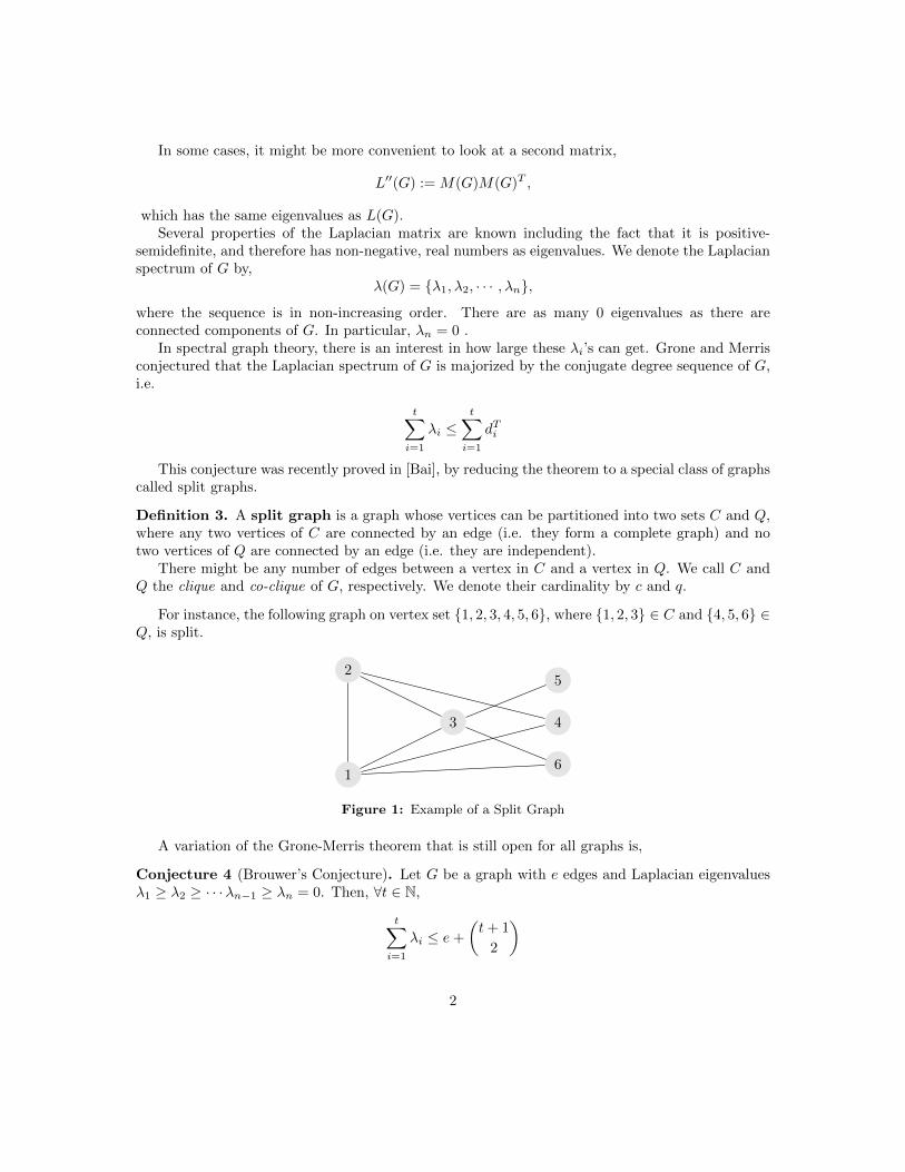
Definition 3. A split graph is a graph whose vertices can be partitioned into two sets C and Q,where any two vertices of C are connected by an edge (i.e. they form a complete graph) and notwo vertices of Q are connected by an edge (i.e. they are independent).

There might be any number of edges between a vertex in C and a vertex in Q. We call C andQ the clique and co-clique of G, respectively. We denote their cardinality by c and q.

For instance, the following graph on vertex set {1, 2, 3, 4, 5, 6}, where {1, 2, 3} ∈ C and {4, 5, 6} ∈Q, is split.

1

2

3 4

5

6

Figure 1: Example of a Split Graph

A variation of the Grone-Merris theorem that is still open for all graphs is,

Conjecture 4 (Brouwer’s Conjecture). Let G be a graph with e edges and Laplacian eigenvaluesλ1 ≥ λ2 ≥ · · ·λn−1 ≥ λn = 0. Then, ∀t ∈ N,

t∑i=1

λi ≤ e+

(t+ 1

2

)

2

It is not hard to see that this conjecture holds for t = 1 and n − 1. It has also been shownfor the second partial sum, and for special classes of graphs including trees, split graphs, regulargraphs, co-graphs, and all graphs with at most 10 vertices.1

Brouwer’s conjecture is intimately connected to the Grone-Merris theorem. Despite the fact thatit uses less information than the Grone-Merris theorem, it is shown in [M] that the t-th inequalityof Brouwer’s conjecture is sharper than that of the Grone-Merris inequality if and only if the graphis non-split.

These conjectures can be generalized to the case of abstract simplicial complexes, which is thetopic of interest for this report.

Definition 5. An (abstract) simplicial complex, S, on a vertex set {1, 2, · · · , n} = [n] is acollection of k-subsets of [n], which are called the faces or simplices, that are closed under inclusion.i.e if F and F ′ are subsets of [n], where F ∈ S and F ′ ⊂ F , then F ′ ∈ S.

Given a face, F , we denote its cardinality by |F |, and its dimension by |F | − 1. The dimensionof a simplicial complex is the maximum dimension of a face in it.

A face F ∈ S is called a facet if dim(F ) = dim(S); and S is called pure if every face in S iscontained in a facet of S. Throughout this report, we assume that all simplicial complexes are pure,undirected, and finite.

Definition 6. The f -vector of S is the sequence

f(S) := (f−1(S), f0(S), f1(S), · · · )

where fi(S) := |Si|.

Given a simplicial complex, S, for all i ∈ N, i ≥ −1, we have chain groups Ci(S) and mapsbetween these chain groups.

0 −→ 0 −→ · · ·C2∂2−→ C1

∂1−→ C0∂0−→ 0

These Ci’s are vector spaces with the basis being the ith dimensional faces of the simplicialcomplex. The ∂’s, which we call the boundary maps, are defined R-linearly by extending thefollowing map on the basis elements.

∂i[v0, · · · , vi] =∑j=0

(−1)j [v0, · · · , v̂j , · · · , vi], (1)

where v0 < v1 < · · · < vi.Here, [v0, · · · , vi] are oriented chains, and so switching any of the vj ’s, where 1 ≤ j ≤ i, switches

the sign. The i − 2-dimensional faces are each multiplied by a sign that depends on the vertex of[v0, · · · , vi] that is removed. In general, for any simplicial complex S and a face {a0, · · · , an} ∈ S(where a0 ≤ a1 ≤ · · · ≤ an), we define the sign of {a0, · · · , an}\{aj} as (−1)j .

We can use (1) to write down these boundary maps matrices. For instance, the boundary map∂2 would have rows indexed by the 2-dimensional faces and the columns by the 1-dimensional faces.

1These proofs can be found in [H] and [M]. We will include the discussion for co-graphs in Section 3.

3

Definition 7. Using the above boundary maps, we can define the following matrices:

L′(S) := ∂k−1∂Tk−1

L′′(S) := ∂Tk−1∂k−1

Note that these definitions agree with those given for graphs. Just as in the graph case, ∂Tk−1∂k−1and ∂k−1∂

Tk−1 have the same non-zero eigenvalues counting multiplicity. Therefore, we may use

either L′(G) or L′′(G) when studying the Laplacian spectrum of simplicial complexes.Before tackling the generalized form of the Grone-Merris theorem and Brouwer’s conjecture, we

note two special classes of simplicial complexes, which the reader might recognize as generalizationsof those given in the graph section.

Definition 8. For a given k, split simplicial complexes are simplicial complexes whose verticescan be divided into a clique and a co-clique.

Just as in the case of graphs, none of the vertices in the co-clique form a k subset of [n] (i.e.they are independent). The clique is a complete simplicial complex. We can have k-dimensionalfaces connecting vertices in the clique to those in the co-clique.2

An example is the simplicial complex S = {123, 124, 134, 234, 235, 237, 246}, for k = 3. Here,{1, 2, 3, 4} ∈ C and {5, 6, 7} ∈ Q.

1 2

345

6

7

Figure 2: Example of a Split Simplicial Complex

Definition 9. A shifted simplicial complex, S, is a simplicial complex in which if F ∈ S, v ⊂ Fand v′ < v, then (F − v) t v′ ∈ S.

We are interested in finding a lower bound for the partial sum of Laplacian eigenvalues ofsimplicial complexes. As such, we will tackle a special case of the generalized Grone-Merris theorem(as conjectured by [DR]).

Conjecture 10. For a simplicial complex, S, with Laplacian spectrum λ(S) = {λ1, λ2, · · · }, thefollowing majorization result holds:

t∑i=1

λi ≤t∑i=1

dTi

This conjecture has been shown for k = 2 (i.e. graphs in [Bai]), shifted simplicial complexes,and for t = 1 (see [DR]).

2We will discuss restrictions on this in Section 2.

4

In Section 2, we present progress made to show the conjecture holds for the second partial sumfor k = 3. Just as in [Bai], we will reduce the conjecture to the case of split simplicial complexes.For a given c and q, we impose a partial ordering on all possible split simplicial complexes, andshow that the conjecture can further be reduced to a subset of these split simplicial complexes.

In Section 3, we present four different possible generalizations of Brouwer’s conjecture, and dis-cuss the progress made to show that these bounds hold for different classes of simplicial complexes.In particular, we will show that one of these is satisfied for all shifted simplicial complexes.

5

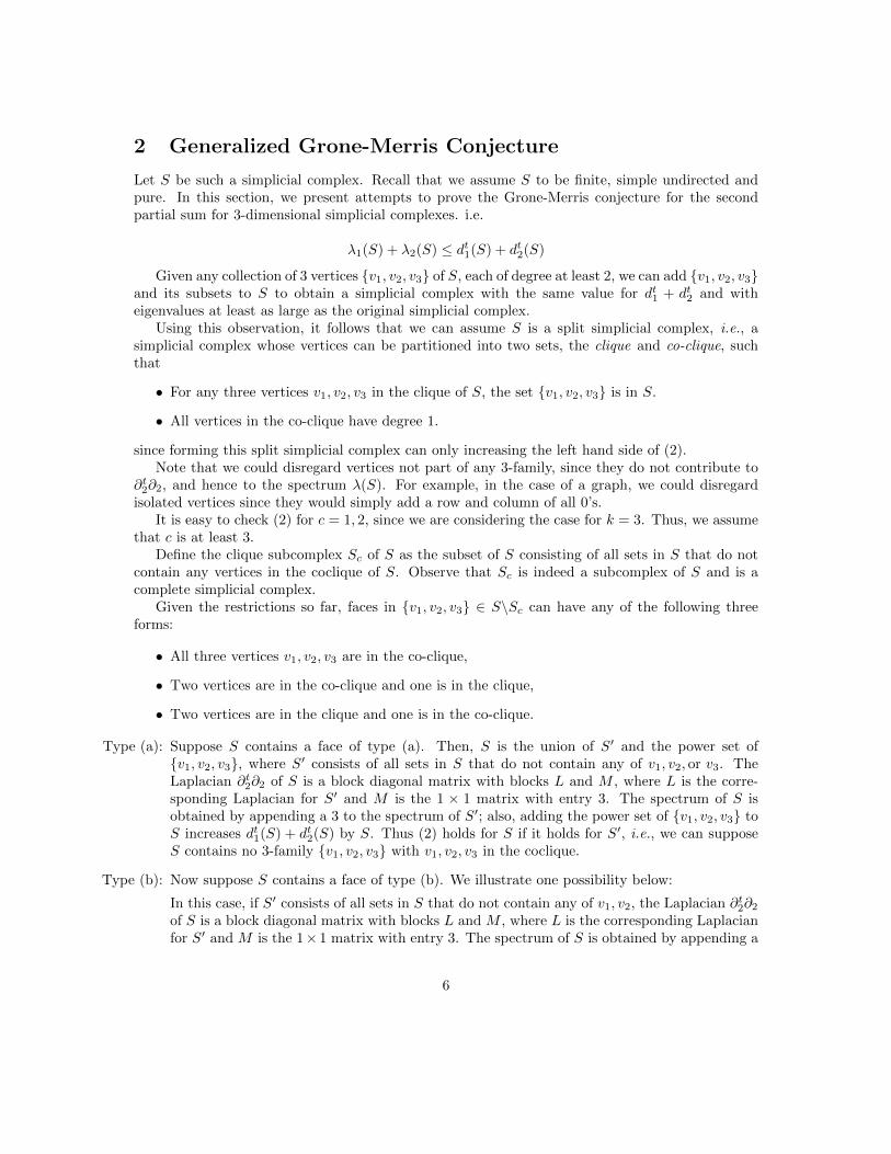
2 Generalized Grone-Merris Conjecture

Let S be such a simplicial complex. Recall that we assume S to be finite, simple undirected andpure. In this section, we present attempts to prove the Grone-Merris conjecture for the secondpartial sum for 3-dimensional simplicial complexes. i.e.

λ1(S) + λ2(S) ≤ dt1(S) + dt2(S)

Given any collection of 3 vertices {v1, v2, v3} of S, each of degree at least 2, we can add {v1, v2, v3}and its subsets to S to obtain a simplicial complex with the same value for dt1 + dt2 and witheigenvalues at least as large as the original simplicial complex.

Using this observation, it follows that we can assume S is a split simplicial complex, i.e., asimplicial complex whose vertices can be partitioned into two sets, the clique and co-clique, suchthat

• For any three vertices v1, v2, v3 in the clique of S, the set {v1, v2, v3} is in S.

• All vertices in the co-clique have degree 1.

since forming this split simplicial complex can only increasing the left hand side of (2).Note that we could disregard vertices not part of any 3-family, since they do not contribute to

∂t2∂2, and hence to the spectrum λ(S). For example, in the case of a graph, we could disregardisolated vertices since they would simply add a row and column of all 0’s.

It is easy to check (2) for c = 1, 2, since we are considering the case for k = 3. Thus, we assumethat c is at least 3.

Define the clique subcomplex Sc of S as the subset of S consisting of all sets in S that do notcontain any vertices in the coclique of S. Observe that Sc is indeed a subcomplex of S and is acomplete simplicial complex.

Given the restrictions so far, faces in {v1, v2, v3} ∈ S\Sc can have any of the following threeforms:

• All three vertices v1, v2, v3 are in the co-clique,

• Two vertices are in the co-clique and one is in the clique,

• Two vertices are in the clique and one is in the co-clique.

Type (a): Suppose S contains a face of type (a). Then, S is the union of S′ and the power set of{v1, v2, v3}, where S′ consists of all sets in S that do not contain any of v1, v2, or v3. TheLaplacian ∂t2∂2 of S is a block diagonal matrix with blocks L and M , where L is the corre-sponding Laplacian for S′ and M is the 1 × 1 matrix with entry 3. The spectrum of S isobtained by appending a 3 to the spectrum of S′; also, adding the power set of {v1, v2, v3} toS increases dt1(S) + dt2(S) by S. Thus (2) holds for S if it holds for S′, i.e., we can supposeS contains no 3-family {v1, v2, v3} with v1, v2, v3 in the coclique.

Type (b): Now suppose S contains a face of type (b). We illustrate one possibility below:

In this case, if S′ consists of all sets in S that do not contain any of v1, v2, the Laplacian ∂t2∂2of S is a block diagonal matrix with blocks L and M , where L is the corresponding Laplacianfor S′ and M is the 1× 1 matrix with entry 3. The spectrum of S is obtained by appending a

6

1 2

345

6

7

5

6

7

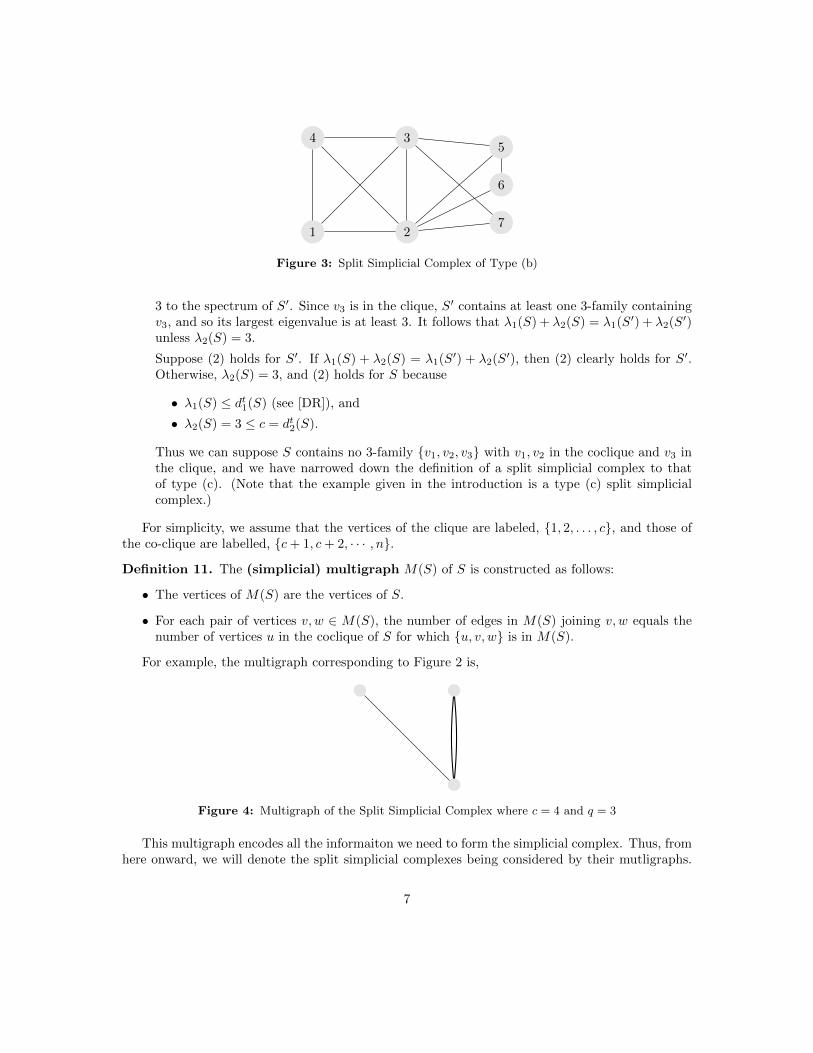
Figure 3: Split Simplicial Complex of Type (b)

3 to the spectrum of S′. Since v3 is in the clique, S′ contains at least one 3-family containingv3, and so its largest eigenvalue is at least 3. It follows that λ1(S) + λ2(S) = λ1(S′) + λ2(S′)unless λ2(S) = 3.

Suppose (2) holds for S′. If λ1(S) + λ2(S) = λ1(S′) + λ2(S′), then (2) clearly holds for S′.Otherwise, λ2(S) = 3, and (2) holds for S because

• λ1(S) ≤ dt1(S) (see [DR]), and

• λ2(S) = 3 ≤ c = dt2(S).

Thus we can suppose S contains no 3-family {v1, v2, v3} with v1, v2 in the coclique and v3 inthe clique, and we have narrowed down the definition of a split simplicial complex to thatof type (c). (Note that the example given in the introduction is a type (c) split simplicialcomplex.)

For simplicity, we assume that the vertices of the clique are labeled, {1, 2, . . . , c}, and those ofthe co-clique are labelled, {c+ 1, c+ 2, · · · , n}.

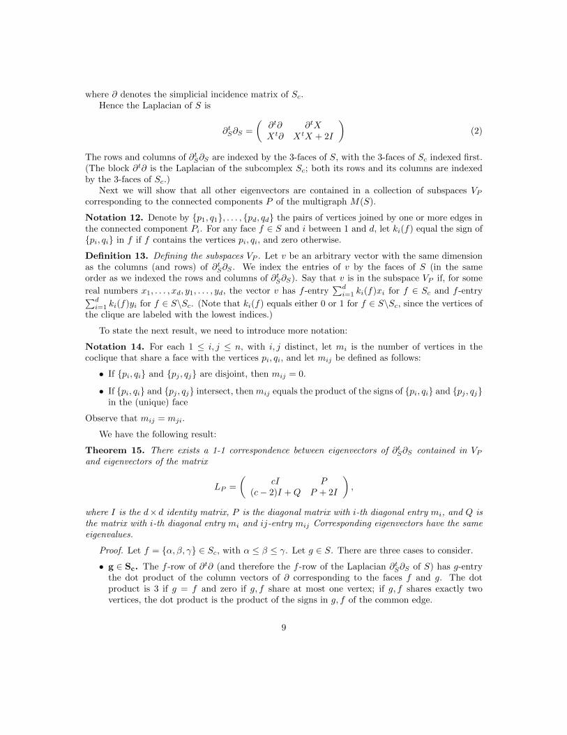
Definition 11. The (simplicial) multigraph M(S) of S is constructed as follows:

• The vertices of M(S) are the vertices of S.

• For each pair of vertices v, w ∈ M(S), the number of edges in M(S) joining v, w equals thenumber of vertices u in the coclique of S for which {u, v, w} is in M(S).

For example, the multigraph corresponding to Figure 2 is,

Figure 4: Multigraph of the Split Simplicial Complex where c = 4 and q = 3

This multigraph encodes all the informaiton we need to form the simplicial complex. Thus, fromhere onward, we will denote the split simplicial complexes being considered by their mutligraphs.

7

After fixing the clique and co-clique size, we can put a partial ordering of all the possible simplicialeigenvalues using the first and second partial sum of their Laplacian eigenvalues, which we canshow using these multigraphs.3 For example, if we fix c = 4 and q = 4, we get nine different splitsimplicial complexes ordered as,

(8, 4)

(6.449, 5.414) (7, 5)

(7.057, 4.827) (6, 6)

(6.164, 5.303)

(6.112, 5.212)

(5.562, 5.303)

(5.562, 5)

Figure 5: Poset of Split Simplicial Complexes for c = 4 and q = 4

The simplicial incidence matrix ∂S of S has the form ∂ X0 I0 −I

3See Appendix A for more examples.

8

where ∂ denotes the simplicial incidence matrix of Sc.Hence the Laplacian of S is

∂tS∂S =

(∂t∂ ∂tXXt∂ XtX + 2I

)(2)

The rows and columns of ∂tS∂S are indexed by the 3-faces of S, with the 3-faces of Sc indexed first.(The block ∂t∂ is the Laplacian of the subcomplex Sc; both its rows and its columns are indexedby the 3-faces of Sc.)

Next we will show that all other eigenvectors are contained in a collection of subspaces VPcorresponding to the connected components P of the multigraph M(S).

Notation 12. Denote by {p1, q1}, . . . , {pd, qd} the pairs of vertices joined by one or more edges inthe connected component Pi. For any face f ∈ S and i between 1 and d, let ki(f) equal the sign of{pi, qi} in f if f contains the vertices pi, qi, and zero otherwise.

Definition 13. Defining the subspaces VP . Let v be an arbitrary vector with the same dimensionas the columns (and rows) of ∂tS∂S . We index the entries of v by the faces of S (in the sameorder as we indexed the rows and columns of ∂tS∂S). Say that v is in the subspace VP if, for some

real numbers x1, . . . , xd, y1, . . . , yd, the vector v has f -entry∑di=1 ki(f)xi for f ∈ Sc and f -entry∑d

i=1 ki(f)yi for f ∈ S\Sc. (Note that ki(f) equals either 0 or 1 for f ∈ S\Sc, since the vertices ofthe clique are labeled with the lowest indices.)

To state the next result, we need to introduce more notation:

Notation 14. For each 1 ≤ i, j ≤ n, with i, j distinct, let mi is the number of vertices in thecoclique that share a face with the vertices pi, qi, and let mij be defined as follows:

• If {pi, qi} and {pj , qj} are disjoint, then mij = 0.

• If {pi, qi} and {pj , qj} intersect, then mij equals the product of the signs of {pi, qi} and {pj , qj}in the (unique) face

Observe that mij = mji.

We have the following result:

Theorem 15. There exists a 1-1 correspondence between eigenvectors of ∂tS∂S contained in VPand eigenvectors of the matrix

LP =

(cI P

(c− 2)I +Q P + 2I

),

where I is the d× d identity matrix, P is the diagonal matrix with i-th diagonal entry mi, and Q isthe matrix with i-th diagonal entry mi and ij-entry mij Corresponding eigenvectors have the sameeigenvalues.

Proof. Let f = {α, β, γ} ∈ Sc, with α ≤ β ≤ γ. Let g ∈ S. There are three cases to consider.

• g ∈ Sc. The f -row of ∂t∂ (and therefore the f -row of the Laplacian ∂tS∂S of S) has g-entrythe dot product of the column vectors of ∂ corresponding to the faces f and g. The dotproduct is 3 if g = f and zero if g, f share at most one vertex; if g, f shares exactly twovertices, the dot product is the product of the signs in g, f of the common edge.

9

• g = {pi,qi, c} ∈ S\Sc for some 1 ≤ i ≤ d. The g-column of ∂tX is just the row of ∂ corre-sponding to {pi, qi}; hence the f -row of the Laplacian ∂tS∂S has g-entry ki(f).

• g ∈ S\Sc but does not contain the pair {pi,qi} for any i. The f -row g-column entry ofthe Laplacian ∂tS∂S will not affect future calculations, since vectors in VP have g-entry zero.

Thus, for a vector v ∈ VP , its image ∂S∂tSv under the Laplacian map has f -entry

3∑i

ci(f)xi +∑

g={α,β,δ},δ 6=γ∈Sc

(sign of {α, β} in g)∑i

ki(g)xi

−∑

g={α,γ,δ},δ 6=β∈Sc

(sign of {α, γ} in g)∑i

ki(g)xi

+∑

g={β,γ,δ},δ 6=α∈Sc

(sign of {β, γ} in g)∑i

ki(g)xi

+

d∑i=1

miki(f)yi,

where mi is the number of vertices in the coclique that share a face with the vertices pi, qi. Let1 ≤ i ≤ d be arbitrary.

• If f contains neither pi nor qi, then ki(g) = 0 for all faces g sharing at least two vertices withf ; so xi must have coefficient zero.

• Suppose that f contains pi but not qi. If pi = β, then xi has coefficient

(sign of {α, β} in {α, β, qi})ki ({α, β, qi}) + (sign of {β, γ} in {β, γ, qi})ki ({β, γ, qi})= (sign of {α, β} in {α, β, qi}) · (sign of {β, qi} in {α, β, qi})

+ (sign of {β, γ} in {β, γ, qi}) · (sign of {β, qi} in {β, γ, qi})= −(sign of {α, qi} in {α, β, qi})− (sign of {γ, qi} in {β, γ, qi})

If β < qi then {α, qi} has sign −1 in {α, β, qi} and {γ, qi} has sign 1 in {β, γ, qi}; if β > qi then{α, qi} has sign 1 in {α, β, qi} and {γ, qi} has sign −1 in {β, γ, qi}. Hence xi has coefficientzero. Similar reasoning shows xi has coefficient zero when pi equals either α or γ.

• Finally, suppose that f contains both pi and qi. Then xi has coefficient

3ki(f) +∑

g={pi,qi,δ},δ∈Sc\f

(sign of {pi, qi} in f)(sign of {pi, qi} in g)ki(g)xi

or cki(f).

We deduce that ∂S∂tSv has f -entry

d∑i=1

cki(f)xi +

d∑i=1

miki(f)yi (3)

10

Now suppose f = {α, β, γ} with γ in the coclique. Then, for g ∈ Sc, the g-entry of the f -rowof ∂S∂

tS is the sign of {α, β} in g. For g ∈ S\Sc, the g-entry of the f -row of ∂S∂

tS is 3 if g = f , 1

if g 6= f but {α, β} ∈ g, and 0 otherwise. Thus, for a vector v ∈ VP , its image ∂S∂tSv under the

Laplacian map has f -entry

∑g∈Sc

(sign of {α, β} in g)

(∑i

ki(g)xi

)+ (mi + 2)yi (4)

If {α, β} is not in P , but in a different component of the multigraph M(S), then ki(g) and thesign of {α, β} in g cannot both be nonzero. If {α, β} is in P , then the sign of {α, β} in g is just∑j kj(f)kj(g). Therefore (4) reduces to

∑g∈Sc

∑j

kj(f)kj(g)

(∑i

ki(g)xi

)+ (mi + 2)yi (5)

Fix 1 ≤ j ≤ d. Let gi be the element of Sc containing both {pi, qi} and {pj , qj} for each 1 ≤ i ≤ dfor which such a gi exists. (If no such gi exists for some i, let gi be an arbitrary face; it does notmatter.) Observe that the gi are not necessarily pairwise distinct. The expression (5) is just∑

j

(c− 2)kj(f)xj +∑i6=j

∑j

kj(f)kj(gi)ki(gi)xi + (mi + 2)yi

or ∑i

∑j

kj(f)mijxi + (mi + 2)yi, (6)

where mij is defined as follows:

• If {pi, qi} and {pj , qj} are disjoint, then mij = 0.

• If {pi, qi} and {pj , qj} intersect, then mij equals the product of the signs of {pi, qi} and {pj , qj}in the (unique) face

Suppose that the vector v′ = (x1 x2 · · · xd y1 y2 · · · yd) is an eigenvector of the matrix ... witheigenvalue λ. Then

λxi = cxi +miyi

andλyi = (c− 2)xi +

∑j 6=i

mijxj + (mi + 2)yi,

and the expressions (3) and (6) become∑i λki(f)xi and

∑i λki(f)yi, respectively. We conclude

that, if v′ is an eigenvector of the matrix LP , then v is an eigenvector of the matrix LP . Since thematrix LP is just the restriction of the Laplacian ∂S∂

tS to the subspace VP the matrix LP has a

basis of eigevectors. These eigenvectors correspond to 2d eigenvectors of ∂S∂tS in VP . Since VP has

dimension 2d, we see that every eigenvector of ∂S∂tS in VP corresponds to an eigenvector of the

matrix LP with the same eigenvalue. �

11

3 Generalized Brouwer’s Conjecture

First, we discuss the proofs of Brouwer’s conjecture for some special classes of graphs, which willcome in handy in the following sub-sections. We will then detail different possible generalizationsof Brouwer’s conjecture to the case of simplical complexes.

3.1 Brouwer’s Conjecture for Graphs

First, we note two ways to obtain new graphs from old ones in such a way that the Laplacianeigenvalues of the new graph can be easily extracted from the old ones.

Given two graphs, G1 and G2, we can obtain their disjoint union, G1 tG2, by simply takingthe union of their vertices and edges. The Laplacian spectrum of this new graph is simply the directsum of the Laplacian spectra of G1 and G2.

The complement of G, Gc, is the graph that has two vertices being adjacent if and only ifthey were not adjacent in G. If the Laplacian spectrum of G in non-increasing order is, λ1 ≥ λ2 ≥· · · ≥ λn, then that of Gc is 0 ≤ n− λn−1 ≤ · · · ≤ n− λ1 in non-decreasing order, which we relabelas λc1 ≤ · · · ≤ λcn−1 ≤ λcn = 0.

3.1.1 Co-graphs

Definition 16. A cograph is a graph that does not contain P4, the path graph on four vertices,as a subgraph.

There is an inductive way of defining co-graphs, using the following rules.

• a single vertex is a cograph

• if G is a cograph, then so is Gc

• if G1 and G2 are cographs, then so is G1 tG2

We note the following lemmata, whose proofs can be found in [M], or can easily be reproducedby noting how the Laplacian spectrum changes when considering the complement graph and thedisjoint union of two graphs.

Lemma 17. A graph G satisfies Brouwer’s conjecture if and only if Gc also satisfies Brouwer’sconjecture.

Lemma 18. If two graphs, G1 and G2 satisfy Brouwer’s conjecture, so does G1 tG2.

Lemma 19. Cographs satisfy Brouwer’s conjecture.

Proof. This easily follows from the fact that the single vertex satisfies Brouwer’s conjecture, Lemma17 and Lemma 18.

Definition 20. A threshold graph is a special type of co-graph that can be defined inductivelyas follows.

• Isolated points are threshold graphs.

12

• A graph on n vertices is threshold if some subgraph of n−1 vertices is threshold and the n-thremaining vertex is either an isolated vertex or a cone vertex (i.e., a vertex connected to allother vertices by an edge).

Threshold graphs are a special type of co-graphs. Two special cases of threshold graphs are thecomplete graph and the star graph. The former is obtained by adding a cone vertex at each stageand the latter by adding n − 1 empty vertices and a final cone vertex. Threshold graphs clearlysatisfy Brouwer’s conjecture as they are co-graphs. We can, in fact, deduce a stronger result forthreshold graphs.

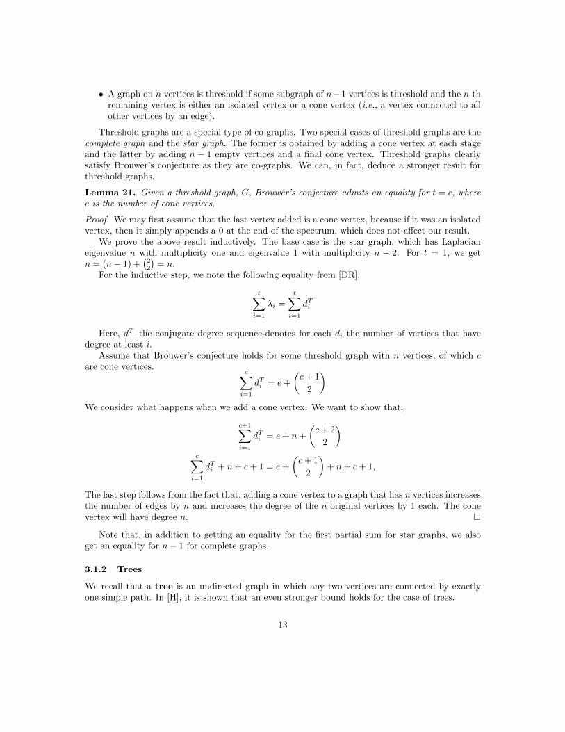
Lemma 21. Given a threshold graph, G, Brouwer’s conjecture admits an equality for t = c, wherec is the number of cone vertices.

Proof. We may first assume that the last vertex added is a cone vertex, because if it was an isolatedvertex, then it simply appends a 0 at the end of the spectrum, which does not affect our result.

We prove the above result inductively. The base case is the star graph, which has Laplacianeigenvalue n with multiplicity one and eigenvalue 1 with multiplicity n − 2. For t = 1, we getn = (n− 1) +

(22

)= n.

For the inductive step, we note the following equality from [DR].

t∑i=1

λi =

t∑i=1

dTi

Here, dT –the conjugate degree sequence-denotes for each di the number of vertices that havedegree at least i.

Assume that Brouwer’s conjecture holds for some threshold graph with n vertices, of which care cone vertices.

c∑i=1

dTi = e+

(c+ 1

2

)We consider what happens when we add a cone vertex. We want to show that,

c+1∑i=1

dTi = e+ n+

(c+ 2

2

)c∑i=1

dTi + n+ c+ 1 = e+

(c+ 1

2

)+ n+ c+ 1,

The last step follows from the fact that, adding a cone vertex to a graph that has n vertices increasesthe number of edges by n and increases the degree of the n original vertices by 1 each. The conevertex will have degree n.

Note that, in addition to getting an equality for the first partial sum for star graphs, we alsoget an equality for n− 1 for complete graphs.

3.1.2 Trees

We recall that a tree is an undirected graph in which any two vertices are connected by exactlyone simple path. In [H], it is shown that an even stronger bound holds for the case of trees.

13

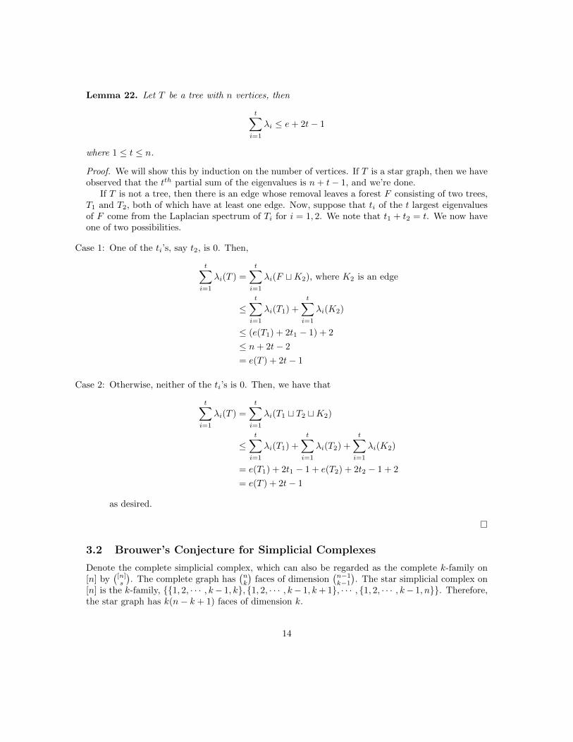
Lemma 22. Let T be a tree with n vertices, then

t∑i=1

λi ≤ e+ 2t− 1

where 1 ≤ t ≤ n.

Proof. We will show this by induction on the number of vertices. If T is a star graph, then we haveobserved that the tth partial sum of the eigenvalues is n+ t− 1, and we’re done.

If T is not a tree, then there is an edge whose removal leaves a forest F consisting of two trees,T1 and T2, both of which have at least one edge. Now, suppose that ti of the t largest eigenvaluesof F come from the Laplacian spectrum of Ti for i = 1, 2. We note that t1 + t2 = t. We now haveone of two possibilities.

Case 1: One of the ti’s, say t2, is 0. Then,

t∑i=1

λi(T ) =

t∑i=1

λi(F tK2), where K2 is an edge

≤t∑i=1

λi(T1) +

t∑i=1

λi(K2)

≤ (e(T1) + 2t1 − 1) + 2

≤ n+ 2t− 2

= e(T ) + 2t− 1

Case 2: Otherwise, neither of the ti’s is 0. Then, we have that

t∑i=1

λi(T ) =

t∑i=1

λi(T1 t T2 tK2)

≤t∑i=1

λi(T1) +

t∑i=1

λi(T2) +

t∑i=1

λi(K2)

= e(T1) + 2t1 − 1 + e(T2) + 2t2 − 1 + 2

= e(T ) + 2t− 1

as desired.

3.2 Brouwer’s Conjecture for Simplicial Complexes

Denote the complete simplicial complex, which can also be regarded as the complete k-family on[n] by

([n]s

). The complete graph has

(nk

)faces of dimension

(n−1k−1). The star simplicial complex on

[n] is the k-family, {{1, 2, · · · , k− 1, k}, {1, 2, · · · , k− 1, k+ 1}, · · · , {1, 2, · · · , k− 1, n}}. Therefore,the star graph has k(n− k + 1) faces of dimension k.

14

The lexicographic ordering of the faces in simplicial complexes allows us to see a special propertyof shifted simplicial complexes called shelling.

Definition 23. Shelling is a way to build a simplicial complex one facet at a time, so that eachfacet added includes a new minimal face to the simplicial complex. The lexicographic order of thefaces induces a canonical shelling order.

One can check for shiftedness of a simplicial complex, S, by taking the complete simplicialcomplex on the same vertices and looking at the partially ordered set of its faces in lexicographicorder, P . Take the sub-poset induced by S, PS , and look at its maximal elements, mi. If ∀pi ∈P, pi ≤ mi, we have that pi ∈ PS , then S is shifted.

Just as in the case of graphs, there are operations that allow us to construct new simplicialcomplexes from old ones such that the Laplacian eigenvalues change in a predictable manner. Wenote the following equalities from [DR]:

Given two simplicial complexes, S1 and S2, the Laplacian spectra of S1tS2 is simply the directsum of the Laplacian spectra of S1 and S2.

The complement of S, which we will denote by Sc, is

Sc :=

([n]

k

)\S = {F ⊆ [n] : |F | = k, F /∈ S}

and the star of S, which we will denote by S∗, is

S∗ := {[n]\S : F ∈ S}

The complement of S is a k-family while S∗ is an (n− k)-family. Moreover, both the star andthe complementation operation are involutive ((Sc)c = (S∗)∗ = S) and they also commute withone another (Sc∗ = S∗c).

These final two operations affect the Laplacian spectra in the following way. If S has Laplacianspectrum,

λ = (λ1, λ2, · · · )

then the Laplacian spectrum of S∗ is

λ∗i = n− λ|S|+1−i

and the Laplacian spectrum of Sc is

λci = n− λ(n−1k−1)+1−i

We can finally present the different possible generalizations of Brouwer’s conjecture. For eachof the possible forms, we note the progress that has been made to show that the bounds holdsfor special classes of simplicial complexes, and also under the different operations on simplicialcomplexes. No counter examples have been found from the SAGE computations for any of thesebounds.

15

3.2.1 Possible Generalization I

(t+k−2k−1 )∑i=1

λi ≤ fk−1 + (k − 1)

(t+ k − 1

k

)When considering the graph case, we let k = 2, and the generalized form reduces to Brouwer’s

conjecture that we saw earlier in this report. This generalized bound preserves some of the propertiesthat we’ve already seen.

Lemma 24. The star simplicial complex on [n] for all k ≥ 2 satisfies generalized Brouwer’s con-jecture I, and with equality for t = 1.

Proof. The star simplicial complex, S, has Laplacian spectra of the following form:

λ(S) = {n}1, {k}n−k

We prove the statement inductively. The base case clearly gives an equality. Now, assume thegeneralized bound holds for some partial sum s ≥ 1. i.e

n+ sk = (n− k + 1) + (k − 1)

(s+ k − 1

k

)We want to show that

n+ (s+ 1)k ≤ (n− k + 1) + (k − 1)

(s+ k

k

)n+ sk + k ≤ (n− k + 1) + (k − 1)

(s+ k − 1

k − 1

)+ (k − 1)

(s+ k − 1

k

)k ≤ (k − 1)

(s+ k − 1

k − 1

)which is clearly true.

Lemma 25. The complete simplicial complex satisfies generalized Brouwer’s conjecture I, and withequality for t = n− k + 1

Proof. Note that the complete simplicial complex, S, has Laplacian spectra of the form

λ(S) = n(n−1k−1)

For t = n− k + 1, generalized Brouwer’s conjecture states that

n

(n− 1

k − 1

)=

(n

k

)+ (k − 1)

(n

k

)=

(n

k

)+ (k)

(n

k

)−(n

k

)= n

(n− 1

k − 1

)

16

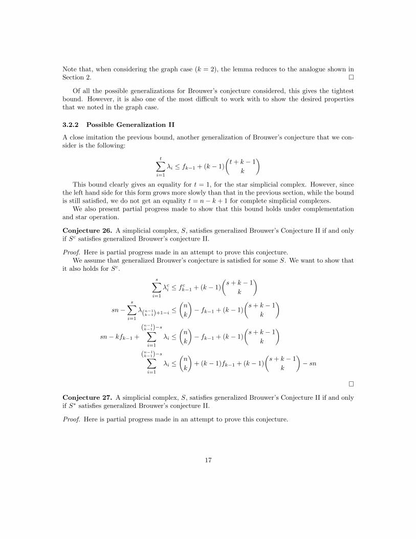
Note that, when considering the graph case (k = 2), the lemma reduces to the analogue shown inSection 2.

Of all the possible generalizations for Brouwer’s conjecture considered, this gives the tightestbound. However, it is also one of the most difficult to work with to show the desired propertiesthat we noted in the graph case.

3.2.2 Possible Generalization II

A close imitation the previous bound, another generalization of Brouwer’s conjecture that we con-sider is the following:

t∑i=1

λi ≤ fk−1 + (k − 1)

(t+ k − 1

k

)This bound clearly gives an equality for t = 1, for the star simplicial complex. However, since

the left hand side for this form grows more slowly than that in the previous section, while the boundis still satisfied, we do not get an equality t = n− k + 1 for complete simplicial complexes.

We also present partial progress made to show that this bound holds under complementationand star operation.

Conjecture 26. A simplicial complex, S, satisfies generalized Brouwer’s Conjecture II if and onlyif Sc satisfies generalized Brouwer’s conjecture II.

Proof. Here is partial progress made in an attempt to prove this conjecture.We assume that generalized Brouwer’s conjecture is satisfied for some S. We want to show that

it also holds for Sc.

s∑i=1

λci ≤ f ck−1 + (k − 1)

(s+ k − 1

k

)

sn−s∑i=1

λ(n−1k−1)+1−i ≤

(n

k

)− fk−1 + (k − 1)

(s+ k − 1

k

)

sn− kfk−1 +

(n−1k−1)−s∑i=1

λi ≤(n

k

)− fk−1 + (k − 1)

(s+ k − 1

k

)(n−1k−1)−s∑i=1

λi ≤(n

k

)+ (k − 1)fk−1 + (k − 1)

(s+ k − 1

k

)− sn

Conjecture 27. A simplicial complex, S, satisfies generalized Brouwer’s Conjecture II if and onlyif S∗ satisfies generalized Brouwer’s conjecture II.

Proof. Here is partial progress made in an attempt to prove this conjecture.

17

We assume that generalized Brouwer’s conjecture is satisfied for some S, and we want to showthat it holds for S∗.

s∑i=1

λ∗i ≤ f∗k−1 + (n− k − 1)

(s+ n− k − 1

n− k

)

sn−s∑i=1

λ|k|+1−i ≤ fk−1 + (n− k − 1)

(s+ n− k − 1

n− k

)

sn− kfk−1 +

|k|−s∑i=1

λi ≤ fk−1 + (n− k − 1)

(s+ n− k − 1

n− k

)|k|−s∑i=1

λi ≤ (k + 1)fk−1 + (n− k − 1)

(s+ n− k − 1

n− k

)

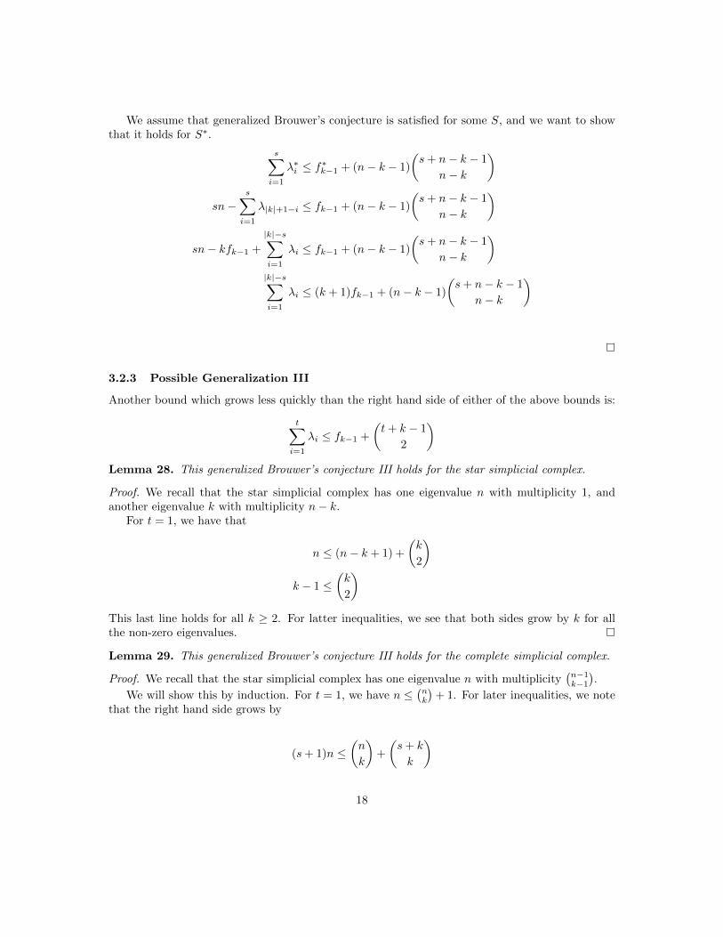
3.2.3 Possible Generalization III

Another bound which grows less quickly than the right hand side of either of the above bounds is:

t∑i=1

λi ≤ fk−1 +

(t+ k − 1

2

)Lemma 28. This generalized Brouwer’s conjecture III holds for the star simplicial complex.

Proof. We recall that the star simplicial complex has one eigenvalue n with multiplicity 1, andanother eigenvalue k with multiplicity n− k.

For t = 1, we have that

n ≤ (n− k + 1) +

(k

2

)k − 1 ≤

(k

2

)This last line holds for all k ≥ 2. For latter inequalities, we see that both sides grow by k for allthe non-zero eigenvalues.

Lemma 29. This generalized Brouwer’s conjecture III holds for the complete simplicial complex.

Proof. We recall that the star simplicial complex has one eigenvalue n with multiplicity(n−1k−1).

We will show this by induction. For t = 1, we have n ≤(nk

)+ 1. For later inequalities, we note

that the right hand side grows by

(s+ 1)n ≤(n

k

)+

(s+ k

k

)

18

For t =(n−1k−1), we have that

n

(n− 1

k − 1

)≤(n

k

)+

(k

2

)k − 1 ≤

(k

2

)This last line holds for all k ≥ 2. For latter inequalities, we see that both sides grow by k for allthe non-zero eigenvalues.

While a simpler form than the previous generalized bounds, this bound is not any easier to workwith when trying to show that it holds under complementation and star operation.

3.2.4 Possible Generalization IV

t∑i=1

λi ≤ (k − 1)fk−1 +

(t+ k − 1

k

)For this bound does not given an equality for the complete simplicial complex for t =

(n−1k−1)

(take the the complete simplicial complex on 4 vertices for k=3, for example) or the star simplicialcomplex for t = 1 (the star simplicial complex on 4 vertices for k=3 is a counter example). However,the bound holds for all shifted simplicial complexes.

Theorem 30. Shifted simplicial complexes satisfy Brouwer’s conjecture for simplicial complexes.

Proof. First, recall that shifted simplicial complexes are shellable. The lexicographic order on thefaces gives us a canonical shelling. Moreover, for shifted simplicial complexes, we have that,

t∑i=1

λi =

t∑i=1

dTi

where dTi is the conjugate degree transpose.Now, assume that Brouwer’s conjecture for simplicial complexes is not satisfied for some t and

k. We choose a minimal counterexample, S, for which this bound is not satisfied. That is, whileS does not satisfy Brouwer’s conjecture, if you remove any of its maximal faces, F , then the newsimplicial complex, S\F does. (Note that F must be maximal, because if it was not, then our newsimplicial complex would no longer be shifted.) We have two cases:

Case 1: S has ≥ t+ k verticesThere exists a maximal face F = {v1, v2, · · · , vk} where v1 ≥ v2 ≥ · · · ≥ vk, such that vk isat least t + k. To see this, choose any face such that vk ≥ t + k. If it is maximal, then weare done. If it is not, then we can increase the indices by going up the partially ordered setuntil we reach a maximal element. Relabel this face F = {v1, v2, · · · , vk}. We will still havethat vk ≥ t + k since going up the partially ordered set can only increase the indices of thevertices.

Since S is shifted, it follows that it contains F ′ = {v1, v2, · · · , vk−1, vk′} for all v′k < vk, suchthat the cardinality of F ′ is still k. Thus, each of {v1, v2, · · · , vk−1} has degree at least t+ 1.

19

We delete F from our simplicial complex, to get S\F . This reduces the degrees of {v1, v2, · · · , vk−1}by one each. Thus, when we delete F the left hand side of the bound goes down by less thank < 1, while the right hand side goes down by exactly k − 1. Thus, if S\F had satisfied thebound, then S should as well, and we reach a contradiction.

Case 2: S has < t+ k vertices

fk−1 ≤(t+ k − 1

k

)(k − 1)fk−1 + fk−1 ≤

(t+ k − 1

k

)+ (k − 1)fk−1

kfk−1 ≤(t+ k − 1

k

)+ (k − 1)fk−1∑

λ ≤(t+ k − 1

k

)+ (k − 1)fk−1

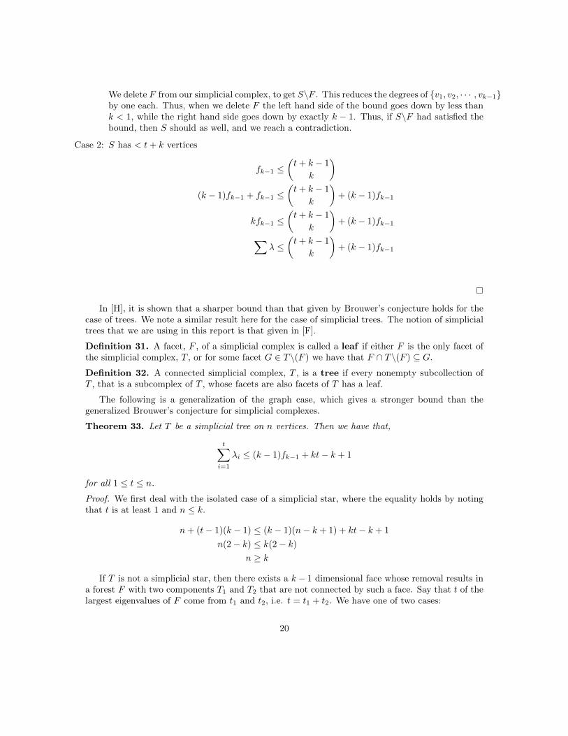
In [H], it is shown that a sharper bound than that given by Brouwer’s conjecture holds for thecase of trees. We note a similar result here for the case of simplicial trees. The notion of simplicialtrees that we are using in this report is that given in [F].

Definition 31. A facet, F , of a simplicial complex is called a leaf if either F is the only facet ofthe simplicial complex, T , or for some facet G ∈ T\(F ) we have that F ∩ T\(F ) ⊆ G.

Definition 32. A connected simplicial complex, T , is a tree if every nonempty subcollection ofT , that is a subcomplex of T , whose facets are also facets of T has a leaf.

The following is a generalization of the graph case, which gives a stronger bound than thegeneralized Brouwer’s conjecture for simplicial complexes.

Theorem 33. Let T be a simplicial tree on n vertices. Then we have that,

t∑i=1

λi ≤ (k − 1)fk−1 + kt− k + 1

for all 1 ≤ t ≤ n.

Proof. We first deal with the isolated case of a simplicial star, where the equality holds by notingthat t is at least 1 and n ≤ k.

n+ (t− 1)(k − 1) ≤ (k − 1)(n− k + 1) + kt− k + 1

n(2− k) ≤ k(2− k)

n ≥ k

If T is not a simplicial star, then there exists a k − 1 dimensional face whose removal results ina forest F with two components T1 and T2 that are not connected by such a face. Say that t of thelargest eigenvalues of F come from t1 and t2, i.e. t = t1 + t2. We have one of two cases:

20

Case 1: One of the ti’s, say t2, is 0, i.e t1 = t.

t∑i=1

λi(T ) =

t∑i=1

λi(F tKk), where Kk is one k face

≤t∑i=1

λi(T1) +

t∑i=1

λi(Kk)

≤ (k − 1)fk−1(T1) + kt1 − k + 1 + k

≤ (k − 1)fk−1(T ) + kt− 1

as desired.

Case 2: Otherwise, neither of the ti’s is 0. Then, we have that

t∑i=1

λi(T ) =

t∑i=1

λi(T1 t T2 tKk)

≤t∑i=1

λi(T1) +

t∑i=1

λi(T2) +

t∑i=1

λi(Kk)

≤ (k − 1)fk−1(T1) + (k − 1)fk−1(T2) + kt1 + kt2 − k + 2

≤ (k − 1)fk−1(T ) + kt− k + 2

which also holds.

21

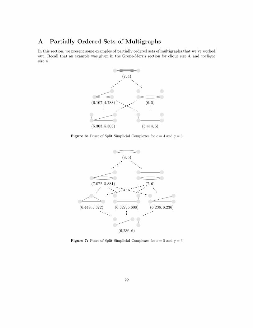
A Partially Ordered Sets of Multigraphs

In this section, we present some examples of partially ordered sets of multigraphs that we’ve workedout. Recall that an example was given in the Grone-Merris section for clique size 4, and cocliquesize 4.

(7, 4)

(6.107, 4.788) (6, 5)

(5.414, 5)(5.303, 5.303)

Figure 6: Poset of Split Simplicial Complexes for c = 4 and q = 3

(8, 5)

(7.072, 5.881) (7, 6)

(6.327, 5.608) (6.236, 6.236)(6.449, 5.372)

(6.236, 6)

Figure 7: Poset of Split Simplicial Complexes for c = 5 and q = 3

22

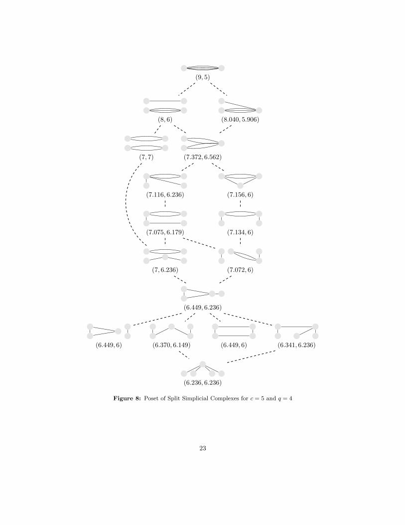
(9, 5)

(8, 6) (8.040, 5.906)

(7.372, 6.562)(7, 7)

(7.156, 6)(7.116, 6.236)

(7.134, 6)(7.075, 6.179)

(7.072, 6)(7, 6.236)

(6.449, 6.236)

(6.449, 6) (6.370, 6.149) (6.449, 6) (6.341, 6.236)

(6.236, 6.236)

Figure 8: Poset of Split Simplicial Complexes for c = 5 and q = 4

23

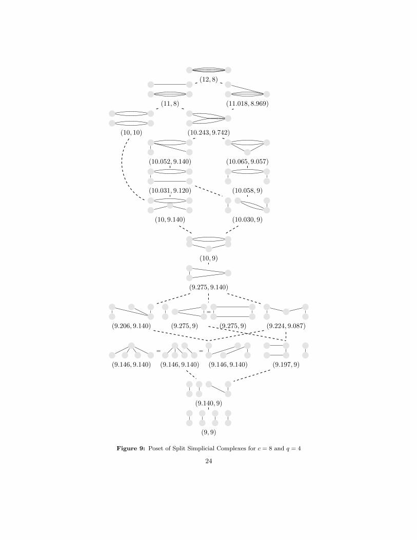
(12, 8)

(11, 8) (11.018, 8.969)

(10.243, 9.742)(10, 10)

(10.065, 9.057)(10.052, 9.140)

(10.058, 9)(10.031, 9.120)

(10, 9.140) (10.030, 9)

(10, 9)

(9.275, 9.140)

(9.206, 9.140) (9.275, 9) (9.275, 9) (9.224, 9.087)

(9.146, 9.140) (9.146, 9.140)(9.146, 9.140) (9.197, 9)

(9.140, 9)

(9, 9)

Figure 9: Poset of Split Simplicial Complexes for c = 8 and q = 4

24

References

[Bai] H. Bai: The Grone-Merris Conjecture. Transactions of the American Mathematical Society.363, 2011.

[BH] A.E. Brouwer and W.E. Haemers: Spectra of Graphs. Springer UTM, Springer, 2012.

[DR] A. Duval and V. Reiner: Shifted Simplicial Complexes are Laplacian Integral. Transactions ofthe American Mathematicial Society, 2002.

[F] S. Faridi: Simplicial Trees: Properties and Applications.

[H] W.H. Haemers, A. Mohammadian, and B. Tayfeh-Rezaie: On the Sum of Laplacian Eigenval-ues of Graphs. Discussion Paper 2008-98, Tilburg University, Center for Economic Research.

[M] Mayank: On Variants of the Grone-Merris Conjecture. Master’s Thesis, Eindhoven Universityof Technology, November 2010.

25