on the resilience of biometric authentication systems
TRANSCRIPT

On the Resilience of Biometric AuthenticationSystems against Random Inputs
Benjamin Zi Hao ZhaoUniversity of New South Wales
and Data61 [email protected]
Hassan Jameel AsgharMacquarie Universityand Data61 CSIRO
Mohamed Ali KaafarMacquarie Universityand Data61 CSIRO
Abstract—We assess the security of machine learning basedbiometric authentication systems against an attacker who submitsuniform random inputs, either as feature vectors or raw inputs,in order to find an accepting sample of a target user. The averagefalse positive rate (FPR) of the system, i.e., the rate at which animpostor is incorrectly accepted as the legitimate user, may beinterpreted as a measure of the success probability of such anattack. However, we show that the success rate is often higher thanthe FPR. In particular, for one reconstructed biometric systemwith an average FPR of 0.03, the success rate was as high as0.78. This has implications for the security of the system, as anattacker with only the knowledge of the length of the feature spacecan impersonate the user with less than 2 attempts on average.We provide detailed analysis of why the attack is successful, andvalidate our results using four different biometric modalities andfour different machine learning classifiers. Finally, we proposemitigation techniques that render such attacks ineffective, withlittle to no effect on the accuracy of the system.
I. INTRODUCTION
Consider a machine learning model trained on some user’sdata accessible as a black-box API for biometric authentica-tion. Given an input (a biometric sample), the model outputsa binary decision, i.e., accept or reject, as its prediction forwhether the input belongs to the target user or not. Nowimagine an attacker with access to the same API who has neverobserved the target user’s inputs. The goal of the attacker is toimpersonate the user by finding an accepting sample (input).What is the success probability of such an attacker?
Biometric authentication systems are generally based on ei-ther physiological biometrics such as fingerprints [1], face [2],[3], and voice [4], [5]), or behavioral biometrics such astouch [6] and gait [7], the latter category generally used forcontinuous and implicit authentication of users. These systemsare mostly based on machine learning: a binary classifier istrained on the target user’s data (positive class) and a subsetof data from other users (negative class). This process is usedto validate the performance of the machine learning classifierand hence the biometric system [8], [7], [9], [10], [11], [12],[13], [14], [15], [16]. The resulting proportion of negativesamples (other users’ data) successfully gaining access (when
they should have been rejected) produces the false positiverate (FPR, also referred as False Acceptance Rate). The targetuser’s model is also verified for their own samples, establishingthe false reject rate (FRR). The parameters of the model canbe adjusted to obtain the equal error rate (EER) at which pointthe FPR equals FRR.
Returning to our question, the FPR seems to be a goodindicator of the success probability of finding an acceptingsample. However, this implicitly assumes that the adversary isa human who submits samples using the same human computerinterface as other users, e.g., a smartphone camera in case offace recognition. When the model is accessible via an API theadversary has more freedom in choosing its probing samples.This may happen when the biometric service is hosted onthe cloud (online setting) or within a secure enclave on theuser’s device (local setting). In particular, the attacker is freeto sample uniform random inputs. It has previously been statedthat the success probability of such an attack is exponentiallysmall [17] or it can be derived from the FPR of the system [18],[19].1
In this paper, we show that uniform random inputs areaccepted by biometric systems with a probability that is oftenhigher and independent of the FPR. Moreover, this appliesto the setting where the API to the biometric system can bequeried using feature vectors after processing raw input aswell as at the raw input level. A simple toy example witha single feature can illustrate the reason for the efficacy of theattack. Suppose the feature is normalized within the interval[0, 1]. All of target user’s samples (the positive class) lie inthe interval [0, 0.5) and the other users’ samples (the negativeclass) lie in the interval (0.5, 1]. A “classifier” decides thedecision boundary of 0.5, resulting in identically zero FRR andFPR. However, a random sample has a 50% chance of beingaccepted by the biometric system.2 The success of the attackshows that the FPR and FRR, metrics used for reporting theaccuracy of the classifier, cannot alone be used as proxies forassessing the security of the biometric authentication system.
Our main contributions are as follows:
1We note that these observations are made for distance-based authenticationalgorithms and not machine-learning model based algorithms. See SectionsV-C and VIII for more details.
2This example is an oversimplification. In practice the training data is almostnever nicely separated between the two classes. Also, in higher dimensionsone expects exponentially small volume covered by samples from the positiveand negative classes as is explained in Section III.
Network and Distributed Systems Security (NDSS) Symposium 202023-26 February 2020, San Diego, CA, USAISBN 1-891562-61-4https://dx.doi.org/10.14722/ndss.2020.24210www.ndss-symposium.org
arX
iv:2
001.
0405
6v2
[cs
.CR
] 2
4 Ja
n 20
20

• We theoretically and experimentally show that in machinelearning-based biometric authentication systems, the ac-ceptance region, defined as the region in feature spacewhere the feature vectors are accepted by the classifier,is significantly larger than the true positive region, i.e., theregion where the target users samples lie. Moreover, thisis true even in higher dimensions, where the true positiveregion tends to be exponentially small [20].
• As a consequence of the above, we show that an attackerwho has access to a biometric system via a black-boxfeature vector API, can find an accepting sample by simplygenerating random inputs, at a rate which in many casesis higher than implicated by the FPR. For instance, thesuccess probability of the attack is as high as 0.78 for oneof the systems whose EER is only 0.03. The attack requiresminimum knowledge of the system: the attacker onlyneeds to know the length of the input feature vector, andpermissible range of each feature value (if not normalized).
• We show that the success rate of a random input attack canalso be higher than FPR if the attacker can only access theAPI at the raw input level (before feature extraction). Forinstance, on one system with an EER of 0.05, the successrate was 0.12. We show that the exponentially small regionspanned by these raw random inputs rarely overlaps withthe true positive region of any user in the system, owing tothe success probability of the attack. Once again the attackonly requires minimum knowledge of the system, i.e., therange of values taken by each raw input.
• To analyze real-world applicability of the attack, we re-construct four biometric authentication schemes. Two ofthem are physiological, i.e., face recognition [3] and voiceauthentication [4]. The other two use behavioral traits,i.e., gait authentication [21], and touch (swipes) authen-tication [6], [22]. For each of these modalities, we usefour different classifiers to construct the correspondingbiometric system. The classifiers are linear support vectormachines (SVM), radial SVM, random forests, and deepneural networks. For each of these systems, we ensurethat our implementation has comparable performance tothe reference.
• Our experimental evaluations show that the average ac-ceptance region is higher than the EER in 9 out of16 authentication configurations (classifier-modality pairs),and only one in the remaining 7 has the (measured) averageacceptance region of zero. Moreover, for some users thisdiscrepancy is even higher. For example, in one user model(voice authentication using random forests) the success rateof the random (feature) input is 0.55, when the model’sEER is only 0.03, consistent with the system average EERof 0.03.
• We propose mitigation techniques for both the randomfeature vector and raw input attacks. For the former, wepropose the inclusion of beta-distributed noise in the train-ing data, which “tightens” the acceptance region aroundthe true positive region. For the latter, we add featurevectors extracted from a sample of raw inputs in thetraining data. Both strategies have minimal impact onthe FPR and TPR of the system. The mitigation strategyrenders the acceptance region to virtually 0 for 6 of the 16authentication configurations, and for 15 out of 16, makesit lower than FPR. For reproducibility, we have made our
codebase public.3
We note that a key difference in the use of machine learningin biometric authentication as compared to its use in other areas(e.g., predicting likelihood of diseases through a healthcaredataset) is that the system should only output its decision:accept or reject [23], and not the detailed confidence values,i.e., confidence of the accept or reject decision. This makesour setting different from membership inference attacks whereit is assumed that the model returns a prediction vector, whereeach element is the confidence (probability) that the associatedclass is the likely label of the input sample [24], [25]. In otherwords, less information is leaked in biometric authentication.Confidence vectors can potentially allow an adversary to findan accepting sample by using a hill climbing approach [18],for instance.
II. BACKGROUND AND THREAT MODEL
A. Biometric Authentication Systems
The use of machine learning for authentication is a binaryclassification problem.4 The positive class is the target userclass, and the negative class is the class of one or more otherusers. The target user’s data for training is obtained duringthe registration or enrollment phase. For the negative class,the usual process is to use the data of a subset of other usersenrolled in the system [27], [8], [7], [9], [10], [11], [12], [13],[14], [15], [16]. Following best machine learning practice, thedata (from both classes) is split into a training and test set. Themodel is learned over the training set, and the performance ofthe classifier, its misclassification rate, is evaluated on the testset.
A raw biometric sample is usually processed to extractrelevant features such as fingerprint minutiae or frequencyenergy components of speech. This defines the feature spacefor classification. As noted earlier, the security of the bio-metric system is evaluated via the misclassification rates ofthe underlying classifier. Two types of error can arise. Atype 1 error is when a positive sample (target user sample)has been erroneously classified as negative, which forms thefalse reject rate (FRR). Type 2 error occurs when a negativesample (from other users) has been misclassified as a positivesample, resulting in the false positive rate (FPR). By tuningthe parameters of the classifier, an equal error rate (EER) canbe determined which is the rate at which FRR equals FPR.One can also evaluate the performance of the classifier throughthe receiver operator characteristic (ROC) curve, which showsthe full relationship between FRR and FPR as the classifierparameters are varied.
Once a biometric system is set up, i.e., classifier trained, thesystem takes as input a biometric sample and outputs acceptor reject. In a continuous authentication setting, where theuser is continually being authenticated in the background, thebiometric system requires a continuous stream of user rawinputs. It has been shown that in continuous authenticationsystems the performance improves if the decisions is made on
3Our code is available at: https://imathatguy.github.io/Acceptance-Region4We note that sometimes a discrimination model [26] may also be consid-
ered where the goal is to identify the test sample as belonging to one of nusers registered in the system. Our focus is on the authentication model. Also,see Section VII.
2

the average feature vector from a set of feature vectors [28],[22], [29].
B. Biometric API: The Setting
We consider the setting where the biometric system canbe accessed via an API. More specifically, the API can bequeried by submitting a biometric sample. The response isa binary accept/reject decision.5 The biometric system couldbe local, in which case the system is implemented in a secureenclave (a trusted computing module), or cloud-based (online),in which the decision part of the system resides in a remoteserver. We consider two types of APIs. The first type requiresraw biometric samples, e.g., the input image in case of facerecognition. The second type accepts a feature vector, implyingthat the feature extraction phase is carried out before the APIquery. This might be desirable for the following reasons.
• Often the raw input is rather large. For instance, in caseof face recognition, without compression, an image willneed every pixel’s RGB information to be sent to theserver for feature extraction and authentication. In the caseof an image of pixel size 60 × 60, this would requireapproximately 10.8 KB of data. If the feature extractionwas offloaded to the user device, it would produce a 512length feature embedding, which can take as little as 512bytes. This also applies to continuous authentication whichinherently requires a continual stream of user raw inputs.But often decisions are only made on an average of a setof feature vectors [28], [22], [29]. In such systems, onlysending the resultant extracted average feature vector to thecloud also reduces communication cost.
• Recent studies have shown that raw sensory inputs canoften be used to track users [30]. Thus, they convey moreinformation than what is simply required for authentication.In this sense, extracting features at the client side servesas an information minimization mechanism, only sendingthe relevant information (extracted feature vectors) to theserver to minimize privacy loss.
• Since the machine learning algorithm only compares sam-ples in the feature space, only the feature representation ofthe template is stored in the system. In this case, it makessense to do feature extraction prior to querying the system.
From now onwards, when referring to a biometric API weshall assume the feature vector based API as the default. Weshall explicitly state when the discourse changes to raw inputs.Figure 1 illustrates the two APIs.
C. Threat Model and Assumptions
We consider an adversary who has access to the API to abiometric system trained with the data of a target user whomthe adversary wishes to impersonate. More specifically, theadversary wishes to find an accepting sample, i.e., a featurevector for which the system returns “accept.” In the case ofthe raw input API, the adversary is assumed to be in searchfor a raw input that results in an accepting sample afterfeature extraction. We assume that the adversary has the meansto bypass the end user interface, e.g., touchscreen or phone
5For continuous authentication systems, we assume that the decision isreturned after a fixed number of one or more biometric samples.
camera, and can thus programmatically submit input samples.There are a number of ways in which this is possible.
In the online setting, a mis-configured API may provide theadversary access to the authentication pipeline. In the localsetting, if the feature extractor is contained within a secureenvironment, raw sensory information must be passed to thisprotected feature extraction process. To achieve this an attackermay construct their own samples through OS utilities. An ex-ample is the Monkey Runner [31] on Android, a tool allowingdevelopers to run a sequence of predefined inputs for productdevelopment and testing. Additionally, prior work [32] hasshown the possibility of compromising the hardware containedwithin a mobile device, e.g., a compromised digitizer can injectadditional touch events.
Outside of literature, it is difficult to know the exactimplementation of real-world systems. However, taking facerecognition as an example, we believe our system architectureis similar to real world facial authentication schemes, drawingparallels to pending patent US15/864,232 [33]. Additionallythere are API services dedicated to hosting different compo-nents of the facial recognition pipeline. Clarifai, for example,hosts machine learning models dedicated to the extraction offace embeddings within an uploaded image [34]. A developercould then use any number of Machine Learning as a Service(MLaaS) providers to perform the final authentication step,without needing to pay premiums associated with an end-to-end facial recognition product.
We make the following assumptions about the biometric API.
• The input feature length, i.e., the number of features usedby the model, is public knowledge.
• Each feature in the feature space is min-max normalized.Thus, each feature takes value in the real interval [0, 1].This is merely for convenience of analysis. Absent this,the attacker can still assume plausible universal bounds forall features in the feature space.
• The attacker knows the identifier related to the user, e.g.,the username, he/she wishes to impersonate.
Beyond this we do not assume the attacker to have anyknowledge of the underlying biometric system including thebiometric modality, the classifier being used, the target user’spast samples, or any other dataset which would allow theattacker to infer population distribution of the feature spaceof the given modality.
User Interface API Secure Enclave / Cloud
The Model
User/OS Space
Feature Extractor
API Secure Enclave / Cloud
The Model
Features
Raw InputSensors
User Input
User Interface
SensorsUser Input
Raw Input
Raw Input API
Feature Vector APIAttack Surface
Fig. 1. The threat model and the two types of biometric API.
3

III. ACCEPTANCE REGION AND PROPOSED ATTACK
A. Motivation and Attack Overview
Given a feature space, machine learning classifiers learnthe region where feature vectors are classified as positivefeatures and the region where vectors are classified as negativefeatures. We call the former, the acceptance region and thelatter the rejection region. Even though the acceptance regionis learnt through the data from the target user, it does notnecessarily tightly surround the region covered by the targetuser’s samples. Leaving aside the fact that this is desirableso as to not make the model “overfitted” to the trainingdata, this implies that even vectors that do not follow thedistribution of the target user’s samples, may be accepted. Infact these vectors may bare no resemblance to any positive ornegative samples from the dataset. Consider a toy example,where the feature space consists of only two vectors. Thetwo-dimensional plane in Figure 2 shows the distribution ofthe positive and negative samples in the training and testingdatasets. A linear classifier may learn the acceptance andrejection regions split via the decision boundary shown in thefigure. This decision boundary divides the two dimensionalfeature space in half. Even though there is a small overlapbetween the positive and negative classes, when evaluatedagainst the negative and positive samples from the dataset therewould be an acceptably low false positive rate. However ifwe construct a vector by uniformly sampling the two featuresfrom the interval [0, 1], with probability 1/2 it will be anaccepting sample. If this model could be queried through anAPI, an attacker is expected to find an accepting sample intwo attempts. Arguably, such a system is insecure.
0.0 0.2 0.4 0.6 0.8 1.00.00.20.40.60.81.0
Positive Class Negative Class
Fig. 2. Example feature space separation by a linear boundary between twoclasses. This demonstrates low FPR and FRR of test sample classification, yetallows approximately 50% of the feature space to be accepted as positive.
Figure 2 illustrates that the acceptance region can belarger than the region covered by the target user’s samples.However, in the same example, the area covered by the targetuser’s samples is also quite high, e.g., the convex hull of thesamples. As we discuss next, in higher dimensions, the areacovered by the positive and negative examples is expected to beconcentrated in an exponentially small region [20]. However,the acceptance region does not necessarily follow the sametrend.
B. Acceptance Region
Notations. Let I := [0, 1] denote the unit interval [0, 1], andlet In := [0, 1]n denote the n-dimensional unit cube with onevertex at the origin. The unit cube represents the feature spacewith each (min-max normalized) feature taking values in I.Let f denote a model, i.e., an output of a machine learningalgorithm (classifier) trained on a dataset D = {(xi, yi)}i∈[m],where each xi is a feature vector and yi ∈ {+1,−1} its label.The label +1 indicates the positive class (target user) and −1
the negative class (one or more other users of the authenticationsystem). We may denote a positive example in x ∈ D byx+, and any negative example by x−. The model f takesfeature vectors x ∈ In as input and outputs a predicted labely ∈ {+1,−1}.
Definitions. Acceptance region of a model f is defined as
Af := {x ∈ In : f(x) = +1}, (1)
The n-dimensional volume of Af is denoted Voln(Af ). Thedefinition of acceptance region is analogous to the notion ofdecision regions in decision theory [35, §1.5]. We will oftenmisuse the word acceptance region to mean both the regionor the volume covered by the region where there is no fearof ambiguity. Let FRR and FPR be evaluated on the trainingdataset D.6 Let x ←$ In denote sampling a feature vector xuniformly at random from In. In a random input attack, theadversary samples x ←$ In and gives it as input to f . Theattack is successful if f(x) = +1. The success probability ofa random guess is defined as
Pr[f(x) = +1 : x←$ In]. (2)
Since the n-volume of the unit cube is 1, we immediately seethat the above probability is exactly Voln(Af ). Thus, we shalluse the volume of the acceptance region as a direct measureof the success probability of random guess. Finally, we definethe rejection region as In −Af . It follows that the volume ofthe rejection region is 1− Voln(Af ).
Existence Results. Our first observation is that even if theFPR of a model is zero, its acceptance region can still be non-zero. Note that this is not evident from the fact that there arepositive examples in the training dataset D: the dataset is finiteand there are infinite number of vectors in In, and hence theprobability of picking these finite positive examples is zero.
Proposition 3.1: There exists a dataset D and a classifierwith output f such that FRR = FPR = 0, and Voln(Af ) > 0.
Proof: Assume a dataset D that is linearly separable. Thismeans that there exists a hyperplane denoted H(x) such thatfor any positive example x+ ∈ D, we have H(x+) > 0 andfor any negative example in D we have H(x−) < 0. Considerthe perceptron as an example of a classifier which constructsa linear model: fw,b(x) = +1 if 〈w,x〉 + b > 0, and −1otherwise. Since the data is linearly separable, the perceptronconvergence theorem states that the perceptron learning algo-rithm will find a solution, i.e., a separating hyperplane [36].Intersecting this hyperplane 〈w,x〉+ b = 0 with the unit cubecreates two sectors. The sector where fw,b(x) = +1 is exactlythe acceptance region Afw,b
. The n-volume of Afw,bcannot be
zero, since otherwise it is one of the sides of the unit cube withdimension less than n, implying that all points 〈w,x〉+ b > 0lie outside the unit cube. A contradiction, since FRR = 0 (thereis at least one positive example).
A non-zero acceptance region is not necessarily a threat.Of practical concern is a non-negligible volume. Indeed, thevolume may be negligible requiring a large number of queriesto f before an accepting sample is produced. The following
6In practice, the FRR and FPR are evaluated against a subset of D calleda holdout or testing dataset.
4
result shows that there are cases in which the acceptance regioncan be non-negligible.
Proposition 3.2: There exists a dataset D and a classifierwith output f such that FRR = FPR = 0, and Voln(Af ) ≥1/2.
Proof: Consider again the perceptron as an example of aclassifier. Let D be a dataset such that for all positive examplesx+, we have x+1 > 0.5, and for all negative examples x−1 <0.5. The rest of the features may take any value in I. Theresulting data is linearly separable by the (n− 1 dimensional)hyperplane x1 − 0.5 = 0. Initialize the perceptron learningalgorithm with w1 = 1, wi = 0 for all 2 ≤ i ≤ n, and b =−0.5. The algorithm then trivially stops with this hyperplane.Clearly, with this hyperplane, we have FRR = 0, FPR = 0,and the acceptance region is 1/2.
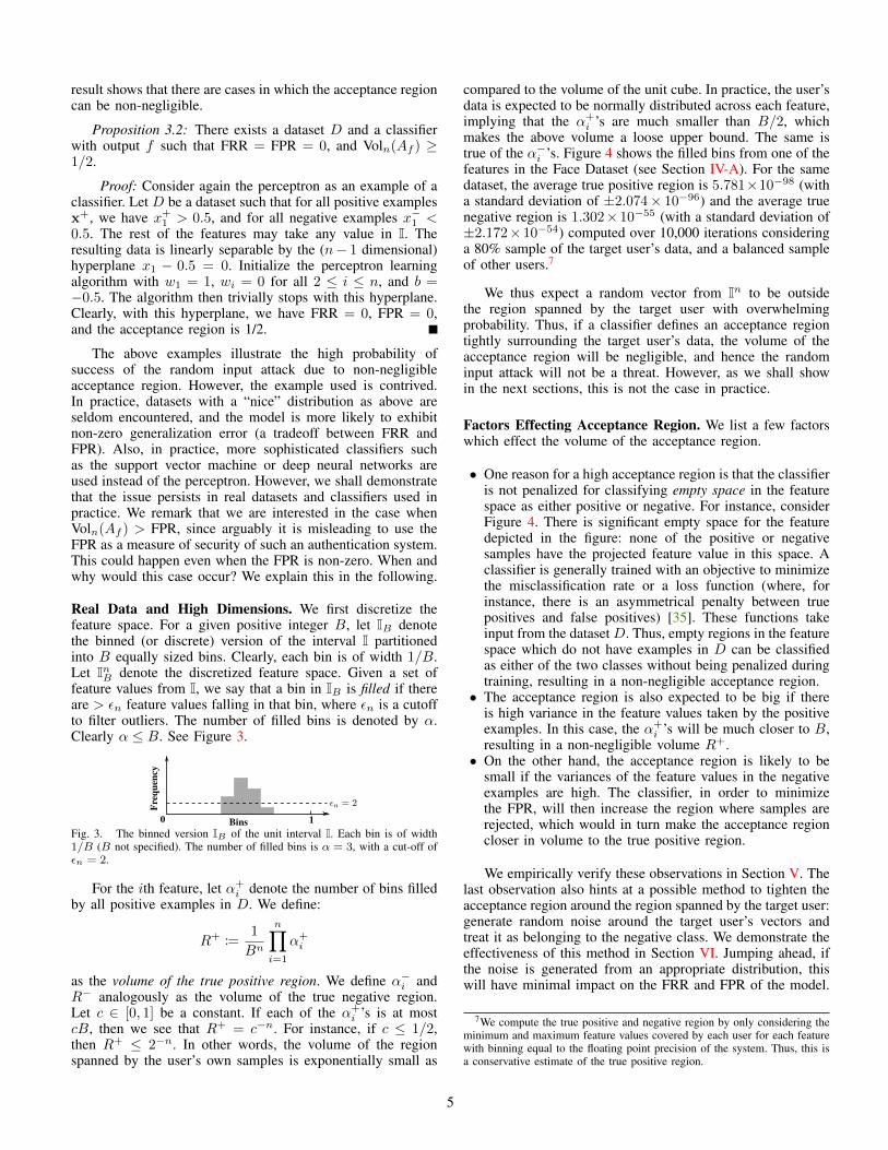
The above examples illustrate the high probability ofsuccess of the random input attack due to non-negligibleacceptance region. However, the example used is contrived.In practice, datasets with a “nice” distribution as above areseldom encountered, and the model is more likely to exhibitnon-zero generalization error (a tradeoff between FRR andFPR). Also, in practice, more sophisticated classifiers suchas the support vector machine or deep neural networks areused instead of the perceptron. However, we shall demonstratethat the issue persists in real datasets and classifiers used inpractice. We remark that we are interested in the case whenVoln(Af ) > FPR, since arguably it is misleading to use theFPR as a measure of security of such an authentication system.This could happen even when the FPR is non-zero. When andwhy would this case occur? We explain this in the following.
Real Data and High Dimensions. We first discretize thefeature space. For a given positive integer B, let IB denotethe binned (or discrete) version of the interval I partitionedinto B equally sized bins. Clearly, each bin is of width 1/B.Let InB denote the discretized feature space. Given a set offeature values from I, we say that a bin in IB is filled if thereare > εn feature values falling in that bin, where εn is a cutoffto filter outliers. The number of filled bins is denoted by α.Clearly α ≤ B. See Figure 3.
0 1
εn = 2Freq
uenc
y
BinsFig. 3. The binned version IB of the unit interval I. Each bin is of width1/B (B not specified). The number of filled bins is α = 3, with a cut-off ofεn = 2.
For the ith feature, let α+i denote the number of bins filled
by all positive examples in D. We define:
R+ :=1
Bn
n∏i=1
α+i
as the volume of the true positive region. We define α−i andR− analogously as the volume of the true negative region.Let c ∈ [0, 1] be a constant. If each of the α+
i ’s is at mostcB, then we see that R+ = c−n. For instance, if c ≤ 1/2,then R+ ≤ 2−n. In other words, the volume of the regionspanned by the user’s own samples is exponentially small as
compared to the volume of the unit cube. In practice, the user’sdata is expected to be normally distributed across each feature,implying that the α+
i ’s are much smaller than B/2, whichmakes the above volume a loose upper bound. The same istrue of the α−i ’s. Figure 4 shows the filled bins from one of thefeatures in the Face Dataset (see Section IV-A). For the samedataset, the average true positive region is 5.781×10−98 (witha standard deviation of ±2.074× 10−96) and the average truenegative region is 1.302×10−55 (with a standard deviation of±2.172×10−54) computed over 10,000 iterations consideringa 80% sample of the target user’s data, and a balanced sampleof other users.7
We thus expect a random vector from In to be outsidethe region spanned by the target user with overwhelmingprobability. Thus, if a classifier defines an acceptance regiontightly surrounding the target user’s data, the volume of theacceptance region will be negligible, and hence the randominput attack will not be a threat. However, as we shall showin the next sections, this is not the case in practice.
Factors Effecting Acceptance Region. We list a few factorswhich effect the volume of the acceptance region.
• One reason for a high acceptance region is that the classifieris not penalized for classifying empty space in the featurespace as either positive or negative. For instance, considerFigure 4. There is significant empty space for the featuredepicted in the figure: none of the positive or negativesamples have the projected feature value in this space. Aclassifier is generally trained with an objective to minimizethe misclassification rate or a loss function (where, forinstance, there is an asymmetrical penalty between truepositives and false positives) [35]. These functions takeinput from the dataset D. Thus, empty regions in the featurespace which do not have examples in D can be classifiedas either of the two classes without being penalized duringtraining, resulting in a non-negligible acceptance region.
• The acceptance region is also expected to be big if thereis high variance in the feature values taken by the positiveexamples. In this case, the α+
i ’s will be much closer to B,resulting in a non-negligible volume R+.
• On the other hand, the acceptance region is likely to besmall if the variances of the feature values in the negativeexamples are high. The classifier, in order to minimizethe FPR, will then increase the region where samples arerejected, which would in turn make the acceptance regioncloser in volume to the true positive region.
We empirically verify these observations in Section V. Thelast observation also hints at a possible method to tighten theacceptance region around the region spanned by the target user:generate random noise around the target user’s vectors andtreat it as belonging to the negative class. We demonstrate theeffectiveness of this method in Section VI. Jumping ahead, ifthe noise is generated from an appropriate distribution, thiswill have minimal impact on the FRR and FPR of the model.
7We compute the true positive and negative region by only considering theminimum and maximum feature values covered by each user for each featurewith binning equal to the floating point precision of the system. Thus, this isa conservative estimate of the true positive region.
5

0.0 0.2 0.4 0.6 0.8 1.0Value Bins
0
10
20
Freq
uenc
y εn = 2
Target UserOther Users
Fig. 4. The histogram of feature values of one of the features in the FaceDataset (cf. § IV-A). Here we have B = 100. The number of filled bins forthe target user is α+
i = 35 (with 400 samples), and for the negative class (10users; same number of total samples) it is α−
i = 50. A total of 24 bins arenot filled by any of the two classes, implying that (approximately) 0.24 ofthe region for this feature is empty.
IV. EVALUATION ON BIOMETRIC SYSTEMS
To evaluate the issue of acceptance region on real-worldbiometric systems, we chose four different modalities: gait,touch, face and voice. The last two modalities are used asexamples of user authentication at the point of entry into asecured system, whilst gait and touch are often used in con-tinuous authentication systems [37]. We first describe the fourbiometric datasets, followed by our evaluation methodology,the machine learning algorithms used, and finally our resultsand observations.
A. The Biometric Datasets
1) Activity Type (Gait) Dataset: The activity type dataset[38], which we will refer to as the “gait” dataset, was col-lected for human activity recognition. Specifically its aimis to provide a dataset for determining if a user is sitting,laying down, walking, running, walking upstairs or downstairs,etc. However, as the dataset retains the unique identifiersfor users per biometric record, we re-purpose the dataset forauthentication. This dataset contains 30 users, with an averageof 343± 35 (mean± SD) biometric samples per user, there isan equal number of activity type samples for each user. Forthe purpose of authentication, we do not isolate a specific typeof activity. Instead, we include them as values of an additionalfeature. The activity type feature increases the total number offeatures to 562. We will refer to these features as engineeredfeatures as they are manually defined (e.g., by an expert) asopposed to latent features extracted from a pre-trained neuralnetwork for the face and voice datasets.
2) Touch Dataset: The UMDAA-02 Touch Dataset [6] isa challenge dataset to provide data for researchers to performbaseline evaluations of new touch-based authentication sys-tems. Data was collected from 35 users, with an average of3667 ± 3012 swipes per user. This dataset was collected bylending mobile devices to the participants over a prolongedperiod of time. The uncontrolled nature of the collection pro-duces a dataset that accurately reflects swipe interactions withconstant and regular use of the device. This dataset containsevery touch interaction performed by the user including taps.In a pre-processing step we only consider sequences with morethan 5 data points as swipes. Additionally, we set four binaryfeatures to indicate the direction of the swipe, determined fromthe dominant vertical and horizontal displacement. We retainedall other features in [6] bar inter-stroke time, as we wished totreat each swipe independently, without chronological order.We substitute this feature with half-time of the stroke. Thisproduces a total of 27 engineered touch features.
3) Face Dataset: FaceNet [3] proposes a system based onneural networks that can effectively learn embeddings (featurevectors) that represent uniquely identifiable facial informationfrom images. Unlike engineered features, these embeddingsmay not be directly explainable as they are automaticallyextracted by the underlying neural network. This neural net-work can be trained from any dataset containing labeled facesof individuals. There are many sources from which we canobtain face datasets, CASIA-WebFace [2], VGGFace2 [39] andLabeled Faces in the Wild (LFW) [40] are examples of suchdatasets. However, with a pre-trained model, we can conservethe time and resources required to re-train the network. Thesource code for FaceNet [41] contains two pretrained modelsavailable for public use (at the time of writing): one trainedon CASIA-WebFace, and another trained on VGGFace2. Weopt to use a model pre-trained on VGGFace28 , while re-taining CASIA-WebFace as our dataset for classifier training.We choose to use different datasets for the training of theembeddings and the classifiers to simulate the exposure of themodel to never before seen data. Our face dataset is a subset ofCASIA-WebFace containing only the top 100 identities withthe largest number of face images (producing 447±103 imagesper individual). This model produces 512 latent features frominput images of pixel size 160x160 which have been centeredand aligned. Recall that face alignment involves finding abounding box on the face on an image, before cropping andresizing to the requested dimensions.
4) Speaker Verification (Utterances): VoxCeleb [4], andVoxCeleb2 [5] are corpuses of spoken recordings by celebritiesin online media. These recordings are text-independent, i.e.,the phrase uttered by the user is not pre-determined. Text-independent speaker verification schemes depart from text-dependent verification schemes in which the individual isbound to repeat a pre-determined speech content. Thus, thetask of text-independent verification (or identification) is todistinguish how the user speaks as an individual, instead ofhow the user utters a specific phrase. The former objectiveis an arguably harder task. Despite the increased difficulty,researchers have trained neural networks to convert speakerutterances into a set of latent features representing how indi-viduals speak. These works have also released their modelsto the public, increasing the accessibility of speaker verifi-cation to developers. We opt to use the pre-trained modelof VoxCeleb [4], with utterances from VoxCeleb2 [5]. FromVoxCeleb2, we only use the test portion of the dataset, whichcontains 118 Users with an average of 406 ± 87 utterances.VoxCeleb was trained as a Siamese neural network [42] forone-shot comparison between two audio samples. A Siamesenetwork consists of two identical branches that produce twoequal size outputs from two independent inputs for distancecomparison. To fit the pre-trained model into our evaluationof ML-based models, we extract embeddings from one of thetwin networks and disregard the second branch. The 1024-length embedding is then used as the feature vector within ourevaluation.
B. Evaluation Methodology
In our creation of biometric models for each user, we seekto obtain the baseline performance of the model with respect
8(20180402-114759) is the identifier of pre-trained model used.
6

to the ability of negative user samples gaining access (i.e.FPR), and the measured Acceptance Region (AR). We usethe following methodology to evaluate these metrics for eachdataset and each classification algorithm.
1) We min-max normalize each extracted feature over theentire dataset between 0 and 1.
2) We partition the dataset into a (70%, 30%) split for trainingand testing sets, respectively.
3) For both training and testing samples, we further samplean equal number of negative samples from every otheruser such that the total number of negative samples areapproximately equal to the number of samples from thetarget user, representing the positive class, i.e., the positiveand negative classes are balanced.
4) Using the balanced training set from step 3, we train a two-class classifier defining the target user set as the positiveclass, and all remaining users as negative.
5) We test the trained model using the balanced testing setfrom step 3. This establishes the FRR and FPR of thesystem.
6) We uniformly sample one million vectors from In, wheren is the dimension of the extracted features. Testing theset of vectors against the model measures the acceptanceregion (AR).
7) We record the confidence values of the test predictionfor the user’s positive test samples, other users’ negativetest samples, and the uniformly sampled vectors. Theseconfidence values produce ROC curves for FRR, FPR andAR.
8) Repeat steps 3-7 by iterating through every user in thedataset as the target user.
Remark 4.1: In general, the decision regions (accept andreject in the case of authentication) learned by the classifierscan be quite complex [43]. Hence, it is difficult to determinethem analytically, despite the availability of learned modelparameters. We instead use a Monte Carlo method by samplingrandom feature vectors from In where each feature value issampled uniformly at random from I. With enough samples(one million used in our experiments, and averaged over 50repetitions), the fraction of random samples accepted by theclassifier serves as an estimate of the acceptance region asdefined by Eq. 2 due to the law of large numbers.
Remark 4.2: Our evaluation of the biometric systems isusing the mock attacker model (samples from the negativeclass modelled as belonging to an attacker) as it is commonlyused [44]. We acknowledge that there are other attack modelssuch as excluding the data of the attacker from the trainingset [44]. Having the attacker data included in the trainingdataset, as in the mock attacker model, yields better EER. Onthe other hand, it is also likely to lower the AR of the system,due to increased variance in the negative training dataset. Thus,the use of this model does not inflate our results.
Remark 4.3: We have used balanced datasets in our ex-periments, i.e., the number of positive and negative samplesbeing the same. It is true that a balanced dataset is not idealfor minimizing AR; more negative samples may reduce theacceptance region. However, an unbalanced dataset, e.g., morenegative samples than positive samples, may be biased towardsthe negative class, resulting in misleadingly high accuracy [44],
[45]. A balanced dataset yields the best EER without beingbiased towards the positive or negative class.
C. Machine Learning Classifiers
Our initial hypothesis (Section III) stipulates that AR isrelated to the training data distribution, and not necessarilyto any weakness of the classifiers learning from the data. Todemonstrate this distinction, we elected four different machinelearning algorithms: Support Vector Machines (SVM) with alinear kernel (LinSVM), SVM with a radial basis functionkernel (RBFSVM), Random Forests (RNDF) and Deep NeuralNetworks (DNN). Briefly, SVM uses the training data toconstruct a decision boundary that maximizes the distancebetween the closest points of different classes (known assupport vectors). The shape of this boundary is dictated by thekernel used; we test both a linear and a radial kernel. RandomForests is an aggregation of multiple decision tree learnersformally known as an ensemble method. Multiple learnersin the aggregation are created through bagging, whereby thetraining dataset is split into multiple subsets, each subset train-ing a distinct decision tree. The decisions from the multiplemodels are then aggregated to produce the random forest’sfinal decision. DNNs are a class of machine learning modelsthat contain hidden layers between an input and an outputlayer; each layer containing neurons that activate as a functionof previous layers. Specifically we implement a convolutionalneural network with hidden layers leading to a final layer ofour two classes, accept and reject. All four of these machinelearning models are trained as supervised learners. As such, weprovide the ground truth labels to the model during training.
The linear SVM was trained with C = 104, and defaultvalues included within Scikit-learn’s Python library for theremaining parameters [46]. For radial SVM we also used C =104 while keeping the remaining parameters as default. TheRandom Forests classifier was configured with 100 estimators.DNNs were trained with TensorFlow Estimators [47] with avarying number of internal layers depending on the dataset.The exact configurations are noted in Appendix B.
Remark 4.4: We reiterate that our trained models arereconstructions of past works. However, we endeavor thatour models recreate error rates similar to the originally re-ported values on the same dataset. On Mahbub et al.’s touchdataset [6], the authors achieved 0.22 EER with a RNDFclassifier, by averaging 16 swipes for a single authenticationsession. We are able to achieve a comparable EER of 0.21on RNDF without averaging. For face authentication, weevaluate a subset of CASIA-Webface, consequently there is nodirect comparison. The original Facenet accuracy in verifyingpairs of LFW [40] faces is 98.87% [3], but our adoption ofmodel-based authentication is closer to [48], unfortunately theauthors have fixed a threshold for 0 FPR without reportingtheir TPR. Nagrani, Chung and Zisserman’s voice authenti-cator [4] reports an EER of 0.078 on a neural network. Ourclassifiers achieve EERs of 0.03, 0.02, 0.04 and 0.12, whichare within range of this benchmark. Our gait authenticatoris the exception, it has not been evaluated for authenticationwith it’s mixture of activity types. However, a review of gaitauthentication schemes can be found at [49].
7

0.0 0.2 0.4EER
0.00
0.25
0.50
0.75
1.00
AR
(a) Gait
0.0 0.2 0.4EER
0.00
0.25
0.50
0.75
1.00
AR
(b) Touch
0.0 0.2 0.4EER
0.00
0.25
0.50
0.75
1.00
AR
(c) Face
0.0 0.2 0.4EER
0.00
0.25
0.50
0.75
1.00
AR
LINSVMRBFSVMRNDFDNN
(d) VoiceFig. 5. Individual user scatter of AR and FPR. In a majority of configurations,there is no clear relationship between AR and FPR, with the exception of theRBFSVM and DNN classifiers for face and voice authentication.
D. Acceptance Region: Feature Vector API
In this section, we evaluate the acceptance region (AR)by comparing it against FPR for all 16 authentication config-urations (four datasets and four classifiers). In particular, wedisplay ROC curves showing the trade-off between FPR andFRR against the acceptance region (AR) curve as the modelthresholds are varied. These results are averaged over all users.While this gives an average picture of the disparity betweenAR and FPR, it does not highlight that for some users ARmay be substantially higher than FPR, and vice versa. In sucha case, the average AR might be misleading. Thus, we alsoshow scattered plots showing per-user AR and FPR, wherethe FPR is evaluated at EER. The per-user results have beenaveraged over 50 repetitions to remove any bias resulting fromthe sampled/generated vectors. The individual user AR versusFPR scatter plots are shown in Figure 5, and the (average) ARcurves against the ROC curves are shown in Figure 6.
Remark 4.5: EER is computed in a best effort manner,with only 100 discretized threshold values, to mitigate the stor-age demands of the 1M uniformly random vectors measuringAR. Unfortunately, there are some instances whereby the FRRand FPR do not match exactly, as the threshold step inducesa large change in both FRR and FPR. Only 1/16 classifiersexhibit an FPR-FRR discrepancy greater than 1%.
1) Gait Authentication: Figure 5a shows AR against FPRof every user in the activity type (gait) dataset. Recall that inthis figure FPR is evaluated at EER. The dotted straight line isthe line where AR equals FPR (or ERR). We note that there isa significant proportion of users for which AR is greater thanFPR, even when the latter is reasonably low. For instance, insome cases AR is close to 1.0 when the FPR is around 0.2.Thus, a random input attack on systems trained for these targetusers will be successful at a rate significantly higher than whatis suggested by FPR. We also note that the two SVM classifiershave higher instances of users for whom AR surpasses FPR.Figure 6a shows the AR curve averaged across all users againstthe FPR and FRR curves for all four classifiers. We can seethat AR is higher than the ERR (represented by the dottedvertical line) for the two SVM classifiers. For the remaining
two classifiers, AR is lower than EER. However, by lookingat the AR curve for RNDF, we see that the AR curve iswell above the FPR curve when FRR ≤ 0.3. This can bespecially problematic if the threshold is set so as to minimizefalse rejection at the expense of false positives. We also notethat the AR curve for DNN closely follows the FPR curve,which may suggest that the AR is not as problematic for thisclassifier. However, by looking at Figure 5a, we see that this ismisleading since for some users the AR is significantly higherthan FPR, making them vulnerable to random input attacks.Also, note that the AR generally decreases as the threshold ischanged at the expense of FRR. However, except for RNDF,the AR for the other three classifiers is significantly higherthan zero even for FRR values close to 1.
2) Touch (Swipe) Authentication: The touch authenticatorhas the highest EER of all four biometric modalities. Very fewusers attained an EER lower than 0.2 as seen in Figure 5b.This is mainly because we consider the setting where theclassification decision is being made after each input sample.Previous work has shown EER to improve if the decision ismade on an average vector of a few samples some work [28],[22], [8]. Nevertheless, since our focus is on AR, we stickto the per-sample decision setting. Figure 5b shows that morethan half of the users have ARs larger than FPR, and in somecases where the FPR is fairly low (say 0.2), the AR is higherthan 0.5. Unlike gait authentication where RNDF classifierhad ARs less than FPR for the majority of the users, all fouralgorithms for touch authentication display high vulnerabilityto the AR based random input attack. When viewing averageresults in Figure 6b, we observe the average AR curve to bevery ‘flat’ for both SVM classifiers and DNN. This indicatesthat AR for these classifier remains mostly unchanged evenif the threshold is moved closer to the extremes. RNDF onceagain is the exception, with the AR curve approaching 0 asthe threshold is increased.
3) Face Authentication: Figure 5c shows that AR is eitherlower or comparable to FPR for RBFSVM and DNN. Thus,the FPR serves as a good measure of AR in these systems.However, AR for most users is significantly higher than FPRfor LinSVM and RNDF. This is true even though the EERof these systems is comparable to the other two as seen inFigure 6c. For LINSVM, we have an average AR of 0.15compared to an EER of 0.05. For RNDF, the situation is worsewith the AR reaching 0.78 against an EER of 0.03. We alsonote that while the AR is equal to FPR for DNN, its value of0.10 is still worrisome to be resistant to random input attack.The relatively high FPR for DNN as compared to RBFSVM islikely due to a limited set of training data available in trainingthe neural network.
4) Voice Authentication: Figure 5d shows that once againLinSVM and RNDF have a significant proportion of users withAR higher than FPR, whereas for both RBFSVM and DNNthe AR of users is comparable to FPR. Looking at the averageARs in Figure 6d, we see that interestingly RNDF exhibits anaverage AR of 0.01 well below the ERR of 0.04. The averagesuppresses the fact that there is one user in the system with anAR close to 1.0 even with an EER of approximately 0.1, andtwo other users with an AR of 0.5 and 0.3 for which the EERis significantly below 0.1. Thus these specific users are moresusceptible to the random input attack. Only LinSVM has an
8

0.0 0.2 0.4 0.6 0.8 1.0LINSVM threshold
0.0
0.2
0.4
0.6
0.8
1.0
Erro
r
0.160.24
FRR - 0.16FPR - 0.16 AR - 0.24
0.0 0.2 0.4 0.6 0.8 1.0RBFSVM threshold
0.140.18
FRR - 0.14FPR - 0.14 AR - 0.18
0.0 0.2 0.4 0.6 0.8 1.0RNDF threshold
0.090.03
FRR - 0.09FPR - 0.09 AR - 0.03
0.0 0.2 0.4 0.6 0.8 1.0TFDNN threshold
0.240.20
FRR - 0.24FPR - 0.19 AR - 0.20
(a) Gait Average ROC
0.0 0.2 0.4 0.6 0.8 1.0LINSVM threshold
0.0
0.2
0.4
0.6
0.8
1.0
Erro
r
0.33
0.490.45
FRR - 0.33FPR - 0.32 AR - 0.49RAR - 0.45
0.0 0.2 0.4 0.6 0.8 1.0RBFSVM threshold
0.26
0.410.40
FRR - 0.26FPR - 0.27 AR - 0.41RAR - 0.40
0.0 0.2 0.4 0.6 0.8 1.0RNDF threshold
0.210.230.18
FRR - 0.21FPR - 0.21 AR - 0.23RAR - 0.18
0.0 0.2 0.4 0.6 0.8 1.0TFDNN threshold
0.330.300.32
FRR - 0.33FPR - 0.32 AR - 0.30RAR - 0.32
(b) Touch Average ROC
0.0 0.2 0.4 0.6 0.8 1.0LINSVM threshold
0.0
0.2
0.4
0.6
0.8
1.0
Erro
r
0.050.150.12
FRR - 0.05FPR - 0.05 AR - 0.15RAR - 0.12
0.0 0.2 0.4 0.6 0.8 1.0RBFSVM threshold
0.040.010.09
FRR - 0.04FPR - 0.04 AR - 0.01RAR - 0.09
0.0 0.2 0.4 0.6 0.8 1.0RNDF threshold
0.03
0.78
0.02
FRR - 0.03FPR - 0.03 AR - 0.78RAR - 0.02
0.0 0.2 0.4 0.6 0.8 1.0TFDNN threshold
0.090.100.10
FRR - 0.09FPR - 0.10 AR - 0.10RAR - 0.10
(c) Face Average ROC
0.0 0.2 0.4 0.6 0.8 1.0LINSVM threshold
0.0
0.2
0.4
0.6
0.8
1.0
Erro
r
0.030.08
FRR - 0.03FPR - 0.03 AR - 0.08
0.0 0.2 0.4 0.6 0.8 1.0RBFSVM threshold
0.020.00
FRR - 0.02FPR - 0.02 AR - 0.00
0.0 0.2 0.4 0.6 0.8 1.0RNDF threshold
0.040.01
FRR - 0.04FPR - 0.04 AR - 0.01
0.0 0.2 0.4 0.6 0.8 1.0TFDNN threshold
0.120.08
FRR - 0.12FPR - 0.11 AR - 0.08
(d) Voice Average ROC
Fig. 6. ROC curve versus the AR and RAR curves for all configurations. The EER is shown as a dotted vertical blue line. The FRR, FPR, AR and RARvalues shown in the legend are evaluated at EER (FPR = FRR). The RAR is only evaluated on the Touch and Face datasets.
9

average AR (0.08) higher than EER (0.03). The average ARof DNN is lower than EER (0.11), but it is still significantlyhigh (0.08). For RBFSVM we have an average AR close to 0.
Observations
In almost every configuration, we can observe that theaverage AR is either higher than the FPR or at best comparableto it. Furthermore, for some users the AR is higher thanFPR even though the average over all users may not reflectthis trend. This demonstrates that an attacker with no priorknowledge of the system can launch an attack against it viathe feature vector API. Moreover, for both the linear and radialSVM kernels, and some instances of the DNN classifier, weobserve a relatively flat AR curve as the threshold is varied,unlike the gradual convergence to 1 experienced by the FPRand FRR curves. These classifiers thus have a substantialacceptance region that accept samples as positives irrespectiveof the threshold. Random Forests is the only classifier wherethe AR curve shows significant drop as the threshold is varied.Random forests sub-divide the training dataset in a processcalled bagging, where each sub-division is used to train onetree within the forest. With different subsets of data, differenttraining data points will be closer to different empty regionsin feature space, thus producing varied predictions. Becausethe prediction confidence of RNDF is computed from theproportion of trees agreeing with a prediction, the lack ofconsensus within the ensemble of trees for the empty spacemay be the reason for the non-flat AR curve.
E. Acceptance Rate: Raw Input API
The results from the feature vector API are not necessarilyreflective of the success rate of a random input attack via theraw input API. One reason for this is that the feature vectorsextracted from raw inputs may or may not span the entirefeature space, and as a consequence the entire acceptanceregion. For this reason, we use the term raw acceptance rate(RAR) to evaluate the probability of successfully finding anaccepting sample via raw random inputs. To evaluate RAR,we select the touch and face biometric datasets. The raw inputof the touch authenticator is a time-series, whereas for the faceauthentication system it is an image.
1) Raw Touch Inputs: We used a continuous auto-regressive process (CAR) [50] to generate random timeseries.We opted for CAR due to the extremely high likelihood oftime-series values having a dependence on previous values.This time-series was then min-max scaled to approximatesensor bounds. For example the x-position has a maximumand minimum value of 1980 and 0 respectively, as dictatedby the number of pixels on a smartphone screen. Both theduration and length of the time-series were randomly sampledfrom reasonable bounds: 0.5 to 2.0 seconds and 30 to 200data-points, respectively. The time-series was subsequentlyparsed by the same feature extraction process as a legitimatetime-series, and the outputs scaled on a feature min-maxscale previously fit on real user data. In total we generate100,000 time-series, which are used to measure RAR over 50repetitions of the experiment.
The results of our experiments are shown in Figure 6b,with the curve labeled RAR showing the raw acceptance rate
as the threshold of each of the classifiers is changed. As wecan see, the RAR is large and comparable to AR. This seemsto indicate that the region spanned by random inputs coversthe acceptance region. However, on closer examination, thishappens to be false. The average volume covered by the truepositive region for the touch dataset (cf. Section III) is lessthan 1.289 × 10⁻⁴ ± 5.462 × 10⁻⁴, yet the volume occupiedby the feature vectors extracted from raw inputs is less than2.609×10−6. This is significantly smaller than the AR for allfour classifiers. We will return to this observation shortly.
2) Raw Face Inputs: We generated 100,000 images ofsize 160x160 pixels, with uniformly sampled RGB values.Feature embeddings were then extracted from the generatedimages with the pre-trained Facenet model (cf. Section IV-A3).This set of 100,000 raw input vectors, was parsed by a min-max scaler fitted to real user data. We did not align thenoisy images, as there is no facial information within theimage to align. Note that alignment is normally used in faceauthentication to detect facial boundaries within an image.Again, we aggregate results over 50 repetitions to remove anypotential biases.
The results from these raw inputs are shown in Figure 6c.We note that the RAR curve behaves much more similarly tothe FPR curve, than what was previously observed for rawtouch inputs. Also, in the particular example of RBFSVM,we obtain an RAR of 0.09 which is significantly higher thanthe AR (0.01) at the equal error rate. We again computed thetrue positive region and found that the average is 6.562 ×10−94 ± 6.521× 10−93. However, the volume covered by theraw inputs (after feature extraction) is only 4.670 × 10−390,which is negligible compared to the ARs (0.15, 0.01, 0.78 and0.10 for all four classifiers). Additional analysis shows thatonly one other user’s feature space overlapped with the spaceof raw inputs, with an overlapped area of 8.317×10−407, manyorders of magnitude smaller than both the positive users andthe raw feature space itself.
Observations
The threat of a random input attack via raw random inputsis also high, and in some cases greater than the FPR. However,the region spanned by the feature vectors from these raw inputsis exponentially small and hence does not span the acceptanceregion. Furthermore, the region also does not coincide with anytrue positive region. This implies that raw inputs may result inhigh raw acceptance rate due to the fact that the training datadoes not have representative vectors in the region spanned byraw inputs. We shall return to this observation when we discussmitigation strategies in Section VI.
V. SYNTHETIC DATASET
The analysis in the previous section was limited in thesense that we could not isolate the reasons behind the dis-crepancy between AR and FPR. Indeed, we saw that forsome configurations (dataset-classifier pairs), the AR curvenicely followed the FPR curve, e.g., the face dataset and DNN(Figure 5c), where as for others this was not the case. In orderto better understand the factors effecting AR, in this section weattempt to empirically verify the hypothesized factors effectingthe acceptance region outlined in Section III. Namely, high
10
-0.15 -0.1-0.05 0.0 0.05 0.1 0.15
LINSVM Relative Feature Variance
0.0
0.2
0.4
0.6
0.8
1.0Er
ror
-0.15 -0.1-0.05 0.0 0.05 0.1 0.15
RBFSVM Relative Feature Variance
0.0
0.2
0.4
0.6
0.8
1.0Overall FPROverall AROverall FRRIsolated FPRIsolated ARIsolated FRR
-0.15 -0.1-0.05 0.0 0.05 0.1 0.15
RNDF Relative Feature Variance
0.0
0.2
0.4
0.6
0.8
1.0
-0.15 -0.1-0.05 0.0 0.05 0.1 0.15
TFDNN Relative Feature Variance
0.0
0.2
0.4
0.6
0.8
1.0
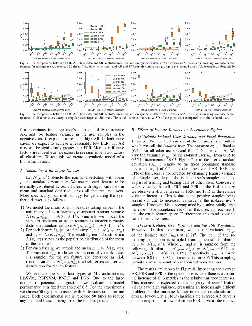
Fig. 7. A comparison between FPR, AR, four different ML architectures. Trained on synthetic data of 50 features of 50 user, of increasing variance withinfeatures for a singular user, repeated 50 times. Note how the system level AR and FPR remains unchanging, despite the isolated user’s AR increasing substantially.
-0.15 -0.1-0.05 0.0 0.05 0.1 0.15
LINSVM Relative Feature Variance
0.0
0.2
0.4
0.6
0.8
1.0
Erro
r
-0.15 -0.1-0.05 0.0 0.05 0.1 0.15
RBFSVM Relative Feature Variance
0.0
0.2
0.4
0.6
0.8
1.0Overall FPROverall AROverall FRRIsolated FPRIsolated ARIsolated FRR
-0.15 -0.1-0.05 0.0 0.05 0.1 0.15
RNDF Relative Feature Variance
0.0
0.2
0.4
0.6
0.8
1.0
-0.15 -0.1-0.05 0.0 0.05 0.1 0.15
TFDNN Relative Feature Variance
0.0
0.2
0.4
0.6
0.8
1.0
Fig. 8. A comparison between FPR, AR, four different ML architectures. Trained on synthetic data of 50 features of 50 user, of increasing variance withinfeatures of all other users except a singular user, repeated 50 times. The x-axis denotes the relative SD of the population compared with the isolated user.
feature variance in a target user’s samples is likely to increaseAR, and low feature variance in the user samples in thenegative class is expected to result in high AR. In both thesecases, we expect to achieve a reasonably low EER, but ARmay still be significantly greater than FPR. Moreover, if thesefactors are indeed true, we expect to see similar behavior acrossall classifiers. To test this we create a synthetic model of abiometric dataset.
A. Simulating a Biometric Dataset
Let N (µ, σ2), denote the normal distribution with meanµ and standard deviation σ. We assume each feature to benormally distributed across all users with slight variations inmean and standard deviation across all features and users.More specifically, our methodology for generating the syn-thetic dataset is as follows.
1) We model the mean of all n features taking values in theunit interval I as a normally distributed random variableN (µmn, σ
2mn) = N (0.5, 0.12). Similarly we model the
standard deviation of all n features as another normallydistributed random variable N (µvar, σ
2var) = N (0.1, 0.072).
2) For each feature i ∈ [n], we first sample µi ← N (µmn, σ2mn)
and σi ← N (µvar, σ2var). The resulting normal distribution
N (µi, σ2i ) serves as the population distribution of the mean
of the feature i.3) For each user u, we sample the mean µu,i ← N (µi, σ
2i ).
The variance σ2u,i is chosen as the control variable. User
u’s samples for the ith feature are generated as i.i.d.random variables N (µu,i, σ
2u,i), which serves as user u’s
distribution for the ith feature.
We evaluate the same four types of ML architectures,LinSVM, RBFSVM, RNDF and DNN. Due to the largenumber of potential configurations we evaluate the modelperformance at a fixed threshold of 0.5. For the experimentswe choose 50 (synthetic) users, with 50 features in the featurespace. Each experimental run is repeated 50 times to reduceany potential biases arising from the random process.
B. Effects of Feature Variance on Acceptance Region
1) Variable Isolated User Variance and Fixed PopulationVariance: We first treat one out of the 50 users as an outlier,whcih we call the isolated user. The variance σ2
u,i is fixed at(0.2)2 for all other users u and for all features i ∈ [n]. Wevary the variance σutgt,i of the isolated user utgt from 0.05 to0.35 in increments of 0.05. Figure 7 plots the user’s standarddeviation (σutgt,i) relative to the fixed population standarddeviation (σu,i) of 0.2. It is clear the overall AR, FRR andFPR of the users is not affected by changing feature varianceof a single user, despite the isolated user’s samples includedas part of training and testing data of other users. Conversely,when viewing the AR, FRR and FPR of the isolated user,we observe a slight increase in FRR and FPR as the relativevariance increases. This is due to the positive samples beingspread out due to increased variance in the isolated user’ssamples. However, this is accompanied by a substantially largeincrease in the acceptance region of this user, approaching 1,i.e., the entire feature space. Furthermore, this trend is visiblefor all four classifiers.
2) Fixed Isolated User Variance and Variable PopulationVariance: In this experiment, we fix the variance σ2
utgt,i
of the isolated user (utgt) at (0.2)2. The σ2u,i of the re-
maining population is sampled from a normal distributionσu,i ← N (µi, σ
2i ). Where µi and σi is sampled from the
following distributions N (µmn, σ2mn) = N (µmn, 0.05
2) andN (µvar, σ
2var) = N (0.03, 0.022), respectively. µmn is varied
between 0.05 and 0.35 in increments on 0.05 This samplingpermits a small amount of variation between features.
The results are shown in Figure 8. Inspecting the averageAR, FRR and FPR of the system, it is evident there is a contin-ual increase of all 3 metrics as the relative variance increases.This increase is expected as the majority of users’ featurevalues have high variance, presenting an increasingly difficultproblem for the machine learner to reduce misclassificationerrors. However, in all four classifiers the average AR curve iseither comparable or lower than the FPR curve as the relative
11

0.0 0.2 0.4 0.6 0.8 1.0Linear SVM threshold
0.0
0.2
0.4
0.6
0.8
1.0Er
ror
0.000.08
FRR - 0.00FPR - 0.00 AR - 0.08
0.0 0.2 0.4 0.6 0.8 1.0Radial SVM threshold
0.000.05
FRR - 0.00FPR - 0.00 AR - 0.05
0.0 0.2 0.4 0.6 0.8 1.0Random Forests threshold
0.000.01
FRR - 0.00FPR - 0.00 AR - 0.01
0.0 0.2 0.4 0.6 0.8 1.0Cosine Similarity threshold
0.110.00
FRR - 0.11FPR - 0.11 AR - 0.00
Fig. 9. ROC Curves versus the AR curve for different ML architectures, including a cosine similarity distance-based classifier. Trained on synthetic data of 50features of 50 user, with fixed mean and variance for features of all users, repeated 50 times.
25 50 75 100 125 150LINSVM Number of Users
0.000
0.025
0.050
0.075
0.100
0.125
Erro
r
25 50 75 100 125 150RBFSVM Number of Users
0.000
0.025
0.050
0.075
0.100
0.125
25 50 75 100 125 150RNDF Number of Users
0.000
0.025
0.050
0.075
0.100
0.125 MetricFPRARFRR
25 50 75 100 125 150TFDNN Number of Users
0.000
0.025
0.050
0.075
0.100
0.125
Fig. 10. A comparison between FPR and AR of four different ML architectures. Trained on synthetic data of 50 features per user, with a variable number ofusers, repeated 50 times.
variance increases. For the isolated user, we see that when therelative variance of all other users is lower than this user (to theleft), the AR is significantly higher even though the FPR andFRR are minimal in all four classifiers. This shows that lessvariance in the population samples will result in a high AR,as the classifier need not tighten AR around the true positiveregion, due to lack of high variance negative samples. On theother hand, AR of the isolated user decreases as the relativevariance of the population increases.
C. On Distance Based Classifiers
As noted earlier, it has been stated that random in-puts are ineffective against distance-based classification al-gorithms [17]. This is in contrast to the machine learningbased algorithms evaluated in this paper. We take a briefinterlude to experimentally evaluate this claim on the cosinesimilarity distance-based classifier. We sample 50 featureswith means distributed as N (µmn, σ
2mn) = N (0.2, 0.052) and
variance distributed as N (µvar, σ2var) = N (0.03, 0.022). Cosine
similarity is computed between two vectors of the samelength. As our positive training data contains more than onetraining sample, we use the average of these samples as therepresentative template of the user [29]. We use a fixed numberof 50 users, with the experiment repeated 50 times. Recallthat our evaluation at each threshold is best-effort; we use1,000 threshold bins for the evaluation of the cosine similarityclassifier, since the FRR and FPR rapidly change over a smallrange of thresholds.
Figure 9 displays three classical machine learning al-gorithms of linear SVM, radial SVM, and random forests,alongside a distance-based cosine similarity classifier. It isclear from the figure, that the AR is near zero for cosinesimilarity, unlike the other classifiers using the same syntheticdataset. This, however, comes at the cost of higher EER.This suggests that distance-based classifiers are effective in
minimizing the AR of model, but at the expense of accuracyof the system. We leave further investigation of distance-basedclassifiers as future work.
D. Effects of Increasing Synthetic Users
The real-world datasets used in Section IV have a variablenumber of users. Our binary classification task aggregatesnegative user samples into a negative class, resulting in dis-tributions and variances of the negative class which dependon the number of users in the datasets. Thus, in this test weinvestigate the impact on TPR, FPR and AR by varying thenumber of users in the dataset. We use the synthetic datasetconfigured in the same manner as in Section V-C. We increasethe number of users within the synthetic dataset, from 25 to150, in increments of 25. Note that the split between positiveand negative samples is still balanced (see Remark 4.3).
In Figure 10, we observe that with the addition of moreusers, there is a slight increase in the FPR. This is expected asthe likelihood of user features being similar between any twousers will increase with more users in the population. As thetraining of the classifier uses samples from other users as anegative class, the increased number of negative users slightlylowers the AR of the classifier, with an increased variation ofthe negative training set (from additional users) covering moreof the feature space. However, both these changes are relativelyminor despite the multi-fold increase in the number of users.Thus, the AR of the classifiers remains relatively stable withan increasing number of users.
VI. MITIGATION
In the previous section, we validated that higher variance inthe samples in the negative class as compared to the varianceof samples from the target user class reduces AR. The datafrom the negative class is obtained from real user samples,and therefore scheme designers cannot control the variance.
12
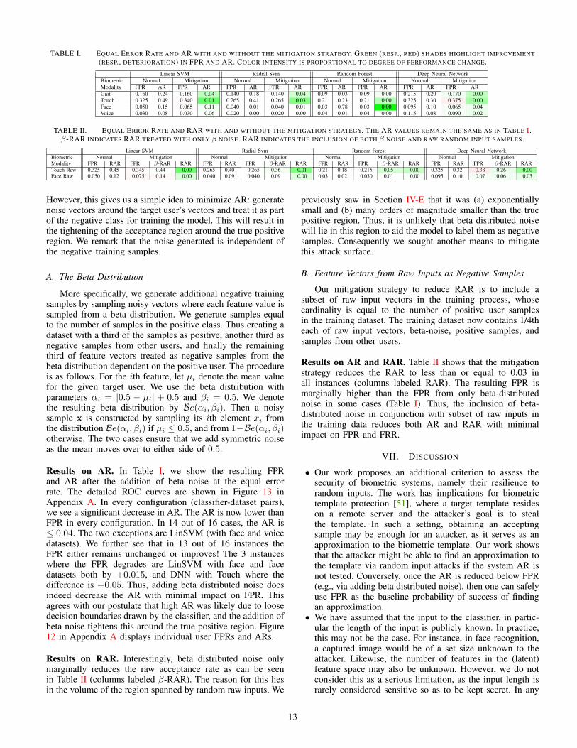
TABLE I. EQUAL ERROR RATE AND AR WITH AND WITHOUT THE MITIGATION STRATEGY. GREEN (RESP., RED) SHADES HIGHLIGHT IMPROVEMENT(RESP., DETERIORATION) IN FPR AND AR. COLOR INTENSITY IS PROPORTIONAL TO DEGREE OF PERFORMANCE CHANGE.
Linear SVM Radial Svm Random Forest Deep Neural NetworkBiometric Normal Mitigation Normal Mitigation Normal Mitigation Normal MitigationModality FPR AR FPR AR FPR AR FPR AR FPR AR FPR AR FPR AR FPR ARGait 0.160 0.24 0.160 0.04 0.140 0.18 0.140 0.04 0.09 0.03 0.09 0.00 0.215 0.20 0.170 0.00Touch 0.325 0.49 0.340 0.01 0.265 0.41 0.265 0.03 0.21 0.23 0.21 0.00 0.325 0.30 0.375 0.00Face 0.050 0.15 0.065 0.11 0.040 0.01 0.040 0.01 0.03 0.78 0.03 0.00 0.095 0.10 0.065 0.04Voice 0.030 0.08 0.030 0.06 0.020 0.00 0.020 0.00 0.04 0.01 0.04 0.00 0.115 0.08 0.090 0.02
TABLE II. EQUAL ERROR RATE AND RAR WITH AND WITHOUT THE MITIGATION STRATEGY. THE AR VALUES REMAIN THE SAME AS IN TABLE I.β-RAR INDICATES RAR TREATED WITH ONLY β NOISE. RAR INDICATES THE INCLUSION OF BOTH β NOISE AND RAW RANDOM INPUT SAMPLES.
Linear SVM Radial Svm Random Forest Deep Neural NetworkBiometric Normal Mitigation Normal Mitigation Normal Mitigation Normal MitigationModality FPR RAR FPR β-RAR RAR FPR RAR FPR β-RAR RAR FPR RAR FPR β-RAR RAR FPR RAR FPR β-RAR RARTouch Raw 0.325 0.45 0.345 0.44 0.00 0.265 0.40 0.265 0.36 0.01 0.21 0.18 0.215 0.05 0.00 0.325 0.32 0.38 0.26 0.00Face Raw 0.050 0.12 0.075 0.14 0.00 0.040 0.09 0.040 0.09 0.00 0.03 0.02 0.030 0.01 0.00 0.095 0.10 0.07 0.06 0.03
However, this gives us a simple idea to minimize AR: generatenoise vectors around the target user’s vectors and treat it as partof the negative class for training the model. This will result inthe tightening of the acceptance region around the true positiveregion. We remark that the noise generated is independent ofthe negative training samples.
A. The Beta Distribution
More specifically, we generate additional negative trainingsamples by sampling noisy vectors where each feature value issampled from a beta distribution. We generate samples equalto the number of samples in the positive class. Thus creating adataset with a third of the samples as positive, another third asnegative samples from other users, and finally the remainingthird of feature vectors treated as negative samples from thebeta distribution dependent on the positive user. The procedureis as follows. For the ith feature, let µi denote the mean valuefor the given target user. We use the beta distribution withparameters αi = |0.5 − µi| + 0.5 and βi = 0.5. We denotethe resulting beta distribution by Be(αi, βi). Then a noisysample x is constructed by sampling its ith element xi fromthe distribution Be(αi, βi) if µi ≤ 0.5, and from 1−Be(αi, βi)otherwise. The two cases ensure that we add symmetric noiseas the mean moves over to either side of 0.5.
Results on AR. In Table I, we show the resulting FPRand AR after the addition of beta noise at the equal errorrate. The detailed ROC curves are shown in Figure 13 inAppendix A. In every configuration (classifier-dataset pairs),we see a significant decrease in AR. The AR is now lower thanFPR in every configuration. In 14 out of 16 cases, the AR is≤ 0.04. The two exceptions are LinSVM (with face and voicedatasets). We further see that in 13 out of 16 instances theFPR either remains unchanged or improves! The 3 instanceswhere the FPR degrades are LinSVM with face and facedatasets both by +0.015, and DNN with Touch where thedifference is +0.05. Thus, adding beta distributed noise doesindeed decrease the AR with minimal impact on FPR. Thisagrees with our postulate that high AR was likely due to loosedecision boundaries drawn by the classifier, and the addition ofbeta noise tightens this around the true positive region. Figure12 in Appendix A displays individual user FPRs and ARs.
Results on RAR. Interestingly, beta distributed noise onlymarginally reduces the raw acceptance rate as can be seenin Table II (columns labeled β-RAR). The reason for this liesin the volume of the region spanned by random raw inputs. We
previously saw in Section IV-E that it was (a) exponentiallysmall and (b) many orders of magnitude smaller than the truepositive region. Thus, it is unlikely that beta distributed noisewill lie in this region to aid the model to label them as negativesamples. Consequently we sought another means to mitigatethis attack surface.
B. Feature Vectors from Raw Inputs as Negative Samples
Our mitigation strategy to reduce RAR is to include asubset of raw input vectors in the training process, whosecardinality is equal to the number of positive user samplesin the training dataset. The training dataset now contains 1/4theach of raw input vectors, beta-noise, positive samples, andsamples from other users.
Results on AR and RAR. Table II shows that the mitigationstrategy reduces the RAR to less than or equal to 0.03 inall instances (columns labeled RAR). The resulting FPR ismarginally higher than the FPR from only beta-distributednoise in some cases (Table I). Thus, the inclusion of beta-distributed noise in conjunction with subset of raw inputs inthe training data reduces both AR and RAR with minimalimpact on FPR and FRR.
VII. DISCUSSION
• Our work proposes an additional criterion to assess thesecurity of biometric systems, namely their resilience torandom inputs. The work has implications for biometrictemplate protection [51], where a target template resideson a remote server and the attacker’s goal is to stealthe template. In such a setting, obtaining an acceptingsample may be enough for an attacker, as it serves as anapproximation to the biometric template. Our work showsthat the attacker might be able to find an approximation tothe template via random input attacks if the system AR isnot tested. Conversely, once the AR is reduced below FPR(e.g., via adding beta distributed noise), then one can safelyuse FPR as the baseline probability of success of findingan approximation.• We have assumed that the input to the classifier, in partic-
ular the length of the input is publicly known. In practice,this may not be the case. For instance, in face recognition,a captured image would be of a set size unknown to theattacker. Likewise, the number of features in the (latent)feature space may also be unknown. However, we do notconsider this as a serious limitation, as the input length israrely considered sensitive so as to be kept secret. In any
13

case, the security of the system should not be reliant onkeeping this information secret following Kerckhoffs’s wellknown principle.
• We note that there are various detection mechanisms thatprotect the front-end of biometric systems. For example,spoofing detection [52] is an active area in detectingspeaker style transfer [53]. Detection of replay attacks isalso leveraged to ensure the raw captured biometric isnot reused, for example audio recordings [54]. There isalso liveliness detection, which seeks to determine if thebiometric that is presented is characteristic of a real personand not a recreation, e.g., face masks remain relativelystatic and unmoving compared to a real face [55]. Our at-tack surface applies once the front-end has been bypassed.Our mitigation measures can thus be used in conjunctionwith these detection mechanisms to thwart random inputattacks. Being generic, our mitigation measures also workfor systems which do not have defense measures similar toliveness detection.
• Once an accepting sample via the feature vector APIhas been found, it may be possible to obtain an inputthat results in this sample (after feature extraction), asdemonstrated by Garcia et al. with the training of an auto-encoder for both feature extraction and the regeneration ofthe input image [23].
• In this work, we have focused on authentication as a binaryclassification problem, largely because of its widespreaduse in biometric authentication [8], [9], [10], [11], [12],[13], [14], [15], [16], [26]. However, authentication has alsobeen framed as a one-class classification problem [56], [26]or as multi-class classification [26], e.g., in a discriminationmodel, as noted earlier. In one-class classification, onlysamples from the target user are used to create the template,and the goal is to detect outliers. If this is achieved in amanner similar to distance-based classifiers, then as wehave seen in Section V-C, and as previously indicatedin [17], the AR is expected to be small. In the multi-classsetting, each of the n users is treated as a different class.This increase in classes is expected to proportionally lowerthe AR. However, whether this behavior is observed on realworld data requires additional experimentation. We remarkthat as observed in Section V-B, AR is highly dependent onthe relative variance of the positive user and the negativeuser features. This may lead to the possibility of larger ARfor some of the users, consequently leading to higher riskof attack for these users. We leave thorough investigationof the one-class and multi-class settings as future work.
VIII. RELATED WORK
There are several mentions of attacks similar to the randominput attack discussed in this paper. Pagnin et al. [17] definea blind brute-force attack on biometric systems where the at-tacker submits random inputs to find an accepting sample. Theinputs are n-element vectors whose elements are integers in theset {0, 1, . . . , q−1}. The authors conclude that the probabilityof success of this attack is exponential in n, assuming thatthe authentication is done via a distance function (discardingany vector outside the ball of radius determined by the systemthreshold). They concluded that blind brute force attack is noteffective in recovering an accepting sample. While this mayapply to distance-based matching, the same conclusion cannot
be made about machine learning based algorithms whosedecision functions are more involved. Indeed, we have shownthat the acceptance region for machine learning classifiers isnot exponentially small. It has also been argued that the successrate of random input attacks can be determined by the falsepositive rate (FPR), at least in the case of fingerprint and faceauthentication [18], [19]. We have shown that for sophisticatedmachine learning classifiers this conclusion is not true, andrandom input attacks in many instances success at a rate higherthan FPR. A more involved method is hill-climbing [57], [18]which seeks an accepting sample via exploiting the confidencescores returned by the matching algorithm. The authenticationsystems considered in this paper do not return confidencescores.
Serwadda and Phoha [58] use a robotic finger and popu-lation statistics of touch behavior on smartphones to launcha physical attack on touch-based biometric authenticationsystems. Their attack reduces the accuracy of the system byincreasing the EER. In contrast, our work does not assume anyknowledge of population biometric statistics, e.g., populationdistribution of feature space. It is an interesting area of workto investigate whether a robotic finger can be programmed togenerate raw inputs used in our attack.
Garcia et al. [23] use explainable-AI techniques [48] toconstruct queries (feature vectors) to find an accepting samplein machine learning based biometric authentication systems.On a system with 0 FPR, they show that their attack issuccessful in breaching the system with up to 93% successrate. However, their attack is more involved: it requires theconstruction of a seed dataset containing representative ac-cepting and rejecting samples of a user set chosen by theadversary. This dataset trains a neural network as a substituteto the classifier of the authentication system. The adversarythen uses explainable AI techniques to obtain an acceptingsample of a target user (not in the seed dataset) in as fewqueries as possible, by updating the substitute network. Theauthors also report a random feature vector attack, however, theattack is only successful on one out of 16 victims. The randomfeature vector is constructed by sampling each feature valuevia a normal distribution (distribution parameters not stated),unlike the uniform distribution in our case. We also note thatthey propose including images with randomly perturbed pixelsas a counter-measure to defend against the aforementionedrandom input attack. This is different from our proposed beta-distributed noise mitigation technique, as it is agnostic to theunderlying biometric modality.
The frog-boiling attack [59], [60] studies the impact ofgradual variations in training data samples to manipulate theclassifier decision boundary. In this work we do not considerthe adversary with access to the training process, nor do weevaluate models with an iterative update process. If this threatmodel is considered for the problem addressed in this paper,then an adversary may seek to maximize the acceptance regionof a model by gradually poisoning the training dataset. As wehave demonstrated in Section V, the relative variance betweenthe user’s data and population dataset directly impacts AR.Thus the manipulation of a user’s training samples to be morevaried would be effective in increasing the AR. Likewise, inour mitigation technique, we have shown that beta-distributednoise is effective in the minimization of AR. However an
14

adversary might poison the training data by labeling betanoise as positive samples resulting in a maximization of theacceptance region to near 100% of the feature space.
Our work is different from another line of work thattargets machine learning models in general. For instance, thework in [61] shows an evasion attack where the adversary,through only blackbox access to a neural network, forces theclassifier to misclassify an input by slightly perturbing theinput even though the perturbed sample is perceptually similarto the original sample, e.g., noisy images. The attack can beapplicable to the authentication setting as well. However, itrelies on the confidence values (probability vectors) returnedby the classifier, which is not the case in authentication.Similarly, the work in [62] shows how to steal a machinelearning model, i.e., retrieve its undisclosed parameters, whichonly returns class labels (accept/reject decision in the case ofauthentication). They describe several techniques including theLowd and Meek attack [63] to retrieve a model sufficientlysimilar to the target model. The machine learning modelsconsidered in their attack are for applications different fromauthentication where one expects to find an accepting samplewith negligible probability.
There are also proposals to defend against the above men-tioned evasion attacks. The goal is to make the classifiers ro-bust against adversarial inputs in the sense that classification isconstant within a ball of certain radius around each input [64],[65]. Madry et al. [64] propose a theoretical framework whichformalizes defense against adversarial attacks by includingadversarially perturbed samples in the loss function of DNNs.They show that it is possible to train DNNs robust against awide range of adversarial input attacks. Cao and Gong [66]propose another defense where given a test input, randompoints within a hypercube surrounding the input are sampled,and the majority label returned by the already trained DNN isassigned to the test input. Randomized smoothing [65] createsa separate classifier from any classifier such that its predictionwithin a Gaussian noise region (ball) around any input isconstant, and consequently less likely to produce an erroneousprediction. We note that in evasion attacks there is a notion ofnearness, i.e., the adversary is given an input and seeks to adda small amount of noise such that the resultant erroneouslylabelled input is close to the original input. In contrast, in ourcase the random input need not be close to the target user’ssamples or even follow the same distribution. Furthermore,we have shown that even a conservative estimate of the truepositive region is negligible in comparison to the entirety ofthe feature space (Section III-B). Thus, it is unclear whethersuch defenses apply to uniform random inputs, as opposed torandom perturbations of inputs.
Membership inference attacks [24], [25] attempt to de-termine if a record obtained by an adversary was part ofthe original training data of the model. Whilst this attackdoes not compromise the security of the model, it breachesthe privacy of the individual records. These attacks createa shadow model [24] to mimic the behavior of the targetmodel. Salem et al. [25] construct a shadow model usingonly positive class samples and negative noise generated viauniformly random feature vectors. However it is hypothesizedthat these random samples belong to non-members, i.e., thenegative class [25, §V.B]. We have shown that a large portion
of these random inputs may also belong to the positive class.
Finally, we point to other works in literature analyzingthe security of biometric authentication systems. Sugrim etal. [45] survey and evaluate a range of performance met-rics used in biometric authentication schemes. They seekto motivate scheme designers to leverage robust metrics toprovide a complete description of the system, including aproposal of the new metric: Frequency Count Score (FCS). TheFCS metric shows a distribution of scores of legitimate andunauthorized users, identifying the overlap between the twodistributions which helps to select the appropriate thresholdfor the classification decision. The FCS, however, is dependenton the negative class or samples of other users, which doesnot include random inputs. The work in [67] investigatesthe accuracy of authentication systems reported on a smallnumber of participants when evaluated over an increasingnumber of users. The authors suggest that performance limitsof a system with a small number of participants should beevaluated iteratively by increasing the participant count untila the performance degrades below a tolerable limit.
IX. CONCLUSION
It is important to assess the security of biometric au-thentication systems against random input attacks akin tothe security of passwords against random guess attacks. Wehave demonstrated that without intentionally including randominputs as part of the training process of the underlying machinelearning algorithm, the authentication system is likely to besusceptible to random input attacks at a rate higher thanindicated by EER. Absent any other detection mechanism, e.g.,liveliness detection, this renders the system vulnerable. Themitigation measures proposed in this paper can be adopted todefend against such attacks.
X. ACKNOWLEDGMENTS
This research was funded by the Optus Macquarie Uni-versity Cybersecurity Hub, Data61 CSIRO and an AustralianGovernment Research Training Program (RTP) Scholarship.We would like to thank the anonymous reviewers and ourshepherd Kevin Butler for their feedback to improve the paper.
REFERENCES
[1] D. Maltoni, D. Maio, A. K. Jain, and S. Prabhakar, Handbook offingerprint recognition. Springer Science & Business Media, 2009.
[2] D. Yi, Z. Lei, S. Liao, and S. Z. Li, “Learning face representation fromscratch,” arXiv preprint arXiv:1411.7923, 2014.
[3] F. Schroff, D. Kalenichenko, and J. Philbin, “Facenet: A unifiedembedding for face recognition and clustering,” in Proceedings of theIEEE conference on computer vision and pattern recognition, 2015.
[4] A. Nagrani, J. S. Chung, and A. Zisserman, “Voxceleb: a large-scalespeaker identification dataset,” arXiv preprint arXiv:1706.08612, 2017.
[5] J. S. Chung, A. Nagrani, and A. Zisserman, “Voxceleb2: Deep speakerrecognition,” arXiv preprint arXiv:1806.05622, 2018.
[6] U. Mahbub, S. Sarkar, V. M. Patel, and R. Chellappa, “Active userauthentication for smartphones: A challenge data set and benchmarkresults,” in Biometrics Theory, Applications and Systems (BTAS), 2016IEEE 8th International Conference on. IEEE, 2016, pp. 1–8.
[7] W. Xu, G. Lan, Q. Lin, S. Khalifa, N. Bergmann, M. Hassan, and W. Hu,“Keh-gait: Towards a mobile healthcare user authentication system bykinetic energy harvesting.” in NDSS, 2017.
15

0.0 0.2 0.4 0.6 0.8 1.0LINSVM threshold
0.0
0.2
0.4
0.6
0.8
1.0
Erro
r
0.36
0.010.00
FRR - 0.36FPR - 0.33 AR - 0.01RAR - 0.00
0.0 0.2 0.4 0.6 0.8 1.0RBFSVM threshold
0.27
0.030.01
FRR - 0.27FPR - 0.26 AR - 0.03RAR - 0.01
0.0 0.2 0.4 0.6 0.8 1.0RNDF threshold
0.21
0.000.00
FRR - 0.21FPR - 0.22 AR - 0.00RAR - 0.00
0.0 0.2 0.4 0.6 0.8 1.0TFDNN threshold
0.38
0.020.00
FRR - 0.38FPR - 0.38 AR - 0.02RAR - 0.00
(a) Touch Average ROC in the presence of Beta Noise
0.0 0.2 0.4 0.6 0.8 1.0LINSVM threshold
0.0
0.2
0.4
0.6
0.8
1.0
Erro
r
0.080.110.00
FRR - 0.08FPR - 0.07 AR - 0.11RAR - 0.00
0.0 0.2 0.4 0.6 0.8 1.0RBFSVM threshold
0.040.010.00
FRR - 0.04FPR - 0.04 AR - 0.01RAR - 0.00
0.0 0.2 0.4 0.6 0.8 1.0RNDF threshold
0.030.000.00
FRR - 0.03FPR - 0.03 AR - 0.00RAR - 0.00
0.0 0.2 0.4 0.6 0.8 1.0TFDNN threshold
0.060.050.03
FRR - 0.06FPR - 0.07 AR - 0.05RAR - 0.03
(b) Face Average ROC in the presence of Beta NoiseFig. 11. Beta-noise mitigation of AR, with additional negative samples from the RAR feature set. The EER is marked on the diagrams as a vertical line.Addition RAR vectors were included as it was previously observed that beta noise is sufficient in mitigating AR attacks, but not the RAR attack.
[8] J. Chauhan, B. Z. H. Zhao, H. J. Asghar, J. Chan, and M. A. Kaafar,“Behaviocog: An observation resistant authentication scheme,” in In-ternational Conference on Financial Cryptography and Data Security.Springer, 2017, pp. 39–58.
[9] M. T. Curran, N. Merrill, J. Chuang, and S. Gandhi, “One-step, three-factor authentication in a single earpiece,” in Proceedings of the 2017ACM International Joint Conference on Pervasive and UbiquitousComputing and Proceedings of the 2017 ACM International Symposiumon Wearable Computers. ACM, 2017, pp. 21–24.
[10] C. Huang, H. Chen, L. Yang, and Q. Zhang, “Breathlive: Liveness detec-tion for heart sound authentication with deep breathing,” Proceedings ofthe ACM on Interactive, Mobile, Wearable and Ubiquitous Technologies,vol. 2, no. 1, p. 12, 2018.
[11] R. Liu, C. Cornelius, R. Rawassizadeh, R. Peterson, and D. Kotz, “Vocalresonance: Using internal body voice for wearable authentication,” Pro-ceedings of the ACM on Interactive, Mobile, Wearable and UbiquitousTechnologies, vol. 2, no. 1, p. 19, 2018.
[12] Y. Chen, J. Sun, X. Jin, T. Li, R. Zhang, and Y. Zhang, “Your face yourheart: Secure mobile face authentication with photoplethysmograms,”in IEEE INFOCOM 2017-IEEE Conference on Computer Communica-tions. IEEE, 2017, pp. 1–9.
[13] C. Song, A. Wang, K. Ren, and W. Xu, “Eyeveri: A secure and usableapproach for smartphone user authentication,” in IEEE INFOCOM2016-The 35th Annual IEEE International Conference on ComputerCommunications. IEEE, 2016, pp. 1–9.
[14] J. Chauhan, Y. Hu, S. Seneviratne, A. Misra, A. Seneviratne, andY. Lee, “Breathprint: Breathing acoustics-based user authentication,”in Proceedings of the 15th Annual International Conference on MobileSystems, Applications, and Services. ACM, 2017, pp. 278–291.
[15] J. Ho and D.-K. Kang, “Mini-batch bagging and attribute ranking foraccurate user authentication in keystroke dynamics,” Pattern Recogni-tion, vol. 70, pp. 139–151, 2017.
[16] H. Crawford and E. Ahmadzadeh, “Authentication on the go: assessingthe effect of movement on mobile device keystroke dynamics,” inThirteenth Symposium on Usable Privacy and Security ({SOUPS}2017), 2017, pp. 163–173.
[17] E. Pagnin, C. Dimitrakakis, A. Abidin, and A. Mitrokotsa, “On theleakage of information in biometric authentication,” in InternationalConference in Cryptology in India. Springer, 2014, pp. 265–280.
[18] M. Martinez-Diaz, J. Fierrez-Aguilar, F. Alonso-Fernandez, J. Ortega-Garcıa, and J. Siguenza, “Hill-climbing and brute-force attacks on bio-metric systems: A case study in match-on-card fingerprint verification,”
in Proceedings 40th Annual 2006 International Carnahan Conferenceon Security Technology. IEEE, 2006, pp. 151–159.
[19] J. Galbally, C. McCool, J. Fierrez, S. Marcel, and J. Ortega-Garcia, “Onthe vulnerability of face verification systems to hill-climbing attacks,”Pattern Recognition, vol. 43, no. 3, pp. 1027–1038, 2010.
[20] A. Blum, J. Hopcroft, and R. Kannan, “Foundations of data science,”Vorabversion eines Lehrbuchs, 2016.
[21] D. Gafurov, K. Helkala, and T. Søndrol, “Biometric gait authenticationusing accelerometer sensor.” JCP, vol. 1, no. 7, pp. 51–59, 2006.
[22] M. Frank, R. Biedert, E. Ma, I. Martinovic, and D. Song, “Touchalytics:On the applicability of touchscreen input as a behavioral biometric forcontinuous authentication,” IEEE transactions on information forensicsand security, vol. 8, no. 1, pp. 136–148, 2012.
[23] W. Garcia, J. I. Choi, S. K. Adari, S. Jha, and K. R. Butler, “Explainableblack-box attacks against model-based authentication,” arXiv preprintarXiv:1810.00024, 2018.
[24] R. Shokri, M. Stronati, C. Song, and V. Shmatikov, “Membershipinference attacks against machine learning models,” in 2017 IEEESymposium on Security and Privacy (SP). IEEE, 2017, pp. 3–18.
[25] A. Salem, Y. Zhang, M. Humbert, M. Fritz, and M. Backes, “Ml-leaks:Model and data independent membership inference attacks and defenseson machine learning models,” arXiv preprint arXiv:1806.01246, 2018.
[26] H. Xu, Y. Zhou, and M. R. Lyu, “Towards continuous and pas-sive authentication via touch biometrics: An experimental study onsmartphones,” in 10th Symposium On Usable Privacy and Security({SOUPS} 2014), 2014, pp. 187–198.
[27] C.-C. Han, H.-L. Cheng, C.-L. Lin, and K.-C. Fan, “Personal authen-tication using palm-print features,” Pattern recognition, vol. 36, no. 2,pp. 371–381, 2003.
[28] L. Li, X. Zhao, and G. Xue, “Unobservable re-authentication forsmartphones.” in NDSS, vol. 56, 2013, pp. 57–59.
[29] J. Chauhan, H. J. Asghar, A. Mahanti, and M. A. Kaafar, “Gesture-based continuous authentication for wearable devices: The smart glassesuse case,” in International Conference on Applied Cryptography andNetwork Security. Springer, 2016, pp. 648–665.
[30] A. Das, N. Borisov, and M. Caesar, “Tracking mobile web users throughmotion sensors: Attacks and defenses,” in NDSS, 2016.
[31] “Android developers - monkeyrunner,” https://developer.android.com/studio/test/monkeyrunner, accessed: 2019-10-13.
[32] O. Shwartz, A. Cohen, A. Shabtai, and Y. Oren, “Shattered trust:
16

When replacement smartphone components attack,” in 11th {USENIX}Workshop on Offensive Technologies ({WOOT} 17), 2017.
[33] C. Son, W. Chang, K. Deoksang, D.-K. Shin, B. Yoo, H. SeungJu,H. JaeJoon, S. Jinwoo, and C. K. Choi, “Face verification method andapparatus,” Oct. 4 2018, uS Patent App. 15/833,292.
[34] “Clarifai - face embedding model,” https://www.clarifai.com/models/face-embedding-image-recognition-model-d02b4508df58432fbb84e800597b8959, accessed: 2019-10-13.
[35] C. M. Bishop, Pattern recognition and machine learning. Springer,2006.
[36] F. Rosenblatt, “Principles of neurodynamics. perceptrons and the theoryof brain mechanisms,” Cornell Aeronautical Lab Inc Buffalo NY, Tech.Rep., 1961.
[37] V. M. Patel, R. Chellappa, D. Chandra, and B. Barbello, “Continuoususer authentication on mobile devices: Recent progress and remainingchallenges,” IEEE Signal Processing Magazine, vol. 33, no. 4, pp. 49–61, 2016.
[38] D. Anguita, A. Ghio, L. Oneto, X. Parra Perez, and J. L. Reyes Ortiz,“A public domain dataset for human activity recognition using smart-phones,” in Proceedings of the 21th International European Symposiumon Artificial Neural Networks, Computational Intelligence and MachineLearning, 2013, pp. 437–442.
[39] Q. Cao, L. Shen, W. Xie, O. M. Parkhi, and A. Zisserman, “Vggface2: Adataset for recognising faces across pose and age,” in 2018 13th IEEEInternational Conference on Automatic Face & Gesture Recognition(FG 2018). IEEE, 2018, pp. 67–74.
[40] G. B. H. E. Learned-Miller, “Labeled faces in the wild: Updates andnew reporting procedures,” University of Massachusetts, Amherst, Tech.Rep. UM-CS-2014-003, May 2014.
[41] “Github - facenet source repository,” https://github.com/davidsandberg/facenet, accessed: 2019-10-13.
[42] J. Bromley, I. Guyon, Y. LeCun, E. Sackinger, and R. Shah, “Signatureverification using a” siamese” time delay neural network,” in Advancesin neural information processing systems, 1994, pp. 737–744.
[43] A. Fawzi, S.-M. Moosavi-Dezfooli, P. Frossard, and S. Soatto,“Classification regions of deep neural networks,” arXiv preprintarXiv:1705.09552, 2017.
[44] S. Eberz, K. B. Rasmussen, V. Lenders, and I. Martinovic, “Evaluatingbehavioral biometrics for continuous authentication: Challenges andmetrics,” in Proceedings of the 2017 ACM on Asia Conference onComputer and Communications Security. ACM, 2017, pp. 386–399.
[45] S. Sugrim, C. Liu, M. McLean, and J. Lindqvist, “Robust performancemetrics for authentication systems,” in Network and Distributed SystemsSecurity (NDSS) Symposium, 2019.
[46] F. Pedregosa, G. Varoquaux, A. Gramfort, V. Michel, B. Thirion,O. Grisel, M. Blondel, P. Prettenhofer, R. Weiss, V. Dubourg, J. Vander-plas, A. Passos, D. Cournapeau, M. Brucher, M. Perrot, and E. Duch-esnay, “Scikit-learn: Machine learning in Python,” Journal of MachineLearning Research, vol. 12, pp. 2825–2830, 2011.
[47] “Github - timesynth source repository,” https://www.tensorflow.org/guide/estimators, accessed: 2019-10-13.
[48] M. T. Ribeiro, S. Singh, and C. Guestrin, “Why should i trust you?:Explaining the predictions of any classifier,” in Proceedings of the 22ndACM SIGKDD international conference on knowledge discovery anddata mining. ACM, 2016, pp. 1135–1144.
[49] S. Sprager and M. Juric, “Inertial sensor-based gait recognition: Areview,” Sensors, vol. 15, no. 9, pp. 22 089–22 127, 2015.
[50] “Tensorflow - estimators,” https://github.com/TimeSynth/TimeSynth,accessed: 2019-10-13.
[51] A. K. Jain, K. Nandakumar, and A. Nagar, “Biometric template secu-rity,” EURASIP Journal on advances in signal processing, vol. 2008,p. 113, 2008.
[52] S. Marcel, M. S. Nixon, and S. Z. Li, Handbook of biometric anti-spoofing. Springer, 2014, vol. 1.
[53] Y. Wang, R. Skerry-Ryan, D. Stanton, Y. Wu, R. J. Weiss, N. Jaitly,Z. Yang, Y. Xiao, Z. Chen, S. Bengio et al., “Tacotron: Towards end-to-end speech synthesis,” arXiv preprint arXiv:1703.10135, 2017.
[54] T. Kinnunen, M. Sahidullah, H. Delgado, M. Todisco, N. Evans,J. Yamagishi, and K. A. Lee, “The asvspoof 2017 challenge: Assessing
the limits of replay spoofing attack detection,” ISCA (the InternationalSpeech Communication Association), 2017.
[55] X. Tan, Y. Li, J. Liu, and L. Jiang, “Face liveness detection from a singleimage with sparse low rank bilinear discriminative model,” in EuropeanConference on Computer Vision. Springer, 2010, pp. 504–517.
[56] M. Bicego, E. Grosso, and M. Tistarelli, “Face authentication using one-class support vector machines,” in International Workshop on BiometricPerson Authentication. Springer, 2005, pp. 15–22.
[57] C. Soutar, “Biometric system performance and security,” IEEE Auto.Identification Advanced Technol., 1999.
[58] A. Serwadda and V. V. Phoha, “When kids’ toys breach mobile phonesecurity,” in Proceedings of the 2013 ACM SIGSAC conference onComputer & communications security. ACM, 2013, pp. 599–610.
[59] E. Chan-Tin, V. Heorhiadi, N. Hopper, and Y. Kim, “The frog-boilingattack: Limitations of secure network coordinate systems,” ACM Trans-actions on Information and System Security (TISSEC), vol. 14, no. 3,p. 27, 2011.
[60] L. Huang, A. D. Joseph, B. Nelson, B. I. Rubinstein, and J. D.Tygar, “Adversarial machine learning,” in Proceedings of the 4th ACMworkshop on Security and artificial intelligence. ACM, 2011.
[61] N. Papernot, P. McDaniel, I. Goodfellow, S. Jha, Z. B. Celik, andA. Swami, “Practical black-box attacks against machine learning,” inProceedings of the 2017 ACM on Asia conference on computer andcommunications security. ACM, 2017, pp. 506–519.
[62] F. Tramer, F. Zhang, A. Juels, M. K. Reiter, and T. Ristenpart, “Stealingmachine learning models via prediction apis,” in 25th {USENIX}Security Symposium ({USENIX} Security 16), 2016, pp. 601–618.
[63] D. Lowd and C. Meek, “Adversarial learning,” in Proceedings ofthe eleventh ACM SIGKDD international conference on Knowledgediscovery in data mining. ACM, 2005, pp. 641–647.
[64] A. Madry, A. Makelov, L. Schmidt, D. Tsipras, and A. Vladu, “Towardsdeep learning models resistant to adversarial attacks,” arXiv preprintarXiv:1706.06083, 2017.
[65] J. M. Cohen, E. Rosenfeld, and J. Z. Kolter, “Certified adversarial ro-bustness via randomized smoothing,” arXiv preprint arXiv:1902.02918,2019.
[66] X. Cao and N. Z. Gong, “Mitigating evasion attacks to deep neuralnetworks via region-based classification,” in Proceedings of the 33rdAnnual Computer Security Applications Conference. ACM, 2017, pp.278–287.
[67] S. Sugrim, C. Liu, and J. Lindqvist, “Recruit until it fails: Exploringperformance limits for identification systems,” Proceedings of the ACMon Interactive, Mobile, Wearable and Ubiquitous Technologies, vol. 3,no. 3, p. 104, 2019.
APPENDIX AMITIGATION ROC PLOTS
This appendix contains plots of the results as discussedin Section VI. Figure 12 contains per-user scatter plots ofAR and FPR for all biometric modalities and algorithms. Forthe same classifiers, Figure 13 illustrates the ROC curvesfor classifiers trained with the inclusion of beta distributednoise only. Finally, Figure 11 displays the ROC curves forall classifiers of touch and face datasets with the inclusionof both beta distributed noise and raw input vectors as anadditional mitigation strategy against the the raw inputs, whichwere unfazed by the beta noise. A summary of changes inFRR, FPR, AR and RAR of both Figure 13 and 11 have beenprovided earlier in Table I and II of Section VI.
APPENDIX BDNN ESTIMATOR CONFIGURATION.
All models were trained for 5000 steps, with batch size of50, with the Adagrad optimizer. The exact layer configurationof the DNNEstimator [47] used can be found on our projectpage (https://imathatguy.github.io/Acceptance-Region/).
17

0.00 0.25 0.50 0.75 1.00EER
0.00
0.25
0.50
0.75
1.00AR
(a) Gait
0.00 0.25 0.50 0.75 1.00EER
0.00
0.25
0.50
0.75
1.00
AR
(b) Touch
0.00 0.25 0.50 0.75 1.00EER
0.00
0.25
0.50
0.75
1.00
AR
(c) Face
0.00 0.25 0.50 0.75 1.00EER
0.00
0.25
0.50
0.75
1.00
AR
LinSVMRBFSVMRNDFDNN
(d) VoiceFig. 12. Individual user scatter of AR and FPR after the addition of beta distributed noise. A substantial proportion of users now exhibit an AR close to zero, orbelow the AR = FPR. Unfortunately, this defense mechanism did not completely minimize the AR of LINSVM for the Face authenticator. Nor did this defenseprotect two outlying users in the RNDF voice authenticator.
0.0 0.2 0.4 0.6 0.8 1.0LINSVM threshold
0.0
0.2
0.4
0.6
0.8
1.0
Erro
r
0.160.04
FRR - 0.16FPR - 0.16 AR - 0.04
0.0 0.2 0.4 0.6 0.8 1.0RBFSVM threshold
0.140.04
FRR - 0.14FPR - 0.14 AR - 0.04
0.0 0.2 0.4 0.6 0.8 1.0RNDF threshold
0.090.00
FRR - 0.09FPR - 0.09 AR - 0.00
0.0 0.2 0.4 0.6 0.8 1.0TFDNN threshold
0.17
0.00
FRR - 0.17FPR - 0.17 AR - 0.00
(a) Gait Average ROC in the presence of Beta Noise
0.0 0.2 0.4 0.6 0.8 1.0LINSVM threshold
0.0
0.2
0.4
0.6
0.8
1.0
Erro
r
0.31
0.01
0.44
FRR - 0.31FPR - 0.37 AR - 0.01RAR - 0.44
0.0 0.2 0.4 0.6 0.8 1.0RBFSVM threshold
0.26
0.03
0.36
FRR - 0.26FPR - 0.27 AR - 0.03RAR - 0.36
0.0 0.2 0.4 0.6 0.8 1.0RNDF threshold
0.21
0.000.05
FRR - 0.21FPR - 0.21 AR - 0.00RAR - 0.05
0.0 0.2 0.4 0.6 0.8 1.0TFDNN threshold
0.38
0.00
0.26
FRR - 0.38FPR - 0.37 AR - 0.00RAR - 0.26
(b) Touch Average ROC in the presence of Beta Noise
0.0 0.2 0.4 0.6 0.8 1.0LINSVM threshold
0.0
0.2
0.4
0.6
0.8
1.0
Erro
r
0.060.110.14
FRR - 0.06FPR - 0.07 AR - 0.11RAR - 0.14
0.0 0.2 0.4 0.6 0.8 1.0RBFSVM threshold
0.040.010.09
FRR - 0.04FPR - 0.04 AR - 0.01RAR - 0.09
0.0 0.2 0.4 0.6 0.8 1.0RNDF threshold
0.030.000.01
FRR - 0.03FPR - 0.03 AR - 0.00RAR - 0.01
0.0 0.2 0.4 0.6 0.8 1.0TFDNN threshold
0.070.040.06
FRR - 0.07FPR - 0.06 AR - 0.04RAR - 0.06
(c) Face Average ROC in the presence of Beta Noise
0.0 0.2 0.4 0.6 0.8 1.0LINSVM threshold
0.0
0.2
0.4
0.6
0.8
1.0
Erro
r
0.030.06
FRR - 0.03FPR - 0.03 AR - 0.06
0.0 0.2 0.4 0.6 0.8 1.0RBFSVM threshold
0.020.00
FRR - 0.02FPR - 0.02 AR - 0.00
0.0 0.2 0.4 0.6 0.8 1.0RNDF threshold
0.040.00
FRR - 0.04FPR - 0.04 AR - 0.00
0.0 0.2 0.4 0.6 0.8 1.0TFDNN threshold
0.090.02
FRR - 0.09FPR - 0.09 AR - 0.02
(d) Voice Average ROC in the presence of Beta Noise
Fig. 13. Beta-noise mitigation of AR, with additive negative training noise sampled from a symmetric beta distribution around the mean of the user’s features.The EER is marked on the diagrams as a vertical line. It is noted the plots with RAR curves the additional Beta-noise is not sufficient in mitigating RAR attacks.
18