On the segmentation and classification of water in videos

Pascal Mettes, Robby T. Tan, and Remco VeltkampDepartment of Information and Computing Sciences, Utrecht University, Princetonplein 5, Utrecht, the Netherlands

P.S.M.Mettes@uva.nl, r.t.tan@uu.nl, R.C.Veltkamp@uu.nl

Keywords: hybrid water descriptor, mode subtraction, decision forests, markov random field, novel database

Abstract: The automatic recognition of water entails a wide range of applications, yet little attention has been paid tosolve this specific problem. Current literature generally treats the problem as a part of more general recog-nition tasks, such as material recognition and dynamic texture recognition, without distinctively analyzingand characterizing the visual properties of water. The algorithm presented here introduces a hybrid descriptorbased on the joint spatial and temporal local behaviour of water surfaces in videos. The temporal behaviour isquantified based on temporal brightness signals of local patches, while the spatial behaviour is characterizedby Local Binary Pattern histograms. Based on the hybrid descriptor, the probability of a small region of beingwater is calculated using a Decision Forest. Furthermore, binary Markov Random Fields are used to segmentthe image frames. Experimental results on a new and publicly available water database and a subset of theDynTex database show the effectiveness of the method for discriminating water from other dynamic and staticsurfaces and objects.

1 INTRODUCTION

Water recognition is a seemingly effortless task forhumans, which is hardly surprising given the bio-logical importance of water. While recent studieshave indeed shown that humans are experts at suchtasks (Sharan et al., 2013), there is little empiricalknowledge on how water can be optimally recog-nized. Perhaps the most illustrative insight is pro-vided in the work of Schwind, which indicates the im-portance of polarizing light reflected from water sur-faces (Schwind, 1991). The experiments performedon water insects such as bugs and beetles showedthat they are attracted by the horizontally polarizedlight from the reflections of water surfaces. However,the task of recognizing water from only images andvideos, which do not possess polarization informa-tion, is still hardly problematic for human observers.

Therefore, the method provided here attempts todo the same, namely, to recognize water based only onvisual appearance. The specific task of water identifi-cation in videos has, to the best of our knowledge, notbeen tackled on the scale presented in this work. Be-sides attempting to gain empirical knowledge, thereis a wide range of applications that can benefit fromsuch an algorithm, including: (inter-planetary) explo-ration, dynamic background removal, robotics, andaerial video analysis.

Traditionally, automatic water recognition is stud-ied from two perspectives, namely as part of largerrecognition tasks such as material recognition (Sha-ran et al., 2013; Hu et al., 2011; Varma and Zisser-man, 2005) or dynamic texture recognition (Chan andVasconcelos, 2008; Fazekas and Chetverikov, 2007;Saisan et al., 2001; Zhao and Pietikainen, 2007), andin specialized and restricted environments, includingautonomous driving systems (Rankin and Matthies,2006) and maritime settings (Smith et al., 2003).Most current works in material and texture recogni-tion are based on the hypothesis that target classes canbe discriminated using distributions of local imagefeatures, global motion statistics, or learned ARMAmodels. Although interesting results have been re-ported, the descriptors themselves are generic andthere is little analysis on which features work wellfor a certain texture. Furthermore, the approaches areusually global, which means that they are not directlyapplicable to localization tasks. On the other hand,water detection systems in autonomous driving sys-tems and in maritime settings make explicit and non-generalizable assumptions, such as horizon location,camera height and orientation, and sky-water posi-tioning, making the methods incapable of water de-tection from a broad scope.

Given the limitations of existing methods, a novelmethod is proposed in this paper. At the core of the

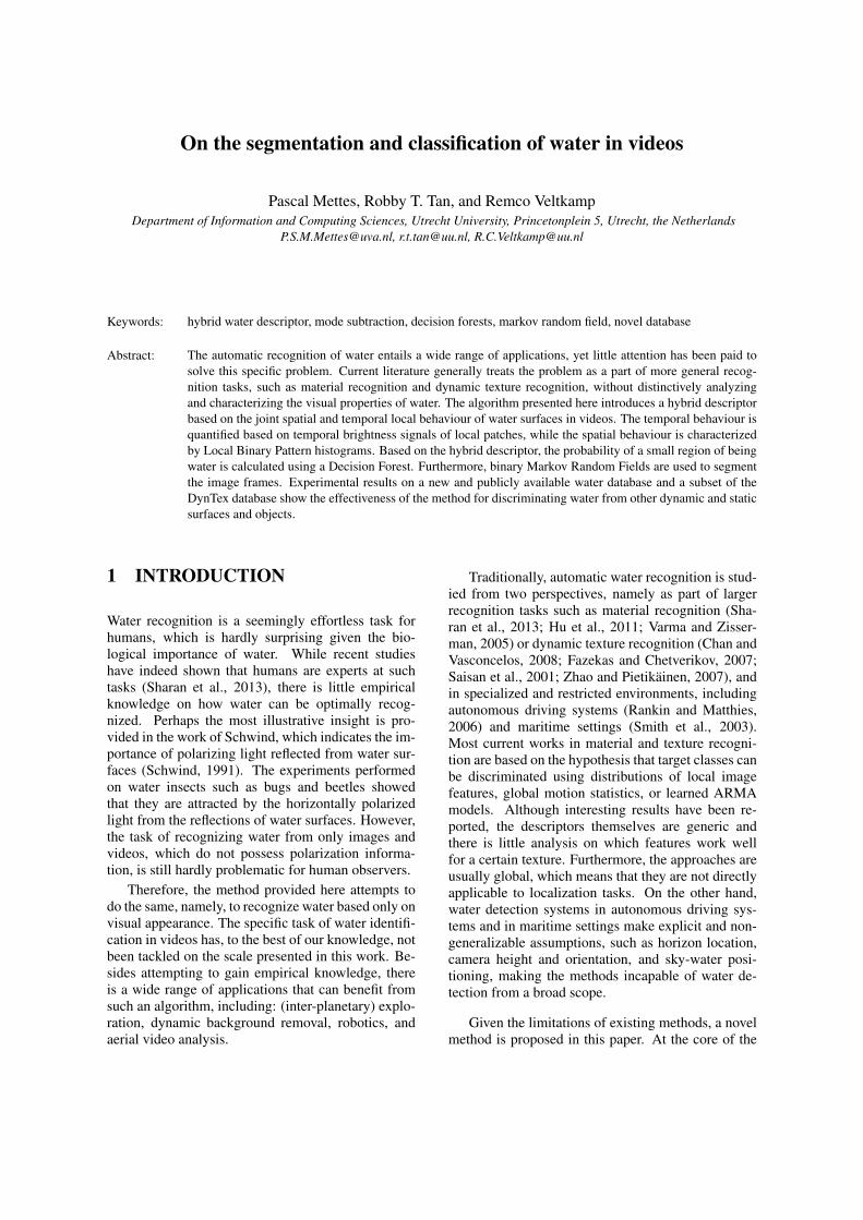
(a) Canal. (b) Fountain. (c) Lake. (d) Ocean. (e) Stream. (f) Pond.

(g) River. (h) Non-water.Figure 1: Exemplary frames of categories in the water database.

method is a hybrid descriptor based on local spatialand temporal information. First, the input video ispre-processed to remove the background reflectionsand water colour, leaving only the residual image se-quence, which conveys the motion of water. Given theresidual images, local descriptors are extracted andclassified using a Decision Forest (Bochkanov, 2013;Criminisi et al., 2012). The trained Forest can then beutilized to perform local classification for a collectionof test sequences, where the probabilities are providedto a binary Markov Random Field to generate a seg-mentation for the frames in the test sequences basedon the presence or absence of water.

Since this work is specifically aimed at water de-tection and given the supervised nature of the algo-rithm, a second contribution of this work is the intro-duction of a new database. The water database, fur-ther elaborated at the end of this section, consists ofa set of complex natural scenes with a wide varietyof water surfaces. Experimental evaluation on thisdatabase and on the DynTex database (Peteri et al.,2010) shows the effectiveness of the proposed methodfor both video classification and spatio-temporal seg-mentation.

The paper is organized as follows. This Section isconcluded with an elaboration of the water database,while Section 2 discusses the works related to com-putational water recognition. Section 3 provides ananalysis of the temporal and spatial behaviour of wa-ter, the descriptors derived from that analysis, and theprocess of local classification. This is followed bythe global segmentation step in Section 4. Section 5shows the experimental evaluation on the databasesand the paper is concluded in Section 6.

1.1 Water Database

As stated above, experimental evaluation is per-formed in this work on a novel database, in order to

tackle the challenge problem of water detection1. Al-though databases used in dynamic texture recognitiondo contain water videos (Peteri et al., 2010), they donot contain water videos in the quantity and varietydesired for water recognition and localization. Thenovel water database contains a set of positive andnegative videos (i.e. water and non-water videos),from a wide variety of natural scenes. In total, thedatabase consists of 260 videos, where each videocontains between 750 and 1500 frames, all with aframe size of 800×600. The positive class consists of160 videos of predominantly 7 scenes; oceans, foun-tains, ponds, rivers, streams, canals, and lakes. Thenegative class on the other hand can be representedby any other scene. In the database, categories withseemingly similar spatial and temporal characteristicsare chosen, including trees, fire, flags, clouds/steam,and vegetation. Examples of the categories of thedatabase are shown in Fig. 1. Since the focus of thiswork is aimed at characterizing the behaviour of wa-ter, camera motion is considered a separate problemand it is therefore not integrated into the database.

2 RELATED WORK

Original work on material classification attemptedto discriminate materials photographed in laboratorysettings, e.g. based on distributions of Gabor filter re-sponses (Varma and Zisserman, 2005) or image patchexemplars (Varma and Zisserman, 2009). More re-cently, the classification problem has shifted to thereal-world domain with the Flickr Materials Database(Sharan et al., 2009), which includes water as one ofthe target classes. Current approaches attempt to dis-criminate materials based on concatenations of localimage feature distributions (Hu et al., 2011; Sharanet al., 2013). Although it is possible to apply these ap-proaches to the more specific problem of water recog-

1For detail and downloads, visit the author’s webpage.

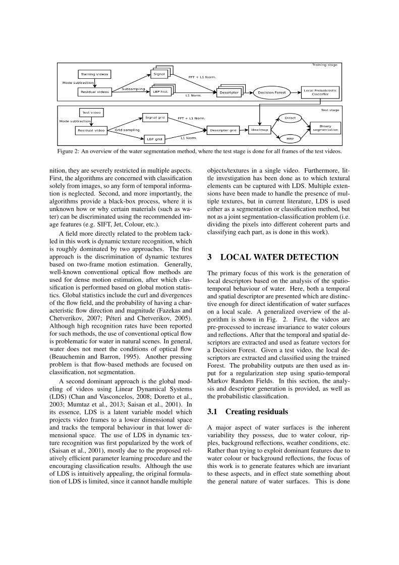
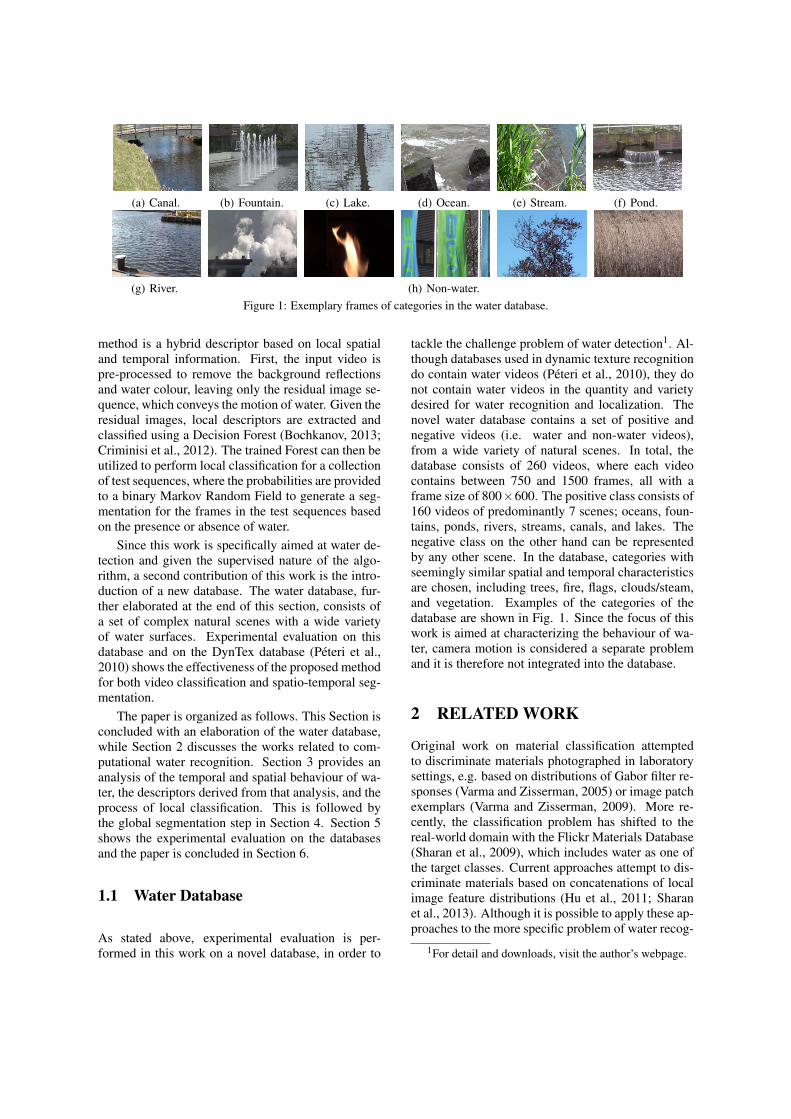
Figure 2: An overview of the water segmentation method, where the test stage is done for all frames of the test videos.

nition, they are severely restricted in multiple aspects.First, the algorithms are concerned with classificationsolely from images, so any form of temporal informa-tion is neglected. Second, and more importantly, thealgorithms provide a black-box process, where it isunknown how or why certain materials (such as wa-ter) can be discriminated using the recommended im-age features (e.g. SIFT, Jet, Colour, etc.).

A field more directly related to the problem tack-led in this work is dynamic texture recognition, whichis roughly dominated by two approaches. The firstapproach is the discrimination of dynamic texturesbased on two-frame motion estimation. Generally,well-known conventional optical flow methods areused for dense motion estimation, after which clas-sification is performed based on global motion statis-tics. Global statistics include the curl and divergencesof the flow field, and the probability of having a char-acteristic flow direction and magnitude (Fazekas andChetverikov, 2007; Peteri and Chetverikov, 2005).Although high recognition rates have been reportedfor such methods, the use of conventional optical flowis problematic for water in natural scenes. In general,water does not meet the conditions of optical flow(Beauchemin and Barron, 1995). Another pressingproblem is that flow-based methods are focused onclassification, not segmentation.

A second dominant approach is the global mod-eling of videos using Linear Dynamical Systems(LDS) (Chan and Vasconcelos, 2008; Doretto et al.,2003; Mumtaz et al., 2013; Saisan et al., 2001). Inits essence, LDS is a latent variable model whichprojects video frames to a lower dimensional spaceand tracks the temporal behaviour in that lower di-mensional space. The use of LDS in dynamic tex-ture recognition was first popularized by the work of(Saisan et al., 2001), mostly due to the proposed rel-atively efficient parameter learning procedure and theencouraging classification results. Although the useof LDS is intuitively appealing, the original formula-tion of LDS is limited, since it cannot handle multiple

objects/textures in a single video. Furthermore, lit-tle investigation has been done as to which texturalelements can be captured with LDS. Multiple exten-sions have been made to handle the presence of mul-tiple textures, but in current literature, LDS is usedeither as a segmentation or classification method, butnot as a joint segmentation-classification problem (i.e.dividing the pixels into different coherent parts andclassifying each part, as is done in this work).

3 LOCAL WATER DETECTION

The primary focus of this work is the generation oflocal descriptors based on the analysis of the spatio-temporal behaviour of water. Here, both a temporaland spatial descriptor are presented which are distinc-tive enough for direct identification of water surfaceson a local scale. A generalized overview of the al-gorithm is shown in Fig. 2. First, the videos arepre-processed to increase invariance to water coloursand reflections. After that the temporal and spatial de-scriptors are extracted and used as feature vectors fora Decision Forest. Given a test video, the local de-scriptors are extracted and classified using the trainedForest. The probability outputs are then used as in-put for a regularization step using spatio-temporalMarkov Random Fields. In this section, the analy-sis and descriptor generation is provided, as well asthe probabilistic classification.

3.1 Creating residuals

A major aspect of water surfaces is the inherentvariability they possess, due to water colour, rip-ples, background reflections, weather conditions, etc.Rather than trying to exploit dominant features due towater colour or background reflections, the focus ofthis work is to generate features which are invariantto these aspects, and in effect state something aboutthe general nature of water surfaces. This is done

(a)

(b)Figure 3: A typical frame, temporal mode, and residual for 2 videos.

by first obtaining the water colour as well as back-ground reflections, and then removing them, leavingonly residual images.

The aim of the residual frames is to highlight wa-ter ripples, instead of reflections. This is realized byperforming temporal mode subtraction for each pixel:

Rt(x,y)[c] = |It(x,y)[c]−M(x,y)[c]|, (1)

for each c ∈ {R,G,B} separately, where M(x,y) de-notes the temporal mode of pixel (x,y). The temporalmode of a single pixel for a single colour channel canbe computed as follows:

M(x,y)[c] = maxp

T

∑t=1

1{It(x,y)[c] = p}, (2)

where T denotes the total number of frames and 1{·}is the indicator function. A typical frame, temporalmode, and corresponding residual frame of 2 videosare shown in Fig. 3. Note that this simple proceduredoes not remove all reflections, but it can successfullyfind the most dominant elements of reflection, suchthat the residual frames highlight water ripples.

3.2 Local temporal descriptor

The idea behind the temporal water descriptor is thatthe water ripples indicate the motion characteristics.The motion characteristics of water are hypothesizedto constitute several aspects. Most notably, it is hy-pothesized here that this type of motion is gradual andrepetitive, since ripples re-occur at the same locationover time. Other dynamic and static processes mightpartially share the local temporal properties of water,but not statistically to the same extent.

Based on the defined hypotheses, the next stepis to create a descriptor which judges a local spatio-temporal patch on these hypotheses. To achieve this,

(a)

(b)

(c)

(d)Figure 4: Four exemplary frames and sample signals.

an m-dimensional signal is first introduced, whichrepresents the mean brightness value of an n×n patchfor m consecutive frames at exactly the same location.The result is a list of brightness values which can beseen as a 1-dimensional signal. Fig. 4 shows mul-

(a) Original signals. (b) FT of signals (c) Norm. FT of signals

(d) LBP (e) HybridFigure 5: Isomap projections of sample locations of trees (blue) and water (red). The Figure shows how using normalizedFourier Transforms improves separation using temporal information (a,b,c). More interesting, it clearly shows that fusingtemporal and spatial information creates a further boost in separation (c,d,e).

tiple examples of water and non-water scenes, alongwith a mean brightness signal of a selected location.From the Figure, the initial thoughts regarding regu-larity and repetition are already clearly visible.

Given the m-dimensional signals, an immediatethought is to use them directly as the descriptor. Thedirect use of the signal itself as the descriptor is how-ever erroneous, due to lack of invariance. Signalswith similar levels of smoothness and regularity canhave a large distance when comparing the signals di-rectly. A descriptor based on the m-dimensional sig-nal should in effect be invariant to temporal shifts,brightness shifts, and brightness amplitudes. Ratherthan creating a distance measure which explicitly en-forces these types of invariance by means of nor-malization and distance recalculation for all possibletemporal and brightness shifts, a descriptor is cre-ated here by extracting the signal characteristics us-ing the 1-dimensional Fourier Transform. For anm-dimensional signal S, the corresponding FourierTransform F is also m-dimensional, where each com-ponent i ∈ {1,m} is computed as:

Fi = |m

∑j=1

S je−2πi j√−1/m|. (3)

In other words, from the signal, an m-dimensional de-scriptor [F1, ..,Fm] is computed. Although this de-scriptor is invariant to the temporal and brightnessshifts, it is not invariant to brightness amplitudes.Therefore, the final temporal descriptor is generated

by performing L1-normalization on the components,such that two signals are compared by the distributionof the Fourier Transform, i.e.:

Fi =|∑m

j=1 S je−2πi j√−1/m|

∑mk=1 |∑m

l=1 Sle−2πkl√−1/m|

. (4)

A practical justification of using the L1-normalized Fourier Transform as the temporaldescriptor is shown in Fig. 5. The Figure displaysthe Isomap projection (Tenenbaum et al., 2000)of samples taken from water and tree videos. Anideal local descriptor has linear separability in theoriginal feature space. For visualization purposes,the projected feature space is used here, but the fullfeature space is used in the classification. As can beseen in Fig. 5(a) and Fig. 5(b), the original signalsand their Fourier Transform are rather impractical interms of classification, while a separation is clearlyvisible in Fig. 5(c), although there is an area ofoverlap.

The choice of signal length m is a trade-off. Ide-ally for recognition, m is equal to the total numberof frames in the video, since the longer the signal, theless likely it is that non-water surfaces mimic the tem-poral behaviour of water. On the other hand, this ap-proach makes it impossible to detect temporal discon-tinuities. Since the focus lies primarily on discrimina-tions while still being able to detect obvious outliers,m is set to 200 frames here.

3.3 Local spatial descriptor

The above defined descriptor captures the temporalbehaviour of water, but ignores the local spatial in-formation, most notably the spatial layout of waterwaves and ripples. Given that water waves, ripples,and fountains are highly deformable, a descriptor isdesired which provides spatial information on a lo-cal patch without requiring an explicit model of waterwaves. To meet this desire, the local spatial character-istics of water surfaces are extracted using Local Bi-nary Pattern histograms (Zhao and Pietikainen, 2007).For a single pixel, the Local Binary Pattern is com-puted by comparing the grayscale values of the pixelto a set of local spatial neighbours. In this work, the 8direct neighbours of a pixel are used for comparison.As such, the Local Binary Pattern value of a singlepixel is computed as:

LBP8,1(gc) =7

∑p=0

H(gcp−gc)2p, (5)

where gc denotes the center pixel for which the LBPvalue is computed, {gc

i }7i=0 denotes the set of direct

neighbours of gc, and H(·) is the well-known discreteHeaviside step function, defined as:

H(x) ={

1 x≥ 00 x < 0. (6)

Since 8 neighbours are used in the comparison, thecorresponding LBP value can take 28 = 256 values.In order to compute a LBP histogram of a local patch,the LBP values of the pixels in the patch are computedand placed in their corresponding integer bins of the256-dimensional histogram. The resulting histogramis normalized afterwards.

As stated above, a primary justification for the useof Local Binary Pattern histograms as a spatial de-scriptor is due to the pseudo-orderless nature of thedescriptor, which means that water waves do not needto be modeled explicitly. Furthermore, the high di-mensionality of the histograms provide desirable dis-crimination abilities. Similar to the temporal descrip-tor, the practical validity of the LBP histograms canbe shown by examining the projected feature space.The early fusion (Snoek et al., 2005) of the temporaland spatial descriptors into a hybrid descriptor, resultsin a feature space where its projection is almost nearlylinearly separable for the randomly selected localpatch, as can be seen in Fig. 5(e). The importance of apseudo-orderless spatial descriptor came to light afterthe investigations into explicit water modeling turnedout to be impractical. This conclusion is consistentwith literature on dynamic texture recognition. Forexample in overlapping work of Zhao and Pietkainen,

multiple extensions of LBP have been proposed, suchas VLBP (Zhao and Pietikainen, 2006) and LBP-TOP(Zhao and Pietikainen, 2007). VLBP is however im-practical for local direct identification, since each his-togram would have a length of 214 or even 226, dueto the fact that both spatial and temporal neighboursneed to be compared against the central pixel. Similarstatements can be made regarding LBP-TOP. There-fore, the original purely spatial LBP descriptor is usedhere.

3.4 Probabilistic classification

Now that the behaviour of water on a local temporaland spatial level have been defined, the next step isto exploit the descriptors for probabilistic classifica-tion. Contrary to computing distributions of descrip-tors as is usual in global classification tasks, the de-scriptors are used directly as feature vectors for prob-abilistic classification using Decision Forests. In thetraining stage of the algorithm, the descriptors are ex-tracted from the training videos and used as featurevectors for the Decision Forest. Since the numberof patches per frame can be considerably large, se-lecting patches from a uniform grid for each frame ofeach training video is undesirable, given the amountof time required for training. For that reason, a ran-dom sampling approach is employed by selecting asmall number of patches per frame per training video.

Given the use of random sampling, roughly 2500local patches are selected per training video. The456-dimensional feature vectors for the patches of alltraining videos are then fed to the Decision Forest forprobabilistic classification. The primary parametersof the forest - the number of trees and the randomnessfactor - can be set using cross-validation.

In the testing stage, descriptors need to be ex-tracted from all parts of the frames of the test videos.Therefore patches are extracted from a dense rectan-gular grid. The descriptors yielded from the grid areindividually given to the trained forest, yielding a ma-trix of probability outputs, which can be seen as aheatmap. A major advantage of direct local classi-fication is that each local part of the video is classi-fied separately. However, since this approach yields agreat number of separate classifications, it can be ex-pected that multiple miss-classifications occur withinand between the frames of a test video. For that rea-son, a last step of this algorithm is the use of MarkovRandom Fields for spatio-temporal regularization.

4 HEATMAP REGULARIZATION

The additional information on the probabilistic(un)certainty of classified local patches, instead of di-rect decisions, opens up the possibility to discrete op-timization on the heatmaps. The discrete optimizationtakes the form in this work of a Markov Random Field(Boykov and Kolmogorov, 2004), which serves as aregularization step. More formally, the optimizationproblem of the MRF can be stated as a minimizationproblem with the following objective function:

f (x) = ∑p∈V

Vp(xp)+λ ∑(p,q)∈C

Vpq(xp,xq), (7)

with V the elements of the heatmap, and C the set ofall cliques. The first term of the objective function -the data term - is then defined as:

Vp(xp) =

{1−Mp if xp is waterMp otherwise (8)

where Mp denotes the probability of node (i.e.heatmap pixel) p of begin water. The second term- the prior term - is defined such that different labelswithin cliques are penalized:

Vpq(xp,xq) = |xp− xq|, (9)

given that the label water is defined as 1 and the labelnon-water is defined as 0.

An interesting element within the MRF formu-lation are the cliques. Rather than only enforc-ing similarity between neighbouring pixels in a sin-gle heatmap, a form of temporal regularization isalso desired, since water location is not expectedto change sharply over time. Therefore, a spatio-temporal Markov Random Field formulation is optedhere, where each element of the heatmap is connectedto both its 4 spatial neighbours and 2 temporal neigh-bours.

An important element in the minimization proce-dure is the relative weight of the probabilities (dataterm) and spatial consistency (prior term), denoted byλ in Eq. 7. For a low value for λ, the individual prob-abilities are deemed important, resulting in a segmen-tation with a lot of detail, but also with outliers. Onthe other hand, a high value for λ results in a seg-mentation with little outliers, at the cost of loss of de-tail at borders between water and non-water regions.The influence of the λ term is evaluated in Section 5.Since not all pixels on a single frame are classified,the binarized heatmap only contains the segmentationresult for a subset of the pixels on a rectangular grid.The segmentation results are therefore bi-cubicly in-terpolated such that each pixel is classified as eitherbeing water or non-water.

5 EXPERIMENTAL EVALUATION

The effectiveness of the algorithm presented in theprevious sections is validated on the novel waterdatabase by examining both the segmentation qual-ity (i.e. the classification of each pixel of each frame)and the classification quality (i.e. the classification ofa whole video with a binary mask). In the implemen-tation of the algorithm, the videos of the database arerandomly split with a 60/40 ratio into a train and testset. For each test video, the segmentation is computedfor 250 frames.

In the evaluation, the segmentation fit of the videois defined as the average of the fit of the individualsegmentations with the supplemented binary mask.Formally, the segmentation fit S of a segmented videoV compared to a mask M is computed as:

S(V,M) =∑|V |i=1 s(Vi,m)

|V |×100%, (10)

where |V | denotes the number of frames in V , Vi de-notes the ith frame, and s(Vi,M) is defined as:

s(Vi,M) = 1−∑

Wx=1 ∑

Hy=1 |Vi[x,y]−m[x,y]|

W ×H, (11)

with W and H for resp. the width and height of thevideo and the pixel values of the segmentations andthe mask are 1 for water and 0 for non-water. Givena set of segmentations and a binary mask, the wholevideo can be classified as water if the ratio of waterpixels in the mask region is at least a half, and non-water otherwise.

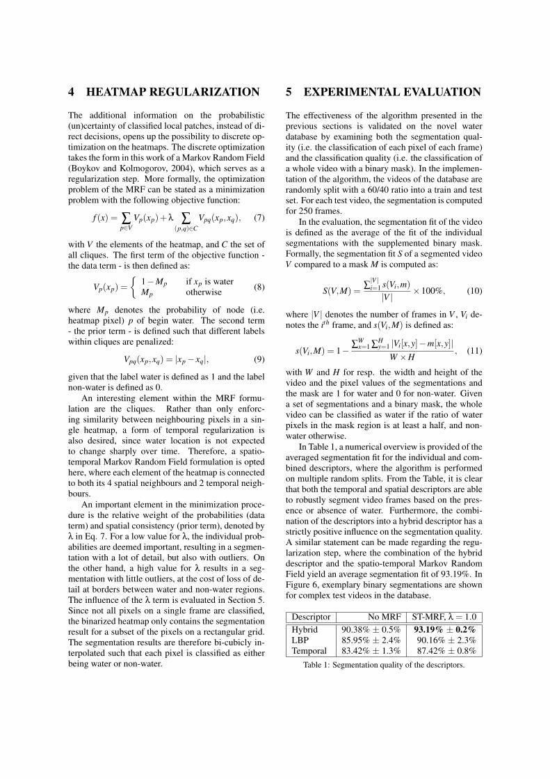
In Table 1, a numerical overview is provided of theaveraged segmentation fit for the individual and com-bined descriptors, where the algorithm is performedon multiple random splits. From the Table, it is clearthat both the temporal and spatial descriptors are ableto robustly segment video frames based on the pres-ence or absence of water. Furthermore, the combi-nation of the descriptors into a hybrid descriptor has astrictly positive influence on the segmentation quality.A similar statement can be made regarding the regu-larization step, where the combination of the hybriddescriptor and the spatio-temporal Markov RandomField yield an average segmentation fit of 93.19%. InFigure 6, exemplary binary segmentations are shownfor complex test videos in the database.

Descriptor No MRF ST-MRF, λ = 1.0Hybrid 90.38% ± 0.5% 93.19% ± 0.2%LBP 85.95% ± 2.4% 90.16% ± 2.3%Temporal 83.42% ± 1.3% 87.42% ± 0.8%

Table 1: Segmentation quality of the descriptors.

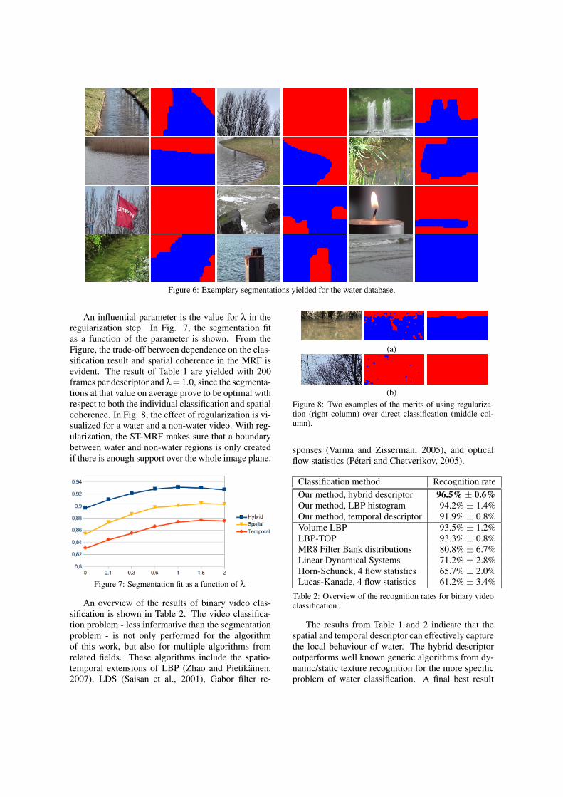
Figure 6: Exemplary segmentations yielded for the water database.

An influential parameter is the value for λ in theregularization step. In Fig. 7, the segmentation fitas a function of the parameter is shown. From theFigure, the trade-off between dependence on the clas-sification result and spatial coherence in the MRF isevident. The result of Table 1 are yielded with 200frames per descriptor and λ= 1.0, since the segmenta-tions at that value on average prove to be optimal withrespect to both the individual classification and spatialcoherence. In Fig. 8, the effect of regularization is vi-sualized for a water and a non-water video. With reg-ularization, the ST-MRF makes sure that a boundarybetween water and non-water regions is only createdif there is enough support over the whole image plane.

Figure 7: Segmentation fit as a function of λ.

An overview of the results of binary video clas-sification is shown in Table 2. The video classifica-tion problem - less informative than the segmentationproblem - is not only performed for the algorithmof this work, but also for multiple algorithms fromrelated fields. These algorithms include the spatio-temporal extensions of LBP (Zhao and Pietikainen,2007), LDS (Saisan et al., 2001), Gabor filter re-

(a)

(b)Figure 8: Two examples of the merits of using regulariza-tion (right column) over direct classification (middle col-umn).

sponses (Varma and Zisserman, 2005), and opticalflow statistics (Peteri and Chetverikov, 2005).

Classification method Recognition rateOur method, hybrid descriptor 96.5% ± 0.6%Our method, LBP histogram 94.2% ± 1.4%Our method, temporal descriptor 91.9% ± 0.8%Volume LBP 93.5% ± 1.2%LBP-TOP 93.3% ± 0.8%MR8 Filter Bank distributions 80.8% ± 6.7%Linear Dynamical Systems 71.2% ± 2.8%Horn-Schunck, 4 flow statistics 65.7% ± 2.0%Lucas-Kanade, 4 flow statistics 61.2% ± 3.4%

Table 2: Overview of the recognition rates for binary videoclassification.

The results from Table 1 and 2 indicate that thespatial and temporal descriptor can effectively capturethe local behaviour of water. The hybrid descriptoroutperforms well known generic algorithms from dy-namic/static texture recognition for the more specificproblem of water classification. A final best result

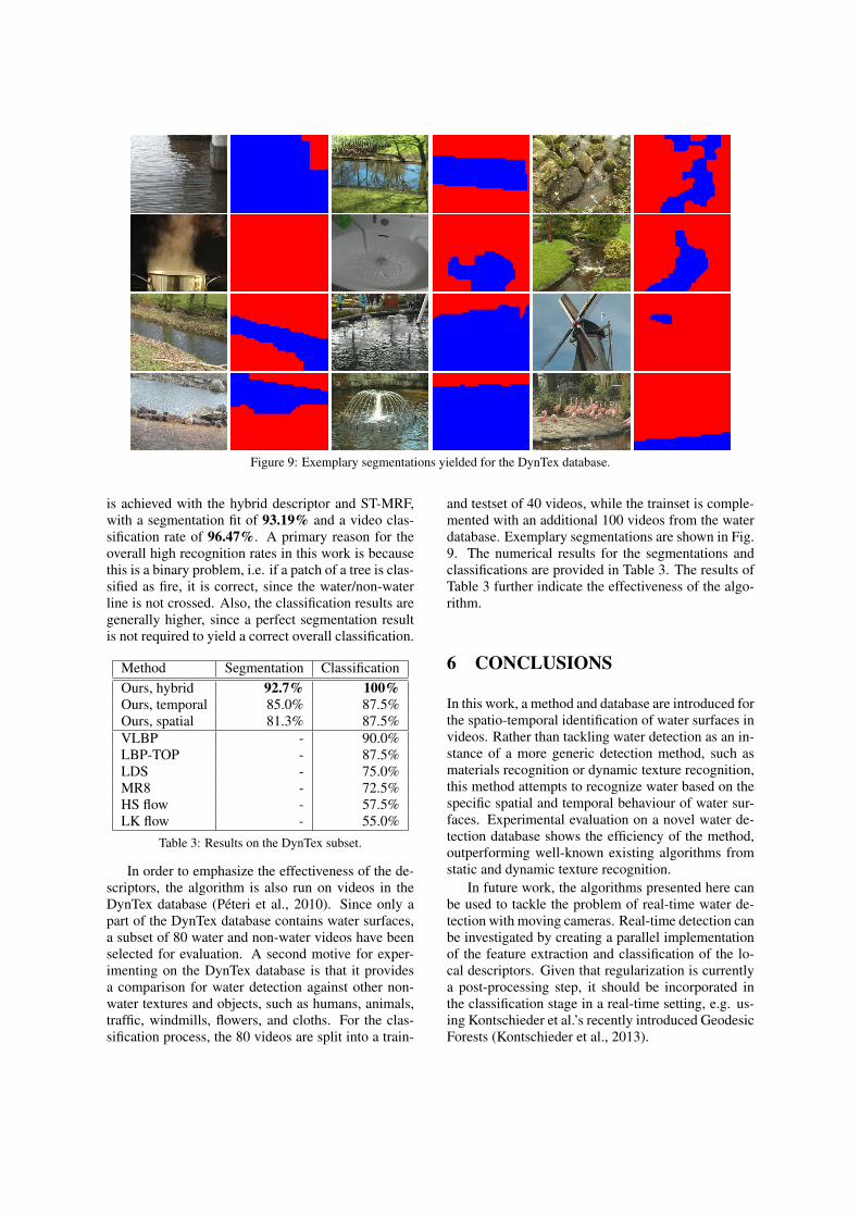
Figure 9: Exemplary segmentations yielded for the DynTex database.

is achieved with the hybrid descriptor and ST-MRF,with a segmentation fit of 93.19% and a video clas-sification rate of 96.47%. A primary reason for theoverall high recognition rates in this work is becausethis is a binary problem, i.e. if a patch of a tree is clas-sified as fire, it is correct, since the water/non-waterline is not crossed. Also, the classification results aregenerally higher, since a perfect segmentation resultis not required to yield a correct overall classification.

Method Segmentation ClassificationOurs, hybrid 92.7% 100%Ours, temporal 85.0% 87.5%Ours, spatial 81.3% 87.5%VLBP - 90.0%LBP-TOP - 87.5%LDS - 75.0%MR8 - 72.5%HS flow - 57.5%LK flow - 55.0%

Table 3: Results on the DynTex subset.

In order to emphasize the effectiveness of the de-scriptors, the algorithm is also run on videos in theDynTex database (Peteri et al., 2010). Since only apart of the DynTex database contains water surfaces,a subset of 80 water and non-water videos have beenselected for evaluation. A second motive for exper-imenting on the DynTex database is that it providesa comparison for water detection against other non-water textures and objects, such as humans, animals,traffic, windmills, flowers, and cloths. For the clas-sification process, the 80 videos are split into a train-

and testset of 40 videos, while the trainset is comple-mented with an additional 100 videos from the waterdatabase. Exemplary segmentations are shown in Fig.9. The numerical results for the segmentations andclassifications are provided in Table 3. The results ofTable 3 further indicate the effectiveness of the algo-rithm.

6 CONCLUSIONS

In this work, a method and database are introduced forthe spatio-temporal identification of water surfaces invideos. Rather than tackling water detection as an in-stance of a more generic detection method, such asmaterials recognition or dynamic texture recognition,this method attempts to recognize water based on thespecific spatial and temporal behaviour of water sur-faces. Experimental evaluation on a novel water de-tection database shows the efficiency of the method,outperforming well-known existing algorithms fromstatic and dynamic texture recognition.

In future work, the algorithms presented here canbe used to tackle the problem of real-time water de-tection with moving cameras. Real-time detection canbe investigated by creating a parallel implementationof the feature extraction and classification of the lo-cal descriptors. Given that regularization is currentlya post-processing step, it should be incorporated inthe classification stage in a real-time setting, e.g. us-ing Kontschieder et al.’s recently introduced GeodesicForests (Kontschieder et al., 2013).

ACKNOWLEDGEMENTS

This research is supported by the FES project COM-MIT. Furthermore, we would like to thank RenaudPeteri for providing access to the DynTex database.

REFERENCES

Beauchemin, S. and Barron, J. (1995). The computationof optical flow. ACM Computing Surveys, 27(3):433–466.

Bochkanov, S. (1999-2013). Alglib software library(www.alglib.net).

Boykov, Y. and Kolmogorov, V. (2004). An experimentalcomparison of min-cut/max-flow algorithms for en-ergy minimization in vision. PAMI.

Chan, A. and Vasconcelos, N. (2008). Modeling, cluster-ing, and segmenting video with mixtures of dynamictextures. PAMI, 30(5):909–926.

Criminisi, A., Shotton, J., and Konukoglu, E. (2012). De-cision forests. Foundations and Trends in ComputerGraphics and Vision, 7(2):81–227.

Doretto, G., Cremers, D., Favaro, P., and Soatto, S. (2003).Dynamic texture segmentation. ICCV, 2:1236–1242.

Fazekas, S. and Chetverikov, D. (2007). Analysis and per-formance evaluation of optical flow features for dy-namic texture recognition. SPIC, 22:680–691.

Hu, D., Bo, L., and Ren, X. (2011). Toward robust materialrecognition for everyday objects. BMVC, pages 48.1–48.11.

Kontschieder, P., Kohli, P., Shotton, J., and Criminisi, A.(2013). Geof: Geodesic forests for learning coupledpredictors. CVPR.

Mumtaz, A., Coviello, E., Lanckriet, G., and Chan, A.(2013). Clustering dynamic textures with the hier-archical em algorithm for modeling video. PAMI,35(7):1606–1621.

Peteri, R. and Chetverikov, D. (2005). Dynamic texturerecognition using normal flow and texture regularity.PRIA, 3523:223–230.

Peteri, R., Fazekas, S., and Huiskes, M. (2010). Dyntex: Acomprehensive database of dynamic textures. PatternRecognition Letters, 31(12):1627–1632.

Rankin, A. and Matthies, L. (2006). Daytime water de-tection and localization for unmanned ground vehicleautonomous navigation. Proceeding of the 25th ArmyScience Conference.

Saisan, P., Doretto, G., Wu, Y. N., and Soatto, S. (2001).Dynamic texture recognition. CVPR, 2:II–58–II–63.

Schwind, R. (1991). Polarization vision in water insects andinsects living on a moist substrate. Journal of Com-parative Physiology A, 169(5):531–540.

Sharan, L., Liu, C., Rosenholtz, R., and Adelson, E.(2013). Recognizing materials using perceptually in-spired features. IJCV, pages 1–24.

Sharan, L., Rosenholtz, R., and Adelson, E. (2009). Mate-rial perception: What can you see in a brief glance?[abstract]. Journal of Vision, 9(8):784.

Smith, A., Teal, M., and Voles, P. (2003). The statisti-cal characterization of the sea for the segmentation ofmaritime images. Video/Image Processing and Multi-media Communications, 2:489–494.

Snoek, C., Worring, M., and Smeulders, A. (2005). Earlyversus late fusion in semantic video analysis. In Pro-ceedings of the 13th annual ACM international con-ference on Multimedia, pages 399–402. ACM.

Tenenbaum, J., de Silva, V., and Langford, J. (2000). Aglobal geometric framework for nonlinear dimension-ality reduction. Science, 290(5500):2319–2323.

Varma, M. and Zisserman, A. (2005). A statistical approachto texture classification from single images. IJCV,62(1):61–81.

Varma, M. and Zisserman, A. (2009). A statistical ap-proach to material classification using image patch ex-emplars. PAMI, 31(11):2032–2047.

Zhao, G. and Pietikainen, M. (2006). Local binary patterndescriptors for dynamic texture recognition. ICPR,2:211–214.

Zhao, G. and Pietikainen, M. (2007). Dynamic texturerecognition using local binary patterns with an appli-cation to facial expressions. PAMI, 29(6):915–928.