On the Spatial Dynamics of the Solutionto the Stochastic Heat Equation

Sigurd Assing (joint with J. Bichard)Deptartment of Statistics

University of Warwick

s.assing@warwick.ac.uk

Probability Seminar

Berkeley, October 23, 2013

Wikipedia-stub

Stochastic partial differential equations (SPDEs) are similar toordinary stochastic differential equations. They are essentially partialdifferential equations that have random forcing terms and coefficients.They can be exceedingly difficult to solve. However, they have strongconnections with quantum field theory and statistical mechanics.

One difficulty encountered when dealing with stochastic PDEs is their lack ofregularity. For example, one of the most classical SPDEs is given by thestochastic heat equation which can formally be written as

∂tu = ∆u + η

where η denotes space-time white noise and ∆ is the Laplacian. In one spacedimension, solutions to this equation are only almost 1/2-Holder continuous inspace and 1/4-Holder continuous in time. For dimensions two and higher,solutions are not even function-valued, but can be made sense of as randomdistributions.

2

Easy Examples

Whittle (1954,1963) Gaussian field:

(κ−∆)α/2u = η where α = ν + d/2

which is recently (Lindgren et al.) used to model annual meantemperatures, for example.

Another example can already be found in:

Walsh, J.B.: An introduction to stochastic partial differential equations. Ecoled’ete de probabilites de Saint-Flour (1984). Lecture Notes in Math. 1180.Berlin: Springer, 1986

3

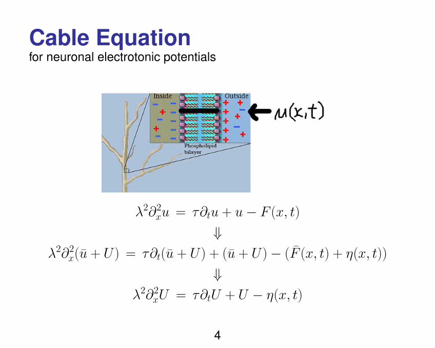
Cable Equationfor neuronal electrotonic potentials

λ2∂2xu = τ∂tu + u− F (x, t)

⇓λ2∂2x(u + U) = τ∂t(u + U) + (u + U)− (F (x, t) + η(x, t))

⇓λ2∂2xU = τ∂tU + U − η(x, t)

4

What is an interesting question?

Find law of

ξ = infx ≥ x0 : maxt≥0

[u(x, t) + U(x, t)] ≤ c

which is

first location above the point of injection of initial current

such that

the electrotonic potential is always below a level c.

5

6

Intermezzo

For a Wiener trajectory

defineτc = inft ≥ 0 : Wt ≥ c.

HOW do you get the law of τc?

7

Two answers:

1) Find the joint law of Wt and maxs≤tWs. This requires reflectionprinciple and strong Markov property of the Wiener process.

2) Go straight for the Laplace transform Ee−ντc, ν > 0. Thisrequires Itos’ formula hence a martingale problem associated withthe Wiener process.

8

Back to the neurons:

Want law of

ξ = infx ≥ x0 : maxt≥0

[u(x, t) + U(x, t)] ≤ c

where

= u(x, t) + U(x, t)

andλ2∂2xU = τ∂tU + U − η(x, t).

9

Note:

• Markov property of U implies Markov property of u because u isdeterministic.

• The Markov property of U we need is in x-direction.

• There is a ‘sharp’ Markov property of U in t-direction. This isbecause the cable equation can be rewritten as an SDE

dU(·, t) = AU(·, t) dt +1

τdWt(·) where A =

λ2

τ∂2x −

Id

τ

in a function space and that’s how it is solved usually.

• Otherwise, U satisfies a so-called germ Markov property.

10

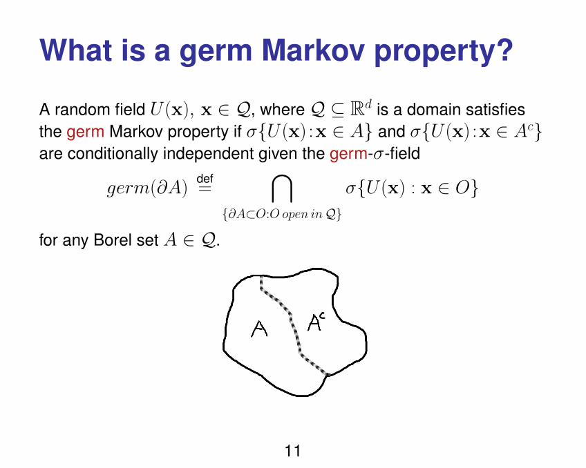
What is a germ Markov property?

A random field U(x), x ∈ Q, whereQ ⊆ Rd is a domain satisfiesthe germ Markov property if σU(x) :x ∈ A and σU(x) :x ∈ Acare conditionally independent given the germ-σ-field

germ(∂A)def=

⋂∂A⊂O:O open inQ

σU(x) : x ∈ O

for any Borel set A ∈ Q.

11

Difference between:

t-direction

x-direction

for Cable equation whenQ = (x0,∞)× (0,∞).

12

Recall the two methods

1) Find the joint law of Wt and maxs≤tWs. This requires reflectionprinciple and strong Markov property of the Wiener process.

2) Go straight for the Laplace transform Ee−ντc, ν > 0. Thisrequires Itos’ formula hence a martingale problem associated withthe Wiener process.

for finding law of hitting time in thecase of a 1-dim Wiener process.

13

This would not work for

ξ = infx ≥ x0 : maxt≥0

[u(x, t) + U(x, t)] ≤ c

if one only has a germ Markov property in x-direction as one does notget a martingale problem associated with a germ Markov process.

One wants to knowif there is a σ-algebra included in germ ( x × (0,∞) ) so thatx 7→ U(x, ·) is still Markovian relative to this smaller σ-algebra butalso satisfies an associated martingale problem.

And, because we are dealing with SPDEs, it is very likely that aσ-algebra generated by certain partial derivatives of U(x, t) withrespect to x would serve the purpose.

14

Our main result, EJP 18 (2013), states

that the above can be achieved in the case of the stochastic heatequation

∂2xu = ∂tu− η(x, t) in Q = R× (0,∞)

with space-time white noise external forcing.

We find a martingale problem for the pair of processes(u(x, ·), ∂xu(x, ·)), x ≥ x0, which is given by an unbounded operatorwe explicitly calculate using the technique of enlargement of filtration.

By showing the uniqueness of the martingale problem, we then getthe strong Markov property of (u(x, ·), ∂xu(x, ·)), x ≥ x0.

15

However

all our calculations are based on only two ingredients:

• a Green’s function for

Lu = −η in Q

where L is a linear partial differential operator of elliptic orparabolic type and η stands for a multi-parameter noise.

• the covariance of a Gaussian noise η.

16

Therefore

following our scheme of calculations but using a different Green’sfunction or covariance would produce similar results with respect toother linear SPDEs.

In this talk I will also give some details for the cable equation

∂2xu = ∂tu + u− η(x, t) in Q = R× (0,∞)

because I used it for motivation ,.

Unfortunately the outcome is not as explicit as in the case of thestochastic heat equation.

17

Further Comments:

• The explicit calculations can be involved and, in the case of thestochastic heat equation, we think that they are interesting inthemselves. That’s why we restrict ourselves to this importantexample performing a rather detailed analysis.

• We think that drift perturbed elliptic or parabolic equations

Lu = −η + f (u) in Q

can be transformed into linear equations by applying Kusuoka orGirsanov transforms. This has been done to show the germMarkov property of solutions to these equations.

18

Notation

The heat kernel

g(y, s ;x, t)def=

1√4π(t− s)

exp−(x− y)2

4(t− s)1(s,∞)(t)

is considered a function

g : [ R×R ]× [ R×R ]→ R.

We use f1 ∗ f2 to denote the convolution of functions f1, f2 : R→ Rand write fi for their Laplace transform

fi(ν)def=

∫ ∞0

fi(t)e−νt dt, ν > 0, i = 1, 2.

Note that(f111(0,∞)) ∗ (f211(0,∞)) = f1 f2.

19

The following domains

Q+ = R× (0,∞) and Qy+ = (y,∞)× (0,∞), y ∈ R,

will be frequently used.

The symbol D is reserved for C∞c ((0,∞)), the space of smoothfunctions on (0,∞) with compact support.

〈· ; ·〉 denotes the scalar product in L2([0,∞)) and, whenever thedual pairing between a topological vector space and its dual is anextension of the scalar product in L2([0,∞)), this dual pairing is alsodenoted by 〈· ; ·〉.

20

SetupLet B = Bxt, x ∈ R, t ≥ 0 be a Brownian sheet on a givencomplete probability space (Ω,F , IP), that is, B is a centredtwo-parameter Gaussian field with covariance

EBxtBx′t′ = (|x| ∧ |x′|)(t ∧ t′)if x, x′ have the same sign and vanishing covariance otherwise.

⇓∂x∂tB has the distribution of space-time white noise onQ+

We also assign to B a family of σ-fields

FA = σ(Bxt : x ∈ A, t > 0) ∨NIP, A ⊆ R,whereNIP is the collection of all null sets in F . Note that this makesF(−∞,x], x ∈ R, a right-continuous filtration.

21

SPDE of our interest is

∂2xu = ∂t u− ∂x∂tB in Q+ subject to limt↓0 u(·, t) = 0

with unique (weak) solution

U(x, t)def=

∫∫Q+

B(dy, ds) g(y, s ;x, t), (x, t) ∈ Q+,

where the integral against B(dy, ds) is understood as an Ito-typeintegral against a process indexed by two parameters. By U(x, t) wealsways mean the version of the above stochastic integral which iscontinuous in (x, t).

22

Initial Idea

rewrite stochastic heat equation as a first order system∂xu = v∂xv = ∂tu− ∂x∂tB

⇓pair (U, ∂1U) solves the above system

But this is not enough to justify why (U(x, ·), ∂1U(x, ·)) should be aMarkov process in x ≥ x0 since U(x, t) is not differentiable neither inx nor in t.

So first of all one needs a meaning of (U(x, ·), ∂1U(x, ·)) as aprocess in x ≥ x0 which boils down to finding an appropriate statespace, E, for the random variables (U(x, ·), ∂1U(x, ·)), x ≥ x0.

23

Introduce

U(x, h)def=

∫∫Q+

B(dy, ds) [

∫ ∞0

g(y, s ;x, t)h(t) dt ]

and

∂1U(x, h)def=

∫∫Q+

B(dy, ds) [

∫ ∞0

∂3g(y, s ;x, t)h(t) dt ]

for all x ≥ x0 and h ∈ D = C∞c ((0,∞)).

Using ∂01U(x, h) and ∂11U(x, h) for U(x, h) and ∂1U(x, h), resp., wehave defined a centred Gaussian process:

∂i1U(x, h) indexed by (i, x, h) ∈ 0, 1 × [x0,∞)×D .

24

Proposition, Part (i):

The process ∂i1U(x, h), (i, x, h) ∈ 0, 1 × [x0,∞)×D , solves thesystem

∂xu = v∂xv = ∂tu− ∂x∂tB

in the sense of

U(x, h)a.s.= U(x0, h) +

∫ x

x0

∂1U(y, h) dy

∂1U(x, h)a.s.= ∂1U(x0, h) −

∫ x

x0

U(y, h′) dy

−∫∫Q+

B(dy, ds) (11(x0,x] ⊗ h)(y, s)

for all (x, h) ∈ [x0,∞)×D .

25

Part (ii):

For fixed x ≥ x0, the processes

U(x, h), h ∈ D and ∂1U(x, h), h ∈ D

are independent centred Gaussian processes with covariances

EU(x, h1)U(x, h2) = 〈h1 ;−√| · |

√4π∗ ha2 〉

and

E ∂1U(x, h1)∂1U(x, h2) = 〈h1 ;1

2√

4π| · |∗ ha2 〉

respectively.

26

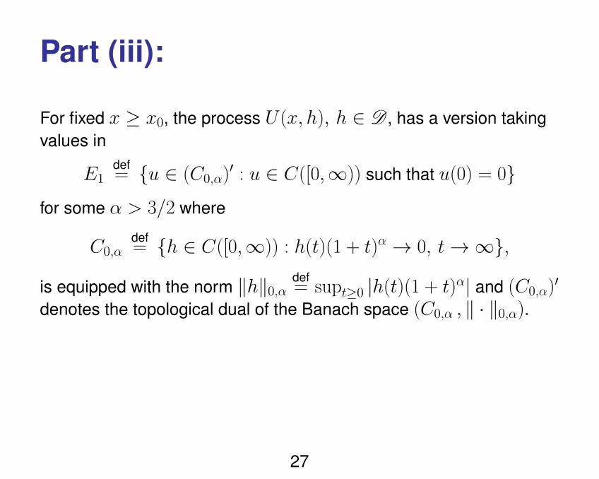
Part (iii):

For fixed x ≥ x0, the process U(x, h), h ∈ D , has a version takingvalues in

E1def= u ∈ (C0,α)′ : u ∈ C([0,∞)) such that u(0) = 0

for some α > 3/2 where

C0,αdef= h ∈ C([0,∞)) : h(t)(1 + t)α → 0, t→∞,

is equipped with the norm ‖h‖0,αdef= supt≥0 |h(t)(1 + t)α| and (C0,α)′

denotes the topological dual of the Banach space (C0,α , ‖ · ‖0,α).

27

Part (iv):

For fixed x ≥ x0, the process ∂1U(x, h); h ∈ D has a versiontaking values in

E2def= (Ha

w,β)′ for some β > 1/4

whereHa

w,β = l ∈ L2([0,∞)) : wla ∈ Hβ.Here Hβ stands for the Sobolev space of functions f ∈ L2(R) whose

Fourier transform fF satisfies ‖(1 + | · |2)β2fF‖L2(R) < ∞ and w is

a smooth weight function such that, for some ε > 0, w ≥ 1 + | · |12+εbut w = 1 + | · |12+ε outside a neighbourhood of zero.

28

Remark

The space E2 was chosen big enough to ensure that

C1/22 : L2([0,∞))→ E2 where C2h

def=

1

2√

4π| · |∗ ha

is a Hilbert-Schmidt operator.

By Sazonov’s theorem, this is needed for a meaningful state space ofa Gaussian measure.

29

Part (v):

The family of random variables (U(x, ·), ∂1U(x, ·)), x ≥ x0, is astationary process taking values in E = E1 × E2 which has anF ⊗B([x0,∞)) - measurable version.

Later this will be used to get continuous versions.

30

Cylindrical Wiener process

Wz(l)def=

∫∫Q+

B(dy, ds) (11(x0,x0+z] ⊗ l)(y, s)

for (z, l) ∈ [0,∞)×L2([0,∞)).

For fixed l ∈ L2([0,∞)) \ 0, a version of the process

Wz(l)/‖l‖L2([0,∞)), z ≥ 0,

is a standard Wiener process with respect to the filtration

F(−∞,x0+z], z ≥ 0.

31

Get from Part (i) thatfor all (x, h) ∈ [x0,∞)×D :

U(x, h)a.s.= U(x0, h) +

∫ xx0∂1U(y, h) dy

∂1U(x, h)a.s.= ∂1U(x0, h) −

∫ xx0U(y, h′) dy − Wx−x0(h).

So, if the process

x 7→ (U(x, ·), ∂1U(x, ·)) were F(−∞,x] - adapted

then one could try to establish

Markov property of this process via martingale problem

corresponding to this stochastic differential equation.

32

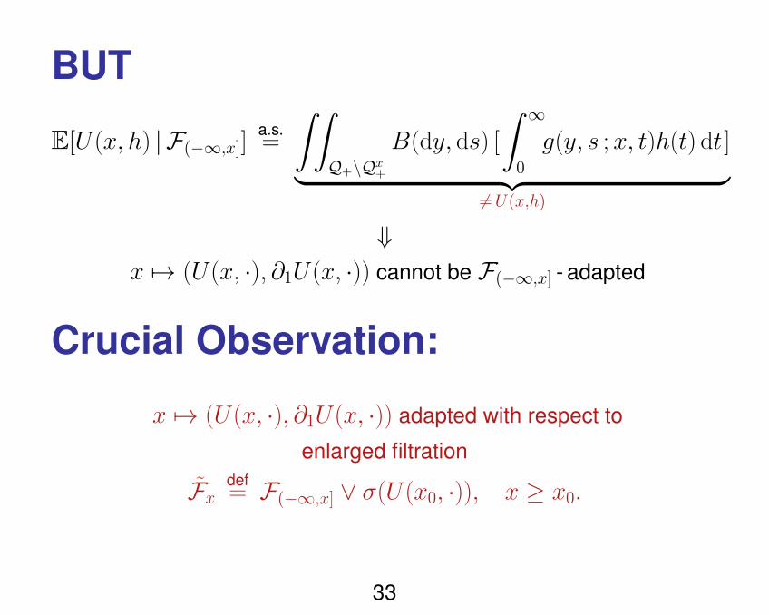
BUT

E[U(x, h) | F(−∞,x]]a.s.=

∫∫Q+\Qx+

B(dy, ds) [

∫ ∞0

g(y, s ;x, t)h(t) dt ]︸ ︷︷ ︸6=U(x,h)

⇓x 7→ (U(x, ·), ∂1U(x, ·)) cannot be F(−∞,x] - adapted

Crucial Observation:

x 7→ (U(x, ·), ∂1U(x, ·)) adapted with respect to

enlarged filtration

Fxdef= F(−∞,x] ∨ σ(U(x0, ·)), x ≥ x0.

33

However

z 7→ Wz(l) NOT Fx0+z - martingale

⇓U(x, h)

a.s.= U(x0, h) +

∫ xx0∂1U(y, h) dy

∂1U(x, h)a.s.= ∂1U(x0, h) −

∫ xx0U(y, h′) dy − Wx−x0(h).

NOT associated with martingale problem

⇓One has to find a semimartingale decomposition of the process

z 7→ Wz(l) with respect to Fx0+z, z ≥ 0.

34

ToolsAny FR - measurable random variable

L : Ω→ E, E measurable space,

is associated with an additive stochastic kernel λys(F ) indexed bybounded measurable functions F : E → R such that

F (L)a.s.= EF (L) +

∫∫Q+

B(dy, ds) λys(F ) a.s.

Let E be a Souslin locally convex topological vector space with dual E ′ and set

FC∞b (D)def= F : E → R such that F (φ) = f (h1(φ), . . . , hn(φ)) for

f ∈ C∞b (Rn), hi ∈ D, i = 1, . . . , n, n ∈ N

where D ⊆ E ′ separates the points of E.

⇓kernel λys(F ) fully described by F ∈ FC∞b (D)

35

Proposition

Fix an FR - measurable random variable L : Ω→ E andl ∈ L2([0,∞)). Assume that there exists a measurable function

%l : Ω× E × [x0,∞)→ Rsuch that

• %l(φ, y) is F(−∞,y] - measurable for each φ ∈ E and y ≥ x0;

• %l(L, y) ∈ L1(Ω) for almost every y ≥ x0;

• the mapping y 7→ %l(L, y) is in L1([x0, x]) almost surely for eachx ≥ x0;

• for each F ∈ FC∞b (D) and almost every y ≥ x0 it holds that∫ ∞0

λys(F ) l(s) dsa.s.= E

[F (L)%l(L, y)| F(−∞,y]

].

36

If

Wz(l)def= Wz(l) −

∫ x0+z

x0

%l(L, y) dy, z ≥ 0,

then, for l 6= 0, the process

Wz(l)/‖l‖L2([0,∞)), z ≥ 0,

is a standard Wiener process with respect to the filtration

F(−∞,x0+z] ∨ σ(L), z ≥ 0.

Moreover, if %l with the above properties exists for l = l1, l2 then

%a1l1+a2l2 exists for each a1, a2 ∈ Rand

Wz(a1l1 + a2l2)a.s.= a1Wz(l1) + a2Wz(l2)

for each z ≥ 0.

37

In our case:

L = U(x0, ·)

Souslin space : E1

set sepearating points of E1 : D

38

How do we get %l?

Fix y > x0 and F ∈ FC∞b (D) given by

F (φ) = f (〈φ ;h1〉, . . . , 〈φ ;hn〉), φ ∈ E1,

where f ∈ C∞b (Rn), hi ∈ D , i = 1, . . . , n, for some n ≥ 1.

⇓

Malliavin derivative DysF (U(x0, ·))

=

n∑i=1

∂if (. . . , 〈U(x0, ·) ;hi〉, . . . )∫ ∞0

g(y, s ;x0, t)hi(t) dt

Furthermore, by Clark-Ocone’s formula, we have the identity

λys(F ) = E[DysF (U(x0, ·))| F(−∞,y]

], s ≥ 0, a.s.

39

Therefore∫ ∞0

λys(F ) l(s) ds

a.s.=

n∑i=1

E[∂if (. . . , 〈U(x0, ·) ;hi〉, . . . )| F(−∞,y]

]×∫ ∞0

[

∫ ∞0

g(y, s ;x0, t)l(s) ds ]hi(t) dt

=

n∑i=1

E[∂if (. . . , 〈U(x0, ·) ;hi〉, . . . )| F(−∞,y]

]〈gx0y ∗ l0 ;hi〉

where l0def= l11(0,∞) is treated as a function on R and

gx0y (t)def=

1√4πt

exp−(x0 − y)2

4t 11(0,∞)(t), t ∈ R.

40

Above red sum of conditional expectations simplifies to∫E1

n∑i=1

∂if (. . . , 〈U(x0, ·)y ;hi〉+ 〈φy ;hi〉, . . . )〈gx0y ∗ l0 ;hi〉µy(dφy)

=

∫E1

∂Fy(φy)

∂(gx0y ∗ l0)µy(dφy)

where

U(x0, h)ydef=

∫∫Q+\Qy+

B(dy′, ds′) [

∫ ∞0

g(y′, s′ ;x0, t)h(t) dt ]

and

µy denotes the image measure of U(x0, ·)− U(x0, ·)yand

Fy(ω, φy)

def= F (U(x0, ·)y(ω) + φy).

41

But∫E1

∂Fy(φy)

∂(gx0y ∗ l0)µy(dφy) =

∫E1

Fy(φy)〈φy ;C−1y (gx0y ∗ l0)〉µy(dφy)

if the direction gx0y ∗ l0 is in the Cameron-Martin space Hy of theGaussian measure µy with covariance Cy : E ′1 → E ′′1 .

The covariance Cy : E ′1 → E ′′1 can be extended to the reproducingkernel Hilbert space H ′y of µy and Cy acts on H ′y as an isomorphismbetween H ′y and the Cameron-Martin space Hy, Hy ⊆ E1 ⊆ E ′′1 .So, checking if gx0y ∗ l0 ∈ Hy can be done by:

find a solution myl ∈ H ′y of

gx0y ∗ l0 = Cymyl .

42

If one has myl

then by the above:

∫ ∞0

λys(F ) l(s) dsa.s.=

∫E1

Fy(φy)〈φy ;my

l 〉µy(dφy)

a.s.= E

[F (U(x0, ·))〈U(x0, ·)− U(x0, ·)y ;my

l 〉∣∣F(−∞,y]

]hence, for φ ∈ E1:

%l(φ, y) = 〈φ− U(x0, ·)y ;myl 〉

43

Solution of gx0y ∗ l0 = Cymyl (heat equation):

For ν > 0, if

lνdef=

1√4π| · |

∗ (e−ν · )a

then

myν =

2√νe−ν ·

e−√ν(y−x0)

〉, y > x0,

and

%lν(U(x0, ·), y)a.s.= U(y,

√νe−ν ·) + ∂1U(y, e−ν ·), y > x0.

44

Solution of gx0y ∗ l0 = Cymyl (cable equation):

For ν > 0, if

lνdef=

ν + 1

ν

e−|·|√4π| · |

∗ (e−ν · )a − 1

ν[e− ·√π ·

11(0,∞)] ∗ [e−ν · 11(0,∞)]

then

myν =

2√ν + 1 e−ν ·

e−√ν+1(y−x0)

〉, y > x0,

and

%lν(U(x0, ·), y)a.s.= U(y,

√ν + 1 e−ν ·) + ∂1U(y, e−ν ·), y > x′0

where

gx0y (t)def=

1√4πt

exp−(x0 − y)2

4t− t 11(0,∞)(t), t ∈ R.

45

Since%lν(U(x0, ·), y)

a.s.= U(y, f (ν) e−ν ·) + ∂1U(y, e−ν ·)

want operators A1 and A2 such that

A1e−ν · = f (ν) e−ν · and A2lν = e−ν ·

leading to the new SDE

U(x, h)a.s.= U(x0, h) +

∫ x

x0

∂1U(y, h) dy

∂1U(x, h)a.s.= ∂1U(x0, h) −

∫ x

x0

[U(y, h′ + A1A2h) + ∂1U(y,A2h)] dy

− Wx−x0(h)

which gives a martingale problem w.r.t. enlarged filtration.

46

For strong Markov need

• uniqueness of martingale problem;

• right-continuous sample paths.

That’s why all the regularity stuffwas needed.

47

In case of heat equation we get:U(x, h)

a.s.= U(x0, h) +

∫ x

x0

∂1U(y, h) dy

∂1U(x, h)a.s.= ∂1U(x0, h) −

∫ x

x0

[U(y, (−∂2t )12 ha) + ∂1U(y,

√2(−∂2t )

14 ha) ] dy

− Wx−x0(h)

for all (x, h) ∈ [x0,∞)×D .

Hence, U also solves the SPDE

∂2xu + [ (−∂2

t )1/2 +√

2∂x(−∂2t )1/4 ]ua = ∂x∂tB

where ua stands for the extension of u(x, t) to (x, t) ∈ R2 which isantisymmetric in t and B is another Brownian sheet.

48