On the Stochastic Travelling Salesman Problem

for the Dubin's Vehicle

by

Sleiman M. Itani

Submitted to the Department of Electrical Engineering and ComputerScience

in partial fulfillment of the requirements for the degree of

Masters of Science in Electrical Engineering and Computer Science

at the

MASSACHUSETTS INSTITUTE OF TECHNOLOGY

June 2006

@ Massachusetts Institute of Technology 2006. All rights reserved.

A u th o r ... ...... ... .............................................Department of Electrical Engineering and Computer Science

May 12, 2006

Certified by .............Munther A. Dahleh

ProfessorThesis Supervisor

Accepted by

MASSACHUSETTS INS E.OF TECHNOLOGY

NOV O 2 20061

LIBRARIES

.1 . . .

Arthur C. SmithChairman, Department Committee on Graduate Students

BARKER

2

On the Stochastic Travelling Salesman Problem for the

Dubin's Vehicle

by

Sleiman M. Itani

Submitted to the Department of Electrical Engineering and Computer Scienceon May 12, 2006, in partial fulfillment of the

requirements for the degree ofMasters of Science in Electrical Engineering and Computer Science

Abstract

In this thesis, I solve the following problem: Given a rectangular region R in which n(n is large) targets are distributed according to some continuous or piece-wise continu-ous distribution, find the length of the optimal Stochastic Travelling Salesperson tourof a Dubin vehicle over the n targets and design an algorithm that performs withina constant factor of the optimal expected tour length. We first solve the problem forthe case when the distribution of the targets in uniform in R, and then generalizethe results to any distribution. To solve the problem, we use an already known lowerbound on the expected length of the optimal tour, and we design an algorithm thatperforms within a constant factor of that lower bound. To create the constant factoralgorithm, we first study the dynamic constraints on the Dubin vehicle to create abuilding block, and then solve an important auxiliary problem in which targets arenot allowed to be too close to each other. After creating the algorithm for the uniformdistribution scenario, we establish a lower bound for the scenario where the targetsare sampled in R according to a continuous or a piece-wise continuous distribution.We finally generalize our algorithm to the non-uniform scenario and prove that it stillperforms within a constant factor of the lower bound we proved.

Thesis Supervisor: Munther A. DahlehTitle: Professor

3

4

Acknowledgments

First and Foremost, I thank God for everything good I ever had. I thank God for

putting God, faith and a whole lot of wonderful people in my life.

After that,I would like to thank my mother Sawsan Barbir for being everything

she is, the example of distilled love, selflessness, and care in the world. If I have to

dedicate anything to anybody, it would definitely be you. I've seen what you have

gone through for me and my siblings, and I know that I can never repay you; so I

just want you to know that I appreciate everything. If it weren't for your love of

knowledge and your encouragement, this work would have never happened.

I would really like to thank Professor Munther A. Dahleh, my advisor. You were

always the bearer of good news to me, you put up with my procrastination and you

were always there when I needed you. It is also very nice to see who care about the

world make it. Hopefully someday I'll be like you.

For all of the people who touched my life and left an everlasting impression in

my character, I would like to convey my deepest and most sincere appreciation. My

dearest sister Douha and brothers Mustapha and Ibrahim, I just love you all so much

and thank you for more things than I can think of. My close friends who know me so

well they look into my soul, Taha, Abdelkader, Saif, Yahya and all of the guys from

school, I have been with you for two thirds of my life, and you were always great

brothers, perfect friends and wonderful people and for that I would like to thank you.

Mr. Saud Kawwas and Mr. Abdelraheem Hajjar, I would like to thank you for all

the things you taught me about life, dreams and myself.

My friends from AUB, who I shared the most fun days of my life with, Zaid and

Iyad, my friends with hearts of gold, Ghada, Hind and Hamza, Nabil, Antonio, Hani,

Naamani, Spiro, Wissam, Roy, Karaki, Layal, Joelle, Rani, and Rawia, a great group

with great memories, and Najwa, my wonderful younger sister, I want to thank you

all for being yourselves.

My friends from MIT, just having you guys around makes everything much better.

Even MIT wasn't so bad because you guys were here, so Costas, Demba, Erin, Aykut,

5

Danielle, Georgos, Sree, Keith, Holly and Micheal; I would like to thank you all for

being great friends through these two years.

6

Contents

1 Introduction 11

1.1 Traveling Salesperson Problem . . . . . . . . . . . . . . . . . . . . . 12

1.2 Dubin's Vehicle and Curves . . . . . . . . . . . . . . . . . . . . . . . 15

1.3 Dubins Traveling Salesperson Problem . . . . . . . . . . . . . . . . . 16

1.4 M otivation . . . . . . . . . . . . . . . . . . . . . . . . . . . . . . . . . 16

2 Background, Notation, and an Auxiliary Problem 19

2.1 Background and Notation . . . . . . . . . . . . . . . . . . . . . . . . 19

2.1.1 Optimal tour length lower bound: . . . . . . . . . . . . . . . . 19

2.1.2 Minimum distance between a point and a line under the Dubin

m etric: . . . . . . . . . . . . . . . . . . . . . . . . . . . . . . . 20

2.2 Scanning Algorithm . . . . . . . . . . . . . . . . . . . . . . . . . . . . 21

2.2.1 Algorithm Terminology and Definitions: . . . . . . . . . . . . 22

2.2.2 Algorithm Description: . . . . . . . . . . . . . . . . . . . . . . 25

2.2.3 Constant factor: . . . . . . . . . . . . . . . . . . . . . . . . . . 26

2.2.4 Bound on the expected length of the SA tour: . . . . . . . . . 30

2.2.5 Expected Tour length Bound . . . . . . . . . . . . . . . . . . 31

3 Iterated Level Algorithm 33

3.0.6 Level Algorithm Description . . . . . . . . . . . . . . . . . . . 33

3.0.7 Level Algorithm Constant Factor Guarantee: . . . . . . . . . . 36

3.0.8 Level Algorithm Expected Length . . . . . . . . . . . . . . . . 39

3.0.9 Iterating the Level Algorithm . . . . . . . . . . . . . . . . . . 40

7

3.0.10 Total Length: . . . . . . . . . . . . . . . . . . . . . . . . . . . 40

4 Non-Uniform Distributions 43

4.1 Non-Uniform Distributions . . . . . . . . . . . . . . . . . . . . . . . . 43

4.1.1 Lower Bound . . . . . . . . . . . . . . . . . . . . . . . . . . . 43

4.1.2 Iterated Level Algorithm . . . . . . . . . . . . . . . . . . . . . 45

4.1.3 Level Algorithm Constant Factor Guarantee: . . . . . . . . . . 46

4.1.4 Level Algorithm Expected Length . . . . . . . . . . . . . . . . 48

4.1.5 Total Length: . . . . . . . . . . . . . . . . . . . . . . . . . . . 48

5 Conclusion 51

5.1 Future W ork . . . . . . . . . . . . . . . . . . . . . . . . . . . . . . . . 51

8

List of Figures

2-1 Figure 1: Optimal path from a point to a straight line . . . . . . . . . 21

2-2 Figure 1: Scanning Algorithm . . . . . . . . . . . . . . . . . . . . . . 24

9

10

Chapter 1

Introduction

The Stochastic Dubins Traveling Salesperson Problem is simply the Traveling Sales-

person Problem where the vehicle (SalesPerson) has a bounded average curvature, the

cities (targets) to be visited are randomly generated and the cost to be minimized is

the expected value of the tour length. We are studying the case where the number of

cities to be visited is large. To introduce the Dubins Traveling Salesperson Problem,

we will first introduce the Traveling Salesperson Problem and study its history and

the main results related to it. We will then consider the point to point dubin curves

and their properties. The last part of this chapter contains the motivation for Dubins

Traveling Saleperson Problem.

Chapter two will introduce the notation that we will use, cite some relevent results

for the case where the distribution of the targets is uniform (including a lower bound

on the expected length of the tour) and extend them. We will then prove some facts

that we will need in the following chapters and finally solve an auxiliary problem that

is an integral element in the solution of the main problem.

Chapter three will contain the description of the Iterated Level Algorithm and the

proof that it produces a tour that has an expected length that is a constant factor of

the proven lower bound.

Chapter four will contain the generalization of both the lower bound and the Iter-

ated level Algorithm to the case where the distribution of the targets is not uniform.

11

1.1 Traveling Salesperson Problem

The Traveling Salesperson Problem is defined as follows: Given a graph of n < 00

points, find the Hamiltonian circuit that incurs the minimum cost. A Hamiltonian

circuit is a graph cycle (closed loop) that visits every node of the graph exactly once.

Here, the cost is defined as the sum of the weights of the individual edges of the

circuit, which are arbitrary positive numbers.

The Traveling Salesperson Problem, with its variations, is one of the most studied

combinatoric problems [27, 28, 29]. It is known that the TSP is an NP problem,

meaning that the best bound for the time it takes to find the solution by a known

algorithm is Q(e") when there are n targets. No efficient (polynomial time) algorithm

for solving the general or Euclidean TSP is known. Still, some instances are known

where the special structure of the graph and edges makes the problem solvable in

polynomial time [4,6,8]. The more structure that is added, the easier the problem

becomes. The Euclidean TSP is widely studied and has polynomial time algorithms

that produce a tour whose length is within (1 + E) times the shortest tour for any

E (the order of the polynomial depends on c and as c -+ 0, the algorithm becomes

exponential.) On the other hand, TSP problems with little or no structure cannot be

approximated in polynomial time [22, 23, 24, 26].

Branch and Bound:

Branch and Bound is a method for solving optimization problems. The main idea

is the following: Any optimization problem can be formulated as a search problem.

Branch and bound methods cover the space by several subregions, and then try to

eleminate some of the subregions by proving that they are not optimal. This is done

by finding easily computable lower and upper bounds for the cost in each subregion.

For a minimization problem, if we know that the lower bound for region A is greater

than the upper bound for region B then we know that the minimum is not acheivable

in A and we can disregard it in the search [10].

Cutting Plane Method:

First introduced by George Dantzig, Ray Fulkerson, and Selmer Johnson in 1954

12

[11]; this method solves consecutive linear programming relaxations of an optimization

problem to find the solution of the problem itself.

The space of tours of n cities can be mapped to the space of binary vectors of

length "(?1) by mapping every edge in the graph to an entry in the vector. A

certain tour is thus mapped to the vector that has 1 corresponding to any edge that

is included in the tour and 0 otherwise. If we designate the (n-1) vector of costs by

c, the TSP problem will then be stated as follows:

minimize cTx, where

xEX (1.1)

Where X is a complex set. A very direct linear programming relaxation of (2.1)

is:

minimize cTx where

Ax < b (1.2)

The important observation that gives the Cutting Plane Method its power is that

if we know that the solution of (1.2) is not a solution of (1.1), we know that there is

a hyperplane P between the solution of (1.2) and X. The inequality restricting us to

look on the same side of the P as X can be added to the previous set of inequalities

and thus gives us a tighter relaxation. This can be iterated to get the solution of the

original problem [12,13.

Genetic Algorithms:

Genetic Algorithms are heuristics in that they will in general result in a "good"

tour very quickly. As the name reveals, these algorithms try to mimic evolution.

Genetic algorithms rely on "the survival of the fittest", in that "crossover" between

good solutions will give a good solution. They also use "mutation" to add some

randomness in hope to find better solutions [14].

Genetic Algorithms start with an original "population", a collection of tours cre-

ated randomly in the case of TSP. A pair of parents are chosen so that they have

relatively low costs (with respect to the rest of the population) and two children

are created by "crossover"; which is a mixing of the parents that tries to make the

13

children "resemble" their parents.

If a deterministic crossover is used, then after a number of generations all of the

population will look similar, therefore random mutations are added to generate new

tours in the population.

A fact that makes genetic algorithms a bit less appealing for solving a TSP is that

good TSP tours can be extremely different and thus crossover between good tours

doesn't neccessarily result in a good tour. Some work has been done on crossover

that preserves the order [15].

Simulated Annealing:

Simulated Annealing is another heuristic that tries to mimic nature. In physics,

annealing is a process that is used to drive material to very low energy levels. What

is done is that the material is heated to a very high energy level where all the atoms

can move, and then it is slowly cooled down. It is necessary that the temperature is

lowered by small steps amd the material reaches thermal equilibrium at every step in

temperature decrease. Annealing allows materials to reach low energy levels and to

have a lot of structure when the process ends [16, 17].

A Metropolis Monte Carlo simulation is an algorithm that tries to minimize (max-

imize) a certaing function f(y) by picking a point y in the space and then trying to

move around y looking for a better solution. If moving in a certain direction results in

a better value, the move is accepted with probability 1, if it results in a worse value,

it is accepted with a probability that is exponentially decaying with the difference in

the values of the function. This means that if the initial point is yi and the second is

Y2, with f(y2) > f(yi), then the probability of moving from yi to Y2 is e-a((Y2> ;Y1))

where a is a constant.

To minimize a function f(y), Simulated Annealing uses a series of Metropolis

Monte Carlo simulations that have the constant a going from around 0 to oc. In

every step that a is changed, the best solution for the previous value of a is used as

the initial point for the Metropolis Monte Carlo simlulation for the current value of

a.

The name is used because if the constant a is set to be , where k is the Boltzman

14

constant, the algorithm will be simulating the annealing of a material that had f as

the energy.

There are a lot of other known methods for solving TSP problems, both exact

algorithms and heuristics. Nueral Networks, Dynamic Programming and Ant colonies

are some of the most popular [18, 19, 20].

1.2 Dubin's Vehicle and Curves

The Dubin's vehicle is a nonholonomic vehicle with an upper bound on its average

curvature (lower bound on its turn radius, which we will call p). It is an appropriate

model for many vehicles and robots, especially aerial and marine vehicles. The name

follows the mathematician who was the first to solve the following problem: Given

any two points pi and pj, the headings at those points Oi and Oj, and a number r; find

the shortest curve that starts at pi with a heading 0j, ends at pj with heading Oj and

has avarage curvature less than r.

Theorem 1[3]:

The optimal path for a Dubin's vehicle given the previous setting always exists and

takes one of two forms (C, C, C), (C,S, C) or any truncation of those two forms. Here,

C stands for a circular arc (clockwise or anticlockwise) whose radius is the minimum

turning radius (p), and S stand for a straight line segment.

In both forms of the Dubin's path ((C,C,C) and (C,S,C)); the first (last) curve is

a part of the cirlce of radius p that is tangent to the given heading at the first (last)

point. Two such circles can be constructed for each point, on different sides of the line

indicating the heading. One of these circles has clockwise orientation and the other

has anti-clockwise orientation so that the orientation of the circle would also match

the orientaion of the heading at the point. So, for a given pair of points, there are

four (C,S,C) curves that can be constructed to connect the points. Only two (C,C,C)

curves are possible because for a (C,C,C) curve, the orientation of the first and last

arcs has to be the same. The Dubin's curve is usually determined by trying all six

configurations and choosing the one that has the least length. There are some studies

15

that specify which path is optimal for any configuration of points and headings [9].

It is important to note that the Dubin's metric (not really a metric) becomes close to

the Euclidean metric when the points are very far away, but it has radically different

characteristics as the Euclidean distance between the points becomes comparable to

P.

1.3 Dubins Traveling Salesperson Problem

The TSP problem for the Dubin's vehicle (DTSP) is a TSP problem where the path

can be traversed by a Dubin's vehicle. This implies two requirements, the first is that

between any two points, the path taken is a Dubin's curve. The second requirement is

that the headings of the two Dubin's curves that meet at the same point are the same.

So for a fixed heading at each point, the DTSP is reduced to an asymmetric TSP

problem where the distances satisfy the triangular inequality. Finding the optimal

headings is hard, because changing the heading at one point changes the distance

from that point to all other points. This means that we have two NP problems (TSP

and minimizing a non-convex function) that are interwined. The Stochastic DTSP

problem is the problem in which the points are generated by a random process, and

the cost is the expected value of the tour length.

1.4 Motivation

The DTSP and the Stochastic DTSP are coming into the picture because of advances

in robotics and the growth of interest in Unmanned Aerial Vehicles (UAV's) [25, 30,

31]. The possible use of robots and UAV's in search and rescue missions, surveillance

and many other applications that require optimized planning of a route. The Dubin

vehicle is the natural simple model for many of those vehicles and robots, and thus

it is the appropriate model to use for path planning . Studying the DTSP and the

Stochastic DTSP might also offer insight to the solution of different problems where

there are still constraints on the curvature. This is a more general class of applications

16

that allows the cost function to be modified to account for areas of danger, priority

between customers and many other applications that seem to be dawning with the

feasibility of making commercial autonomous vehicles and robots.

Our work will mainly build on the work of Savla, Bullo and Frazzoli in (1],[2]. They

studied the same problem, established a tight lower bound and an upper bound, and

provided and algorithm that results in a tour of expected length O(n 2/3 ln((n))1 /3)1 .

So the problem that we are addressing is the following: Given a rectangle R( of area

A, hight H and width W) and n points randomly distributed in A (where n is large),

we want to find the expected optimal length of the Dubin's vehicle path through all

of the points, and an algorithm that performs close to the expected optimal length.

'We say a function f (n) is O(g(n)) if there is a c > 0 such that lim ,fn <; c (the limit could

be 0), we say f(n) is Q(g(n)) if g(n) is O(f (n)) and we say f(n) is e(g(n)) if there is a c > 0 such

thatlim_.f () = c . We say f(1) is o(l) if limjo - 0

17

18

Chapter 2

Background, Notation, and an

Auxiliary Problem

2.1 Background and Notation

In this chapter we mainly introduce the notation we will use and provide direct

extensions of previous results that are necessary for our proofs. Most of the results are

from those on the point to point Dubin vehicle problem and some related problems.

Since the Dubin curve, and thus Dubin distance, depend on the headings at each

target; a target is usually augmented with an angle and is represented in (R2, S)

where S=[0,27r] represents the angle that the heading vector at the point makes with

the x-axis.

2.1.1 Optimal tour length lower bound:

From [1], given n targets that are unifromly distributed in a region, the expected

length of the optimal TSP tour by a Dubin's vehicle over all of the points is Q(n 2/3).

For the same problem, if the vehicle does not have any dynamic constraints (it can

change directions instantaneously); then the expected length of the optimal TSP tour

is e(fn).

19

2.1.2 Minimum distance between a point and a line under

the Dubin metric:

Let a straight line L, and a Dubin vehicle with minimum turning radius p at a point

(p, #) such that the heading at p is parallel to L (if L is parallel to the x-axis, then

# = 0) . Denote the Euclidean distance from p to L (the length of the projection of p

on L) by d and the point that is the projection of p on L by p/. Denote the shortest

curve that the vehicle has to follow to go from (p, #) to L and keep moving on L by

C. The requirement that the vehicle has to keep moving on L means that C should

be tangent to L at the point of their intersection (ps). Let CI be the length of C

from p till pf and ILI the distance between p/ and p.

Proposition 1:

as d - 0, |C| < IL| + o(|L|).

This means that if a Dubin's vehicle is moving parallel to a line and close to it, it

can go onto the line and continue moving on it with almost no loss compared to the

case where the vehicle is on the line from the beginning.

Proof. To prove this proposition we will have three steps:

1. Determine C.

2. Prove that ILI = 2Vp/d - o(d).

3. Prove that 1C 5 2 pd + o(d).

The first step is a known result: If d < p; then the shortest trajectory of the

vehicle is made up of two circular arcs with radius p [5]. The first arc is tangent to

the straight line passing through p and parallel to L, the second is tangent to L and

both arcs are tangent to each other at the point of their intersection.

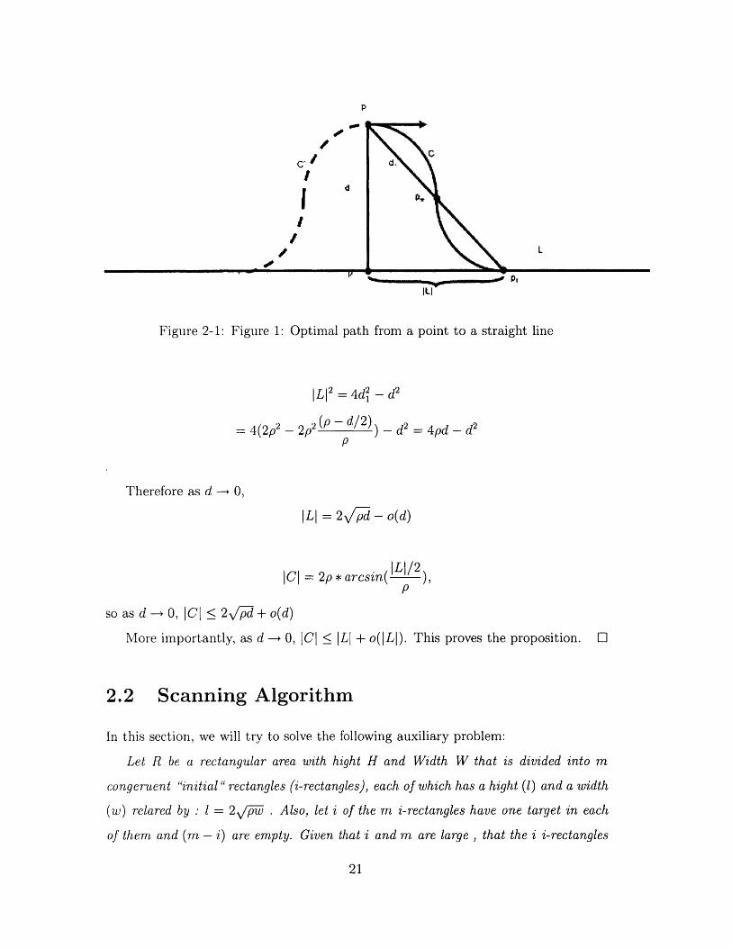
The second and third steps can be acheived by using Figure 1 and a bit of basic

geometry: Let p, be the point of intersection of the two arcs in C. By symmetry, p,

is the middle point on C between p and pf. Denote the Euclidean distance between

p and pm by di; we have the following:

20

P

/L

Figure 2-1: Figure 1: Optimal path from a point to a straight line

|L|12 = 4d 2 - d 2

1. p

4(2p 2 - 2 2 (P - d/2)) - d2 = 4pd - d2

P

Therefore as d -- 0,

ILI = 2p - o(d)

ICI = 2p * arcsin( /)

so as d -+ 0,1 C 2\/ d + o(d)

More importantly, as d -- 0, ICI < ILI + o(ILI). This proves the proposition. l

2.2 Scanning Algorithm

In this section, we will try to solve the following auxiliary problem:

Let R be a rectangular area with hight H and Width W that is divided into m

congeruent "initial" rectangles (i-rectangles), each of which has a hight (1) and a width

(w) relared by : I = 2,/pw . Also, let i of the m i-rectangles have one target in each

of them and (m - i) are empty. Given that i and m are large , that the i i-rectangles

21

with targets in them are distributed uniformly between the m i-rectangles and that the

target's location inside a non-empty i-rectangle is uniform; design an algorithm that

determines a tour for a Dubins vehicle so that it visits at least constant factor of the

i targets and has an expected tour length that is O(i2 /3 ).

We now introduce the Scanning Algorithm, which will solve the problem above.

We begin with some terminology and defenitions that will be needed in the algorithm

and bound proofs.

2.2.1 Algorithm Terminology and Definitions:

In the Scanning Algorithm, we will divide the whole rectangle R into strips. Let

k, > 0 be a parameter of the algorithm (to be determined later). The number of

strips will be The parameter ki will appear in both the constant factor(WH)

2

of the targets that the algorithm guarantees to visit and in the expected length of

the tour. The optimal value of k, will not be determined in the discussion of this

algorithm, but it will be calculated after the Scanning Algorithm is integrated in the

Iterated Level Algorithm.

With no loss of generality, the strips have been chosen to be parallel to H. After

dividing R into 2 H strips, the width of each strip will be:

_ /(WH) 2

wsVi) = (2.1)W8(i) - 2p 1/3(kii) 2 /3

We will now define some terms that we will use in the algorithm:

1. Guidance Lines:

The lines that are between the strips are called guidance lines, since the vehicle

will generally follow them. Note that the vehicle will be on the edge of any strip

twice, once on each of the guidance lines adjacent to the strip.

2. Retrieval:

We say the vehicle retrieved a target q when it leaves the guidance line, visits q

and returns to the guidance line. To do so, we chose that the vehicle will follow

22

a, path that is an extension of the curve C that was introduced earlier. This

path is made up of C, and a curve C' that is symmetrically opposite to C with

respect to d. The vehicle will follow C' to leave the guidance line and get to

the target, and will follow C to go back to the guidance line. The heading at q

is parallel to the guidance lines.

3. Cost of Retrieval:

The cost of the retrieval is the length of the path from the point the vehicle

leaves the guidance line, until it comes back to it again. It should be obvious

by now (by proposition 1) that if d < p, the cost of retrieval is almost the same

as just following the guidance line to the point where C intersects the line.

4. Scanning Area:

We define the "scanning area" of the vehicle as follows: The set of points that

belong to one of the adjacent strips and can be retrieved with a cost less than

4 /pd where d is the Euclidean distance from the point to the guidance line.

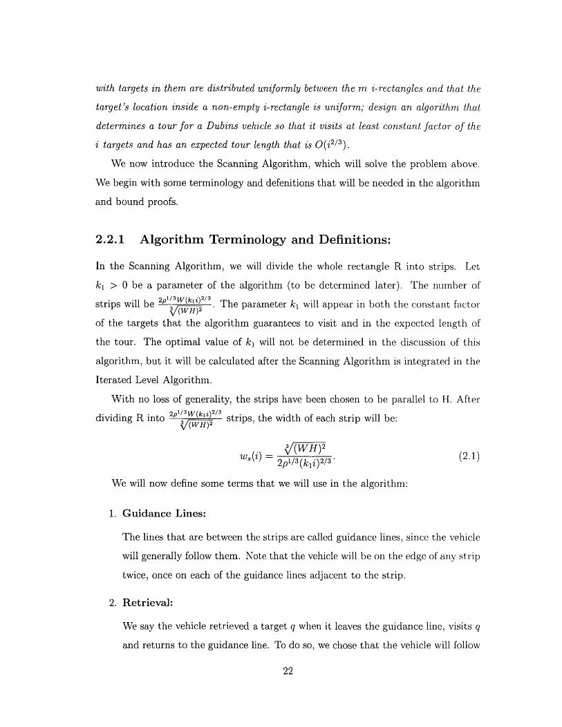
The scanning area for the vehicle at point A is shown in Figure 2.

5. Current Rectangles (c-rectangles):

the "current" rectangles (c-rectangles as opposed to the i-rectangles) that are

actually segments of the strips. Each c-rectangle has width wc(i) equal to the

width of the strips (w,(i)) and a length 1,(i) that is related to wc(i) by:

l(i) = 2 /2pwc(i)

Now, since we have from equation (2.1):

_ (WH) 2

w() 2p/3(ki)2/3

Then:

lc ( i ) 2p / 3 ( 3 'W H

23

GuidanceLines

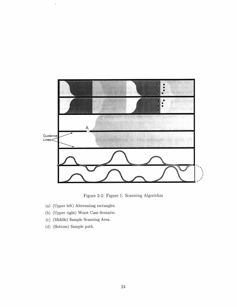
Figure 2-2: Figure 1: Scanning Algorithm

(a) (Upper left) Alternating rectangles.

(b) (Upper right) Worst Case Scenario.

(c) (Middle) Sample Scanning Area.

(d) (Bottom) Sample path.

24

and the area of each of the c-rectangles is:

_W HActi) = w,(i j1e(i) = .H

The reason we chose the c-rectangles to have these lengths and widths is simple;

they are the rectangles that contain the longest retreival the vehicle will make.

Since the vehicle will retreive targets that are in the adjacent strips of the

guidance lines, the Euclidean distance between the retreived target and the

guidance line (d in Figure 1)is less than w,(i), and this means that the horizontal

distance that the vehicle didn't travel on the guidance line (twice |LI in Figure

1) is less than 1,(i) that was calculated here. Of course, this all depends on the

assumption that i is large enough so that w,(i) < p.

2.2.2 Algorithm Description:

The scanning Algorithm can be described as follows:

We divide the area into strips that have width w,(i) and are separated by guidance

lines. The strips are numbered bottom up, and the c-rectangles are numbered left to

right in odd strips and right to left in even strips (and increasingly with the number of

the strip). The vehicle makes two similar passes. In the first (second) pass, it moves

on the guidance lines and retrieve the first target it finds that is in the scanning

area and an odd (even) numbered c-rectangle. It then continues on the guidance line

untill it finds another target that is in both the scanning area and an odd (even)

numbered c-rectangle. Each pass consists of moving on all guidance lines. In this

version of the algorithm, the vehicle moves on the guidance lines, from bottom to

top and alternating in the direction along consecutive guidance lines. As mentioned

before, the vehicle will has two chances to retreive targets from each strip, once while

moving on the guidance line below the strip and once going back on the guidance line

above the strip.

25

2.2.3 Constant factor:

lemma 1:

The Scanning Algorithm removes a constant factor of the i targets originally in

R.

Proof. The proof that the Scanning Algorithm visits at least a constant factor of the

targets has two parts:

1. Prove that each c-rectangle has at least one point with probability greater than

ci where ci is a non-zero constant (independent of m and i).

2. Prove that the Scanning Algorithm will visit at least one target in each non-

empty c-rectangle unless it has visited two from another c-rectangle. This means

that the total number of targets it visits is at least equal to the number of non-

empty c-rectangles.

Proofs:

1. Each c-rectangle is non-empty with probability greater than c1 > 0

Here, we will divide the arguemnt into two parts depending on the value of k1 .

First, we consider the case when a significant part of the area of any c-rectangle

is inside one i-rectangle. We then bound the probability that the c-rectangle is

empty by the probability that its largest intersection with any of the i-rectangles

is empty. The restriction we will use on k, is that k, ;> . Note that for the

c-rectangles, the relationship between the lengths and widths is

le(i) = 2 2pwc(i),

while for the i-rectangles, the relationship is:

I = 2 pw

26

These two equations show that if wc(i) = 2w, then 1c(i) = 21. This means that

if the Area of a c-rectangle is less than four times the Area of an i-rectangle,

then wc(i) < 2w and 1,(i) < 21.

The ratios of the area of the c-rectangles to the area of the i-rectangles is

mki i

it is enough to have k, > to guarantee that every c-rectangle can't have

more than one i-rectangle inside it.

We will prove that the probability that any c-rectangle is empty is bounded by:

(1 -rAn

There are two cases with the condition k1 > ', a c-rectangle might have an

i-rectangle totally inside it or not. If this is the case, we bound the probability

that the c-rectangle is empty by the probability that the i-rectangle inside it is

empty and this will give us the desired bound.

If a c-rectangle doesn't have any i-rectangles totally inside it, then it either

intersects four or six i-rectangles. If it intersects four, we bound the probability

that the c-rectangle is empty by the probability that its largest intersection

with one of the i-rectangles is empty. We note that the area of the largest

intersection is greater than the quarter of the area of the c-rectangle, and the

bound follows. If it intersects six i-rectangles, then there are two i-rectangle

that have their lengths or widths totally inside the length or width of the c-

rectangle. From the restriction on kj, we know that wc(i) < 2w and l(i) < 21.

We also know that the one of those two i-reactangles has to take at least half

of the other dimension. This means that we found an i-rectangle that has at

least the quarter of the area of the c-rectangle in it. Bounding the probability

that the c-rectangle is empty by the probability that that part of it is empty

will give us the desired bound.

27

We can prove the same bound for the case that k, < m. Note that in this

case, any c-rectangle is guaranteed to have at least one i-rectangle totally inside

it. The probability that a c-rectangle is empty can be upper bounded by the

probability that all the i-rectangles that are totally inside it are empty. This

gives us our desired bound of:

(4 -) i <p e-m

To find a bound that is independent of m and i, we can prove that the continuous

version of the bound,

1f W) = (I - - ) 4

x

where

x >1

is bounded by a number independent of x. To show this, we show that f(x) is

increasing with x and it is therefore bounded by

lim f(x)

Now,

g(x) = 4kidln(f(x)) ln(x - 1) - in(x) +dx x-1

g(x) > 0

since

1 1 19'(x) = X I-X -( )

x -1 x (x -1) 2

-1

x(x - 1)2

This means that g(x) is decreasing and thus

28

g(x) > lim g(x) = 0

f (x) is increasing with x since:

4k, d ln(f (x))g(x) dx

Therefore

Vx > 1, f(x) < lim f(x)X-_400

f f(X) < Cj VX

4 ( ) < e 4kM

This means that the probability of a c-rectangle to be non-empty

than 1 - e~k.

Therefore, the Scanning Algorithm is guaranteed to remove at least

k,(1 - e~Y) of the targets.

is not less

a factor of

2. The Scanning Algorithm will remove at least one target from each non-empty

c-rectangle

This is true because of the design of the c-rectangles. In each pass, we will

remove targets from alternating c-rectangles. Note that for the c-rectangle that

we are "skipping" we have 1,(i) = 2 2pw0(i), which is the maximum "retreival

cost" possible. This means that the vehicle is able to go back to the guidance

line and come back and pick any target from the following rectangle.

We thus proved that the Scanning Algorithm will remove at least a constant factor

of the targets initially in R.

29

2.2.4 Bound on the expected length of the SA tour:

Lemma 2:

The maximum distance traveled in any pass of the guidance lines is less than:

W H+Wc1 1WH +Wc,+ H + C2 + 0( )wS(i W /w 8-(i)

Proof. First, we will start by finding the distance traveled when crossing one guidance

line: For a certain pass on one of the guidance lines in which we retrieve k targets,

we denote the the retreival cost (as defined before) of the jth target by Lj and the

distance on the guidance line that was skipped by the retreival by I. We have:

k

El j + If < H.j=1

Where l is the distance travelled on the guidance line. We also have, because of the

assumption that i is large (w,(i) < p):

Vi,

Lj lj + o(w,(i)).

Thereforek

Z Lj +lf f H +o(Vw,(i)).j=1

The reason the last term is o(rw 8(i)) can be shown by proving that the longest

pass will be when ( )) points are retrieved and the distance to each of them from

the guidance line is wc(i). The total length will therefore be of o( w,(i)).

Therefore the distance travelled in traversing one guidance line is bounded by

DGL =H + o( w,(i)).

To turn from one guidance line to the other, an additional distance bounded by

Dturn c1 + w,(i) is needed; where ci < 2.6587rp [2].

30

The number of guidance lines is

WNg < + 1

_ w 8(i)

To go back to the beginning of first guidance line, we must travel at most the

diagonal of the square and some distance for changing direction. This total distance

is bounded by

c2 = v -W2 + H 2 + c 1 .

Thus the total distance travelled in one loop over the whole square is bounded by:

Ng[DGL + Dturn] + C2

which is equal to:

WH±Wc1H(_1WH +Wc,+ H + c2 + o(7 )w8(i) ywn

2.2.5 Expected Tour length Bound

The length of the distance travelled by the vehicle following the Scanning Algorithm

is bounded by two times the maximum distance travelled in any certain pass over the

guidance lines.

Therefore for large i and from Lemma 1 and the fact that

- (W H) 2

wi)=2pi/3(kii)2/3

WH+Wc1 1DSA < 2 +0 )

-- w8(i) w8(i)

S(WH + Wc 1)(2p 1/3) (kii)2/3I(WH)2

31

Therefore, the Scanning Algorithm visits a constant factor of the i targets in

O(i 2/ 3).

The auxiliary problem and the Scanning Algorithm will play a major role in our

solution for the DTSP. In the following chapter, we introduce the Iterated Level Algo-

rithm, which produces a tour for the Stochastic Dubins Traveling Salesman Problem

and will use the Scanning Algorithm as a module. We will prove that the tour created

by the Iterated Level Algorithm is a constant factor of the known lower bound [1]

and thus prove that the SDTSP is 8(n2/3).

32

Chapter 3

Iterated Level Algorithm

In this Chapter, we will solve the followin problem: Given n targets that are uniformly

distributed in a rectangle R that had width W and height H; design an algorithm for

a Dubin's vehicle that will allow it to visit all of the n targets so that the expected

length of the tour is O(n 2/3).

Here, we will present the Iterated Level Algorithm that will have a performance

within a constant factor of the established lower bound. To do that, we will create

an 0(n2 /3) algorithm (the Level Algorithm) that removes a constant factor of the

targets while keeping the distribution of the remaining targets distributed in a way

that will allow the Level Algorithm to be iterated. This algorithm can be iterated till

the remaining number of targets is less than V/i and the remaining targets will be

removed using any algorithm that is O(f). We will first present the Level Algorithm

and then prove the necessary bound on the produced tour's expected length. We will

then prove that the distribution of the remaining targets at the end of the Level

Algorithm will allow us to iterate it. The bounds on the Expected length of the

Iterated Level Algorithm will follow.

3.0.6 Level Algorithm Description

The Level Algorithm will be our solution to the following problem:

Given :

33

A rectangular area R that is divided into identical i-rectangles (the same i-

rectangles in the Scanning Algorithm), and that the random variable representing

the number of targets in each i-rectangle has a Poisson distribution with the same

parameter (k2 ) for all the i-rectangles. The distribution of targets in non-empty i-

rectangles is uniform and the number of targets in any i-rectangle is independent of

the number of targets in any other i-rectangle.

Required:

Design an Algorithm for a Dubin's vehicle, so that the Algorithm produces a path

that allows the vehicle to retreive a constant factor of the targets, such that the length

of the path is O(n 2/3 ) when there are n targets, and such that the distribution can

be bounded by a uniform distribution of cn targets where c < 1 is a constant.

The Level Algorithm has Three steps:

1. Initialization step: Divide the whole area into i-rectangles (the ones introduced

in the Scanning Algorithm). Number the targets in each of the i-rectangles

and create "levels", which are collections of targets that have the same number

(from different i-rectangles).

2. Pre-procesing step: Remove all targets from levels that have a few targets (to

be determined later).

3. Level processing step: Trace the non-empty levels top-down and at each level,

apply the Scanning Algorithm.

Initialization:

Here, we will choose the parameter k2. We will study the performance of the

algorithm for any k, and k2 , and in the end we will choose k, and k2 to minimize the

bound on the expected tour length.

In the initialization step, we first divide the area into the i-rectangles, each with

width w 1 3 (2n)2/

3 and length I = _2 n)(/ 3 . We randomly number the

targets in each i-rectangle. Targets from different i-rectangles that have the same

number will form a "level". We think of each i-rectangle as a stack, and the targets

34

in it as elements on top of each other in the stack, ordered by the numbers we gave

them. It is useful to imagine the area A now as a histogram, where above every

i-rectangle there is a stack that contains the targets in that i-rectangle. It is obvious

that a. lower level cannot contain less targets than any of those above it.

We will study the probability distribution of X, the random variable indicating

the number of points in any one of the i-rectangles, as n -4 oo. X has a binomial

distribution of n trials and probability of success -. This means that, as n -+ 00:n

p.d.f.(X) -4 Piosson(n * kn

Poisson(k2)

Therefore the probability that the number of points in a certain i-rectangle is i is

given by:e-k2ki

P(X =i)= -2i!

In fact, the Level Algorithm doesn't need the assumption of uniform distribution,

it only needs the assumption that the distribution of X is a poisson and the same for

all i-rectangles. We will prove that when the Level Algorithm is applied, the targets

that are left will satisfy these assumptions.

Pre-procesing:

The reason pre-processing is needed is that in the Scanning Algorithm, we assumed

that the number of targets is large. If the area of the rectangles is large (their number

is small), the bounds that we have proved will not hold. We therefore need to clear

all levels that have a small number of targets (less than n'/ 2).

Doing this is actually not dificult at all, since we know that the number of levels

is less than ln(n) almost surely. This means that the total number of targets in all

levels that have less than n1/2 is less than ni1 / 2 ln(n). Therefore, they can all be cleared

using a tour that has a tour length that is O(ni1 /2 ln(n)).

Level Processing:

The algorithm passes over each of the remaining levels once . When processing

35

any level, we only consider the targets in that level and apply the Scanning Algorithm

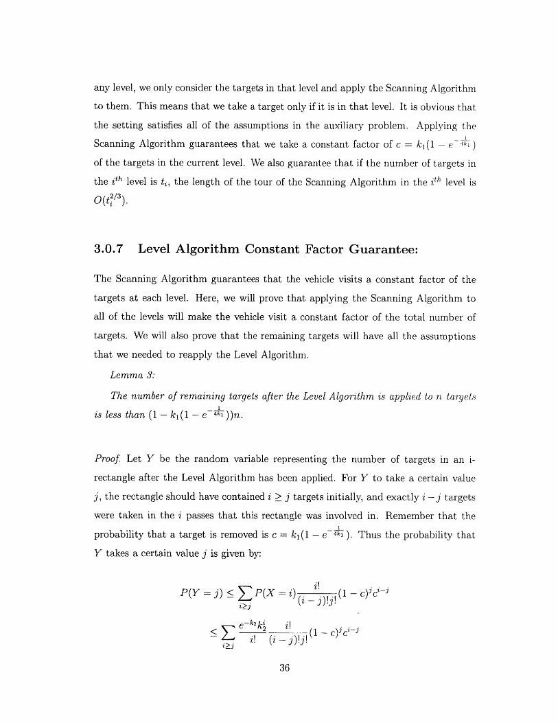
to them. This means that we take a target only if it is in that level. It is obvious that

the setting satisfies all of the assumptions in the auxiliary problem. Applying the

Scanning Algorithm guarantees that we take a constant factor of c = k (1 - e- 4)

of the targets in the current level. We also guarantee that if the number of targets in

the ith level is ti, the length of the tour of the Scanning Algorithm in the ith level is

O(t2/'3

3.0.7 Level Algorithm Constant Factor Guarantee:

The Scanning Algorithm guarantees that the vehicle visits a constant factor of the

targets at each level. Here, we will prove that applying the Scanning Algorithm to

all of the levels will make the vehicle visit a constant factor of the total number of

targets. We will also prove that the remaining targets will have all the assumptions

that we needed to reapply the Level Algorithm.

Lemma 3:

The number of remaining targets after the Level Algorithm is applied to n targets

is less than (1 - k1 (1 - e i ))n.

Proof. Let Y be the random variable representing the number of targets in an i-

rectangle after the Level Algorithm has been applied. For Y to take a certain value

j, the rectangle should have contained i > j targets initially, and exactly i - j targets

were taken in the i passes that this rectangle was involved in. Remember that the

probability that a target is removed is c = k, (1 - e- 4). Thus the probability that

Y takes a certain value j is given by:

P(Y = j) P(X = i) -(1 - c)1c'-1

-k2k' IE 1 2 -. (t - C)3c -

36

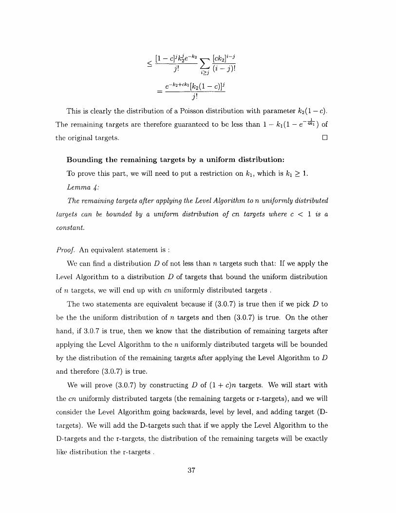
[1 - c]ik2e-k2 [ck 2]i3

e-k2+ck2 [k 2 (1 - C)]j

j!

This is clearly the distribution of a Poisson distribution with parameter k2 (1 - c).

The remaining targets are therefore guaranteed to be less than 1 - ki(1 - e 4k) of

the original targets. D

Bounding the remaining targets by a uniform distribution:

To prove this part, we will need to put a restriction on kj, which is k, > 1.

Lemma 4:The remaining targets after applying the Level Algorithm to n uniformly distributed

targets can be bounded by a uniform distribution of cn targets where c < 1 is a

constant.

Proof. An equivalent statement is

We can find a distribution D of not less than n targets such that: If we apply the

Level Algorithm to a distribution D of targets that bound the uniform distribution

of n targets, we will end up with cn uniformly distributed targets .

The two statements are equivalent because if (3.0.7) is true then if we pick D to

be the the uniform distribution of n targets and then (3.0.7) is true. On the other

hand, if 3.0.7 is true, then we know that the distribution of remaining targets after

applying the Level Algorithm to the n uniformly distributed targets will be bounded

by the distribution of the remaining targets after applying the Level Algorithm to D

and therefore (3.0.7) is true.

We will prove (3.0.7) by constructing D of (1 + c)n targets. We will start with

the cn uniformly distributed targets (the remaining targets or r-targets), and we will

consider the Level Algorithm going backwards, level by level, and adding target (D-

targets). We will add the D-targets such that if we apply the Level Algorithm to the

D-targets and the r-targets, the distribution of the remaining targets will be exactly

like distribution the r-targets .

37

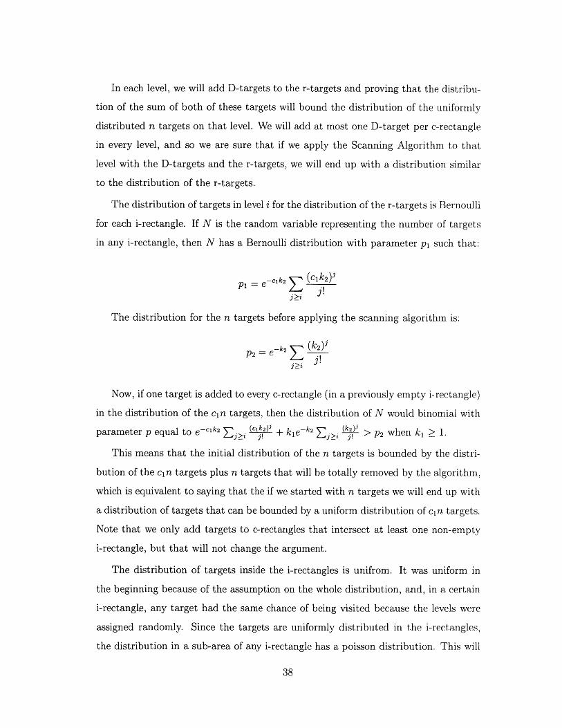
In each level, we will add D-targets to the r-targets and proving that the distribu-

tion of the sum of both of these targets will bound the distribution of the uniformly

distributed n targets on that level. We will add at most one D-target per c-rectangle

in every level, and so we are sure that if we apply the Scanning Algorithm to that

level with the D-targets and the r-targets, we will end up with a distribution similar

to the distribution of the r-targets.

The distribution of targets in level i for the distribution of the r-targets is Bernoulli

for each i-rectangle. If N is the random variable representing the number of targets

in any i-rectangle, then N has a Bernoulli distribution with parameter pi such that:

P1 = e-c1k2 E (c 1 k2 )j

The distribution for the n targets before applying the scanning algorithm is:

P2 = ek2 E (k 2 )j

Now, if one target is added to every c-rectangle (in a previously empty i-rectangle)

in the distribution of the c1in targets, then the distribution of N would binomial with

parameter p equal to e-cik2 Z (clk2)j + kie-k2 i () > P2 when k1 ; 1.

This means that the initial distribution of the n targets is bounded by the distri-

bution of the c1in targets plus n targets that will be totally removed by the algorithm,

which is equivalent to saying that the if we started with n targets we will end up with

a distribution of targets that can be bounded by a uniform distribution of cin targets.

Note that we only add targets to c-rectangles that intersect at least one non-empty

i-rectangle, but that will not change the argument.

The distribution of targets inside the i-rectangles is unifrom. It was uniform in

the beginning because of the assumption on the whole distribution, and, in a certain

i-rectangle, any target had the same chance of being visited because the levels were

assigned randomly. Since the targets are uniformly distributed in the i-rectangles,

the distribution in a sub-area of any i-rectangle has a poisson distribution. This will

38

allow us to bound the distribution of the number of targets in the i-rectangles of the

next iteration. LI

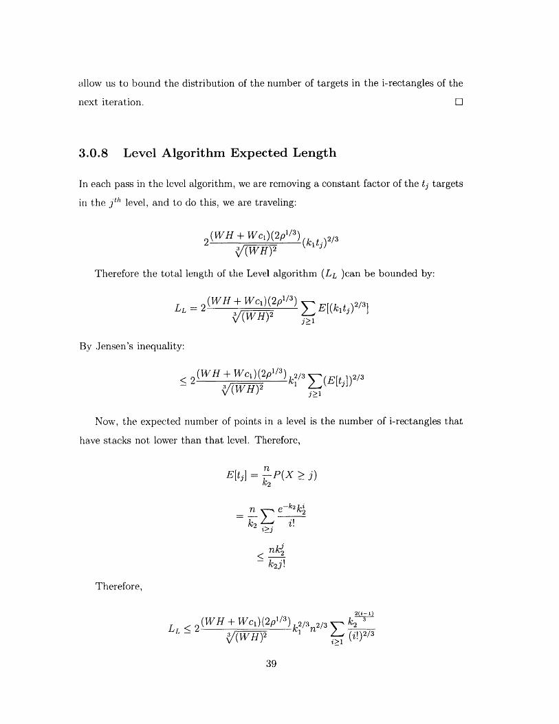
3.0.8 Level Algorithm Expected Length

In each pass in the level algorithm, we are removing a constant factor of the t, targets

in the J t level, and to do this, we are traveling:

2 (WH + Wc1 )(2p'/ 3) (kitj)2/3

T(W H) 2

Therefore the total length of the Level algorithm (LL )can be bounded by:

(WH + Wcl)(2p'/ 3)L = 2 (WH)2 E E[(klt )2/3]

By Jensen's inequality:

< 2(WH + Wcj)(2pl/ 3) k2 / 3 \(E[tj]) 2/3

<(WH)2 1

Now, the expected number of points in a level is the number of i-rectangles that

have stacks not lower than that level. Therefore,

E[tj] = nP(X;> j)

n ek2ki

k2 i

nko

k2 j!

Therefore,

L L 2 (W ±H + Wcl)(2p/3) k2/3n2/3L ( (W H)2 1 E

2(i-1)

k2 3

(j!)2/3

39

< 2(WH + Wc1)(2p 1/ 3 ) k1 2/3 2/ 3 k2_3

(WH)2 k2 (i!)2/3

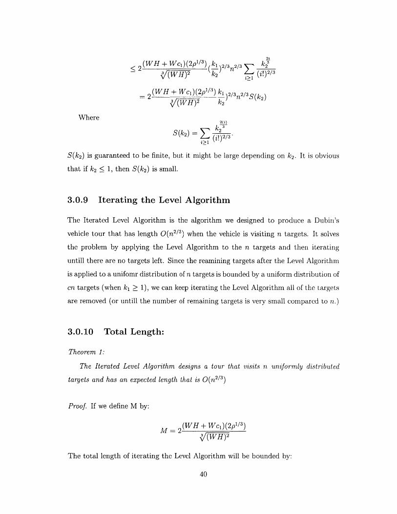
- 2 (WH + Wci)(2p 1/ 3) ki 2 /3n2 / 3 S(k 2)I(WH)2 k2

Where

S(k2)=Z k23

i>1

S(k 2) is guaranteed to be finite, but it might be large depending on k2 . It is obvious

that if k2 < 1, then S(k 2) is small.

3.0.9 Iterating the Level Algorithm

The Iterated Level Algorithm is the algorithm we designed to produce a Dubin's

vehicle tour that has length O(n 2/3 ) when the vehicle is visiting n targets. It solves

the problem by applying the Level Algorithm to the n targets and then iterating

untill there are no targets left. Since the reamining targets after the Level Algorithm

is applied to a unifomr distribution of n targets is bounded by a uniform distribution of

cn targets (when ki > 1), we can keep iterating the Level Algorithm all of the targets

are removed (or untill the number of remaining targets is very small compared to n.)

3.0.10 Total Length:

Theorem 1:

The Iterated Level Algorithm designs a tour that visits n uniformly distributed

targets and has an expected length that is O(n 2/3)

Proof. If we define M by:

M - 2 (WH + Wc1)(2p1 /3){|(W H) 2

The total length of iterating the Level Algorithm will be bounded by:

40

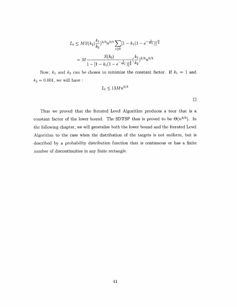
Lt _ MS(k 2 ) )2/ 3n2 /3 [ - ki(1 - e )]i>O

= M S(k 2) k1 2/3 n2/ 3

1 - [1 - ki(1 - e 4k1)]3 k2

Now, k, and k2 can be chosen to minimize the constant factor. If ki = 1 and

k2 = 0.001, we will have

Lt < 13Mnr2 / 3

Thus we proved that the Iterated Level Algorithm produces a tour that is a

constant factor of the lower bound. The SDTSP thus is proved to be e(n 2/3). In

the following chapter, we will generalize both the lower bound and the Iterated Level

Algorithm to the case when the distribution of the targets is not uniform, but is

described by a probability distribution function that is continuous or has a finite

number of discontinuities in any finite rectangle.

41

42

Chapter 4

Non-Uniform Distributions

4.1 Non-Uniform Distributions

To generalize the study to the case of non-uniform distributions, we will find a lower

bound smimilar to the one for the uniform distributions and generalize the Iterated

level algorithm for the case of non-uniform distributions.

4.1.1 Lower Bound

In this section, we will find a lower bound for the SDTSP when the distribution of the

targets has a probability distribution function f(.) that is continuous or has finitely

many discontinuities and is bounded.

This proof was used by J.J. Enright and E. Frazzoli in an unpublished paper to

find the lower bound for the uniform case. Here we generalize their proof.

Similar to the case of the uniform distribution, we will find the lower bound by

bounding the expected distance to the nearest target from any point x where f(x) > 0.

To lower bound the expected distance to the nearest target (from any target), we

find area of the set of targets that can be reached with length less than J.

We know from [9] that the area of that set R 6 is less than A- + o(63) as 6 -+ 0.3p

The probability that the distance to the nearest target is more than 6 is the same as

the probability that all targets are outside R5. If 6m is the distance to the nearest

43

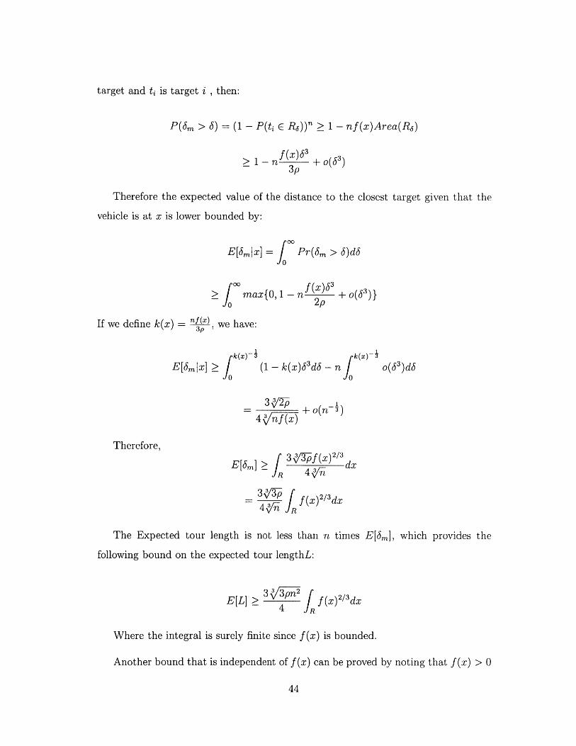
target and t. is target i , then:

P(6m > 6) = (1 - P(t G R6 ))' > 1 - nf (x)Area(R6 )

> n - n + o(63)3p

Therefore the expected value of the distance to the closest target given that the

vehicle is at x is lower bounded by:

E[6mx] = j Pr(6m > 6)d6

max{O, 1 - nf(x 3 +o(633)0O 2p

If we define k(x) = nf(x), we have:3p

k(x)-1E [6mlx] > 10 (1 - k(x)j 3 dJ - n I k(x)0

o(6 3)d6

3, 2- 1=+ O(n3)

43 nf(x)

Therefore,

/[rn 3 N3pf (X) 2/3 dE[6m] > 1 x dx

3=Nk f(x) 2/ 3dx

The Expected tour length is not less than n times E[6m], which provides the

following bound on the expected tour lengthL:

E[L] ;> 3 /3pn 2

4JR f(X)

2 3 dx

Where the integral is surely finite since f(x) is bounded.

Another bound that is independent of f(x) can be proved by noting that f(x) > 0

44

-

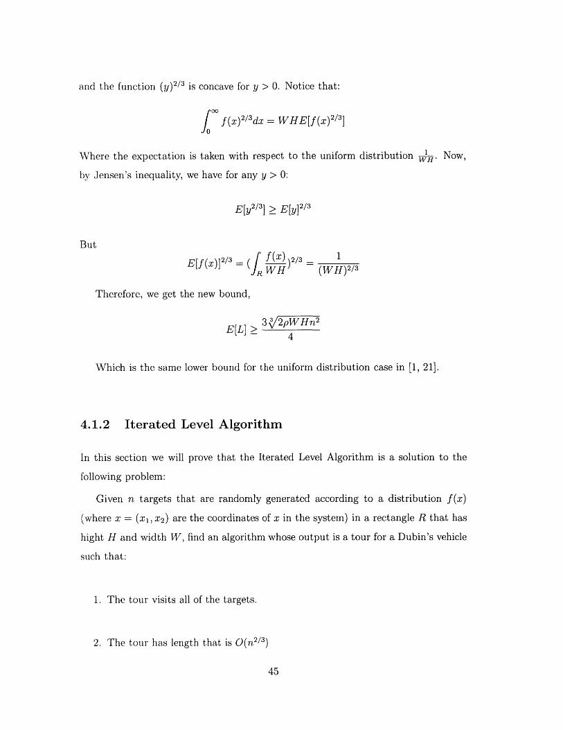
and the function (y) 2/3 is concave for y > 0. Notice that:

I00f (x) 213 dx = WHE[f (x)21 3]

o0

Where the expectation is taken with respect to the uniform distribution 1. Now,

by Jensen's inequality, we have for any y > 0:

E[y 2 /3] E[y] 2/3

But

E[f(X)]2/3 f(x)2/3 =

JR WH (WH)2/3

Therefore, we get the new bound,

EL 33/2pW Hrn2E[L] > 2 pW 24

Which is the same lower bound for the uniform distribution case in [1, 21].

4.1.2 Iterated Level Algorithm

In this section we will prove that the Iterated Level Algorithm is a solution to the

following problem:

Given n targets that are randomly generated according to a distribution f(x)

(where x = (x 1 , x 2 ) are the coordinates of x in the system) in a rectangle R that has

hight H and width W, find an algorithm whose output is a tour for a Dubin's vehicle

such that:

1. The tour visits all of the targets.

2. The tour has length that is O(n2/ 3)

45

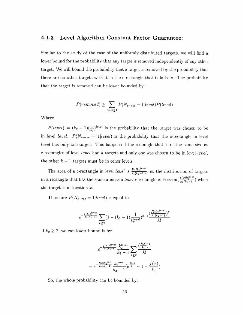
4.1.3 Level Algorithm Constant Factor Guarantee:

Similar to the study of the case of the uniformly distributed targets, we will find a

lower bound for the probability that any target is removed independently of any other

target. We will bound the probability that a target is removed by the probability that

there are no other targets with it in the c-rectangle that it falls in. The probability

that the target is removed can be lower bounded by:

P(removed) > P(N-rec = I|level)P(level)level>1

Where

P(level) = (k2 - 1)(-L)level is the probability that the target was chosen to be

in level level. P(Nc-rec = 1level) is the probability that the c-rectangle in level

level has only one target. This happens if the rectangle that is of the same size as

c-rectangles of level level had k targets and only one was chosen to be in level level,

the other k - 1 targets must be in other levels.

The area of a c-rectangle in level level is kilkv)n so the distribution of targets

in a rectangle that has the same area as a level c-rectangle is Poisson( kj~2Q) when

the target is in location x.

Therefore P(Nc-rec = 1|level) is equal to:

f~level 1 f(x)k2evei)k

e k2 Z(1 - (k 2 - 1)kkive )

k>2 2

If k2 > 2, we can lower bound it by:

f(x)k 1ev el k level (f(WX)k

e k1 (k2 -I) k 2 1 k!k2 - 1 k>2 k

l~~kevel k fevlx))x= e k1 (k2 -1) 2 l(e k-1 -

k2 - w ki

So, the whole probability can be bounded by:

46

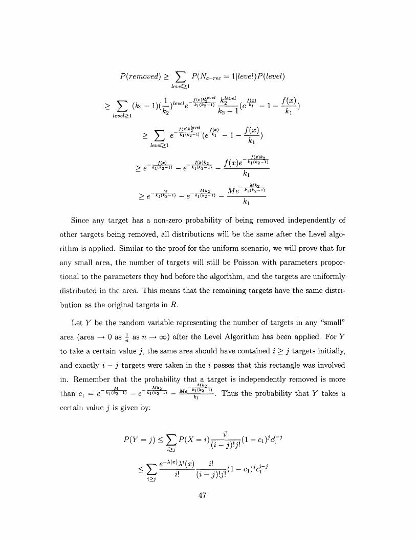
P(removed) P(Nerec = IIlevel)P(level)level>1

f (.T)k level k level X> ( - k) ()level e1 (k2-1) 2 e f _W

level >1 k2 k2 ~ ki

>f(x)klevel f(x) f(X)S el~k1(e kj -1- )level>1

f(x)k2

f(x) _ f(x)k f(x)e-k(k21)> e kI(k 2 -1) - e ki(k2-1) -k

Mk 2

M Mk A e k 1 (k 2 -1)

> ek(k2-1) - e k1 (k 2 -1 -

- ki

Since any target has a non-zero probability of being removed independently of

other targets being removed, all distributions will be the same after the Level algo-

rithm is applied. Similar to the proof for the uniform scenario, we will prove that for

any small area, the number of targets will still be Poisson with parameters propor-

tional to the parameters they had before the algorithm, and the targets are uniformly

distributed in the area. This means that the remaining targets have the same distri-

bution as the original targets in R.

Let Y be the random variable representing the number of targets in any "small"

area (area - 0 as 1 as n -- oc) after the Level Algorithm has been applied. For Yn

to take a certain value j, the same area should have contained i > j targets initially,

and exactly i - j targets were taken in the i passes that this rectangle was involved

in. Remember that the probability that a target is independently removed is moreM _Mk _TMk9

than ci = e- kiki) - - kI (k2 1- Me I(k2-0). Thus the probability that Y takes a

certain value j is given by:

P(Y -j< P(X -i) . (1- CI) 3c Z

e-)(x) i - c

i~ .i! (i - ( )

47

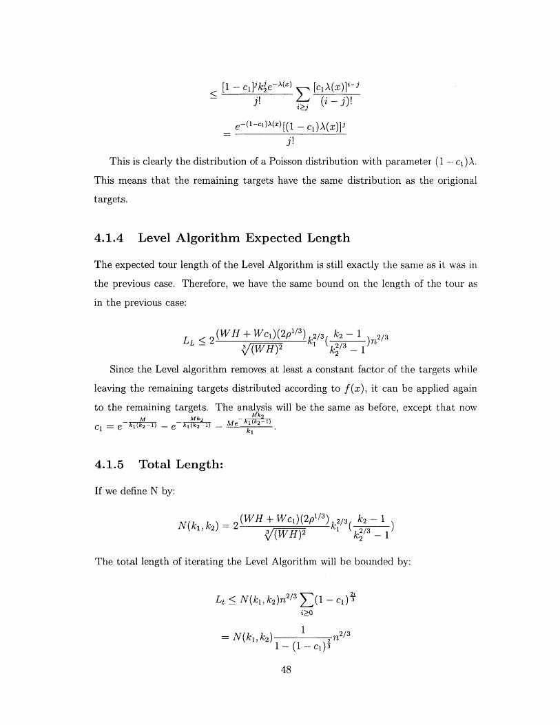
[1 - ci]ik2e-A(x) [ciA(x)]~3(i -- i)!

e-( 1 c1)A(x) [(1 - ci)A(x)]j

This is clearly the distribution of a Poisson distribution with parameter (1 - ci)A.

This means that the remaining targets have the same distribution as the origional

targets.

4.1.4 Level Algorithm Expected Length

The expected tour length of the Level Algorithm is still exactly the same as it was in

the previous case. Therefore, we have the same bound on the length of the tour as

in the previous case:

(WH + Wc 1)(2p/ 3 ) /3 k2 - 1 2/3LL <2 (WH)2 k 2/3 _ )2

Since the Level algorithm removes at least a constant factor of the targets while

leaving the remaining targets distributed according to f(x), it can be applied again

to the remaining targets. The analysis will be the same as before, except that now- Mk 2

Mk2

Ci = e k1(k2-1) - e - ki(k2 -1> -1) " (k2-1)

4.1.5 Total Length:

If we define N by:

(WH + Wcl)(2p/ 3 ) k2/3 k 2 - 1N(k1, k2 ) 2 ( )2 k1 (

(W H )2 k2/

The total length of iterating the Level Algorithm will be bounded by:

Lt <; N(k1 , k2 )nr2/ 3 Z(1 - Cii>O

1 2/=N(k, k 2 ) 2 2/3

1 - (1 -c

48

-2 (WH + Wcl)(2p'1/3) k2/3( k2 - 1 1 n 2/3

(WH)2 2/3 1 - (1 - - eki 2 1 _M e k1 2->

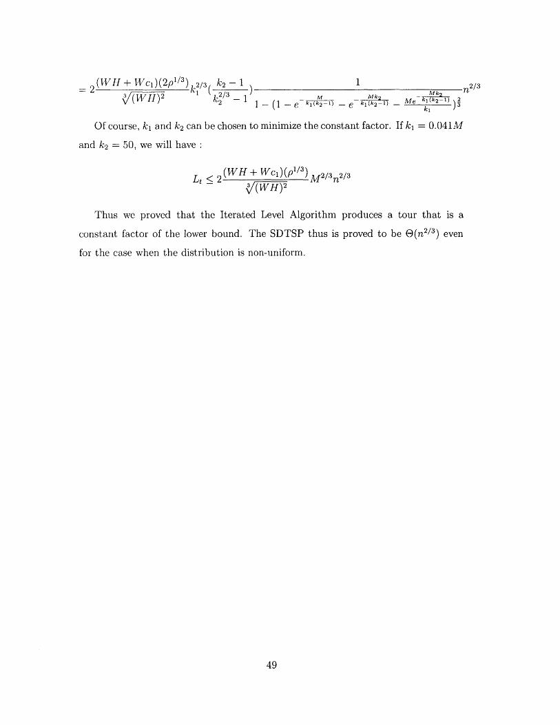
Of course, k, and k2 can be chosen to minimize the constant factor. If ki = 0.041M

and k2 = 50, we will have :

Lt < 2(WH + Wcl)(p'/3) M2/3n2/3L/(WH)

2

Thus we proved that the Iterated Level Algorithm produces a tour that is a

constant factor of the lower bound. The SDTSP thus is proved to be 8(n2/3) even

for the case when the distribution is non-uniform.

49

50

Chapter 5

Conclusion

In this thesis, we studied the Stochastic DTSP, proved that the expected length of the

optimal tour is 1(n 2/ 3 ). To do that we provided a lower bound that is Q(n 2/3 ) and

an algorithm that produces a tour that has and expected length that is O(n 2 / 3). The

algorithm we provided is novel, efficient and most importantly simple and elegant. It

is simple because although the Dubin's vehicle has dynamic constraints that make the

problem much harder, we used the large number of points and the structure imposed

by the Dubin's vehicle to our advantage. The simplicity of the algorithm will make

generalizations possible. It is a polynomial time algorithm and thus as efficient as

possible for an approximation algorithm for the DTSP.

We then generalized both the lower bound and the study of the algorithm to the

case of the non-uniform distribution, and we proved that also in that case the expected

optimal tour length of the SDTSP is 9(n 2 / 3). The lower bound we provided for this

case is 0(n2/3 ), but it was different from the uniform case in that it depended on the

probability distribution function of the targets, and we generalized the Iterated Level

Algorithm so that it provides a tour that has an expected length that is O(n 2/ 3).

5.1 Future Work

In the future, we might use the results here to study the DTRP, where the TRP is

the traveling repairsman problem introduced by Bertsimas and Van Ryzin in 1991

51

[7]. The DTSP and DTRP in the non-uniform case were never studied due to their

complexity compared to the uniform case, we hope that our study here will provide

help for us in handling those problems. Usually, the solution for the Stochasic TSP

provides stability conditions for the DTRP problem with the same constraints, this

fact is what we hope to use in our future study of the DTRP.

52

Bibliography

[1] K. Savla, F. Bullo, and E. Frazzoli. "On Traveling Salesperson Problems for

Dubins' vehicle: stochastic and dynamic environments". In Proc. IEEE Conf.

on Decision and Control, December 2005.

[2] K. Savla, E. Frazzoli, and F. Bullo. "On the point-to-point and traveling

salesperson problems for Dubins' vehicles." In Proc. of the American Control

Conference, 2005.

[3] L. E. Dubins, On Curves of minimal length with a constraint on average

curvature and with prescribed initial and terminal positions and tangents,

American Journal of Mathematics, vol. 79, pp. 497-516,1957.

[4] D. Applegate, R. Bixby, V. Chv4atal, and W. Cook, "On the solution of trav-

eling salesman problems," in Documenta Mathematica Journal der Deutschen

Math ematiker- Vereinigung, (Berlin, Germany), pp. 645-656, Aug 1998. Pro-

ceedings of the International Congress of Mathematicians, Extra Volume ICM

III.

[5] Erzberger, H., and Lee, H.Q.,"Optimum Horizontal GuidanceTechniques for

Aircraft," Journal of Aircraft, Vol. 8 (No. 2), pp. 95-101, February, 1971.

[6] J. Bearwood, J. Halton, and J. Hammersly, "The shortest path through many

points," in Proceedings of the Cambridge Philosophy Society, vol. 55, pp. 299-

327, 1959.

53

[7] D.J. Bertsimas and G.J. Van Ryzin, "A stochastic and dynamic vehicle routing

problem in the Euclidean plane," Operations Research, vol. 39, pp. 601-615,

1991.

[8] S. Arora, "Nearly linear time approxation scheme for Euclidean TSP and

other geometric problems," in Proceedings of 38th IEEE Annual Symposium

on Foundations of Computer Science, (Miami Beach, FL,) pp. 554-563, Oct.

1997.

[9] Bui X. et. Al, "Shortest Path Synthesis for Dubins Non-holonomic Robot,"

IEEE 1994

[10] A. H. Land and A. G. Doig, "An Automatic Method for Solving Discrete

Programming Problems Econometrica", Vol.28 (1960), pp. 497-520.

[11] G. B. Dantzig, R. Fulkerson, and S. M. Johnson, "Solution of a large-scale

traveling salesman problem", Operations Research 2 (1954), 393-410.

[12] M. W. Padberg and M. Grtschel, "Polyhedral computations", The Traveling

Salesman Problem (E. L. Lawler et al., eds.), Wiley, Chichester, 1995, pp.307-

360.

[13] M. W. Padberg and G. Rinaldi, "A branch-and-cut algorithm for the resolu-

tion of large-scale symmetric traveling salesman problems", SIAM Review 33

(1991), pp. 60-100.

[14] P. Moscato, "On Genetic Crossover Operators for Relative Order Preserva-

tion" ,Caltech Concurrent Computation Program C3P report 778.

[15] V.M. Kureichik, V.V. Miagkikh, and A.P. Topchy, "Genetic Algorithm for

Solution of Traveling Salesman Problem with New Features agains Premature

Convergence"

[16] 0. Martin and S.W. Otto, "Combining Simulated Annealing with Local Search

Heuristics".

54

[17] Rachel Moldover and Paul Coddington, "Improved Algorithms for Global Op-

timization" 54.

[18] A. Ossen, "Learning Topology Preserving Maps Using Self-Supervised Back-

propagation on a Parallel Machine", TR-92-059, International Computer Sci-

ence Institute, Berkley, CA September 1992.

[19] M. Dorigo, V. Maniezzo, and A. Colorni, "The Ant System: Optimization by

a, Colony of Cooperating Systems", IEEE transactions on Systems, Man, and

Cybernetics-Part B, 26, 1, 29-41, 1996.

[20] T. Stotzle and Holger Hoos, "The MAX-MIN Ant System and Local Search

for the Traveling Salesman Problem", ICEC 1997.

[21] J. J. Enright and E. Frazzoli, "UAV routing in a stochastic time-varying envi-

ronment", IFA C World Congress, (Prague, Czech Republic), July 2005. Elec-

tronic Proceedings.

[22] S. Arora. "Polynomial time approximation schemes for euclidian traveling

salesman and other geometric problems". Journal of the ACM, 45(5):753-782,

1998.

[23] S. Lin and B. W. Kernighan," An effective heuristic algorithm for the traveling-

salesman problem", Operations Research, vol. 21, pp. 498-516, 1973.

[24] C. H. Papadimitriou. "Euclidian TSP is NP-complete". Theoretical Computer

Science, 4:237-244, 1977.

[25] Z. Tang and U. Ozguner, "Motion planning for multi-target surveillance with

mobile sensor agents", IEEE Transactions on Robotics, Jan. 2005.

[26] J. M. Steele, "Probabilistic and worst case analyses of classical problems of

combinatorial optimization in Euclidean space"; Mathematics of Operations

Research, vol. 15, no. 4, p. 749, 1990.

55

[27] N. Christofides. "Worst-case analysis of a new heuristic for the travelling sales-

man problem". Technical report, CSIA, Carnegie-Mellon Univ., 1976.

[28] A. Frieze, G. Galbiati, and F. Maffioli. "On the worst-case performance of

some algorithms for the asymmetric traveling salesman problem". Networks,

12:23-39, 1982.

[29] C.E. Noon and J.C. Bean. "An efficient transformation of the generalized

traveling salesman problem". Information Systems and Operational Research,

31(1), 1993.

[30] A. M. Shkel and V. J. Lumelsky,"Classification of the Dubins set", Robotics

and Autonomous Systems, vol. 34, pp. 179-202, 2001.

[31] P. Jacobs and J. Canny. "Planning smooth paths for mobile robots". Non-

holonomic Motion Planning (Z. Li and J. Canny) , pages 271-342. Kluwer

Academic, 1992.

56