on the structure of isometries between noncommutative lp spaces
TRANSCRIPT

Publ. RIMS, Kyoto Univ.4x (200x), 000–000
On the structure of isometries betweennoncommutative Lp spaces
By
David Sherman ∗
Abstract
We prove some structure results for isometries between noncommutative Lp
spaces associated to von Neumann algebras. We find that an isometry T : Lp(M1)→Lp(M2) (1 ≤ p < ∞, p 6= 2) can be canonically expressed in a certain simpleform whenever M1 has variants of Watanabe’s extension property. Although theseproperties are not fully understood, we show that they are possessed by all “approx-imately semifinite” (AS) algebras with no summand of type I2. Moreover, when M1
is AS, we demonstrate that the canonical form always defines an isometry, resultingin a complete parameterization of the isometries from Lp(M1) to Lp(M2). AS al-gebras include much more than semifinite algebras, so this classification is strongerthan Yeadon’s theorem (and its recent improvement), and the proof uses independenttechniques. Related to this, we examine the modular theory for positive projectionsfrom a von Neumann algebra onto a Jordan image of another von Neumann alge-bra, and use such projections to construct new Lp isometries by interpolation. Somecomplementary results and questions are also presented.
§1. Introduction
In any class of Banach spaces, it is natural to ask about the isometries.(Here an isometry is always assumed to be linear, but not assumed to besurjective.) Lp function spaces are an obvious example, and their isometrieshave been understood for half a century. To the operator algebraist, theseclassical Lp spaces arise from commutative von Neumann algebras, and onemay as well ask about isometries in the larger class of noncommutative Lp
Communicated by H. Okamoto. Received May 18, 2004. Revised November 5, 2004.2000 Mathematics Subject Classification(s): Primary 46L52; Secondary 46B04Key Words: von Neumann algebra, noncommutative Lp space, isometry, Jordan *-homomorphism∗Department of Mathematics, University of California, Santa Barbara, CA 93106, USA.
c© 2004 Research Institute for Mathematical Sciences, Kyoto University. All rights reserved.

2 David Sherman
spaces. This question was considered by a number of authors, with a varietyof assumptions; a succinct answer for semifinite algebras was given in 1981by Yeadon [Y1]. In the recent paper [JRS], Yeadon’s result was extended tothe case where only the initial algebra is assumed semifinite. We will callthis the Generalized Yeadon Theorem (GYT) (Theorem 2.2 below), as it wasproved there by a simple modification of Yeadon’s original argument. With noassumption of semifiniteness, the author classified all surjective isometries inthe paper [S1]. But in its most general form, the classification of isometriesbetween noncommutative Lp spaces is still an open question.
Let us agree that “Lp isometry” will mean an isometric map T : Lp(M1) →Lp(M2), 1 ≤ p < ∞, p 6= 2. Adapting Watanabe’s terminology ([W2], [W3]),we say that an Lp isometry is typical if there are
1. a normal Jordan *-monomorphism J : M1 →M2,
2. a partial isometry w ∈M2 with w∗w = J(1), and
3. a (not necessarily faithful) normal positive projection P : M2 → J(M1),
such that
(1.1) T (ϕ1/p) = w(ϕ ◦ J−1 ◦ P )1/p, ∀ϕ ∈ (M1)+∗ .
(Writing the projection as P : M2 → J(M1) will always mean that P fixesJ(M1) pointwise.) Here ϕ1/p is the generic positive element of Lp(M1); seebelow for explanation. Since any Lp element is a linear combination of fourpositive ones, (1.1) completely determines T . We will see in Section 2 thattypical isometries follow Banach’s original classification paradigm for (classical)Lp isometries, and may naturally be considered “noncommutative weightedcomposition operators”.
Question 1.1. Is every Lp isometry typical?
Results in the literature offer evidence for an affirmative answer. GYTand the structure theorem for L1 isometries (due to Kirchberg [Ki]) imply thatan Lp isometry with semifinite domain must be typical. In [S1] typicality wasproved for surjective Lp isometries. And the paper [JRS] shows typicality forLp isometries which are 2-isometries at the operator space level, with J actuallya homomorphism and P a conditional expectation.
Our strategy here is the following. First we use a theorem of Bunce andWright [BW1] to prove a variant of Kirchberg’s result which shows that L1
isometries are typical. Then given an Lp isometry, we try to form an associated

Lp isometries 3
L1 isometry, apply typicality there, and deduce typicality for the original map.It is not clear whether this procedure can work in general; it requires thatcontinuous homogeneous positive bounded functions on Lp(M1)+ which areadditive on orthogonal elements must in fact be additive. This is a naturalvariant of the extension property (EP) introduced by Watanabe [W2], so wecall it EPp.
We will call a von Neumann algebra “approximately semifinite” (AS) ifit can be paved out by a net of semifinite subalgebras (see Section 5 for theprecise definition). The main results of Sections 3 through 5 are summarizedin
Theorem 1.2.
1. All L1 isometries are typical.
2. An Lp isometry must be typical if M1 has EPp and EP1; for positive Lp
isometries EP1 is sufficient.
3. An AS algebra with no summand of type I2 has EPp for any p ∈ [1,∞).
4. The class of AS algebras includes all semifinite algebras, all hyperfinitealgebras and factors of type III0 with separable predual, and others.
This is a stronger result than GYT, and the proofs are independent ofYeadon’s paper. At this time we do not know any factor other than M2 whichdoes not have EPp, although we do have examples of non-AS algebras. Furtherinsight into these properties may help to resolve Question 1.1, and they seemto merit investigation in their own right.
The converse of Question 1.1 is also interesting.
Question 1.3. For a given normal Jordan *-monomorphism J : M1 →M2 and normal positive projection P : M2 → J(M1), does (1.1) extendlinearly to an Lp isometry?
If J(M1) is a von Neumann algebra, then P is a conditional expectationand the answer to Question 1.3 is yes. The construction, given in Section 6,is not entirely new, at least when J is multiplicative. In our context the keyobservation is the independence from the choice of reference state. Then inSection 7 we remove the assumption that J(M1) is a von Neumann algebra.We are able to construct new Lp isometries from the data J, P by interpolation,but now they do seem to depend on the choice of reference state. However, inSection 8 we show that the possible dependence is removed, and Question 1.3

4 David Sherman
can again be answered affirmatively, if P factors through a conditional expecta-tion from M2 onto J(M1)′′. Exactly this issue was addressed in a recent workof Haagerup and Størmer [HS2], although in a more general setting. We extendtheir investigation in our specific case, guaranteeing the necessary factorizationwhenever M1 is AS. Combining this with Theorem 1.2, we acquire a completeparameterization of the isometries from Lp(M1) to Lp(M2) whenever M1 isAS.
EP was proposed as a tool for Lp isometries by Keiichi Watanabe, and Ithank him for making his preprints available to me. With his permission, a fewof his unpublished results are incorporated here into Theorem 5.3 (and clearlyattributed to him). I am also grateful to each of Marius Junge, Zhong-JinRuan, and Quanhua Xu for helpful conversations and for showing me Theorem5.8 from [JRX].
This work was completed while the author was VIGRE Visiting AssistantProfessor at the University of Illinois at Urbana-Champaign.
§2. History and background
It is not plausible to review the theory of noncommutative Lp spaces atlength here. The reader may want to consult [Te1], [N], [K1], [Ya] for detailsof the constructions mentioned below; [PX] also includes an extensive bibli-ography. Our interest, aside from refreshing the reader’s memory, lies largelyin setting up convenient notation and explaining why “typical” isometries area natural generalization of previous results going back to the origins of thesubject.
In fact the fundamental 1932 book of Banach [B, IX.5] already listed thesurjective isometries of `p and Lp(0, 1), p 6= 2. In the second case, an Lp
isometry T is uniquely decomposed as a weighted composition operator:
(2.1) T (f) = h · (f ◦ ϕ) = (sgn h) · |h| · (f ◦ ϕ),
where h is a measurable function and ϕ is a measurable (a.e.) bijection of[0, 1]. Clearly |h| is related to the Radon-Nikodym derivative for the changeof measure induced by ϕ. Although Banach did not prove this classification,he did make the key observation that isometries on Lp spaces must preservedisjointness of support; i.e.
(2.2) fg = 0 ⇐⇒ T (f)T (g) = 0.
We will see that the equations (2.1) and (2.2) provide a model for all succeedingclassifications.

Lp isometries 5
The extension to non-surjective isometries on general (classical) Lp spaceswas made in 1958 by Lamperti [L]. His description was similar, but he notedthat generally the bijection ϕ must be replaced by a “composition” inducedby a set-valued mapping, called a regular set isomorphism. See [L] or [FJ]for details; for many measure spaces [HvN] one can indeed find a (presumablymore basic) point mapping. As Lamperti pointed out, (2.2) follows from acharacterization of equality in the Clarkson inequality. That is,
(2.3) ‖f + g‖pp + ‖f − g‖pp = 2(‖f‖pp + ‖g‖pp) ⇐⇒ fg = 0.
This method also works for some other function spaces ([L], [FJ]).It is interesting to note how much of the analogous noncommutative ma-
chinery was in place at this time. First observe that from the operator algebraicpoint of view a regular set isomorphism is more welcome than a point mapping,being a map on the projections in the associated L∞ algebra. In terms of this(von Neumann) algebra, equation (2.2) tells us that the underlying map be-tween projection lattices preserves orthogonality. Dye [D] had studied exactlysuch maps in the noncommutative setting a few years before, showing that theygive rise to normal Jordan *-isomorphisms. And Kadison’s classic paper [Ka]had demonstrated the correspondence between normal Jordan *-isomorphismsand isometries. Noncommutative Lp spaces were around, too, but the isometrictheory would wait for noncommutative formulations of (2.3).
Let us recall the definition of the noncommutative Lp space (1 ≤ p < ∞)associated to a semifinite algebra M equipped with a given faithful normalsemifinite tracial weight τ (simply called a “trace” from here on). The earliestconstruction seems to be due to Segal [Se]. Consider the set
{T ∈M | ‖T‖p , τ(|T |p)1/p <∞}.
It can be shown that ‖ · ‖p defines a norm on this set, so the completion is aBanach space, denoted Lp(M, τ). It also turns out that one can identify ele-ments of the completion with unbounded operators; to be specific, all the spacesLp(M, τ) are subsets of the *-algebra of τ -measurable operators M(M, τ) [N].Clearly τ is playing the role of integration.
Before stating Yeadon’s fundamental classification for isometries of semifi-nite Lp spaces, we recall that a Jordan map on a von Neumann algebra is a*-linear map which preserves the operator Jordan product x•y , (1/2)(xy+yx).(We denote this by • instead of ◦ since we use the latter for composition veryfrequently.) The unfamiliar reader may be comforted to know that a normalJordan *-monomorphism from one von Neumann algebra into another is the

6 David Sherman
sum of a *-homomorphism π and a *-antihomorphism π′, where s(π)+s(π′) ≥ 1and π(1) ⊥ π′(1) [St1]. (We use s and its variants s`, sr for “(left/right) supportof” throughout the paper.) This is frequently misinterpreted in the literature.Part (but not all) of the confusion comes from the fact that the image is typi-cally not multiplicatively closed; the simplest example is
J : M2 →M4, x 7→(x 00 xt
),
where t is the transpose map. Accordingly, we will refer to a Jordan image of avon Neumann algebra as a “Jordan algebra” in order to remind the reader thatit is closed under the Jordan product and not the usual product. This slightlyabusive terminology should cause no confusion; we will not need the abstractdefinitions of Jordan algebras, JW-algebras, etc.
Theorem 2.1. [Y1, Theorem 2] A linear map
T : Lp(M1, τ1) → Lp(M2, τ2)
is isometric if and only if there exists
1. a normal Jordan *-monomorphism J : M1 →M2,
2. a partial isometry w ∈M2 with w∗w = J(1), and
3. a positive self-adjoint operator B affiliated with M2 such that the spec-tral projections of B commute with J(M1), s(B) = J(1), and τ1(x) =τ2(BpJ(x)) for all x ∈M+
1 ,
all satisfying
(2.4) T (x) = wBJ(x), ∀x ∈M1 ∩ Lp(M1, τ1).
Moreover, J,B, and w are uniquely determined by T .
Note the striking resemblance between (2.1) and (2.4) - again, B is relatedto a (noncommutative) Radon-Nikodym derivative.
Traciality is essential in the construction of Lp(M, τ), so another methodis required for the general case. We proceed by analogy: if M is supposed tobe a noncommutative L∞ space, the associated L1 space should be the predualM∗. This is not given as a space of operators, so it is not clear where the pthroots are. Later, in Section 6, we will discuss Kosaki’s interpolation method[K1]. Here we recall the first construction, due to Haagerup ([H1],[Te1]), which

Lp isometries 7
goes as follows. Choose a faithful normal semifinite weight ϕ on M. Thecrossed product M , Moσϕ R is semifinite, with canonical trace τ and trace-scaling dual action θ. Then M∗ can be identified, as an ordered vector spaceand as an M−M bimodule, with the τ -measurable operators T affiliated withM satisfying θs(T ) = e−sT . We may simply transfer the norm to this setof operators, and we denote this space by L1(M). Of course, because of theidentification with M∗, L1(M) does not depend (up to isometric isomorphism)on the choice of ϕ.
We will use the following intuitive notation: for ψ ∈ M+∗ , we also denote
by ψ the corresponding operator in L1(M)+. (In the original papers thiswas written as hψ, but several other notations are in use – it is ∆ψ,ϕ ⊗ λ inthe crossed product construction of the last paragraph. Some advantages andapplications of our convention, called a modular algebra, are demonstrated in[C4, Section V.B.α], [Ya], [FT], [JS], [S2].) Recall that x ∈ M and ψ ∈ M∗
are said to commute if the functionals xψ = ψ(·x) and ψx = ψ(x·) agree. Ofcourse this is nothing but the requirement that x ∈ M ⊂ M and ψ ∈ L1(M)commute as operators. We also have the useful relations
ϕitψ−it = (Dϕ : Dψ)t; ψitxψ−it = σψt (x)
for ϕ,ψ ∈M+∗ , s(ϕ) ≤ s(ψ), x ∈ s(ψ)Ms(ψ).
Now we set Lp(M) (1 ≤ p < ∞) to be the set of τ -measurable operatorsT for which θs(T ) = e−s/pT , and defining a norm ‖T‖p = ‖|T |p‖1/p1 gives us aBanach space. As a space of operators, Lp(M) is still ordered, and any elementis a linear combination of four positive ones. This all agrees with our previousconstruction in case M is semifinite: the identification is
(2.5) Lp(M, τ)+ 3 h↔ (τhp)1/p ∈ Lp(M)+.
(Here τh(x) , τ(hx); more generally ϕh(x) , ϕ(hx) = ϕ(xh) whenever ϕ andh commute.) But the reader should appreciate the paradigm shift: now L1
elements are “noncommutative measures”. Any theory for functorially produc-ing Lp spaces from von Neumann algebras (i.e. without arbitrarily choosinga base measure) is forced into such a construction, as von Neumann algebrasdo not come with distinguished measures unless the algebra is a direct sum oftype I or II1 factors. It is more correct to think of a von Neumann algebra asdetermining a measure class (in the sense of absolutely continuity), and thisgenerates an Lp space of measures directly. See [S2] for more discussion.
Now we revisit Theorem 2.1. The operator B commutes with J(M1), andso when M1 is finite, the linear functional ϕ , |T (τ1/p
1 )|p = (τ2)Bp commutes

8 David Sherman
with J(M1). (Equivalently, the restriction of ϕ to J(M1)′′ is a finite trace.)Formulated in this way, Theorem 2.1 extends to the case where M2 is notassumed semifinite (and M1 is not assumed finite). The result, which we callGYT for “Generalized Yeadon Theorem”, was also noted in [JRS] but will beproven here as Theorem 5.6.
Theorem 2.2. [JRS] Let M1,M2 be von Neumann algebras, τ a fixedtrace on M1, and 1 ≤ p < ∞, p 6= 2. If T : Lp(M1, τ) → Lp(M2) is anisometry, then there are, uniquely,
1. a normal Jordan *-monomorphism J : M1 →M2,
2. a partial isometry w ∈M2 with w∗w = J(1), and
3. a normal semifinite weight ϕ on M2, which commutes with J(M1)′′ andsatisfies s(ϕ) = J(1), ϕ(J(x)) = τ(x) for all x ∈ (M1)+,
all satisfying
(2.6) T (x) = wϕ1/pJ(x), ∀x ∈M1 ∩ Lp(M1, τ).
Remark 2.3. An operator interpretation of τ and ϕ requires a little moreexplanation when they are unbounded functionals ([Ya],[S2]), or one can rewrite(2.6) as
(2.7) T (h1/p) = w(ϕJ(h))1/p, h ∈M1 ∩ L1(M1, τ)+,
and extend by linearity. We will use (2.7) in the sequel.
For Theorems 2.1 and 2.2, a key ingredient of the proofs is the equalitycondition in the Clarkson inequality for noncommutative Lp spaces. Yeadon[Y1] showed this for semifinite von Neumann algebras; a few years later Kosaki[K2] proved it for arbitrary von Neumann algebras with 2 < p < ∞; and onlyrecently Raynaud and Xu [RX] obtained a general version (relying on Kosaki’swork). It plays a role in this paper as well.
Theorem 2.4. [RX] (Equality condition for noncommutative Clarksoninequality)
For ξ, η ∈ Lp(M), 0 < p <∞, p 6= 2,
(2.8) ‖ξ + η‖p + ‖ξ − η‖p = 2(‖ξ‖p + ‖η‖p) ⇐⇒ ξη∗ = ξ∗η = 0.

Lp isometries 9
We remind the reader that Lp elements have left and right support pro-jections in M. Since s`(ξ) ⊥ s`(η) ⇐⇒ ξ∗η = 0 as elements of Haagerup’s Lp
space, we will call pairs satisfying the conditions of (2.8) orthogonal. (This canbe interpreted in terms of Lp/2-valued inner products, see [JS].) We mentionedearlier that isometries of classical Lp spaces preserve disjointness of support:Theorem 2.4 tells us that all Lp isometries actually preserve orthogonality,which is disjointness of left and right supports.
Comparing (1.1) and (2.1), one sees that typical Lp isometries correspondto a noncommutative interpretation of Banach’s classification result for Lp(0, 1).One may think of the partial isometry w as a “noncommutative function of unitmodulus” (corresponding to sgn h), and the precomposition with J−1 ◦ P asa “ noncommutative isometric composition operator” (corresponding to f 7→|h| · (f ◦ ϕ)).
§3. L1 isometries
The starting point for our investigation is the following (paraphrased) re-sult of Bunce and Wright. Recall that an o.d. homomorphism (M1)∗ → (M2)∗is a linear homomorphism which is positive and preserves orthogonality betweenpositive functionals.
Theorem 3.1. ( ∼ [BW1, Theorem 2.6]) If T : (M1)∗ → (M2)∗ is ano.d. homomorphism, then the map
J : s(ϕ) → s(T (ϕ)), ϕ ∈ (M1)+∗
is well-defined and extends to a normal Jordan *-homomorphism. We haveT ∗(1) central in M1, and
(3.1) T (ϕ)(J(x)) = ϕ(T ∗(1)x), ∀x ∈M1, ∀ϕ ∈ (M1)+∗ .
Consider the case where T is a positive isometry of (M1)∗ into (M2)∗.Then T is an o.d. homomorphism, as the equality condition of the Clarksoninequality shows:
ϕ ⊥ ψ ⇒ ‖ϕ+ ψ‖+ ‖ϕ− ψ‖ = 2(‖ϕ‖+ ‖ψ‖)⇒ ‖T (ϕ) + T (ψ)‖+ ‖T (ϕ)− T (ψ)‖ = 2(‖T (ϕ)‖+ ‖T (ψ)‖)⇒ T (ϕ) ⊥ T (ψ).
Applying Theorem 3.1 and equation (3.1), we first note that
(3.2) ‖ϕ‖ = ‖T (ϕ)‖ = T (ϕ)(s(T (ϕ))) = T (ϕ)(J(s(ϕ))) = ϕ(T ∗(1)s(ϕ))

10 David Sherman
for each ϕ ∈ (M1)∗, which is only possible if J is a monomorphism and T ∗(1) =1. By (3.1) we have that T ∗ ◦ J = idM1 . Then P , J ◦ T ∗ is a normal positiveprojection from M2 onto J(M1), T ∗ = J−1 ◦ P , and T is (J−1 ◦ P )∗.
The following observation will be useful. Since P = J ◦ T ∗, the supportsof P and T ∗ are the same. But s(T ∗) is the smallest projection in M2 suchthat for all x ∈ (M2)+, ϕ ∈ (M1)+∗ ,
T (ϕ)(x) = ϕ(T ∗(x)) = ϕ(T ∗(s(T ∗)xs(T ∗))) = T (ϕ)(s(T ∗)xs(T ∗)).
Thus
(3.3) s(P ) = s(T ∗) = supϕs(T (ϕ)) = sup
ϕJ(s(ϕ)) = J(1) = P (1).
Now consider an isometry T from L1(M1) to L1(M2) which is not neces-sarily positive. Let ϕ,ψ ∈ (M1)+∗ be arbitrary, and let the polar decompositionsbe
T (ϕ) = u|T (ϕ)|; T (ψ) = v|T (ψ)|; T (ϕ+ ψ) = w|T (ϕ+ ψ)|.
So u∗u = s(|T (ϕ)|), and similarly for the others. Then
|T (ϕ+ ψ)| = w∗T (ϕ+ ψ) = w∗(T (ϕ) + T (ψ)) = w∗u|T (ϕ)|+ w∗v|T (ψ)|.
View both sides as linear functionals and evaluate at 1:
|T (ϕ+ ψ)|(1) = |T (ϕ)|(w∗u) + |T (ψ)|(w∗v) ≤ |T (ϕ)|(u∗u) + |T (ψ)|(v∗v)
= ‖T (ϕ)‖+ ‖T (ψ)‖ = ‖ϕ‖+ ‖ψ‖ = ‖ϕ+ ψ‖ = ‖T (ϕ+ ψ)‖ = |T (ϕ+ ψ)|(1).
Apparently the inequality is an equality, which implies by Cauchy-Schwarz thatw s(|T (ϕ)|) = u, w s(|T (ψ)|) = v. It follows that any partial isometry occurringin the polar decomposition of some T (ϕ) is a reduction of a largest partialisometry w, with sr(w) = ∨{sr(T (ϕ)) | ϕ ∈ (M1)+∗ }, so that T (ϕ) = w|T (ϕ)|for any ϕ ∈ (M1)+∗ . Then ξ 7→ w∗T (ξ) is a positive linear isometry, and we mayuse the previous argument to obtain the decomposition T (ξ) = w(J−1 ◦P )∗(ξ).Necessarily by (3.3) w∗w = J(1); if there is a faithful normal state ρ on M1,w occurs in the polar decomposition of T (ρ).
We have shown that
Theorem 3.2. An L1 isometry is typical.
A different proof of this can be found in Kirchberg [Ki, Lemma 3.6].

Lp isometries 11
Remark 3.3. Using GYT and Theorem 3.2, it is not difficult to provethat all Lp isometries with semifinite domain are typical. For if (2.7) holds,one may define the positive L1 isometry
T ′ : τx 7→ ϕJ(x), x ∈ L1(M1, τ)+
and deduce typicality for T from that of T ′. As the development of this paperis intended to be independent of GYT, we derive this fact (and GYT) formallyin Section 5.
§4. Lp isometries, p > 1
Now consider an Lp isometry T with 1 < p <∞, p 6= 2. Define
T : Lp(M1)+ → Lp(M2)+, T (ϕ1/p) = |T (ϕ1/p)|.
Is this map linear on Lp(M1)+? To attack this question, we make the following
Definition 4.1. A continuous finite measure (c.f.m.) on Lp(M)+(1 ≤ p <∞) is a nonnegative real-valued function ρ which satisfies
1. ρ(λϕ1/p) = λρ(ϕ1/p),
2. ϕ ⊥ ψ ⇒ ρ(ϕ1/p + ψ1/p) = ρ(ϕ1/p) + ρ(ψ1/p),
3. ρ(ϕ1/p) ≤ C‖ϕ1/p‖ for some C <∞ (denote by ‖ρ‖ the least such C),
4. ϕ1/pn → ϕ1/p ⇒ ρ(ϕ1/p
n ) → ρ(ϕ1/p),
for ψ,ϕ, ϕn ∈M+∗ , λ ∈ R+.
A von Neumann algebra M will be said to have EPp (extension propertyfor p) if every c.f.m. ρ on Lp(M)+ is additive. This implies that ρ extendsuniquely to a continuous linear functional on all of Lp(M) and thus may beidentified with an element of Lq(M)+ (1/p+ 1/q = 1).
Remark 4.2. These definitions are adapted from [W2], where c.f.m. aredefined on L1(M)+ only (and C = 1, which is inconsequential). Thus Watan-abe’s EP corresponds to EP1 in our context.
Returning to T , we see that each element ψ1/q ∈ Lq(M2)+ generatesa c.f.m. on Lp(M1)+ via ϕ1/p 7→< T (ϕ1/p), ψ1/q > . The only nontrivialconditions to check are (2) and (4). T preserves orthogonality, so it is additiveon orthogonal elements, proving (2). (4) follows from a result of Raynaud [R,

12 David Sherman
Lemma 3.2] on the continuity of the absolute value map in Lp, 0 < p < ∞.The same lemma also shows that the map
(4.1) Lp+ → Lq+, ϕ1/p 7→ ϕ1/q (0 < p, q <∞)
is continuous, which will be useful shortly.If M1 has EPp, then the c.f.m. generated by ψ1/q must be evaluation at
some positive element of Lq(M1). We denote this element by π(ψ1/q), so
(4.2) < ϕ1/p, π(ψ1/q) >=< T (ϕ1/p), ψ1/q > .
Now for all ϕ1/p ∈ Lp(M1)+,
< ϕ1/p, π(ψ1/q) >=< |T (ϕ1/p)|, ψ1/q >≤ ‖T (ϕ1/p)‖‖ψ1/q‖ = ‖ϕ1/p‖‖ψ1/q‖,
so π is norm-decreasing. And
< ϕ1/p, π(ψ1/q1 + ψ
1/q2 ) > =< T (ϕ1/p), ψ1/q
1 + ψ1/q2 >
=< T (ϕ1/p), ψ1/q1 > + < T (ϕ1/p), ψ1/q
2 >
=< ϕ1/p, π(ψ1/q1 ) > + < ϕ1/p, π(ψ1/q
2 ) >,
so π is linear. Also denote by π the unique linear extension to all of Lq(M2).Now by (4.2), T agrees with π∗ on Lp(M1)+. In particular, T is additive.
A symmetric argument shows that the map
(4.3) ϕ1/p 7→ |T (ϕ1/p)∗|, ϕ1/p ∈ Lp(M1)+
is additive. Knowing that these two maps are additive allows us to find one ofthe ingredients of typicality, the partial isometry.
Choose ϕ,ψ ∈ (M1)+∗ , and let the polar decompositions be
T (ϕ1/p) = u|T (ϕ1/p)|; T (ψ1/p) = v|T (ψ1/p)|;
T (ϕ1/p + ψ1/p) = w|T (ϕ1/p + ψ1/p)|.
We calculate[u|T (ϕ1/p)|1/2 − w|T (ϕ1/p)|1/2
] [u|T (ϕ1/p)|1/2 − w|T (ϕ1/p)|1/2
]∗+
[v|T (ψ1/p)|1/2 − w|T (ψ1/p)|1/2
] [u|T (ψ1/p)|1/2 − w|T (ψ1/p)|1/2
]∗= u|T (ϕ1/p)|u∗ + w|T (ϕ1/p)|w∗ − u|T (ϕ1/p)|w∗ − w|T (ϕ1/p)|u∗

Lp isometries 13
+v|T (ψ1/p)|v∗ + w|T (ψ1/p)|w∗ − v|T (ψ1/p)|w∗ − w|T (ψ1/p)|v∗.
Now we use
u|T (ϕ1/p)|u∗ + v|T (ψ1/p)|v∗ = |T (ϕ1/p)∗|+ |T (ψ1/p)∗|= |T (ϕ1/p + ψ1/p)∗|= w|T (ϕ1/p + ψ1/p)|w∗
= w|T (ϕ1/p)|w∗ + w|T (ψ1/p)|w∗
(which follows from additivity of (4.3) and T ) on the first and fifth term, and
u|T (ϕ1/p)|+ v|T (ψ1/p)| = w|T (ϕ1/p + ψ1/p)| = w|T (ϕ1/p)|+ w|T (ψ1/p)|
(which follows from additivity of T and T ) on the third and seventh, and fourthand eighth. This gives
w|T (ϕ1/p)|w∗ + w|T (ϕ1/p)|w∗ − w|T (ϕ1/p)|w∗ − w|T (ϕ1/p)|w∗
+w|T (ψ1/p)|w∗ + w|T (ψ1/p)|w∗ − w|T (ψ1/p)|w∗ − w|T (ψ1/p)|w∗ = 0.
We conclude that
u|T (ϕ1/p)|1/2 = w|T (ϕ1/p)|1/2, v|T (ψ1/p)|1/2 = w|T (ψ1/p)|1/2,
which means that u and v are restrictions of w. Then there is a largest partialisometry w with T (ϕ1/p) = w|T (ϕ1/p)| for all ϕ1/p ∈ Lp(M1)+. This meansthat the map
ξ 7→ w∗T (ξ), ξ ∈ Lp(M1)
is a positive linear isometry.So it suffices to show typicality for a positive Lp isometry T . We will now
assume that M1 has EP1. Consider the map
(4.4) T ′ : (M1)+∗ → (M2)+∗ ; ϕ→ T (ϕ1/p)p.
By mimicking the argument given above for T , we may use EP1 to show that T ′
is additive. (Each h in (M2)+ generates a c.f.m. on (M1)+∗ by ϕ 7→ T ′(ϕ)(h).If we denote by π′(h) the corresponding element of (M1)+, then π′ is linear andextends to all of M2. We have that T ′ is the restriction of (π′)∗ to (M1)+∗ .)
Now extend T ′ linearly to all of (M1)∗ (as (π′)∗). Apparently T ′ is ano.d. homomorphism (rememeber that T preserves orthogonality), so we mayapply Theorem 3.1. Since T ′ is isometric on (M1)+∗ by (4.4), (3.2) again shows

14 David Sherman
that J is a monomorphism and (T ′)∗(1) = 1. Then (T ′)∗ ◦ J = idM1 , andP , J ◦ (T ′)∗ is a normal positive projection from M2 onto J(M1).
Finally, notice that for any x ∈M2,
T (ϕ1/p)p(x) = T ′(ϕ)(x) = ϕ((T ′)∗(x)) = ϕ(J−1◦J ◦(T ′)∗(x)) = ϕ(J−1◦P (x)).
Therefore T (ϕ1/p) = (ϕ ◦ J−1 ◦ P )1/p. We have shown
Theorem 4.3. Let T be an isometry from Lp(M1) to Lp(M2) (1 <
p <∞, p 6= 2), and assume M1 has EPp and EP1. Then T is typical. If T ispositive, then EP1 alone is sufficient to conclude typicality.
§5. EPp algebras
Probably the reader is already wondering: Which von Neumann algebrashave EPp? This an Lp version of an old question of Mackey on linear extensionsof measures on projections. The most relevant formulation is the following: sup-pose µ is a bounded nonnegative real-valued function on the projections in avon Neumann algebra M which is completely additive on orthogonal projec-tions. Is µ the restriction of a normal linear functional? The answer is yes,provided M has no summand of type I2. This was achieved in stages by Glea-son [G], Christensen [Ch], Yeadon [Y2]; for a very general result see [BW2]. Itis tempting to expect the same answer for EPp - and this would resolve Ques-tion 1.1 affirmatively, by Theorem 4.3 - but there is no obvious Lp analoguefor the lattice of projections in a von Neumann algebra. For example, a statewith trivial centralizer [HT] cannot be written in any way as the sum of twoorthogonal positive normal linear functionals.
At the other extreme, a trace τ allows us to embed the τ -finite elementsdensely into the predual while preserving orthogonality. This leads to Theorem5.3, due in large part to Watanabe [W3, Lemma 6.7 and Theorem 6.9]. Workingwith EP1, he proved the first part for sequences and the second for finite vonNeumann algebras. With his permission, we incorporate his proof in the onegiven here.
We need a little preparation.
Definition 5.1. Let M be a von Neumann algebra and {Eα} a net ofnormal conditional expectations onto increasing subalgebras {Mα}. We do notassume that the Eα are faithful, but we do require that s(Eα) = Eα(1) (whichis the unit of Mα). Assume further that ∪Mα is σ-weakly dense in M, andEα ◦ Eβ = Eα for α < β. Then we say that M is paved out by {Mα, Eα}.

Lp isometries 15
Theorem 5.2. (∼ [Ts, Theorem 2]) Let M be paved out by {Mα, Eα}.
1. For any θ ∈M+∗ , (θ ◦ Eα) → θ in norm.
2. For any x ∈M, Eα(x) converges strongly to x. (We write Eα(x) s→ x.)
Theorem 5.2 is proved by Tsukada in a slightly different guise. He doesnot start by assuming that ∪Mα is σ-weakly dense in M, but reduces to thiscase by requiring that all Eα preserve some faithful normal semifinite weight.He also requires that the Eα are faithful, so let us show how his proof may bealtered to handle the weaker assumption s(Eα) = Eα(1).
The faithfulness is used in showing that if Eα(x) = 0 for all α, thenx = 0. First Tsukada deduces that Eα(x∗x) = 0 for any α, and of coursethe faithfulness of a single Eα immediately implies that x∗x = 0. Withoutfaithfulness, we obtain that
Eα[s(Eα)(x∗x)s(Eα)] = Eα(x∗x) = 0 ⇒ s(Eα)x∗xs(Eα) = 0.
By assumption s(Eα) ↗ 1, so we still conclude x∗x = 0.
Theorem 5.3. Let 1 ≤ p <∞.
1. If M is paved out by {Mα, Eα}, and each Mα has EPp, then M has EPp.
2. A semifinite von Neumann algebra with no summand of type I2 has EPp.
Proof. Assume the hypotheses of (1) and let ρ be a c.f.m. on Lp(M)+.Then
ρα(ϕ1/p) , ρ((ϕ ◦ Eα)1/p), ϕ1/p ∈ Lp(Mα)+,
defines a c.f.m on Lp(Mα)+. (Note that ρα is continuous because the map
(5.1) ϕ1/p 7→ (ϕ ◦ Eα)1/p
generates an isometric embedding Lp(Mα) ↪→ Lp(M), as reviewed in Section6. Since ϕ and ϕ ◦ Eα have the same support in Mα ⊂ M, ρα is additiveon orthogonal elements.) We have assumed that Mα has EPp, so there isψ
1/qα ∈ Lq(Mα)+, ‖ψ1/q
α ‖ ≤ ‖ρ‖, with ρα(ϕ1/p) =< ϕ1/p, ψ1/qα >. Now for
any θ1/p ∈ Lp(M)+, we have (θ ◦ Eα)1/p → θ1/p in norm. This follows fromTheorem 5.2(1) and the continuity of (4.1).
We invoke the continuity of ρ to calculate
ρ(θ1/p) = lim ρ((θ ◦ Eα)1/p) = lim ρα((θ |Mα)1/p)

16 David Sherman
= lim < (θ |Mα)1/p, ψ1/qα >= lim < (θ ◦ Eα)1/p, (ψα ◦ Eα)1/q > .
The last equality depends on the fact that the family of inclusions (5.1) alsopreserves duality, as mentioned in Section 6.
These arguments show that
< θ1/p, (ψα ◦ Eα)1/q >
=< θ1/p − (θ ◦ Eα)1/p, (ψα ◦ Eα)1/q > + < (θ ◦ Eα)1/p, (ψα ◦ Eα)1/q >
→ 0 + ρ(θ1/p).
(Note that ‖(ψα ◦ Eα)1/q‖ = ‖ψ1/qα ‖ is bounded.) Then ρ is the limit of linear
functionals and therefore linear itself, so M has EPp.To prove part (2), first consider a finite algebra N with normal faithful
trace τ and no summand of type I2. Given a c.f.m. ρ, define the followingmeasure on the projection lattice of N : Φ(q) = ρ(qτ1/p). The continuity ofρ implies that Φ is completely additive on orthogonal projections. By theresult mentioned at the beginning of this section, there must be ϕ ∈M+
∗ withΦ(q) = ϕ(q). Since N is finite, ϕ is of the form τh for some h ∈ L1(N , τ)+. Weobtain
ρ(qτ1/p) = τh(q).
Any element of Lp(N , τ)+ is well-approximated by a finite positive linear com-bination of orthogonal projections, so ρ being a c.f.m. gives us
ρ(kτ1/p) = τ(hk), ∀k ∈ N+.
Now the map kτ1/p 7→ τ(hk) is bounded (by ‖ρ‖), so we must have h ∈Lq(N , τ)+. That is,
ρ(kτ1/p) =< kτ1/p, hτ1/q >,
and so N has EPp.Part (2) then follows from (1): given M semifinite, we may fix a faithful
normal semifinite trace τ and notice that M is paved out by
{qαMqα, Eα : x 7→ qαxqα},
where qα runs over the lattice of τ -finite projections.
Remark 5.4. Just as in Mackey’s question, von Neumann algebras oftype I2 do not have EPp. In M2, for example, the manifold of one-dimensionalprojections can be homeomorphically identified with the Riemann sphere S2.

Lp isometries 17
To extend (using Definition 4.1) to a c.f.m. on Lp(M2)+, a continuous nonneg-ative function ρ on the sphere only needs to satisfy
ρ(p) + ρ(1− p) = constant, ∀p ∈ S2.
(This is because 1 is the only element which may be written in more than oneway as an orthogonal sum of positive elements.) But typically such a c.f.m. willnot be linear with respect to the vector space structure of Lp(M2). The spaceof functions defined above is an infinite-dimensional real cone, but Lq(M2)+has dimension four.
From Theorems 5.3(2) and 4.3, we see that an Lp isometry withM1 semifi-nite (and lacking a type I2 summand) must be typical. After a preparatorylemma, we finally use this to give a new proof of GYT.
Lemma 5.5. Let J : M1 →M2 be a normal Jordan *-monomorphism,P : M2 → J(M1) a normal positive projection, x ∈M1, and y ∈M2.
1. ‖P‖ = 1.
2. P (J(x) • y) = J(x) • P (y).
3. P (J(x)yJ(x)) = J(x)P (y)J(x).
4. P (J(M1)′ ∩M2) = J(Z(M1)).
Proof. Since ‖P (1)‖ = 1, the first statement is a consequence of the corol-lary to the Russo-Dye Theorem [DR]. The next two statements are straight-forward adaptations of [St2, Lemma 4.1], but it will be useful to note herethat the third follows from the second by the general Jordan algebra identityaba = 2a• (a•b)−a2 •b. The fourth is not new, but less explicit in our sources.It follows from taking z ∈ J(M1)′ ∩M2 and a projection p ∈ M1, and usingthe previous parts:
(5.2) J(p) • P (z) = P (J(p) • z) = P (J(p)zJ(p)) = J(p)P (z)J(p).
Applying J−1 to (5.2) and using the Jordan identity just mentioned gives
p • [J−1 ◦ P (z)] = p[J−1 ◦ P (z)]p.
This implies that J−1 ◦ P (z) ∈ Z(M1).
Note that Lemma 5.5(2) is the Jordan version of the fact that conditionalexpectations are bimodule maps.

18 David Sherman
Theorem 5.6. Let T be an Lp isometry, and assume (M1, τ) is semifi-nite with no type I2 summand. Then GYT (Theorem 2.2) holds.
Proof. We first make the identification (2.5) between Lp(M1, τ) andLp(M1). As just noted, T is typical, so there are w, J, P satisfying (1.1).Letting ϕ be the (necessarily normal and semifinite) weight τ ◦ J−1 ◦ P , wehave ϕ(J(h)) = τ(h) for h ∈ (M1)+. Equation (3.3) guarantees that s(ϕ) =J(1) = w∗w. It is left to show that ϕ commutes with J(M1)′′, to derive (2.7),and to show uniqueness of the data.
Because ϕ may be unbounded, the commutation is more delicate thanϕJ(x) = J(x)ϕ. The precise meaning is that J(M1)′′ ⊂ (M2)ϕ, the centralizerof ϕ; we need to show that σϕ, which is defined on s(ϕ)M2s(ϕ), is the identityon J(M1)′′. One natural approach goes by Theorem 7.1, but here we give adifferent argument.
Let q be an arbitrary projection of M1, and let s be the symmetry (=self-adjoint unitary) 1− 2q. For y ∈ (M2)+, we use Lemma 5.5 to compute
ϕ(J(s)yJ(s)) = τ ◦ J−1 ◦ P (J(s)yJ(s)) = τ(sJ−1 ◦ P (y)s) = ϕ(y).
Thus ϕ = ϕ ◦ AdJ(s). By [T2, Corollary VIII.1.4], for any y ∈ J(1)M2J(1)and t ∈ R,
σϕt (y) = σ(ϕ◦Ad J(s))t (y) = Ad J(s) ◦ σϕt ◦Ad J(s)(y)
= J(s)σϕt (J(s))σϕt (y)σϕt (J(s))J(s).
Since y is arbitrary, we have that for each t, J(s)σϕt (J(s)) belongs to the centerof J(1)M2J(1). Then
[J(s)σϕt (J(s))]J(s) = J(s)[J(s)σϕt (J(s))] = σϕt (J(s))
⇒ J(s)σϕt (J(s)) = σϕt (J(s))J(s).
Central elements are fixed by modular automorphism groups, so
J(s)σϕt (J(s)) = σϕt (J(s))J(s) = σϕ−t[σϕt (J(s))J(s)] = J(s)σϕ−t(J(s)).
Thenσϕt (J(s)) = σϕ−t(J(s)) ⇒ σϕ2t(J(s)) = J(s).
So σϕ fixes all symmetries in J(M1), so all projections in J(M1), so all ofJ(M1), and finally all of J(M1)′′. We will use this in the proof of Proposition8.2.

Lp isometries 19
Now take any h ∈M1 ∩ L1(M1, τ)+, y ∈M2, and observe
ϕJ(h)[y] = τ◦J−1◦P [J(h1/2)yJ(h1/2)] = τ [h1/2J−1◦P (y)h1/2] = τh◦J−1◦P [y].
This implies
w(ϕJ(h))1/p = w(τh ◦ J−1 ◦ P )1/p = T (h1/p),
which is exactly (2.7).It remains to establish the uniqueness of the data w, J, ϕ. If v,K, ψ also
verify the hypotheses of GYT, then for any τ -finite projection q ∈M1, we have
(5.3) w(ϕJ(q))1/p = T (q) = v(ψK(q))1/p ⇒ ϕJ(q) = ψK(q).
Now take any projection p ∈M1, and note that for all τ -finite q ≤ p,
‖ψK(q)‖ = ‖ϕJ(q)‖ = ϕJ(q)(J(p)) = ψK(q)(J(p)).
This is only possible if J(p) ≥ K(q), and after taking the supremum over q weget J(p) ≥ K(p). A parallel argument gives the opposite inequality, implyingJ = K. By (5.3) we have ψJ(q) = ϕJ(q) for all τ -finite projections q, so ϕ = ψ
as weights. That w = v is now obvious.
Of course GYT and typicality still hold on I2 summands, by Yeadon’stheorem and Remark 3.3. The uniqueness argument above suggests the samestatement for typical isometries, which we now prove.
Proposition 5.7. Any typical Lp isometry can be written in the form(1.1) for a unique triple w, J, P satisfying s(P ) = P (1)(= J(1)).
Proof. We always have that s(P ) commutes with J(M1) [ES, Lemma 1.2]and has the same central support as P (1). So if we consider the new Jordan *-monomorphism J0 : x 7→ J(x)s(P ) and the new projection P0 : y 7→ P (y)s(P ),we have J−1 ◦ P = J−1
0 ◦ P0 and s(P0) = P0(1).To show uniqueness, suppose that an Lp isometry can be written in terms
of two triples w, J, P and w′, J ′, P ′ satisfying all the necessary conditions. Bytaking absolute values we get that ϕ◦J−1◦P = ϕ◦J ′−1◦P ′ for all ϕ ∈ (M1)+∗ ,so we must have that the maps J−1 ◦ P and J ′−1 ◦ P ′ agree. Applying theseto J ′(p), p a projection in M1, gives
p = J−1 ◦ P ◦ J ′(p), or J(p) = P ◦ J ′(p).

20 David Sherman
Using Lemma 5.5(3), we calculate
P (J(p)J ′(p)J(p)) = J(p)P (J ′(p))J(p) = J(p)J(p)J(p) = J(p) = P (J(p)).
But J(p)J ′(p)J(p) ≤ J(p), and P is faithful on J(1)M2J(1). Therefore theinequality is an equality, which implies J ′(p) ≥ J(p). The opposite inequalityis derived symmetrically, so J and J ′ agree on projections and must agreeeverywhere. Knowing this, it is easy to see that P = P ′ and w = w′.
Because of Proposition 5.7, in the rest of the paper we will always assumethat the support of a normal positive projection P is equal to P (1). This wasincorporated into Definition 5.1 for the special case of conditional expectations,and we saw in (3.3) that it already holds for all P generated by Theorem 3.1.
There are a few results in the literature which can be employed to establishEPp in some type III von Neumann algebras. It follows from a constructionof Connes [C1, Corollaire 5.3.6] that factors of type III0 with separable pred-ual are paved out by II∞ algebras ([C2, Proposition 3.9], [HS1, Theorem 8.3]),so by Theorem 5.3 they all have EPp. In another direction, we have the fol-lowing theorem of Junge, Ruan, and Xu, which is a nontrivial modification offundamental results for type III factors by Connes [C3] and Haagerup [H2].
Theorem 5.8. [JRX, Theorem 7.1] Let M be a hyperfinite type IIIvon Neumann algebra with separable predual. Then there exist a normal faith-ful state ϕ on M and an increasing sequence of ϕ-invariant normal faithfulconditional expectations {Ek} from M onto type I von Neumann subalgebras{Nk} of M such that ∪Nk is σ-weakly dense in M.
This allows us to show
Proposition 5.9. Let M be a hyperfinite type III algebra with separablepredual. Then M has EPp.
Proof. This is a direct consequence of Theorems 5.3 and 5.8. The onlypoint which may not be obvious is that one can avoid I2 summands. That iseasy to fix: given by Theorem 5.8 the paving
Ek : M→Nk
where Nk are type I, consider
Ek ⊗ id : M⊗M3 → Nk ⊗M3.

Lp isometries 21
SinceM is isomorphic toM⊗M3, {Nk⊗M3} can be identified with conditionedsubalgebras of M which have no summands of type I2. Theorem 5.3 applies tothe latter paving.
Definition 5.10. A von Neumann algebra will be called approximatelysemifinite (AS) if it can be paved out by semifinite subalgebras.
This terminology is an obvious analogy with the approximately finite-dimensional (AFD) algebras, but it does not seem to be in the literature.Assuming separable predual, so far we have seen that the class of AS alge-bras contains all hyperfinite algebras and III0 factors. It also contains others:for example, the tensor product of a hyperfinite type III algebra with L(Fn),n ≥ 2. If we ignore I2 summands, we have the inclusions of classes
AS ⊂ EPp ⊂ vNa.
As of this writing the author does not know if both of these inclusions areproper, or whether EPp is independent of p. We remark that if one wantedto show that all von Neumann algebras with no I2 summand have EPp, itwould suffice to prove EPp for all type III algebras with separable predual.This follows from the fact that all von Neumann algebras are paved out bysubalgebras with separable predual (an observation of Haagerup included in[GGMS]). So given an arbitrary type III algebra, tensor such a paving by M3
as in the proof of Proposition 5.9 above.Regarding AS, we wish to point out that a paving by semifinite algebras
may necessarily avoid some subalgebras: the centralizer of an inner homoge-neous state on a hyperfinite type III algebra is not properly contained in anyother conditioned semifinite subalgebra (see [He] or [C1, Theoreme 4.2.6]). Suchpavings do not exist in general; the author has recently established that not allvon Neumann algebras are AS. This will be presented in another setting.
At this point we have verified all the assertions in Theorem 1.2. We shouldalso mention that it is possible to show directly that Lp isometries with ASdomains are typical: pave out the domain with semifinite Lp spaces, applytypicality to each subspace, and argue that the associated Jordan maps, partialisometries, and projections all converge in an appropriate sense. Such a proofwould presumably invoke Theorem 7.1.
§6. Lp isometries from *-(anti)isomorphisms and conditionalexpectations

22 David Sherman
The projection P occurring in our definition of typicality is formally verysimilar to a normal conditional expectation. In this section we provide a con-struction of Lp isometries associated to *-(anti)isomorphisms onto subalgebraswhich are the range of a normal conditional expectation. Some of this materialcan be found in the literature: [J, Section 2], [HRS, Section 6], and [JX, Section2] treat the multiplicative case, while [W1, Section 3] discusses the general case(some errors are pointed out in [W2], [W3]). None of these make explicit theindependence from the choice of reference state, which is crucial for the formu-lation of Proposition 6.3. In the succeeding sections we will try to formulatethe analogous theory for P and apply it to Question 1.3.
We start by showing how a normal conditional expectation E : M → Ninduces an inclusion of Lp spaces. Since Lp(s(E)Ms(E)) ⊂ Lp(M) naturally,we may assume that E is faithful. One method is by Kosaki’s adaptation of thecomplex interpolation method [K1]. Assume that N is σ-finite, fix a faithfulstate ϕ ∈ N∗, and consider the left embedding of N in N∗: x 7→ xϕ. ThenLp(N ) arises as the interpolated Banach space at 1/p [K1, Theorem 9.1]; moreprecisely, we have
(6.1) Lp(N )ϕ1/q = [N ,N∗]1/p ' Lp(N ), 1/p+ 1/q = 1.
Here the equality is meant as sets, while the isomorphism is an isometric iden-tification of Banach spaces.
We isometrically include this interpolation couple, by E∗, in the interpo-lation couple for (M,M∗) arising from the embedding y 7→ y(ϕ ◦ E). Thereader can check that the following diagram commutes, with the horizontalcompositions being identity maps:
N −−−−→ M E−−−−→ Ny y yN∗
E∗−−−−→ M∗restriction−−−−−−→ N∗
It is important here that E is a bimodule map: E(n1mn2) = n1E(m)n2! Thenby general interpolation theory (e.g. [K1, Theorem 1.2]) one may interpolatethese 1-complemented inclusions to get a 1-complemented inclusion at the Lp
level. By (6.1) we know that the map is densely defined by xϕ1/p 7→ x(ϕ◦E)1/p.
Proposition 6.1. The Lp isometry constructed in the previous para-graph is independent of the choice of ϕ.
Proof. We show that when there is some C < ∞ so that ϕ2/p ≤ Cψ2/p

Lp isometries 23
as operators in the modular algebra,
(6.2) xϕ1/p = yψ1/p ⇒ x(ϕ ◦ E)1/p = y(ψ ◦ E)1/p, x, y ∈ N .
This is sufficient, because by [Sc, Lemma 2.2],
ϕ2/p ≤ Cψ2/p ⇒ ϕ1/p = zψ1/p for some z ∈ N ,
and (6.2) then implies that the embeddings for ϕ and ψ agree on the dense set{xϕ1/p | x ∈ N}. For any two faithful normal states ϕ, θ, we can conclude thatthe embeddings each equal the embedding for (ϕ2/p+θ2/p)p/2
‖(ϕ2/p+θ2/p)p/2‖ and thereforeequal each other.
To prove (6.2), first recall the Connes cocycle derivative equation [T2,Corollary VIII.4.22]
(6.3) (D(ϕ ◦ E) : D(ψ ◦ E))t = (Dϕ : Dψ)t.
The condition ϕ2/p ≤ Cψ2/p guarantees that (Dϕ : Dψ)t extends to a contin-uous N -valued function on the strip {0 ≥ Im z ≥ −1/p} which is analytic onthe interior ( ∼ [T2, Theorem VIII.3.17], or see [S2]). We calculate
xϕ1/p = yψ1/p ⇒ x(Dϕ : Dψ)−i/p = y
⇒ x(D(ϕ ◦ E) : D(ψ ◦ E))−i/p = y
⇒ x(ϕ ◦ E)1/p = y(ψ ◦ E)1/p.
So we can avoid interpolation (and the choice of a reference state) alto-gether by simply writing the Lp isometry as
(6.4) ϕ1/p 7→ (ϕ ◦ E)1/p, ϕ ∈ N+∗ ,
and extending linearly off the positive cone. In a manner similar to the proofof Proposition 6.1, one can show that the family of inclusions (6.4) preservesthe duality between Lp(N ) and Lq(N ) (1/p+1/q = 1). It is also worth notingthat right-hand embeddings of the form N 3 x 7→ ϕx ∈ N∗, or even others,will necessarily produce the same Lp isometry, namely (6.4).
In case N is not σ-finite, (6.4) defines an Lp isometry on each qN q, whereq is a σ-finite projection in N . Every finite set of vectors in Lp(N ) belongs tosome such qLp(N )q, as the left and right supports of each vector belong to thelattice of σ-finite projections. Being defined by (6.4), these Lp isometries agreeon their common domains and so define a global Lp isometry.

24 David Sherman
Suppressed in the above scenario is an inclusion map ι : N ↪→M, which isof course multiplicative. What if it is antimultiplicative? Since we have alreadydiscussed the effect of the condtional expectation, let us consider only the mapon Lp(M) induced by a normal *-antiautomorphism α : M→M.
Fixing faithful ϕ, we set up the interpolation as follows. In the domain,M⊂M∗ via x ↪→ xϕ, while in the range, M⊂M∗ via y ↪→ (ϕ ◦α−1)y. Thisgives us the commutative diagram
M α−−−−→ My yM∗ −−−−→
(α−1)∗M∗
Because the inclusions are commuting and surjective, we get a surjective Lp
isometry which by (6.1) is densely defined by xϕ1/p 7→ (ϕ ◦ α−1)1/pα(x).Once again this map is independent of the choice of ϕ. The proof is the
same as that of Proposition 6.1: it suffices to verify
(6.5) xϕ1/p = yψ1/p ⇒ (ϕ ◦ α−1)1/pα(x) = (ψ ◦ α−1)1/pα(y)
under the assumption ϕ2/p ≤ ψ2/p. Temporarily assuming the cocycle identity
(6.6) (D(ψ ◦ α−1) : D(ϕ ◦ α−1))t = α((Dϕ : Dψ)−t),
we have
xϕ1/p = yψ1/p ⇒ x(Dϕ : Dψ)−i/p = y
⇒ α[(Dϕ : Dψ)−i/p]α(x) = α(y)
⇒ [(D(ψ ◦ α−1) : D(ϕ ◦ α−1))i/p]α(x) = α(y)
⇒ (ϕ ◦ α−1)1/pα(x) = (ψ ◦ α−1)1/pα(y).
Of course it remains to show
Lemma 6.2. Equation (6.6) holds.
Proof. Let α : M→M be a normal *-antiautomorphism. We first claimthat
(6.7) σϕ◦α−1
t = α ◦ σϕ−t ◦ α−1.
Recall [T2, Theorem VIII.1.2] that the modular automorphism group for ϕ◦α−1
is the unique one-parameter automorphism group which (1) is ϕ◦α−1 invariant

Lp isometries 25
and (2) satisfies the KMS condition for ϕ ◦ α−1. We check that the right-handside above meets the conditions. For the first,
ϕ ◦ α−1(α ◦ σϕ−t ◦ α−1(x)) = ϕ ◦ σϕ−t ◦ α−1(x) = ϕ ◦ α−1(x), x ∈M.
For the second, fix x, y ∈ M. Use the KMS condition for ϕ to find a functionF = Fα−1(x),α−1(y) on {0 ≤ Im z ≤ 1} which is bounded, continuous, andanalytic on the interior - these properties are assumed but not stated for laterfunctions on the strip - with boundary values
F (t) = ϕ[(σϕt (α−1(x)))(α−1(y))], F (t+ i) = ϕ[(α−1(y))(σϕt (α−1(x)))].
Notice
F (t) = ϕ◦α−1[(y)(α◦σϕt ◦α−1(x))], F (t+i) = ϕ◦α−1[(α◦σϕt ◦α−1(x))(y)].
Then G(z) , F (i− z) is a function on the strip which satisfies
G(t) = ϕ◦α−1[(α◦σϕ−t◦α−1(x))(y)], G(t+i) = ϕ◦α−1[(y)(α◦σϕ−t◦α−1(x))].
Thus α ◦ σϕ−t ◦ α−1 satisfies the KMS condition for ϕ ◦ α−1 at any x, y, and(6.7) is proved.
We establish (6.6) in a similar way. Choose x, y ∈M, and by [T2, TheoremVIII.3.3] find a function F = Fα−1(x),α−1(y) on the strip with
F (t) = ϕ[(Dϕ : Dψ)tσψt (α−1(y))α−1(x)],
F (t+ i) = ψ[α−1(x)(Dϕ : Dψ)tσψt (α−1(y))].
We rewrite this, using cocycle relations and (6.7):
F (t) = ϕ[σϕt (α−1(y))(Dϕ : Dψ)tα−1(x)]
= ϕ ◦ α−1[x α((Dϕ : Dψ)t)(α ◦ σϕt ◦ α−1(y))]
= ϕ ◦ α−1[x α((Dϕ : Dψ)t)σϕ◦α−1
−t (y)].
Analogously, we obtain
F (t+ i) = ψ ◦ α−1[α((Dϕ : Dψ)t)(σϕ◦α−1
−t (y))x].
Then G(z) , F (i− z) is a function on the strip which satisfies
G(t) = ψ ◦ α−1[α((Dϕ : Dψ)−t)(σϕ◦α−1
t (y))x],
G(t+ i) = ϕ ◦ α−1[x α((Dϕ : Dψ)−t)σϕ◦α−1
t (y)].

26 David Sherman
Again by [T2, Theorem VIII.3.3], the existence of such a G for any x, y impliesthat α((Dϕ : Dψ)−t) = (D(ψ ◦ α−1) : D(ϕ ◦ α−1))t, so we are done.
The non-σ-finite case can be handled as in our previous discussion. Wesummarize these observations in
Proposition 6.3. Let α be a normal *-isomorphism or *-antiisomorphismfrom M1 into M2, and suppose that there is a normal conditional expectationE : M2 → α(M1). Then the map
ϕ1/p 7→ (ϕ ◦ α−1 ◦ E)1/p, ϕ ∈ (M1)+∗ ,
extends off the positive cone to a typical isometry Lp(M1) → Lp(M2).
§7. Modular theory and projections onto Jordan subalgebras
What happens to Proposition 6.3 when α and E are replaced with a normalJordan *-monomorphism J and a normal positive projection P? To answer this,we first recall the Jordan version of modular theory. We can still construct Lp
isometries by interpolation, but the lack of a relative modular theory for Jordanalgebras (along the lines of (6.3) and (6.6)) has prevented us from concluding ingeneral that there is no dependence on the choice of reference state. In Section8 we will introduce hypotheses which remove this (possible) dependence.
We will need to compare some modular objects for linear functionals onM1, J(M1), and M2. Since the second is usually not a von Neumann algebra,we must use in place of a modular automorphism group the modular cosinefamily [HH]. This is defined generally for a normal (faithful) state ϕ on aJBW-algebra N ; we do not need the generality but do need the five conditionswhich uniquely characterize ρϕt [HH, Theorem 3.3]:
1. each ρϕt is a positive normal unital linear map;
2. R 3 t 7→ ρϕt (x) is σ-weakly continuous for each x ∈ N ;
3. ρϕ0 = idN and ρϕs ◦ ρϕt = (1/2)[ρϕs+t + ρϕs−t];
4. ϕ(ρϕt (a) • b) = ϕ(a • ρϕt (b));
5. the sesquilinear form
sϕ(a, b) =∫ ∞
−∞ϕ(ρϕt (a) • b∗)(coshπt)−1dt
is self-polar.

Lp isometries 27
(A positive sesquilinear form s(·, ·) is said to be self-polar ([HH], [Wo]) if (i)s(a, b) ≥ 0, ∀a, b ∈ N+; and (ii) the set of linear functionals {s(·, h) | 0 ≤ h ≤ 1}is weak*-dense in {ψ ∈ N ∗
+ | ψ ≤ ϕ}.) When N is a von Neumann algebra, wehave
ρϕt = (1/2)(σϕt + σϕ−t)
and
(7.1) sϕ(a, b) =< ϕ1/4aϕ1/4, ϕ1/4bϕ1/4 > .
The following result of Haagerup and Størmer is the Jordan algebra versionof Takesaki’s theorem [T1] for conditional expectations. We specialize it to oursituation.
Theorem 7.1. [HS2, Theorem 4.2] Let J : M1 → M2 be a normalJordan *-monomorphism. Let ψ ∈ (M2)∗ be a faithful state, and denote by θthe restriction ψ |J(M1). Then the following are equivalent:
1. There is a normal positive projection P : M2 → J(M1) such that ψ = θ◦P ;
2. sθ = sψ |J(M1)×J(M1);
3. ρθt = ρψt |J(M1), ∀t ∈ R.
When these conditions hold, P can be defined by
(7.2) sψ(y, J(x)) = sψ(P (y), J(x)), x ∈M1, y ∈M2.
Note that the analogue for a normal ψ-preserving condtional expectation E :N →M is
(7.3) ψ(yx) = ψ(E(y)x), y ∈ N , x ∈M.
For a faithful normal state ϕ, we will make use of the following transform,familiar from Tomita-Takesaki theory:
(7.4) Φϕ(x) =∫ ∞
−∞σϕt (x)(coshπt)−1dt =
∫ ∞
−∞ρϕt (x)(coshπt)−1dt.
We have the equality [vD, Lemma 4.1]
(7.5) ϕ1/2xϕ1/2 = (1/2)[Φϕ(x)ϕ+ ϕΦϕ(x)] , ϕ • Φϕ(x).
So Φϕ(x) is the Jordan derivative of ϕ1/2xϕ1/2 with respect to ϕ. (In factΦϕ is a right inverse for ρϕi/2 (which makes sense for a dense set, via analytic
28 David Sherman
continuation). One might also observe that (7.4) and (7.5) prove the implication(3) → (2) of Theorem 7.1, as ϕ1/2xϕ1/2(y) = sϕ(x, y∗).)
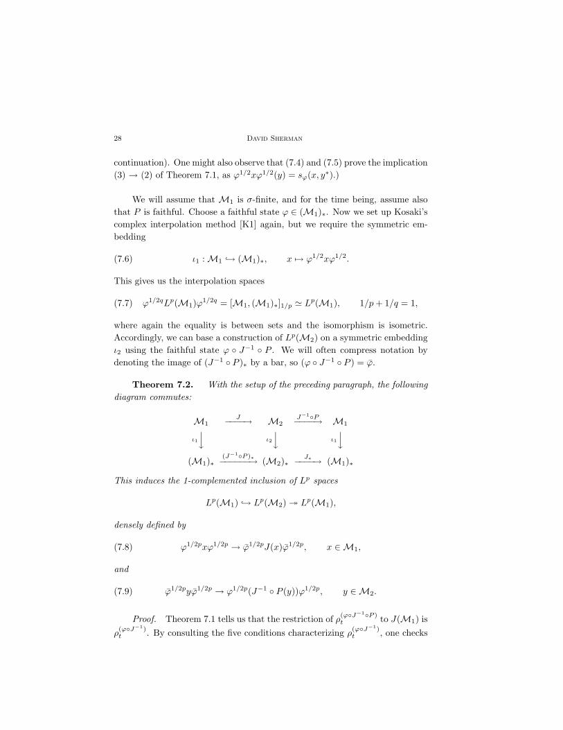
We will assume that M1 is σ-finite, and for the time being, assume alsothat P is faithful. Choose a faithful state ϕ ∈ (M1)∗. Now we set up Kosaki’scomplex interpolation method [K1] again, but we require the symmetric em-bedding
(7.6) ι1 : M1 ↪→ (M1)∗, x 7→ ϕ1/2xϕ1/2.
This gives us the interpolation spaces
(7.7) ϕ1/2qLp(M1)ϕ1/2q = [M1, (M1)∗]1/p ' Lp(M1), 1/p+ 1/q = 1,
where again the equality is between sets and the isomorphism is isometric.Accordingly, we can base a construction of Lp(M2) on a symmetric embeddingι2 using the faithful state ϕ ◦ J−1 ◦ P . We will often compress notation bydenoting the image of (J−1 ◦ P )∗ by a bar, so (ϕ ◦ J−1 ◦ P ) = ϕ.
Theorem 7.2. With the setup of the preceding paragraph, the followingdiagram commutes:
M1J−−−−→ M2
J−1◦P−−−−→ M1
ι1
y ι2
y ι1
y(M1)∗
(J−1◦P )∗−−−−−−→ (M2)∗J∗−−−−→ (M1)∗
This induces the 1-complemented inclusion of Lp spaces
Lp(M1) ↪→ Lp(M2) � Lp(M1),
densely defined by
(7.8) ϕ1/2pxϕ1/2p → ϕ1/2pJ(x)ϕ1/2p, x ∈M1,
and
(7.9) ϕ1/2pyϕ1/2p → ϕ1/2p(J−1 ◦ P (y))ϕ1/2p, y ∈M2.
Proof. Theorem 7.1 tells us that the restriction of ρ(ϕ◦J−1◦P )t to J(M1) is
ρ(ϕ◦J−1)t . By consulting the five conditions characterizing ρ(ϕ◦J−1)
t , one checks

Lp isometries 29
that it agrees with J ◦ ρϕt ◦J−1. (This “must” be true, as J is a normal Jordan*-isomorphism onto its image.) These facts imply
Φϕ(J(x)) =∫ρϕt (J(x))(coshπt)−1dt
=∫ρ(ϕ◦J−1)t (J(x))(coshπt)−1dt
=∫J ◦ ρϕt ◦ J−1(J(x))(coshπt)−1dt
= J
[∫ρϕt (x)(coshπt)−1dt
]= J(Φϕ(x)).
Now we are ready to check that the diagram in Theorem 7.2 commutes,starting with the left-hand square. This amounts to showing that for x ∈M1, y ∈M2,
(7.10) ϕ1/2J(x)ϕ1/2(y) = [(ϕ1/2xϕ1/2) ◦ J−1 ◦ P ](y).
We calculate
ϕ1/2J(x)ϕ1/2(y) = [ϕ • Φϕ(J(x))](y)
= ϕ(Φϕ(J(x)) • y)= ϕ((J(Φϕ(x))) • y)∗= ϕ(Φϕ(x) • (J−1 ◦ P (y)))
= ϕ1/2xϕ1/2(J−1 ◦ P (y))
= [(ϕ1/2xϕ1/2) ◦ J−1 ◦ P ](y).
We used Lemma 5.5(2) in the equality marked ∗=.For the right-hand square, we need to demonstrate that for x ∈ M1, y ∈
M2,[(ϕ1/2yϕ1/2) ◦ J ](x) = (ϕ1/2(J−1 ◦ P (y))ϕ1/2)(x).
But this equation is equivalent to (7.10), which was just shown.It again follows from general interpolation theory that the inclusion and
norm one projection extend to the interpolated spaces. Since ϕ1/2xϕ1/2 isidentified with ϕ1/2J(x)ϕ1/2, the equality (7.7) gives us (7.8) and (7.9).
Remark 7.3. Theorem 7.2 holds without change if P is not faithful.With q the support of P , replace M2 by qM2q, and notice that Lp(qM2q) 'qLp(M2)q ⊂ Lp(M2).

30 David Sherman
It also seems possible, if not pleasant, to extend Theorem 7.2 to non-σ-finite M1 by using a weight. When P is a normal conditional expectation,most of the necessary tools are in [Te2] and [I].
Remark 7.4. As mentioned, typicality may be related to a Jordan versionof (6.3) and (6.6). Cocycles are not symmetric objects (the “handedness” isapparent in the modular algebra realization (Dϕ : Dψ)t = ϕitψ−it), so onecannot expect either of these equations for the projection P . We can deriveat least something analogous using (7.10). Let faithful ϕ ≤ Cψ ∈ (M1)+∗ forsome C <∞, so y = (Dϕ : Dψ)−i/2(= ϕ1/2ψ−1/2) exists in M1. Now write
ϕ = ϕ ◦ J−1 ◦ P = ψ1/2y∗yψ1/2 ◦ J−1 ◦ P = ψ1/2J(y∗y)ψ1/2.
If we write z = (Dϕ : Dψ)−i/2, this gives z∗z = J(y∗y). Taking square roots,|z| = J(|y|), or
|(Dϕ : Dψ)−i/2| = J(|(Dϕ : Dψ)−i/2|).
§8. Factorization and typical isometries
We have not been able to show that the isometry constructed in (7.8) isgenerally independent of the choice of ϕ. We now introduce a hypothesis whichremoves the (possible) dependence.
Proposition 8.1. Let J : M1 →M2 be a normal Jordan *-monomorphismand P : M2 → J(M1) be a normal positive projection, with P factoring as
(8.1) P = P ′ ◦ F, F : M2 → J(M1)′′ a normal conditional expectation.
Then (1.1) (taking w = 1) defines an Lp isometry.If M1 is σ-finite, then this agrees with the Lp isometry (7.8) obtained in
Theorem 7.2 for any faithful normal state ϕ ∈ (M1)∗, and as a consequencethe range is 1-complemented.
Proof. It suffices to prove these statements for the map
(8.2) Lp(M1)+ 3 ϕ1/p 7→ (ϕ ◦ J−1 ◦ P ′)1/p ∈ Lp(J(M1)′′)+,
since precomposition with the conditional expectation F embeds Lp(J(M1)′′)in Lp(M2) as discussed in Section 6.
Now J is the sum of a *-homomorphism π and a *-antihomomorphismπ′, where π(1) and π′(1) are orthogonal and central in J(M1)′′. We may

Lp isometries 31
assume that the abelian summand of M1, if it exists, is in the support of πand not π′. This decomposes M1 into three summands: s(π)(1 − s(π′))M1,(1 − s(π))s(π′)M1, and s(π)s(π′)M1. Note that the images of the first twoare central summands of J(M1) which are multiplicatively closed, so theyare also central summands of J(M1)′′. Since P and P ′ respect this centraldecomposition (by Lemma 5.5), P ′ restricts to the identity on these, and weare in the situation of Proposition 6.3. It is left to discuss the third summand,so in the remainder of the proof we assume that s(π) = s(π′) = 1 and that M1
has no abelian summand.We first claim
J(M1)′′ = {π(x)⊕ π′(y) | x, y ∈M1} ' M1 ⊕Mop1 .
Let v ∈ M1 be a partial isometry with vv∗ = p ⊥ q = v∗v. Then J(M1)′′
contains(π(v)⊕ π′(v))(π(p)⊕ π′(p)) = 0⊕ π′(v)
and is closed under multiplication, addition, and adjoints, whence it is easy toverify the claim.
By Lemma 5.5(4), P ′(π(1) ⊕ 0) = J(λ) ∈ J(Z(M1)), where 0 ≤ λ ≤ 1.Then
P ′(π(x)⊕ 0) = P ′[(π(x)⊕ π′(x)) • (π(1)⊕ 0)](8.3)
= (π(x)⊕ π′(x)) • P ′(π(1)⊕ 0)
= π(x)π(λ)⊕ π′(x)π′(λ)
= J(xλ),
and similarly
P ′(0⊕ π′(y)) = π(y)π(1− λ)⊕ π′(y)π′(1− λ) = J(y(1− λ)).
Note that λ and 1 − λ must be nonsingular, because faithfulness of P ′ is aconsequence of s(P ) = P (1)(= J(1)). We obtain that
ϕ ◦ J−1 ◦ P ′ = (λϕ ◦ π−1)⊕ ((1− λ)ϕ ◦ π′−1).
The map (8.2) is then
ϕ1/p 7→ (λϕ ◦ π−1)1/p ⊕ ((1− λ)ϕ ◦ π′−1)1/p.
Since π and π′ induce (surjective) isometric isomorphisms at the Lp level ineach summand, this map has a linear extension to all of Lp(M1). The image of

32 David Sherman
ξ ∈ Lp(M1) is a vector whose two orthogonal components have norms ‖λ1/pξ‖and ‖(1− λ)1/pξ‖; it has total norm
(‖λ|ξ|p‖+ ‖(1− λ)|ξ|p‖)1/p = ‖|ξ|p‖1/p = ‖ξ‖.
Therefore the map is isometric.The second assertion of the proposition almost follows from the discus-
sion in Section 6 of Lp isometries induced by (possibly antimultiplicative) 1-complemented inclusions. There we noted that any left or right embeddinggave the same isometry, and so was typical. Here we make this statementexplicit for symmetric embeddings. So suppose ϕ1/2pxϕ1/2p = ψ1/2pyψ1/2p ∈Lp(M1)+. By taking square roots, we can find a partial isometry v ∈M1 withvx1/2ϕ1/2p = y1/2ψ1/2p. Considering first the antimultiplicative embedding,we know by (6.5) that
(ϕ ◦ π′−1)1/2pπ′(vx1/2) = (ψ ◦ π′−1)1/2pπ′(y1/2),
so
(ϕ ◦ π′−1)1/2pπ′(x)(ϕ ◦ π′−1)1/2p
= [(ϕ ◦ π′−1)1/2pπ′(vx1/2)][(ϕ ◦ π′−1)1/2pπ′(vx1/2)]∗
= [(ψ ◦ π′−1)1/2pπ′(y1/2)][(ψ ◦ π′−1)1/2pπ′(y1/2)]∗
= (ψ ◦ π′−1)1/2pπ′(y)(ψ ◦ π′−1)1/2p.
Obviously this relation extends off the positive cone. A similar calculationholds for π, so it holds for J . This means that the Lp isometry (7.8) does notdepend on the choice of state and therefore agrees with (8.2).
The papers [HS2], [St3] consider exactly the factorization (8.1) for projec-tions onto arbitrary JW-subalgebras, which includes our situation. They doconclude the factorization in case
1. Z(J(M1)) = Z(J(M1)′′); or
2. (M1, τ) is semifinite and the weight τ = τ ◦ J−1 ◦ P is semifinite.
In our situation, condition (1) precludes the presence of both multiplicative andantimultiplicative homomorphisms on a non-abelian summand, so J(M1) =J(M1)′′ and the conclusion is automatic. Our final result subsumes condition(2) by assuming only that M1 is AS.

Lp isometries 33
Proposition 8.2. Let J : M1 →M2 be a normal Jordan *-monomorphism,and P : M2 → J(M1) be a normal positive projection. If M1 is AS, then P
factors as P |J(M1)′′ ◦F , where F : M2 → J(M1)′′ is a normal conditionalexpectation.
Proof. First note that by the arguments in the beginning of the proof ofProposition 8.1, we may assume that J = π ⊕ π′, where M1 has no abeliansummand and both π, π′ are faithful.
We start with the case where (M1, τ) is finite, writing τ = τ ◦ J−1 ◦ P .In the proof of Theorem 5.6 we saw that J(M1)′′ is pointwise invariant underστ , so by Takesaki’s theorem [T1] there is a normal τ -preserving conditionalexpectation F : M2 → J(M1)′′. Now we use equations (7.2) and (7.3) tocalculate
sτ (P (F (y)), J(x)) = sτ (F (y), J(x)) = τ1/2J(x∗)τ1/2(F (y)) = τ(J(x∗)F (y))
= τ(J(x∗)y) = τ1/2J(x∗)τ1/2(y) = sτ (y, J(x)) = sτ (P (y), J(x))
for any x ∈ M1, y ∈ M2. This implies that P ◦ F = P , and the finite case iscomplete.
Now let {Mα, Eα} be a paving of M1 by finite subalgebras, and denoteby 1α the unit of Mα (which may not be the unit of M1). Write
Eα = J ◦ Eα ◦ J−1 : J(M1) → J(Mα).
Then Eα ◦ P is a positive normal projection onto the Jordan image of a finitealgebra, so by the first part of the proof we can factor it as
M2P−−−−→ J(M1)
Fα
y yEα
J(Mα)′′Sλα−−−−→ J(Mα)
Here Fα is a normal conditional expectation, and Sλαis the symmetrization
guaranteed by (8.3),
(8.4) Sλα: π(x)⊕ π′(y) 7→ J(λαx+ (1− λα)y),
where 0 ≤ λα ≤ 1α is an element of J(Z(Mα)). We also have, as before,that the nonsingular element J(λ) , P (π(1)) is in J(Z(M1)). The commutingsquare gives us the relation
Eα(J(λ)) = Eα ◦ P (π(1)) = Sλα◦ Fα(π(1)) = Sλα
(π(1α)) = J(λα).

34 David Sherman
This implies that λα = Eα(λ) s→ λ by Theorem 5.2(2).It remains to construct the conditional expectation. Since s(P ) = J(1)
by assumption, we only need to consider elements in J(1)M2J(1). We useJ(1) = π(1) + π′(1) to write a generic element as
y =(a bc d
),
where a ∈ π(1)M2π(1), etc. By Theorem 5.2(2) we have
(8.5) P (y) = s− lim Eα ◦ P (y) = s− limSλα ◦ Fα(y).
Since Fα is a conditional expectation and J(Mα) is inside the diagonal J(M1)′′,we may write
Fα(a bc d
)=
(F 1
α(a) 0
0 F 2α(d)
).
Then (8.5) becomes
(8.6) P (y) =
s− lim(π(λα)F 1
α(a)+π(1−λα)[π◦π′−1(F 2α(d))] 0
0 π′(λα)[π′◦π−1(F 1α(a))]+π′(1−λα)F 2
α(d)
),
which we claim can be written as
(8.7) P (y) = Sλ ◦ F (y), where F (y) = s− lim(F 1
α(a) 0
0 F 2α(d)
).
To establish the claim, we check that (i) the strong limits in the definitionof F do exist, (ii) the factorization (8.7) is correct, (iii) F is normal, (iv) Fis contractive, (v) the range of F is contained in J(M1)′′, and (vi) F fixesJ(M1)′′.
We have from the above that
P (( a 00 0 )) = s− lim
(π(λα)F 1
α(a) 0
0 π′(λα)[π′◦π−1(F 1α(a))]
),
so π(λα)F 1α(a) is strongly convergent. We now represent π(M) faithfully
and nondegenerately as an algebra of operators on a Hilbert space, and leten = e[1/n, 1] be spectral projections of π(λ). Since λ is nonsingular, theseprojections increase to π(1). Given any vector ξ, we have
‖[F 1α(a)− F 1
β (a)]ξ‖ ∼ ‖[F 1α(a)− F 1
β (a)]enξ‖= ‖[F 1
α(a)− F 1β (a)]π(λ)(π(λ)−1enξ)‖
= ‖((F 1α(a)[π(λ)− π(λα)] + [π(λα)F 1
α(a)− π(λβ)F 1β (a)]
+ F 1β (a)[π(λ)− π(λβ)])(π(λ)−1enξ)‖
→ 0 as α, β increase.

Lp isometries 35
Note that the first approximation can be made independent of α and β since{F 1
α(a)} is a norm-bounded set. The same argument establishes the strong con-vergence of F 2
α(d), and (i) is obtained. Since π(λα), F 1α(a), F 2
α(d) are stronglyconvergent, (ii) follows from (8.6).
For (iii), again it suffices by symmetry to check that
(8.8) π(1)M2π(1) 3 xγs→ x⇒ F
((xγ 00 0
)) s→ F (( x 00 0 )) .
(All limits in this paragraph are along increasing γ.) Since P is normal, wehave
P((
xγ 00 0
)) s→ P (( x 00 0 ))
and thenSλ
((s−limα F
1α(xγ) 0
0 0
))s→ Sλ
((s−limα F
1α(x) 0
0 0
)).
Reading off the upper left entry,
π(λ)[s− limαF 1α(xγ)]
s→ π(λ)[s− limαF 1α(x)].
By an approximation argument similar to that of the previous paragraph,
s− limαF 1α(xγ)
s→ s− limαF 1α(x).
But this is exactly the conclusion of (8.8), and we have (iii).Now (iv) and (v) are automatic from the form of F , and (vi) follows from
the normality of F and the fact that F fixes ∪J(Mα)′′. The proof is complete.
The preceding propositions may seem somewhat technical, but they canbe summarized nicely.
Theorem 8.3. Let J : M1 →M2 be a normal Jordan *-monomorphism,and let P : M2 → J(M1) be a normal positive projection. Each condition belowimplies its successor:
1. M1 is AS;
2. the projection P factors through a conditional expectation onto J(M1)′′;
3. the map ϕ1/p 7→ (ϕ ◦ J−1 ◦ P )1/p, ϕ ∈ (M1)+∗ , extends linearly to anisometry from Lp(M1) to Lp(M2).
§9. Conclusion

36 David Sherman
From Theorems 1.2 and 8.3, we have arrived at a complete description ofall the isometries from Lp(M1) to Lp(M2), provided that M1 is AS. They aretypical, arising via (1.1), and arbitrary data J, P,w are allowed. When M1 isonly assumed to have EPp and EP1, which may be weaker, we can still saythat all Lp isometries are typical.
The main motivation for this paper was to develop Watanabe’s ideas, es-pecially EP, as far as possible. This certainly provides new methods and in-formation, but we have only been able to apply them to Questions 1.1 and 1.3when the initial algebra is well-approximated by semifinite algebras. We donot claim that further work in this direction is necessary for a solution to oneor both of these questions. It certainly seems possible that another techniquemay produce a relatively straightforward solution - for example, the paper [S1]handles the surjective case by different methods. Nonetheless, we do think thatEPp, AS, and condition (2) from Theorem 8.3 are worth investigating on theirown merits, and our work here shows their relation to Lp isometries.
References
[B] Banach, S., Theorie des operations lineaires, Warsaw, 1932.[BW1] Bunce, L. J., and Wright, J. D. Maitland, On orthomorphisms between von Neu-
mann preduals and a problem of Araki, Pacific J. Math., 158 (1993), no. 2, 265-272.[BW2] Bunce, L. J., and Wright, J. D. Maitland, The Mackey-Gleason problem for vector
measures on projections in von Neumann algebras, J. London Math. Soc. (2), 49(1994), no. 1, 133-149.
[Ch] Christensen, E., Measures on projections and physical states, Comm. Math. Phys.,86 (1982), no. 4, 529-538.
[C1] Connes, A., Une classification des facteurs de type III, Ann. Sci. Ecole Norm. Sup.,6 (1973), 133-252.
[C2] Connes, A., Almost periodic states and factors of type III1, J. Funct. Anal., 16(1974), 415-445.
[C3] Connes, A., Classification of injective factors. Cases II1, II∞, IIIλ, λ 6= 1, Ann.Math. (2), 104 (1976), no. 1, 73-115.
[C4] Connes, A., Noncommutative geometry, Harcourt Brace & Co., San Diego, 1994.[D] Dye, H., On the geometry of projections in certain operator algebras, Ann. Math.,
61 (1955), 73-88.[DR] Dye, H., and Russo, B., A note on unitary operators in C*-algebras, Duke Math.
J., 33 (1966), 413-416.[ES] Effros, E., and Størmer, E., Positive projections and Jordan structure in operator
algebras, Math. Scand., 45 (1979), no. 1, 127-138.[FT] Falcone, T., and Takesaki, M., The non-commutative flow of weights on a von
Neumann algebra, J. Funct. Anal., 182 (2001), no. 1, 170-206.[FJ] Fleming, R., and Jamison, J., Isometries on Banach spaces: function spaces, Chap-
man & Hall/CRC, Boca Raton, 2003.[G] Gleason, A., Measures on the closed subspaces of a Hilbert space, J. Math. Mech.,
6 (1957), 885-893.

Lp isometries 37
[GGMS] Ghoussoub, N., Godefroy, G., Maurey, B., and Schachermayer, W., Some topo-logical and geometrical structures in Banach spaces, Mem. Amer. Math. Soc., 70(1987), no. 378.
[H1] Haagerup, U., Lp-spaces associated with an arbitrary von Neumann algebra,Algebres d’operateurs et leurs applications en physique mathematique, CNRS 15(1979), 175-184.
[H2] Haagerup, U., Connes’ bicentralizer problem and uniqueness of the injective factorof type III1, Acta Math., 158 (1987), 95-148.
[HH] Haagerup, U., and Hanche-Olsen, H., Tomita-Takesaki theory for Jordan algebras,J. Operator Theory, 11 (1984), 343-364.
[HRS] Haagerup, U., Rosenthal, H., and Sukochev, F., Banach embedding properties ofnon-commutative Lp-spaces, Mem. Amer. Math. Soc., 163 (2003), no. 776.
[HS1] Haagerup, U., and Størmer, E., Equivalence of normal states on von Neumannalgebras and the flow of weights, Adv. Math., 83 (1990), 180-262.
[HS2] Haagerup, U., and Størmer, E., Positive projections of von Neumann algebras ontoJW-algebras, Rep. Math. Phys., 36 (1995), no. 2-3, 317-330.
[HvN] Halmos, P., and von Neumann, J., Operator methods in classical mechanics II,Ann. of Math., 43 (1942), 332-350.
[He] Herman, R., Centralizers and an ordering for faithful, normal states, J. Funct.Anal., 13 (1973), 317-323.
[HT] Herman, R., and Takesaki, M., States and automorphism groups of operator alge-bras, Comm. Math. Phys., 19 (1970), 142-160.
[I] Izumi, H., Constructions of non-commutative Lp-spaces with a complex parameterarising from modular actions, Internat. J. Math., 8 (1997), no. 8, 1029-1066.
[J] Junge, M., Doob’s inequality for non-commutative martingales, J. Reine Angew.Math., 549 (2002), 149-190.
[JRS] Junge, M., Ruan, Z.-J., and Sherman, D., A classification for 2-isometries of non-commutative Lp-spaces, Israel J. Math., to appear.
[JRX] Junge, M., Ruan, Z.-J., and Xu, Q., Rigid OLp structures of non-commutative Lp-spaces associated with hyperfinite von Neumann algebras, Math. Scand., to appear.
[JS] Junge, M., and Sherman, D., Noncommutative Lp modules, J. Operator Theory,to appear.
[JX] Junge, M., and Xu, Q., Noncommutative Burkholder/Rosenthal inequalities, Ann.Probab., 31 (2003), no. 2, 948-995.
[Ka] Kadison, R. V., Isometries of operator algebras, Ann. Math., 54 (1951), 325-338.[Ki] Kirchberg, E., On nonsemisplit extensions, tensor products and exactness of group
C*-algebras, Invent. Math., 112 (1993), no. 3, 449-489.[K1] Kosaki, H., Applications of the complex interpolation method to a von Neumann
algebra: non-commutative Lp spaces, J. Funct. Anal., 56 (1984), 29-78.[K2] Kosaki, H., Applications of uniform convexity of noncommutative Lp-spaces, Trans.
Amer. Math. Soc., 283 (1984), no. 1, 265-282.[L] Lamperti, J., On the isometries of certain function spaces, Pacific J. Math., 8
(1958), 459-466.[N] Nelson, E., Notes on non-commutative integration, J. Funct. Anal., 15 (1974),
103-116.[PX] Pisier, G., and Xu, Q., Noncommutative Lp spaces, in: Johnson, W. B., and Lin-
denstrauss, J., eds., Handbook of the geometry of Banach spaces, Vol. II (North-Holland Publishing Co., Amsterdam, 2003), 1459-1517.
[R] Raynaud, Y., On ultrapowers of non commutative Lp spaces, J. Operator Theory,48 (2002), 41-68.
[RX] Raynaud, Y., and Xu, Q., On subspaces of non-commutative Lp-spaces, J. Funct.Anal., 203 (2003), 149-196.
[Sc] Schmitt, L., The Radon-Nikodym theorem for Lp-spaces of W ∗-algebras, Publ. Res.Inst. Math. Sci., 22 (1986), 1025-1034.

38 David Sherman
[Se] Segal, I., A non-commutative extension of abstract integration, Ann. of Math., 57(1953), 401-457.
[S1] Sherman, D., Noncommutative Lp structure encodes exactly Jordan structure, J.Funct. Anal., to appear.
[S2] Sherman, D., Applications of modular algebras, in preparation.[St1] Størmer, E., On the Jordan structure of C*-algebras, Trans. Amer. Math. Soc.,
120 (1965), 438-447.[St2] Størmer, E., Decomposition of positive projections on C*-algebras, Math. Ann.,
247 (1980), no. 1, 21-41.[St3] Størmer, E., Conditional expectations and projection maps of von Neumann alge-
bras, Operator algebras and applications (Kluwer Acad. Publ., Dordrecht, 1997),449-461.
[T1] Takesaki, M., Conditional expectations in von Neumann algebras, J. Funct. Anal.,9 (1972), 306-321.
[T2] Takesaki, M., Theory of operator algebras II, Springer-Verlag, New York, 2002.[Te1] Terp, M., Lp-spaces associated with von Neumann algebras, notes, Copenhagen
University, 1981.[Te2] Terp, M., Interpolation spaces between a von Neumann algebra and its predual, J.
Operator Theory, 8 (1982), no. 2, 327-360.[Ts] Tsukada, M., Strong convergence of martingales in von Neumann algebras, Proc.
Amer. Math. Soc., 88 (1983), 537-540.[vD] van Daele, A., A new approach to the Tomita-Takesaki theory of generalized Hilbert
algebras, J. Funct. Anal., 15 (1974), 378-393.[W1] Watanabe, K., An application of orthoisomorphisms to non-commutative Lp-
isometries, Publ. Res. Inst. Math. Sci., 32 (1996), 493-502.[W2] Watanabe, K., Problems on isometries of non-commutative Lp-spaces, Function
spaces (Edwardsville, IL, 1998), 349-356, Contemp. Math., 232, Amer. Math. Soc.,Providence, RI, 1999.
[W3] Watanabe, K., On the structure of non-commutative Lp isometries, preprint.[Wo] Woronowicz, S., Selfpolar forms and their applications to the C*-algebra theory,
Rep. Math. Phys., 6 (1974), no. 3, 487-495.[Ya] Yamagami, S., Algebraic aspects in modular theory, Publ. Res. Inst. Math. Sci.,
28 (1992), 1075-1106.[Y1] Yeadon, F. J., Isometries of non-commutative Lp spaces, Math. Proc. Camb. Phil.
Soc., 90 (1981), 41-50.[Y2] Yeadon, F. J., Measures on projections in W*-algebras of type II1, Bull. London
Math. Soc., 15 (1983), no. 2, 139-145.