on the use of the micro-macro decomposition to design
TRANSCRIPT

On the use of the micro-macro decomposition to design
multiscale numerical schemes for kinetic equations
Luc Mieussens
Institut de Mathematiques de Bordeaux,Universite de Bordeaux,
France
Workshop “Computational Kinetic Transport and Hybrid Methods”,2009 (IPAM, UCLA)
collaborators: P. Degond (Toulouse), G. Dimarco (Ferrara), M. Lemou (Rennes), J.-G. Liu
(Duke)
Luc Mieussens (Bordeaux) multiscale numerical schemes KTWS1 1 / 37

Kinetic equations and asymptotic models
scale factor: ε = mean free pathmacroscopic length (Knudsen number)
when ε ≪ 1: the kinetic equation is well approximated by anasymptotic ”fluid” model
Example 1: Rarefied gas dynamics (hydrodynamic limit)
∂t f + v · ∇f =1
εQ(f )
↓ ε ≪ 1
∂tU + ∇ · F (U) + ε∇ · (D∇U) = 0
(compressible Navier-Stokes eq. for U =∫(1, v , 1
2 |v |2)f dv)
↓ ε = 0
∂tU + ∇ · F (U) = 0
(compressible Euler eq.)other limits: low Mach number, boundary driven diffusion, ...
Luc Mieussens (Bordeaux) multiscale numerical schemes KTWS1 2 / 37

Kinetic equations and asymptotic models
scale factor: ε = mean free pathmacroscopic length (Knudsen number)
when ε ≪ 1: the kinetic equation is well approximated by anasymptotic ”fluid” model
Example 2: Linear transport (diffusion limit)
∂t f +1
εv · ∇f =
1
ε2L(f )
↓ ε = 0
∂tρ −∇ ·(κ∇ρ
)= 0
diffusion eq for ρ = 〈f 〉
Luc Mieussens (Bordeaux) multiscale numerical schemes KTWS1 2 / 37

Multiscale kinetic problems
multiscale: ε = O(1) in some zones, ε ≪ 1 in others
Kinetic
shoc
kFluid
������������������������������������������������������������������������������������������������������������������������������������������������������������������������������������������������������������������������������������������������������������������������������������������������������������������������������������������������������������������������������������������
������������������������������������������������������������������������������������������������������������������������������������������������������������������������������������������������������������������������������������������������������������������������������������������������������������������������������������������������������������������������������������������
diffusionkinetic
aerodynamics (Boltzmann) linear transport
usual numerical schemes: numerical constraint ∆t and ∆x = O(ε)cannot be used when ε ≪ 1
solutions:1 domain decomposition2 extended fluid models (higher order, moments, ...)3 AP schemes
this talk: a general method for (1), (2), (3)
Luc Mieussens (Bordeaux) multiscale numerical schemes KTWS1 3 / 37
Outline
1 AP schemesDefinitionCounter-exampleReferences
2 AP scheme for the (linear) diffusion limitMicro-macro decompositionDiscretizationNumerical tests
3 AP scheme for the compressible asymptotics of the Boltzmann equationThe Boltzmann equationAP scheme based on the micro-macro decompositionNumerical test
4 Fluid models with localized kinetic upscalingLocalization of the deviation partNumerical tests
Luc Mieussens (Bordeaux) multiscale numerical schemes KTWS1 4 / 37

Outline
1 AP schemesDefinitionCounter-exampleReferences
2 AP scheme for the (linear) diffusion limitMicro-macro decompositionDiscretizationNumerical tests
3 AP scheme for the compressible asymptotics of the Boltzmann equationThe Boltzmann equationAP scheme based on the micro-macro decompositionNumerical test
4 Fluid models with localized kinetic upscalingLocalization of the deviation partNumerical tests
Luc Mieussens (Bordeaux) multiscale numerical schemes KTWS1 5 / 37

Asymptotic Preserving (AP) schemes.
definition: a scheme uniformly stable and accurate w.r.t ε (∆t and∆x independent of ε)
consequence: in the fluid regime (ε ≪ 1): scheme consistent with thefluid equation
requirements: special time (implicit) and space discretizations
Luc Mieussens (Bordeaux) multiscale numerical schemes KTWS1 6 / 37
Asymptotic Preserving (AP) schemes
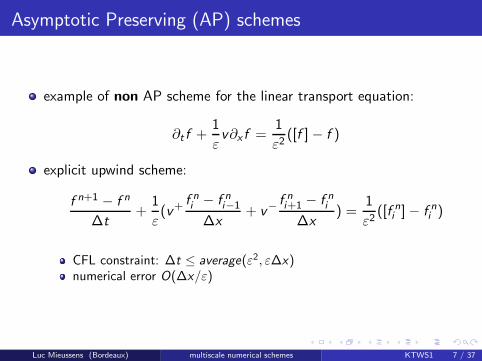
example of non AP scheme for the linear transport equation:
∂t f +1
εv∂x f =
1
ε2([f ] − f )
explicit upwind scheme:
f n+1 − f n
∆t+
1
ε(v+ f n
i − f ni−1
∆x+ v−
f ni+1 − f n
i
∆x) =
1
ε2([f n
i ] − f ni )
CFL constraint: ∆t ≤ average(ε2, ε∆x)numerical error O(∆x/ε)
Luc Mieussens (Bordeaux) multiscale numerical schemes KTWS1 7 / 37

Linear transport: contributions of Larsen, Morel, Miller,
Adams, . . .
linear transport equation (neutron transport) and its diffusion limit
fully implicit scheme (collision and transport)
main problem: AP space discretization for the steady equation
study of different space discretizations
main result: Discontinuous Galerkin (P1) approximation is AP
Luc Mieussens (Bordeaux) multiscale numerical schemes KTWS1 8 / 37

Unsteady equations: contributions of Klar, Jin, . . .
main ingredients:
time splitting scheme, semi-implicit (collision)decomposition of the solution (even-odd decomposition, zero-first orderdecomposition)
contribution of A. Klar: linear transport and its diffusion limit,Boltzmann equation and the low Mach number limit
contribution of S. Jin (with Pareschi, Toscani, Russo, Caflisch): lineartransport, and some hyperbolic systems with relaxation (toy modelsfor kinetic equations)
other works: Goudon-Lafitte, Gosse-Toscani, ...
Luc Mieussens (Bordeaux) multiscale numerical schemes KTWS1 9 / 37
Our contribution
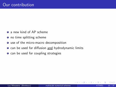
a new kind of AP scheme
no time splitting scheme
use of the micro-macro decomposition
can be used for diffusion and hydrodynamic limits
can be used for coupling strategies
Luc Mieussens (Bordeaux) multiscale numerical schemes KTWS1 10 / 37
Outline
1 AP schemesDefinitionCounter-exampleReferences
2 AP scheme for the (linear) diffusion limitMicro-macro decompositionDiscretizationNumerical tests
3 AP scheme for the compressible asymptotics of the Boltzmann equationThe Boltzmann equationAP scheme based on the micro-macro decompositionNumerical test
4 Fluid models with localized kinetic upscalingLocalization of the deviation partNumerical tests
Luc Mieussens (Bordeaux) multiscale numerical schemes KTWS1 11 / 37

Diffusion limit of the linear transport equation[M.Lemou-LM, SISC 2008]
linear transport equation:
∂t f +1
εv∂x f =
1
ε2([f ] − f )
where [f ] =1
2
∫ 1
−1f (v) dv
limit ε = 0: diffusion equation for ρ = [f ]
∂tρ − ∂x(κ∂xρ) = 0
collision and transport are stiff
Luc Mieussens (Bordeaux) multiscale numerical schemes KTWS1 12 / 37

Micro-macro decomposition.
kinetic equation:
∂t f +1
εv∂x f =
1
ε2([f ] − f )
micro-macro decomposition: f = ρ + εg , where ρ = [f ]property: [g ] = 0
decomposition of the kinetic equation:
∂tρ + ε∂tg +1
εv∂xρ + v∂xg = −
1
εg
scale separation: evolution equations for ρ and g
∂tρ + ∂x [vg ] = 0,
∂tg +1
εv∂xg = −
1
ε2g − (
1
ε∂tρ +
1
ε2v∂xρ)
Luc Mieussens (Bordeaux) multiscale numerical schemes KTWS1 13 / 37

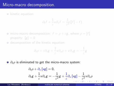
Micro-macro decomposition.
kinetic equation:
∂t f +1
εv∂x f =
1
ε2([f ] − f )
micro-macro decomposition: f = ρ + εg , where ρ = [f ]property: [g ] = 0
decomposition of the kinetic equation:
∂tρ + ε∂tg +1
εv∂xρ + v∂xg = −
1
εg
∂tρ is eliminated to get the micro-macro system:
∂tρ + ∂x [vg ] = 0,
∂tg +1
εv∂xg = −
1
ε2g − (
1
ε∂tρ +
1
ε2v∂xρ)
Luc Mieussens (Bordeaux) multiscale numerical schemes KTWS1 13 / 37
Micro-macro decomposition.
kinetic equation:
∂t f +1
εv∂x f =
1
ε2([f ] − f )
micro-macro decomposition: f = ρ + εg , where ρ = [f ]property: [g ] = 0
decomposition of the kinetic equation:
∂tρ + ε∂tg +1
εv∂xρ + v∂xg = −
1
εg
∂tρ is eliminated to get the micro-macro system:
∂tρ + ∂x [vg ] = 0,
∂tg +1
εv∂xg = −
1
ε2g +
1
ε∂x [vg ] −
1
ε2v∂xρ
Luc Mieussens (Bordeaux) multiscale numerical schemes KTWS1 13 / 37

Micro-macro decomposition.
kinetic equation:
∂t f +1
εv∂x f =
1
ε2([f ] − f )
micro-macro decomposition: f = ρ + εg , where ρ = [f ]property: [g ] = 0
decomposition of the kinetic equation:
∂tρ + ε∂tg +1
εv∂xρ + v∂xg = −
1
εg
∂tρ is eliminated to get the micro-macro system:
∂tρ + ∂x [vg ] = 0,
∂tg +1
ε(I − [.])(v∂xg) = −
1
ε2g −
1
ε2v∂xρ
(equivalent to the original equation (no approximation))
Luc Mieussens (Bordeaux) multiscale numerical schemes KTWS1 13 / 37
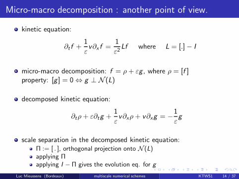
Micro-macro decomposition : another point of view.
kinetic equation:
∂t f +1
εv∂x f =
1
ε2Lf where L = [.] − I
micro-macro decomposition: f = ρ + εg , where ρ = [f ]property: [g ] = 0 ⇔ g ⊥ N (L)
decomposed kinetic equation:
∂tρ + ε∂tg +1
εv∂xρ + v∂xg = −
1
εg
scale separation in the decomposed kinetic equation:Π := [ . ], orthogonal projection onto N (L)applying Πapplying I − Π gives the evolution eq. for g
Luc Mieussens (Bordeaux) multiscale numerical schemes KTWS1 14 / 37
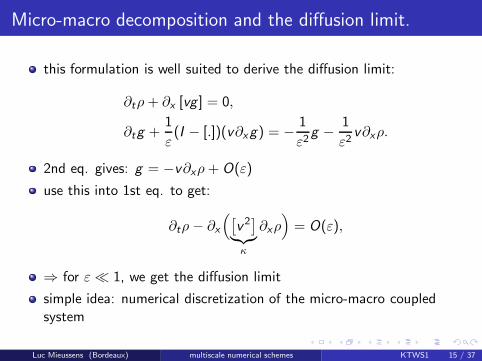
Micro-macro decomposition and the diffusion limit.
this formulation is well suited to derive the diffusion limit:
∂tρ + ∂x [vg ] = 0,
∂tg +1
ε(I − [.])(v∂xg) = −
1
ε2g −
1
ε2v∂xρ.
2nd eq. gives: g = −v∂xρ + O(ε)
use this into 1st eq. to get:
∂tρ − ∂x
([v2]
︸︷︷︸
κ
∂xρ)
= O(ε),
⇒ for ε ≪ 1, we get the diffusion limit
simple idea: numerical discretization of the micro-macro coupledsystem
Luc Mieussens (Bordeaux) multiscale numerical schemes KTWS1 15 / 37
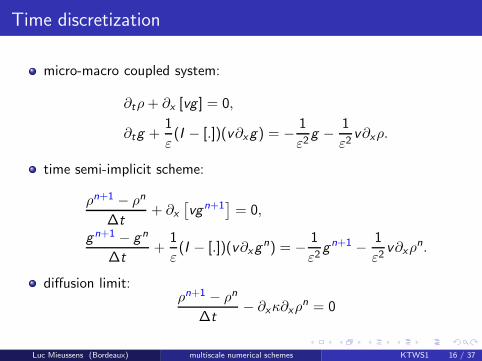
Time discretization
micro-macro coupled system:
∂tρ + ∂x [vg ] = 0,
∂tg +1
ε(I − [.])(v∂xg) = −
1
ε2g −
1
ε2v∂xρ.
time semi-implicit scheme:
ρn+1 − ρn
∆t+ ∂x
[vgn+1
]= 0,
gn+1 − gn
∆t+
1
ε(I − [.])(v∂xgn) = −
1
ε2gn+1 −
1
ε2v∂xρ
n.
diffusion limit:ρn+1 − ρn
∆t− ∂xκ∂xρ
n = 0
Luc Mieussens (Bordeaux) multiscale numerical schemes KTWS1 16 / 37
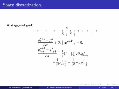
Space discretization.
staggered grid:ρi
gi− 1
2gi+ 1
2
ρn+1i − ρn
i
∆t+ ∂x
[vgn+1
]
i= 0,
gn+1i+ 1
2
− gni+ 1
2
∆t+
1
ε(I − [.])v∂xg
ni+ 1
2
= −1
ε2gn+1i+ 1
2
−1
ε2v∂xρ
ni+ 1
2.
Luc Mieussens (Bordeaux) multiscale numerical schemes KTWS1 17 / 37

Space discretization.
staggered grid:ρi
gi− 1
2gi+ 1
2
ρn+1i − ρn
i
∆t+ ∂x
[vgn+1
]
i= 0,
gn+1i+ 1
2
− gni+ 1
2
∆t+
1
ε(I − [.])v∂xg
ni+ 1
2
= −1
ε2gn+1i+ 1
2
−1
ε2v∂xρ
ni+ 1
2
.
upwind discretization of v∂xgi+ 12
(stability for kinetic regime)
Luc Mieussens (Bordeaux) multiscale numerical schemes KTWS1 17 / 37
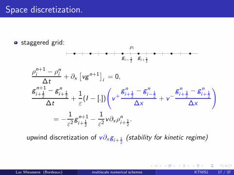
Space discretization.
staggered grid:ρi
gi− 1
2gi+ 1
2
ρn+1i − ρn
i
∆t+ ∂x
[vgn+1
]
i= 0,
gn+1i+ 1
2
− gni+ 1
2
∆t+
1
ε(I − [.])
(
v+gni+ 1
2
− gni− 1
2
∆x+ v−
gni+ 3
2
− gni+ 1
2
∆x
)
= −1
ε2gn+1i+ 1
2
−1
ε2v∂xρ
ni+ 1
2
.
central discretization of ∂x [vg ]i and v∂xρi+ 12
(for accurate approx. of the diffusion terms)
Luc Mieussens (Bordeaux) multiscale numerical schemes KTWS1 17 / 37

Space discretization.
staggered grid:ρi
gi− 1
2gi+ 1
2
ρn+1i − ρn
i
∆t+
vgn+1i+ 1
2
− gn+1i− 1
2
∆x
= 0,
gn+1i+ 1
2
− gni+ 1
2
∆t+
1
ε(I − [.])
(
v+gni+ 1
2
− gni− 1
2
∆x+ v−
gni+ 3
2
− gni+ 1
2
∆x
)
= −1
ε2gn+1i+ 1
2
−1
ε2v
ρni+1 − ρn
i
∆x.
central discretization of ∂x [vg ]i and v∂xρi+ 12
(for accurate approx. of the diffusion terms)
Luc Mieussens (Bordeaux) multiscale numerical schemes KTWS1 17 / 37
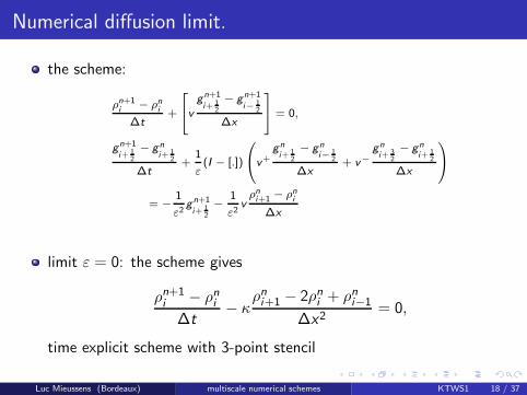
Numerical diffusion limit.
the scheme:
ρn+1i
− ρni
∆t+
2
4v
gn+1
i+ 12
− gn+1
i− 12
∆x
3
5 = 0,
gn+1
i+ 12
− gn
i+ 12
∆t+
1
ε(I − [.])
0
@v+gn
i+ 12
− gn
i− 12
∆x+ v−
gn
i+ 32
− gn
i+ 12
∆x
1
A
= −
1
ε2gn+1
i+ 12
−
1
ε2v
ρni+1 − ρn
i
∆x
limit ε = 0: the scheme gives
ρn+1i − ρn
i
∆t− κ
ρni+1 − 2ρn
i + ρni−1
∆x2= 0,
time explicit scheme with 3-point stencil
Luc Mieussens (Bordeaux) multiscale numerical schemes KTWS1 18 / 37

Analysis[J.-G Liu-LM, 2009]
the scheme is uniformly stable:
‖ρn‖2 + ε2|||gn|||2 ≤ C(‖ρ0‖2 + ε2|||g0|||2
)
under the CFL constraint:
∆t ≤1
2(∆x2
4κ+ ε∆x)
small ε: ∆t ≤ ∆x2
8κ (CFL for diffusion)
large ε: ∆t ≤ 12ε∆x (CFL for convection)
the scheme is uniformly accurate:
‖ρ(tn) − ρn‖ + ε|||g(tn) − gn||| ≤ C (∆t + ∆x2 + ε∆x)
Luc Mieussens (Bordeaux) multiscale numerical schemes KTWS1 19 / 37

Numerical tests
0 0.2 0.4 0.6 0.8 10
0.1
0.2
0.3
0.4
0.5
0.6
0.7
0.8
explicitLM 25LM 200
ε = 1
0 0.2 0.4 0.6 0.8 10
0.1
0.2
0.3
0.4
0.5
0.6
0.7
0.8
0.9
1
diffusionLM 25LM 200
ε = 10−8
0 0.1 0.2 0.3 0.4 0.50.2
0.3
0.4
0.5
0.6
0.7
explicitdiffusionLM 25LM 200JPT 25JPT 200K 25K 200
ε = 10−2
0 0.05 0.1 0.15 0.2 0.25 0.3 0.35 0.4 0.45 0.50.2
0.3
0.4
0.5
0.6
0.7
diffusionLM 25LM 200JPT 25JPT 200K 25K 200
ε = 10−4
Luc Mieussens (Bordeaux) multiscale numerical schemes KTWS1 20 / 37
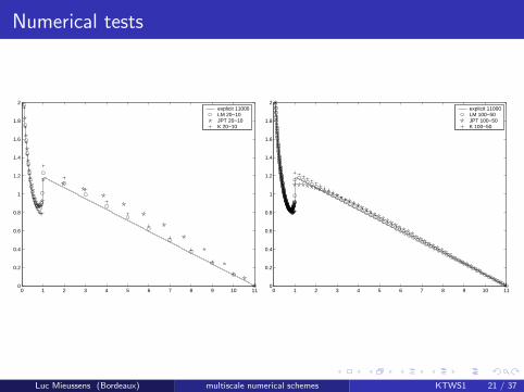
Numerical tests
0 1 2 3 4 5 6 7 8 9 10 110
0.2
0.4
0.6
0.8
1
1.2
1.4
1.6
1.8
2explicit 11000LM 20−10JPT 20−10K 20−10
0 1 2 3 4 5 6 7 8 9 10 110
0.2
0.4
0.6
0.8
1
1.2
1.4
1.6
1.8
2explicit 11000LM 100−50JPT 100−50K 100−50
Luc Mieussens (Bordeaux) multiscale numerical schemes KTWS1 21 / 37

Outline
1 AP schemesDefinitionCounter-exampleReferences
2 AP scheme for the (linear) diffusion limitMicro-macro decompositionDiscretizationNumerical tests
3 AP scheme for the compressible asymptotics of the Boltzmann equationThe Boltzmann equationAP scheme based on the micro-macro decompositionNumerical test
4 Fluid models with localized kinetic upscalingLocalization of the deviation partNumerical tests
Luc Mieussens (Bordeaux) multiscale numerical schemes KTWS1 22 / 37

The Boltzmann equation and its compressible limits.
Boltzmann equation:
∂t f + v · ∇x f =1
εQ(f , f )
ε = 0: f = M(U) ⇒ Euler equations:
∂tU + ∇x · F (U) = 0
where U = (ρ, ρu,E ) = 〈mf 〉, m = (1, v , 12 |v |
2)
ε ≪ 1: f = M(U) + O(ε) ⇒ compressible Navier-Stokes equations(CNS) :
∂tU + ∇x · F (U) = −ε
0∇x · σ
∇x · (σu + q)
Luc Mieussens (Bordeaux) multiscale numerical schemes KTWS1 23 / 37

A simple non-AP scheme.
Example: time splitting scheme of Coron-Perthame for the BGK equation
transport step: fn+ 1
2 −f n
∆t+ v · ∇x f
n = 0
relaxation step: f n+1 = e−∆t/εf n+ 12 + (1 − e−∆t/ε)M(f n+1)
(exact solution of: ∂t f = 1ε(M(f ) − f )
Property: scheme consistent with Euler equations, but not with CNSequations:
f n+1 − M(f n+1) = O(e−∆t/ε) ≪ O(ε)
Luc Mieussens (Bordeaux) multiscale numerical schemes KTWS1 24 / 37

AP scheme based on the micro-macro decomposition.[Bennoune-Lemou-LM, JCP 08]
micro-macro decomposition: f = M[U] + εgproperty: 〈mf 〉 = 〈mM[U]〉 = U and 〈mg〉 = 0
collision operator:
Q(f , f ) = Q(M(U),M(U)) + ε2Q(M(U), g) + ε2Q(g , g)
= 0 + εLM(U)g + ε2Q(g , g)
Boltzmann equation
∂tM(U) + v · ∇xM(U) + ε(∂tg + v · ∇xg) = LM(U)g + εQ(g , g)
property: g ⊥ N (LM(U))
define ΠM(U): orthogonal projection onto N (LM(U))
scale separation: apply ΠM(U) and I − ΠM(U)
Luc Mieussens (Bordeaux) multiscale numerical schemes KTWS1 25 / 37

AP scheme based on the micro-macro decomposition.
coupled system:
∂tU + ∇x · F (U) + ε∇x · 〈vmg〉 = 0,
∂tg + (I − ΠM(U))(v · ∇xg) =1
εLM(U)g + Q(g , g)
−1
ε(I − ΠM(U))(v · ∇xM(U)).
equivalent to the Boltzmann equation (no approximation!)
can be viewed as a fluid model (Euler) plus an upscaling term whichtakes kinetic effects into account
Luc Mieussens (Bordeaux) multiscale numerical schemes KTWS1 26 / 37
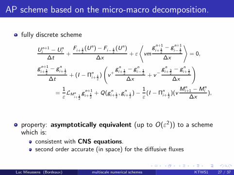
AP scheme based on the micro-macro decomposition.
fully discrete scheme
Un+1i − Un
i
∆t+
Fi+ 12(Un) − Fi− 1
2(Un)
∆x+ ε
*
vmgn+1
i+ 12
− gn+1
i− 12
∆x
+
= 0,
gn+1
i+ 12
− gn
i+ 12
∆t+ (I − Πn
i+ 12)
v+
gn
i+ 12− gn
i− 12
∆x+ v
−
gn
i+ 32− gn
i+ 12
∆x
!
=1
εLMn
i+ 12
gn+1
i+ 12
+ Q(gn
i+ 12, g
n
i+ 12) −
1
ε(I − Πn
i+ 12)(v
Mni+1 − Mn
i
∆x),
property: asymptotically equivalent (up to O(ε2)) to a schemewhich is:
consistent with CNS equations.second order accurate (in space) for the diffusive fluxes
Luc Mieussens (Bordeaux) multiscale numerical schemes KTWS1 27 / 37

Numerical test.
0 0,2 0,4 0,6 0,8 1x
-5
-2,5
0
2,5
5
7,5
10
q
APSiSeNS
0 0,2 0,4 0,6 0,8 1x
-7,5
-5
-2,5
0
2,5
5
7,5
10
q
Sod test case: heat flux (scaled)(ε = 2 × 10⁻³ (left) and ε = 2 × 10⁻⁴ (right))
∆t = 2 × 10⁻³.
AP and Si schemes: CNS regime is captured
Se scheme: CNS regime is not captured
Luc Mieussens (Bordeaux) multiscale numerical schemes KTWS1 28 / 37

Outline
1 AP schemesDefinitionCounter-exampleReferences
2 AP scheme for the (linear) diffusion limitMicro-macro decompositionDiscretizationNumerical tests
3 AP scheme for the compressible asymptotics of the Boltzmann equationThe Boltzmann equationAP scheme based on the micro-macro decompositionNumerical test
4 Fluid models with localized kinetic upscalingLocalization of the deviation partNumerical tests
Luc Mieussens (Bordeaux) multiscale numerical schemes KTWS1 29 / 37

Localization of the deviation part.[Degond-Liu-LM, MMS 06]
the micro-macro model (for Boltzmann):
∂tU + ∇x · F (U) + ∇x · 〈vmg〉 = 0,
∂tg + (I − ΠM(U))(v · ∇xg) = LM(U)g + Q(g , g)
− (I − ΠM(U))(v · ∇xM(U))
simple idea: localization of g
use the cutoff function h:determine “Fluid zones”: set h = 0determine “Kinetic zones”: set h = 1define “buffer zones” between (F) and (K) zones: set 0 ≤ h ≤ 1
define g = gK + gF with gK = hg and gF = (1 − h)g
note that gF is zero in (K) zones
localization: gF is set to 0 in (F) zones (approximation)
Luc Mieussens (Bordeaux) multiscale numerical schemes KTWS1 30 / 37

Localization of the deviation part.[Degond-Liu-LM, MMS 06]
the localized micro-macro model
∂tU + ∇x · F (U) + ∇x · 〈vmgK 〉 = 0,
∂tgK + h(I − ΠM(U))(v · ∇xgK ) = hLM(U)gK + hQ(gK , gK )
− h(I − ΠM(U))(v · ∇xM(U))
simple idea: localization of g
use the cutoff function h:determine “Fluid zones”: set h = 0determine “Kinetic zones”: set h = 1define “buffer zones” between (F) and (K) zones: set 0 ≤ h ≤ 1
define g = gK + gF with gK = hg and gF = (1 − h)g
note that gF is zero in (K) zones
localization: gF is set to 0 in (F) zones (approximation)
Luc Mieussens (Bordeaux) multiscale numerical schemes KTWS1 30 / 37

Fluid model with localized kinetic upscaling.
the localized micro-macro model:
∂tU + ∇x · F (U) + ∇x · 〈vmgK 〉 = 0,
∂tgK + h(I − ΠM(U))(v · ∇xgK ) = hLM(U)gK + hQ(gK , gK )
− h(I − ΠM(U))(v · ∇xM(U))
smooth transition between Euler in (F) zones to Boltzmann in (K)zones
dynamic transition is possible: h = h(t)
no domain decomposition
easy to implement
Luc Mieussens (Bordeaux) multiscale numerical schemes KTWS1 31 / 37

Numerical tests.[Degond-Liu-LM, MMS 06], [Degond-DiMarco-LM, JCP 07]
Plane shock wave for the BGK equation, static coupling.
−2 −1 0 1 2 3 4 5 60
1
2
3
4
5time=0.1
Kinetic(BGK)
Hydro. (Euler)
buffer
−2 −1 0 1 2 3 4 5 60
1
2
3
4
5time=0.3
−2 −1 0 1 2 3 4 5 60
1
2
3
4
5time=0.5
−2 −1 0 1 2 3 4 5 60
1
2
3
4
5time=0.7
−2 −1 0 1 2 3 4 5 60
1
2
3
4
5time=0.9
−2 −1 0 1 2 3 4 5 60
1
2
3
4
5time=1.2
Sod test (density and h function) for the BGK equation with dynamic localization.
−20 −15 −10 −5 0 5 10 15 20
1
2
3
4
5
6x 10
−6 Density Sod Test for t=0.018s
x(m)
dens
ity(K
g/m
3 )
kinetic modelmacroscopic modelmicmac
7.4 7.6 7.8 8 8.2 8.4
0.8
0.9
1
1.1
1.2
1.3
1.4x 10
−6
−15 −10 −5 0 5 10 15
0
0.2
0.4
0.6
0.8
1
1.2
x(m)
h, K
n x
10, Q
Interface position, Local Knudsen number and equilibrium parameter for t=0.018 s
transition functionKnudsen x 10Q
0 0.2 0.4 0.6 0.8 1x
0
0.2
0.4
0.6
0.8
1
tem
pera
ture
kinetic modelfluid model (diffusion)micro-Macro model
buff
er
Kinetic Fluidσ=100σ=1
Temperature for the radiative-heat transfer model, static localization.
Luc Mieussens (Bordeaux) multiscale numerical schemes KTWS1 32 / 37

Summary
the micro-macro decomposition is well suited for AP schemes andmultiscale methods
Perspectives
Boundary conditions for our AP schemes?2D (3D) AP schemesAP schemes for other asymptotics
Luc Mieussens (Bordeaux) multiscale numerical schemes KTWS1 33 / 37

Luc Mieussens (Bordeaux) multiscale numerical schemes KTWS1 34 / 37

Luc Mieussens (Bordeaux) multiscale numerical schemes KTWS1 35 / 37

Luc Mieussens (Bordeaux) multiscale numerical schemes KTWS1 36 / 37

Shi Jin’s remark.
Navier−Sokes
boundary layers
this scheme is not AP!!!
∆x < ε
∆t < ε
⇓
⇓
⇓
⇓
Luc Mieussens (Bordeaux) multiscale numerical schemes KTWS1 37 / 37