One Size Does Not Fit All: The Role of Vocational Ability onCollege Attendance and Labor Market Outcomes

First draft: July, 2012

This version: June 22, 2013

Abstract

This paper studies the role of a particular dimension of ability, vocational ability, that has been overlooked

by economists when analyzing schooling choices and labor market outcomes. Specifically, we estimate a Roy

model with a factor structure that deals with the endogeneity of schooling decisions and its consequences on

labor market outcomes. We model unobserved heterogeneity using a three-dimensional vector of abilities:

cognitive, noncognitive and vocational. Our findings show that, unlike standard constructs, vocational

ability reduces the probability of attending a four-year college. In particular, this probability increases in

18.5 and 0.8 percentage points after a one standard deviation increase in cognitive and noncognitive ability,

respectively, while a comparable increase in vocational ability reduces it by 8 percentage points. On the

other hand, all three abilities have positive reward on the labor market. The economic returns to cognitive

and noncognitive ability are considerably higher than the returns to vocational: 9 and 4 percent respectively

compared to 1.2 percent for vocational ability. However, we find that for individuals with very high levels of

vocational ability but low levels of cognitive and noncognitive ability not going to college is associated with

higher expected hourly wage.

Keywords: Vocational ability, returns to education, unobserved heterogeneity.JEL codes: J24, C38

1

1 Introduction

The importance of cognitive and noncognitive ability in explaining schooling attainment and labor

market outcomes has received considerable attention in economics. Over the past ten years, several

studies have found that these abilities affect a number of outcomes. In particular, studies have

shown that both types of abilities positively affect the acquisition of skills and education as well

as market productivity as measured by wages. (See Cawley et al., 2001; O’Neill, 1990; Neal and

Johnson, 1996; Herrnstein and Murray, 1994; Bowles et al., 2001; Farkas, 2003; Heckman et al.,

2006; Urzua, 2008, among others).

But ability is multidimensional in nature and thus, it is reasonable to expect that other dimen-

sions or types of ability may also affect schooling decisions and labor market outcomes. In fact,

economists have recognized that the multidimensionality of ability must be at the “center stage

of the theoretical and empirical research on child development, educational attaintment and labor

market careers” (Altonji, 2010). Also, recent studies in economics, psychology and other social

sciences have been exploring the multiple dimensions of personality traits (Borghans et al., 2008,

See) but less consideration has been given to the exploration of other dimensions of ability.

This paper investigates a dimension of ability that has been overlooked by economists when

analyzing schooling decisions and labor market outcomes. We label it vocational ability.

To identify this ability we utilize a set of questions from the Armed Services Vocational Aptitude

Battery (ASVAB). The ASVAB has been sucessfully used by the military for decades to determine

qualification for enlistment in the United States armed forces. But despite its popularity, only

a particular subset of these questions has been investigated in the literature: the subset used to

calculate the Armed Forces Qualification Test (AFQT) score, which is commonly interpreted as a

proxy for cognitive ability. This paper highlights the importance of the technical composites of the

ASVAB to capture a different dimension of ability.

We contribute to the literature by documenting that this dimension matters. Vocational ability

affects schooling decisions and labor market outcomes differently than other measures of ability.

In particular, using data from the National Longitudinal Study of Youth of 1979 (NLSY79), we

show that vocational ability is an important determinant of schooling choices and labor market

outcomes. Like cognitive and non-cognitive abilities, it has a positive economic return, but in

2

contrast to these, vocational ability predicts the choice of low levels of schooling. In particular, it

reduces the probability of attending college. In this sense, this dimension expands the set of latent

abilities explaining differences in human capital and wages in the population.

In this context, our paper informs about the implications in terms of schooling choices and

earnings of being classified as low-ability in the conventional sense, but being endowed with high

level of vocational ability.

We follow Willis and Rosen (1979) and implement a Roy Model framework to model self-

selection into college and counterfactual earnings. In addition, in the spirit of Heckman et al.

(2006), we impose a factor structure to model unobserved heterogeneity, allowing us to differentiate

test scores from latent abilities. But unlike the previous literature, our setup considers a three-

dimensional vector of latent factors: unobserved cognitive, non-cognitive and vocational abilities.

These generate the distribution of schooling decisions and potential outcomes. In consequence,

our model deals with the endogeneity of schooling decisions and its consequences on labor market

outcomes.

The paper has six sections and is organized as follows. The second section describes vocational

ability. In the third section, we describe the data used and present reduced-form estimations of

the implied behavior of vocational ability in terms of schooling choices and wages unconditional

and conditional on standard observed measures of ability. Section four contains the details of the

augmented Roy model used and the estimation strategy. Section five presents results and discussion.

Finally, conclusions are presented in section six.

2 Description of Vocational Ability

This section describes the dimension of ability explored in the paper. First, we present the infor-

mation used to create the variable of interest. Then, we explain what the measure captures and

why it makes sense to call it vocational ability.

Measurement

The measure of vocational ability used in this paper is constructed with the three sections of the

Armed Service Vocational Aptitude Battery (ASVAB) that are designed to compute the Military

3

Occupational Specialty (MOS) scores. The scores on these sections are used by the military to

determine aptitude and eligibility for training in specific career fields within the military. For

example, some of the military career areas that require high scores on those sections of the ASVAB

include combat operations, general maintenance, mechanical maintenance, and surveillance and

communications.

In general, the ASVAB is a test that measures knowledge and skills in the following areas: arith-

metic reasoning, word knowledge, paragraph comprehension, mathematics knowledge, numerical

operations, coding speed, general science, auto and shop information, mechanical comprehension

and electronics information.

One of the most typical uses of the test is the computation of the AFQT that is used by

the military services for enlistment screening and job assignment within the military. The AFQT

score has been widely used as a measure of cognitive skills in the literature (see, e.g. Cameron

and Heckman, 1998, 2001; Ellwood and Kane, 2000; Heckman, 1995; Neal and Johnson, 1996;

Osborne-Groves, 2004, among others).

In this paper, we use the questions from the last three areas mentioned, with special emphasis on

the mechanical comprenhension section. None of these questions are used to compute the AFQT.

The questions from the mechanical comprehension section measure the ability to solve simple

mechanics problems and understand basic mechanical principles. In particular, they deal with

pictures built around basic machinery such as pulleys, levers, gears and wedges and ask to visualize

how the objects would work together.

They also cover topics such as how to: measure the mass of an object, identify simple machines,

define words such as velocity, momentum, acceleration, and force. Some questions ask about the

load carried by support structures such as beams or bridges—or sometimes by people. After showing

a diagram with support structures the question typically asks which one is strongest or weakest,

or which support in the diagram is bearing the lesser or greater part of the load. Many of the

problems require basic mathematics skills. For example, knowledge in how to divide, work with

decimals, and multiply two digit numbers in order to solve some types of questions.

The questions from the other two sections are similar to the mechanical section in the sense

that require the ability of understanding how objects would work but in the context of the specific

areas of automotive and shop practices and electronics.

4

In this context, the automotive and shop information section also measure technical knowledge,

skills and aptitude for automotive maintenance and repair, and wood and metal shop practices.

The test covers the areas commonly included in most high school auto and shop courses1, such as

automotive components and needs and understanding of how the combination of several components

work together to perform a specific function, it also includes questions on types of automotive and

shop tools, procedures for troubleshooting and repair, properties of building materials and building

and construction procedures.

While the electronics information section requires in addition knowledge of the principles of

electronics and electricity. For example, electric current, circuits, how electronic systems works,

electrical devices, tools, symbols and materials. Many of the topics covered in this section are

probably covered in high school science classes.

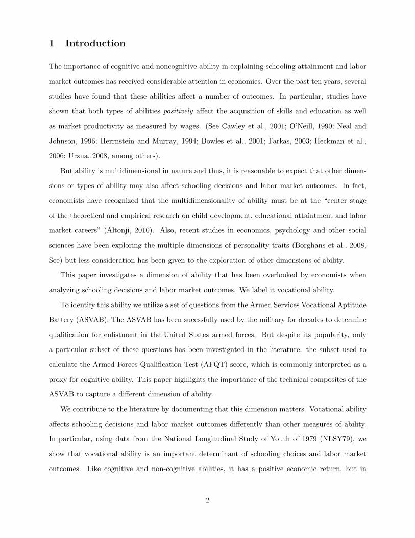
Although the questions answered by the respondents of the NLSY79 are not available, in Figure

1 we present sample questions from the mechanical comprenhension section to have a concrete idea

of the questions. The other sections are similar but include specific terms and devices.2

Relationship with Standard Measures of Ability

In order to establish the relationship between vocational ability and the standard measures of

ability we analyze the correlation between the abilities. Then using Exploratory Factor Analysis-

EFA- we show that two factors are needed in order to explain the correlations observed among the

different components of the ASVAB, those used to compute cognitive ability and those in the three

sections of the ASVAB capturing vocational ability.

The scores in the questions from the three technical composites of the ASVAB are highly cor-

related with the scores in the questions used to compute AFQT - a standard measure of cognitive

ability, and present a low correlation with a standard measure of noncognitive ability. The correla-

tion matrix is presented in Table 1. We show the correlation with AFQT as well as the correlation

with each of the six components used to calculate it: arithmetic reasoning, word knowledge, para-

graph comprehension and math knowledge. For the noncognitive ability we present a standard

measure which is the standardized average of the Rosenberg Self-Esteem Scale and The Rotter

1In the empirical analysis we will control for the effect of education at the time of the test by using the youngestcohort of the survey

2Appendix 8.2 presents an extended list of sample questions for each of the sections used in the analysis.

5

Internal Locus of Control Scale.

Table 1 evidences the high and positive correlation with the standard measure of cognitive

ability, ranging between 0.24 and 0.66. In contrast, the correlation with standard measures of

noncognitive abilities is relatively low, between 0.18 and 0.21. This finding is consistent with modern

psychological theory that views ability as multidimensional while acknowledging that the many

different abilities are themselves positively correlated (Dickens, 2008). This positive correlation

across abilities could be a manifestation of a general ability, sometimes referred as “Spearman g”

or g-factor, or it can well be the result of some overlapping in the knowledge required to answer

the tests.3

[ Table 1 about here ]

In any case, further analysis of the correlation among the variables used to create AFQT and the

technical composites highlights the presence of two different components. In fact, after performing

an Exploratory Factor Analysis (EFA) using nine subsections of the ASVAB, the three technical

composites plus the four set of questions used to create the AFQT, at least two factors are needed

to linearly reconstruct the original variables. In other words, a second factor is needed to explain

the correlation among the scores in the nine questions.4

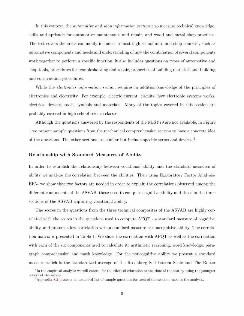
In addition, the estimated loadings suggest a structure of the data where the first factor is

present in all questions but the second factor is only relevant for the three technical composites of

the ASVAB. Figure 2 presents the estimated loadings for each factor, i.e., the estimated coefficients

associated with each factor.

The loadings for the first factor are all positive and ranging between 0.62 and 0.83. In contrast,

the loadings for the second factor differ between the questions used to compute the vocational

ability measure and the questions used to compute AFQT. In particular, the loadings are positive

for the three tests used to construct “Vocational” ranging between 0.31 and 0.48 while non-positive

for the rest, ranging between 0 and -0.38.

3Specifically the fact that all the questions in the three composites of the ASVAB require a certain degree ofreading or verbal comprenhension or that many of the problems require basic mathematics skills.

4In fact, the factor analysis assuming orthogonal factors and allowing for some unique components in the equationkeeps the four first factors, because the default criteria is to keep all the factors with positive eigenvalues. Theeigenvalue for the first factor is 4.75 and 0.80, 0.22 and 0.17 for the next three factors. The first two factors accountfor the shared variance, 87 percent the first and 15 percent the second, so we focus only on them.

6

So, the first factor is capturing all the common information that is expressed by the high

positive correlation among the tests and the second factor captures the additional component that

makes AFQT different from the measure of Vocational ability. The magnitude of the loading is

critical because any factor loading with an absolute value of .30 or greater is considered significant

(Diekhoff, 1992; Sheskin, 2004, among others). Panel a) in Figure 2 presents the original estimated

loadings.

Furthermore, the suggested structure persists also after several forms of rotation. Rotation is

important because of the indeterminacy of the factor solution in the exploratory factor analysis.

In panel b) of Figure 2 we present the loadings after a rotation made to maximize the variance of

the squared loadings between variables (simplicity within factors).

Again, all the loadings for the first factor are significant but for the second factor only the

loadings of the questions used to measure vocational ability are statistically significant. The result

reinforces the structure suggested by the initial factor analysis where the cognitive measures depend

only on the first factor and vocational measures depend on both the first and the second factor.

[Figure 2 about here ]

In this context, the first factor, which is the factor that all composites of the ASVAB have in

common, could be related with the cognitive ability that AFQT is supposed to measure. At the

end, the questions in the three composites of the ASVAB require a certain degree of reading or

verbal comprenhension and many of the problems require basic mathematics skills.

On the other hand, the second factor, the factor that is only present for the technical composites,

may be related to the ability of understanding how things work, a range of skills that makes a person

good performing manual tasks.

In fact, according to Bishop (1988)5 the universe of skills and knowledge sampled by the me-

chanical comprehension, auto and shop information and electronics subtests of the ASVAB roughly

corresponds to the vocational fields of trades and industry and technical so these subtests are inter-

preted as indicators of competence in these areas. ASVAB subtests should be viewed as measures of

5Studied the three components of the ASVAB used here and compared them with occupation specific competencyexaminations that have been developed by the National Occupational Competency Testing Institute and by the statesof Ohio and New York to assess the performance of their high school vocational students. He finds that ASVABitems are from a broader domain than competency tests for individual occupations and individual items appear tobe somewhat more generic. So the different between the two test lies not in the nature of the items but rather intheir difficulty and in the breadth of the occupational knowledge universe from which they are drawn.

7

knowledge, trainability and generic competence for a broad family of jobs involving the operation,

maintenance and repair of complicated machinery and other technically oriented jobs.

If we want to describe a trilogy of abilities that are rewarded in the labor market we can say

that cognitive abilities capture conceptual and thinking skills, while noncognitive/socio-emotional

skills capture human relations skills ,people skills and vocational would be more related to technical

skills how-to-do-it skills.

After presenting the evidence supporting the hypothesis of the existence of a third dimension of

ability that could be captured by the the technical composites of the ASVAB, in the next section

we show the impact of vocational ability on the outcomes of interest: schooling decisions and labor

market outcomes.

3 Impact of Vocational Ability on Outcomes

This section presents the data used and the reduced-form estimations of the implied behavior

of vocational ability in terms of schooling choices and wages unconditional and conditional on

standard measures of ability. The insights from the descriptive analysis are used in two ways.

First, to document that the measure of vocational ability is correlated with schooling decisions

differently than standard measures of ability. Second, to motivate the use of the model to capture

the effect of vocational abilty overcoming the main problems associated with the reduced-form

approach.

3.1 Data

The National Longitudinal Survey of Youth (NLSY) is a panel data set of 12,686 individuals

born between 1957 and 19646. This survey is designed to represent the population of youth aged

14 to 21 as of December 31 of 1978, and residing in the United States on January 1, 1979. It

consists of both a nationally representative cross-section sample and a set of supplemental samples

designed to oversample civilian blacks, civilian Hispanics, economically disadvantaged Non-Black/

Non-Hispanic youths and individuals in the military. Data is collected in an annual basis from 1979

to 1994 and biannually until 2010.

62,439 white males-21 percent of total surveyed individuals and 40 percent of the individuals in the cross-sample

8

We use the cross-section sample of white males between the ages of 25 and 30 who were not

attending school at the time of the survey and who were up to high school graduates by the time

the tests were collected. We chose to analyze white males in order to have a benchmark to compare

our results with previous studies (Heckman et al., 2006; Neal and Johnson, 1996, etc). In addition,

we want to abstract from influences that operate differently on various demographic groups. In

consequence, our analysis is specific and cannot be generalized to the whole population.

The age selection responds to the interest of analyzing entry level wages abstracting from the

cummulative effects of ability on experience and tenure. At age 25 more than 97 percent of the

sample has reached their maximum level of education. The five-years window is useful to get an

smooth average if the first part of the wage profile of the individuals.

From the original sample of 12,686 individuals, 11,406 are civilian, 6,111 belong to the cross-

section sample. Nearly 49 percent of that sample are males (2,438 individuals), 1,999 had less than

high school complete by the time the ASVAB test was conducted (Summer 1980) , out of them just

1,832 individuals are observed at least once between the ages of 25 and 30 and finally, 1,710 were

not attending school by the time the survey was conducted. That sample is further reduced for the

analysis accordig to the variables of interest. We get rid of 230 observations that either are high

school dropouts or have no information on schooling. Also 59 individuals were excluded because

they have no information on average wage. In addition, 67 individuals were removed due the lack

of information on test scores so we end up with a sample of 1,354 individuals. Table 2 presents the

description of the variables used.

[Table 2 here]

We analyze one schooling choice, 4 year college attendance. The variables used to determine

college attendance are maximum degree attained by age 25 and type of college enrolled. The labor

market outcome of interest is the log of the average of the hourly wages reported between 25 and

30 years old. For the cognitive and vocational measures we rely on the Armed Service Vocational

Aptitude Battery (ASVAB)7 that was conducted in the summer and fall of 1980. This test was

administrated to over 90 percent of the members of the NLSY panel. (Individuals had between 15

and 23 years old at the time of the test) The test is conformed by a battery of 10 questions with the

7these questions are used to compute the AFQT that is used by the military services for enlistment screeningand job assignment within the military.

9

objective of measure knowledge and skills in the following areas: general science, arithmetic rea-

soning, word knowledge, paragraph comprehension, numerical operations, coding speed, auto and

shop information, mathematics knowledge, mechanical comprehension and electronics information.

For the noncognitive ability measurements we use two test: a) Rotter Locus of Control Scale

and b) the Rosenberg Self-Esteem Scale. The Rotter Locus of Control Scale measures the degree

of control individuals feel they possess over their life. In 1979 the NLSY collected a total of four

items selected from the 23-item forced choice questionnaire adapted from the 60-item Rotter Adult

I-E scale developed by Rotter (1966). “This scale was designed to measure the extent to which

individuals believe they have control over their lives through self-motivation or self-determination

(internal control) as opposed to the extent that the environment (that is, chance, fate, luck) controls

their lives (external control). The scale is scored in the external direction-the higher the score, the

more external the individual”.8

The Rosenberg Self-Esteem Scale which based on 10 questions measures only self-esteem. “It

describes a degree of approval or disapproval toward oneself (Rosenberg, 1965). The scale is short,

widely used, and has accumulated evidence of validity and reliability. It contains 10 statements of

self-approval and disapproval with which respondents are asked to strongly agree, agree, disagree,

or strongly disagree. The scale has proved highly internally consistent, with reliability coefficients

that range from .87 (Menaghan, 1990) to .94 (Strocchia-Rivera, 1988), depending on the nature of

the NLSY79 sample selected.”9.

Distributions

The tests are used to create a composite measure for each type of ability. For cognitive ability

the measure is constructed using an average of the standardized scores for arithmetic reasoning,

mathematical knowledge, paragraph comprenhension,word knowledge, numerical operations and

coding speed. For noncognitive ability the measure is created as the sum of the average of Rotter

and Rosenberg scores. Finally, vocational ability measuremente is constructed as the average of

the standardized scores in mechanical comprenhension, electronics information and auto and shop

information.

8Extracted from http://www.nlsinfo.org/nlsy79/docs/79html/79text/attitude.htm9Extracted from http://www.nlsinfo.org/nlsy79/docs/79html/79text/attitude.htm

10

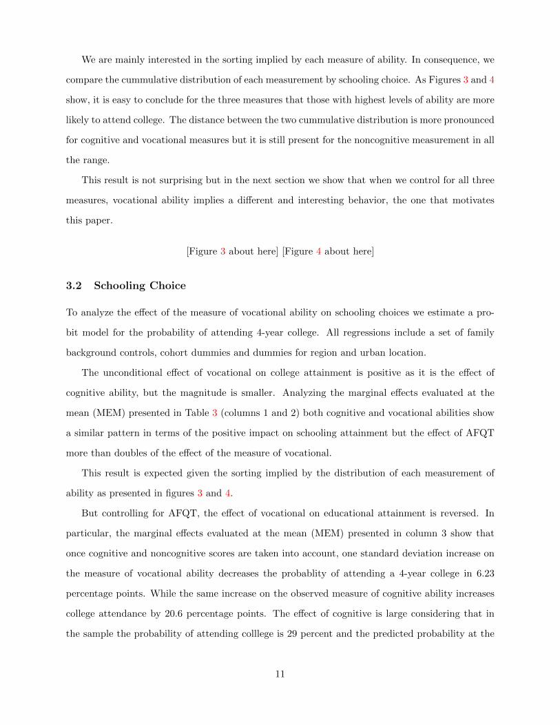
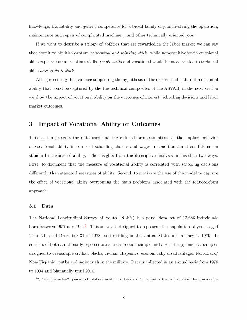
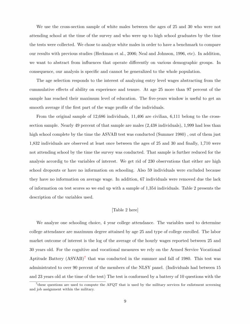
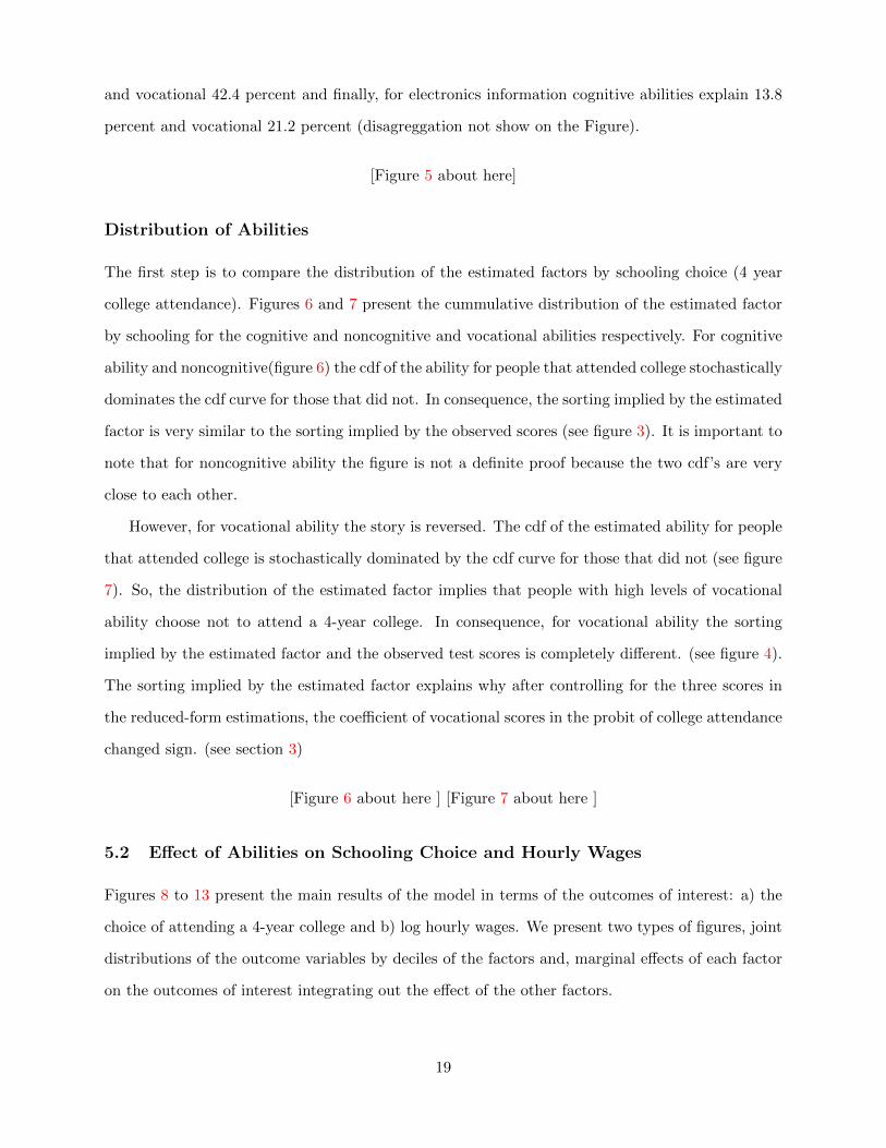
We are mainly interested in the sorting implied by each measure of ability. In consequence, we

compare the cummulative distribution of each measurement by schooling choice. As Figures 3 and 4

show, it is easy to conclude for the three measures that those with highest levels of ability are more

likely to attend college. The distance between the two cummulative distribution is more pronounced

for cognitive and vocational measures but it is still present for the noncognitive measurement in all

the range.

This result is not surprising but in the next section we show that when we control for all three

measures, vocational ability implies a different and interesting behavior, the one that motivates

this paper.

[Figure 3 about here] [Figure 4 about here]

3.2 Schooling Choice

To analyze the effect of the measure of vocational ability on schooling choices we estimate a pro-

bit model for the probability of attending 4-year college. All regressions include a set of family

background controls, cohort dummies and dummies for region and urban location.

The unconditional effect of vocational on college attainment is positive as it is the effect of

cognitive ability, but the magnitude is smaller. Analyzing the marginal effects evaluated at the

mean (MEM) presented in Table 3 (columns 1 and 2) both cognitive and vocational abilities show

a similar pattern in terms of the positive impact on schooling attainment but the effect of AFQT

more than doubles of the effect of the measure of vocational.

This result is expected given the sorting implied by the distribution of each measurement of

ability as presented in figures 3 and 4.

But controlling for AFQT, the effect of vocational on educational attainment is reversed. In

particular, the marginal effects evaluated at the mean (MEM) presented in column 3 show that

once cognitive and noncognitive scores are taken into account, one standard deviation increase on

the measure of vocational ability decreases the probablity of attending a 4-year college in 6.23

percentage points. While the same increase on the observed measure of cognitive ability increases

college attendance by 20.6 percentage points. The effect of cognitive is large considering that in

the sample the probability of attending colllege is 29 percent and the predicted probability at the

11

mean of the observed variables is 22.6.

[Table 3 about here]

3.3 Hourly Wages

Analyzing hourly wages, the return to the score in the vocational measure is positive and high, even

when compared to the return to AFQT In particular, controlling for education, one unit increase

in vocational is associated with a 3,58 percent increase in the level of hourly wages. The effect is

even bigger than the effect of noncognitive test scores, although less precise. The effect of cognitive

scores on wages is more than twice this value.

[Table 4 here]

So far the regressions show that vocational abilities are rewarded by the labor market but imply

a different behavior. Those regressions are problematic because 1) schooling choices are endogenous

and that must be controlled for if to estimate the returns to unobserved heterogeneity and 2) Test

scores are just proxies of abilities and they are influenced by schooling, age and family background

variables. The next section presents the model proposed to measure more accurately the effect of

vocational ability.

4 Model: Augmented Roy Model with Factor Structure

The model presented in this section deals with two of the main problems associated with conven-

tional analysis: The endogeneity of schooling choices and the fact that test scores are just proxies

of abilities and they are influenced by schooling, age and family background variables.

In this context, the strategy pursued in this paper is based on a model that integrates wages

with schooling decisions and wages. The model proposed follows closely the models presented

in Heckman et al. (2006) and Urzua (2008) where a vector of low dimensional factors, latent

cognitive and noncognitive abilities, is used to generate the distribution of potential outcomes.

These latent abilities generate measured cognitive, noncognitive and vocational scores and the rest

of the outcomes analyzed and in this setting are the only source of dependence among all equations.

12

The theoretical model is static and does not consider the timing of the decisions. As a result, the

schooling choice model is evaluated at age 25-30. Agents choose their maximum level of schooling

before age 25 given the information they have at the time. We assume that the latent abilities

are unobserved but the individual has full information about his/her abilities, as well as how they

affect the potential earnings in each selection. The agent compares the outcomes in each selection

and chooses the alternative that yields a higher payoff.

Each of the components of the model will be presented in a separate subsection of the present

section. The model we estimate uses 2 schooling levels (Attended 4-year college or not), 3 factors,

6 cognitive tests, 3 tests on vocational ability and 2 tests on noncognitive abilities. We assume

normality on the error terms which is neither necessary, nor important for the proceding analyses.

4.1 Model of Schooling Choices

The latent utility of getting education is given by:

D = 1[Ii > 0]

Ii = XD,iβD + λcDθc,i + λvDθv,i + λnDθn,i + ei for i = 1, ...N

ei ∼ N(0, 1)

where Xi is a matrix of observed variables that affect schooling, βs is the vector of coefficients.

The vector of latent factors is given by θ = [θc,i, θv,i, θn,i] where subscript c is used to denote the

cognitive ability, subscript v vocational ability and subscript n noncognitive ability. λcD, λvD, λ

nD,

are the coefficients associated with the cognitive, vocational and noncognitive latent abilities, re-

spectively. These coefficients are referred in the literature as the factor loadings. ei is the error

component that is assumed to be independent of XD, θ and following a standard normal distribu-

tion. Then D denotes a binary variable that takes the value of 1 if the individual chooses to attend

a 4-year college and 0 otherwise.10

Conditional on XD and θ equations produce a standard discrete choice model with a factor

structure. Furthermore, given the set of assumptions exposed, this can be interpreted as the

10Through all the exposition the indicator function will be used, 1[] this function takes a value of one if thecondition inside the parentheses is satisfied.

13

standard probit model.

4.2 Model of Hourly Wages

Analogously, the model of earnings can be expresed as a linear function of Xw,i and θ in the

following way:

lnwD,i = Xw,iβw,D + λcw,Dθc,i + λvw,Dθv,i + λnw,Dθn,i + ew,D,i

ew,D,i ∼ N(0, 1)

for D = 0, 1

4.3 Model of Test Scores: Measurement System

Motivated for the findings of the Exploratory Factor Analysis performed in section 2 the model of

test scores allow each measurement to be a function of the corresponding latent ability but in the

case of the measurements of vocational ability we allow them to be a function of both cognitive

and vocational latent factors.

In this context, the model for the cognitive measure Cj is:

Cj,i = XCj ,iβCj + λcCjθc,i + eCj ,i

for j = 1, ..., 6

The model for the vocational measure Vl is:

Vk,i = XVk,iβVk+ λcVk

θc,i + λvVkθv,i + eVk,i

for k = 1, ..., 3

And the model for the noncognitive measure Nl is:

Nl,i = XNl,iβNl+ λnNl

θn,i + eNl,i

14

for l = 1, 2

Finally, all error terms ei, eC1,i, ..., eC6,i, eV1,i, ..., eV3,i, eN1,i, eN2,i for D = 0, 1,j = 1, ..., 6 , k =

1, ..., 3 are mutually independent, independent of the factors and independent of all observable

characteristics. This independence is essential to the model since it implies that all the correlation

in observed choices and measurements is captured by latent unobserved factors.

4.4 Latent Factors

The level of these factors may be the result of some combination of inherited ability, the quality of

the family environment in which individuals were raised, cultural differences, etc. These factors are

assumed to be fixed by the time the individual is choosing the level of education and thus, by the

time the labor and behavioral outcomes considered in this document are determined. In addition,

the factors are assumed to be known by the individual but unknown to the researcher and mutually

independent, θc ⊥ θv ⊥ θn.

A mixture of normals is used to model the distribution of the latent abilities. This distribution

is selected because as Ferguson (1983) proved, a mixture of normals can approximate any distri-

bution, and we will like to impose the minimum number of restrictions on the distribution of these

unobserved components.

θc,i ∼∑K

k=1 pkN(µkc ,(σkc)2)

θv,i ∼∑M

m=1 pmN(µmv , (σ

mv )2)

θn,i ∼∑L

l=1 plN(µln,(σln)2)

with

M∑m=1

pm =K∑k=1

pk =L∑l=1

pl = 1

In this case, we use mixtures of 2 normals so K = L = M = 2

and

15

E[θc] = E[θv] = E[θn] = 0

4.5 Estimation Strategy

This section contains a brief explanation of the estimation strategy.

Likelihood Function

Let Ti = {C1i, ..., C6,i, V1i, ..., V3,i, N1i, N2,i}, be the vector of test scores for individual i. Let

θ = [θc, θv, θn] be the vector of the latent factors and δ the vector of all the parameters of the model

L(δ|X) =

N∏i=1

f(Di, lnwD,i, Ti|Xi, Xw,i, XT,i)

Given that conditional on unobserved endowments all the errors are mutually independent this

can also be expressed as:

L(δ|X) =N∏i=1

∫Θ

f(Di, lnwD,i, Ti|Xi, Xw,i, XT,i, θ)dF (θ)

where

f(Di, lnwD,i, Ti|Xi,Xw,i, XT , θ) = f(Di, lnwD,i|Xi, Xw,i, θ)f(Ti|XT,i, θ)

f(Di, lnwD,i|Xi, Xw,i, θ) = (Pr(Di = 1|Xi, θ)f(lnw1,i|Di = 1, Xw,i, θ))Di

× (Pr(Di = 0|Xi, θ)f(lnw0,i|Di = 0, Xw,i, θ))1−Di

with

Pr(Di = 1|Xi, θ) = Pr (XiβD + λcDθc,i + λvDθv,i + λnDθn,i + ei ≥ 0)

= Φ (−XiβD − λcDθc,i − λvDθv,i − λnDθn,i)

16

and

f(lnwD,i|Di, Xw,i, θ) = φ(lnwD,i −Xw,iβw,D + λcw,Dθc,i + λvw,Dθv,i + λnw,Dθn,i + ew,D,i

)

f(Ti|XT,i, θ) =6∏

j=1

f(Cj,i|XT , θc)×3∏

k=1

f(Vk,i|XT , θc, θv)×2∏

l=1

f(Nl,i|XT , θn)

with

f(Cj,i|XT , θc) = φ(Cj,i −XCj ,iβCj − λcCj

θc,i

)for j = 1, ..., 6

f(Vk,i|XT , θc, θv) = φ(Vk,i −XVk,iβVk

− λcVkθc,i − λvVk

θv,i)

for k = 1, ..., 3

f(Nl,i|XT , θn) = φ(Nl,i −XNl,iβNl

− λnNlθn,i)

for l = 1, 2

We are computing the sample likelihood using Bayesian MCMC methods. The use of Bayesian

methods is only for computational convenience, in order to avoid the computation of the integral.

For details Hansen et al. (2004) and Heckman et al. (2006).

5 Results and Discussion

Given the nonlinear and multidimensional nature of the model, the best way to understand the

results is through simulation. We first compare the distribution of the estimated factors with the

observed distribution of the measurements. Then we summarize the main results of the model in

a series of figures.

Our results confirm the results from the reduced form. Vocational ability in fact reduces the

probability of seeking a professional degree and at the same time is positively rewarded in the labor

17

market. Using simulations we can explore the implications of being low in the standard types of

ability but having high levels of vocational ability in terms of schooling choices and earnings.

5.1 Observed Test Scores and Estimated Abilities

As explained in Section 4.3, this paper treats observed cognitive, noncognitive and vocational test

scores as the outcomes of a process that has as inputs family background, schooling at the time

of the test and unobserved abilities. Table 5 presents the loadings for each of the tests. For

identification purposes one loading for each unobserved ability is set to one so the rest of the

loadings are interpreted in relation to the loading set as numerarie (for details see Carneiro et al.,

2003). The selected numeraries are Mathematical Knowledge, Mechanical Comprenhension and

the Rosenberg self-esteem scale for cognitive, vocational and noncognitive abilities respectively.

[ Table 5 about here]

To analyze the relative importance of each unobserved ability in explaining test scores, Figure 5

presents the variance decomposition of the measurement system. The results show the contribution

of observed variables, latent abilities and error terms as determinants of the variance of each test

score.

The first observation is the very low contribution of observed variables to the variance of the

test scores. It never explains more than 20 percent. This evidences the large size of the unexplained

component and highlights the implications of using observed test scores to proxy for unobserved

abilities. After controlling for the latent variables, the error term is still large but we are able to

explain a higher percentage of the total variance, between 34 and 65 percent, except for the Rotter

Scale in which case we are not able to explain more than 11 percent of the variance.

It is important to note that for the three vocational tests (Auto, Mech. C and Electronics)

we allow both cognitive and vocational abilities to influence the scores. While cognitive ability

has lower loadings compared to vocational ability (see Table 5), in the variance decomposition we

confirm that both abilities are important to explain the variance.

In particular, for mechanical comprenhension cognitive explains 14 percent of the variance

while vocational explains 17 percent. For auto shop information vocational explains 12.6 percent

18

and vocational 42.4 percent and finally, for electronics information cognitive abilities explain 13.8

percent and vocational 21.2 percent (disagreggation not show on the Figure).

[Figure 5 about here]

Distribution of Abilities

The first step is to compare the distribution of the estimated factors by schooling choice (4 year

college attendance). Figures 6 and 7 present the cummulative distribution of the estimated factor

by schooling for the cognitive and noncognitive and vocational abilities respectively. For cognitive

ability and noncognitive(figure 6) the cdf of the ability for people that attended college stochastically

dominates the cdf curve for those that did not. In consequence, the sorting implied by the estimated

factor is very similar to the sorting implied by the observed scores (see figure 3). It is important to

note that for noncognitive ability the figure is not a definite proof because the two cdf’s are very

close to each other.

However, for vocational ability the story is reversed. The cdf of the estimated ability for people

that attended college is stochastically dominated by the cdf curve for those that did not (see figure

7). So, the distribution of the estimated factor implies that people with high levels of vocational

ability choose not to attend a 4-year college. In consequence, for vocational ability the sorting

implied by the estimated factor and the observed test scores is completely different. (see figure 4).

The sorting implied by the estimated factor explains why after controlling for the three scores in

the reduced-form estimations, the coefficient of vocational scores in the probit of college attendance

changed sign. (see section 3)

[Figure 6 about here ] [Figure 7 about here ]

5.2 Effect of Abilities on Schooling Choice and Hourly Wages

Figures 8 to 13 present the main results of the model in terms of the outcomes of interest: a) the

choice of attending a 4-year college and b) log hourly wages. We present two types of figures, joint

distributions of the outcome variables by deciles of the factors and, marginal effects of each factor

on the outcomes of interest integrating out the effect of the other factors.

19

Figures 8 and 9 present the joint distribution of the probability of attending a 4-year college

reported by deciles of cognitive and vocational and then by the deciles of noncognitive and voca-

tional. The opposite effects of the abilities are evident but the positive effect of cognitive is always

stronger, as measured by the slope of the log wage-cognitive decile curve. As en exercise we can

move along the distributions and compare the effect of increasing one decile on both cognitive and

vocational on the probability of going to college. Given that cognitive has a positive effect and

vocational a negative effect this exercise will show which effect prevails. Starting at the lowest

extreme of both distributions (first decile of both cognitive and vocational) and moving to the next

decile of the distributions of both cognitive and vocational abilities the estimated probability of

going to college always increases.

A similar exercise on the distributions of noncognitive and vocational proves the pattern ob-

served in Figure 9, where the negative effect of vocational always outweighs the positive effect of

noncognitive.

The marginal effect of cognitive integrating out the effect of vocational is presented in panel

a of Figure 10 while panel b and c present the analogous for noncognitive and vocational ability,

respectively.

In addition, our results present smaller effects of the factors on schooling, in absolute values,

compared with the results from the reduced form in Section 3. Specifically, according to our

estimates, one standard deviation increase in cognitive ability is associated with an increase of

14.6 percentage points in the probability of attending 4-year college (17.3 pp from the reduced-

form) while one standard deviation increase in vocational ability decreases the probability in 5.8

percentage points (3.8 pp in the reduced-form) and the effect of noncognitive is 1.5 pp in both the

results from the model and the reduced-form.

[Figure 8 about here] [Figure 9 about here] [Figure 10 about here] [Table 6 about here]

Figures 11 and 12 display the total effect of ability on log wages, including the direct effect of

ability on log wages holding schooling constant, the effect of ability on the decision to attend college

and the implied effect of attending or not college on log wages. The effect of all abilities is positive

but the effect of vocational is considerable small compared with cognitive and noncognitive. In

fact, the effect of one standard deviation increase in cognitive ability is associated with 9.4 percent

20

increase in log hourly wages and 3.8 for noncognitive ability. The average estimated effect of

vocational is 1.2 percent panels a,b and c of Figure 13 present the marginal effect of cognitive,

noncognitive and vocational abilities on the log wage.

[Figure 11 here] [Figure 12 here] [Figure 13 here]

5.3 Sorting and Comparative Advantage

Vocational ability implies a different behavior and has a positive, although small, average reward

on the labor market. In this section we investigate the effect further. On the one hand, we estimate

average results in terms of sorting and comparative/ vs absoulte advantage and on the other hand

we further investigate the effect vocational ability on wages for different combinations of abilities.

In particular, we are interested in understand what are the implications of having low levels of

cognitive and noncognitive abilities but high levels of vocational abilities in terms of hourly wages.

In the context of our model, the sorting into schooling levels is analyzed with the following

question: Are the earnings for those who decided to attend college higher of lower than they would

be if assignment to schooling were random? So we will refer to positive sorting the case where the

difference between the conditional and the unconditional mean of earnings is positive.

E[Y1|D = 1]− E[Y1] > 0

E[Y0|D = 0]− E[Y0] > 0

Regarding the analysis of comparative advantage it is important to highlight the essential

departure of our model from the typical versions of the Roy model. Even in the multiple-index Roy

model, workers have unobserved talent components, but they can only use one in each scenario

(college/ no college). Hence, workers self-select into the schooling level that gives them the highest

expected earnings. Equilibrium in each market equates supply and demand, while a self-selection

condition means that the marginal worker is indifferent between the two sectors. In our specification

the unobserved talent has three components: cognitive, vocational and noncognitive and all three

are used in each scenario. In this context, we analyze comparative advantage comparing the

21

conditional mean of hourly wages with the respective counterfactual. In particular, we compute

the following differences:

E[Y1|D = 1]− E[Y0|D = 1]

E[Y0|D = 0]− E[Y1|D = 0]

[Table 7 here]

According to the results presented in Table 7 we observe on average positive sorting into college

attendance. In fact, the earnings for those who decided to attend college are 6.8 percent higher

than they would be if assignment to schooling were random. Also, we find evidence of comparative

advantage since the mean of hourly wages conditional on college attendance in 9.3 percent higher

than the respective counterfactual- earnings that would have been received in the scenario where

the individual decided not attending to college.

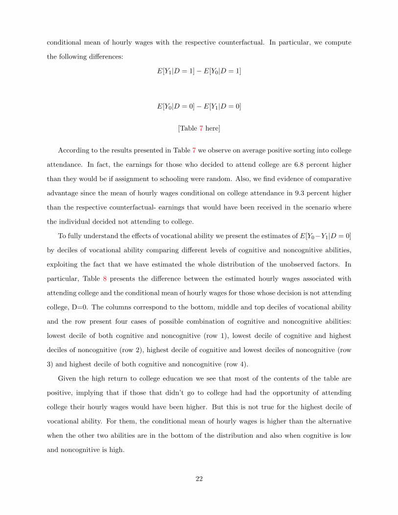
To fully understand the effects of vocational ability we present the estimates of E[Y0−Y1|D = 0]

by deciles of vocational ability comparing different levels of cognitive and noncognitive abilities,

exploiting the fact that we have estimated the whole distribution of the unobserved factors. In

particular, Table 8 presents the difference between the estimated hourly wages associated with

attending college and the conditional mean of hourly wages for those whose decision is not attending

college, D=0. The columns correspond to the bottom, middle and top deciles of vocational ability

and the row present four cases of possible combination of cognitive and noncognitive abilities:

lowest decile of both cognitive and noncognitive (row 1), lowest decile of cognitive and highest

deciles of noncognitive (row 2), highest decile of cognitive and lowest deciles of noncognitive (row

3) and highest decile of both cognitive and noncognitive (row 4).

Given the high return to college education we see that most of the contents of the table are

positive, implying that if those that didn’t go to college had had the opportunity of attending

college their hourly wages would have been higher. But this is not true for the highest decile of

vocational ability. For them, the conditional mean of hourly wages is higher than the alternative

when the other two abilities are in the bottom of the distribution and also when cognitive is low

and noncognitive is high.

22

This suggests that individuals with very high levels of vocational ability but low levels of

cognitive ability not going to college is associated with the highest expected hourly wage.

[Table 8 here]

6 Conclusions

In this paper we explore vocational ability as a particular dimension that has received little attention

by economists when analyzing the effect of abilities on schooling choices and labor market outcomes.

We show that like standard measures of ability, vocational ability is positively rewarded by the labor

market, but that in contrast to these other measures, vocational ability predicts the choice of low

levels of schooling. In particular, controlling for standard measures, it reduces the likelihood of

attending college.

In this context, vocational ability enriches the current measures of the heterogeneity that ex-

plains differences in wages and expands current knowledge on the composition of human capital.

In particular, including vocational ability in the analysis implies a transition from the dichotomy

between low vs high ability workers (skilled vs unskilled) to a new framework where individuals

with low cognitive and noncognitive abilities could have high vocational ability and greatly benefit

from it.

For this reason, the question studied in this paper is does vocational ability affect schooling

decisions and labor market outcomes differently than other measures? If so, what is the implication

of having low abilities under the standard definition, but high vocational ability?

Using information on white males from the NLSY79 and a Roy model with factor structure we

are able to show that for individuals with very high levels of vocational ability but low levels of

standard ability (cognitive and noncognitive), not going to college is associated with the highest

expected hourly wage, despite the high returns associated with college. More specifically, the mean

of hourly wages conditional on not going to college is higher than the counterfactual corresponding

to the scenario of going to college.

The latter result is a consequence of the fact that the returns to vocational ability are higher

compared to returns to cognitive ability conditional on not going to college and that the returns to

vocational conditional on going to college are considerably lower than the returns conditional on

23

not going to college.

In conclusion, the paper presents a new dimension of ability that is important and can be mea-

sured with standard tests that are readily available. The new dimension allows us to characterize

in more detail the heterogeneity of workers. Furthermore, we find a group of workers that despite

the high returns to college actually benefit from not going to college. Those individuals would

not benefit from a policy of ”College for All” but would benefit from a type of education that

potentializes their vocational ability to exploit the large returns to it.

24

Figure 1: Sample question from the mechanical comprenhension section

a

1. In the diagram, what can you tell about the load on posts A and B?

(a) Post B carries more weight.

(b) Post A carries more weight.

(c) Post A carries no weight.

(d) The load is equal on posts A and B.

2. The diagram shows a class 1 lever. Which of the following is the same kind of lever?

(a) A pair of tweezers

(b) A pair of scissors

(c) A wheelbarrow

(d) A pair of tongs

3. Which of the following would feel hottest to the touch if one end were placed in a pot of boiling water?

(a) A wooden spoon

(b) A metal fork

(c) A plastic knife

(d) A plastic cup

aExtracted from http://www.education.com/reference/article/mechanical-comprehension-quiz/

25

7 Tables and Figures

Table 1: Correlation of the Technical Composites of the ASVAB with Tests Used to CreateAFQT (cognitive) and a Composite Measure of Noncognitive

Auto Mech Elect AFQT Arith Coding Math Word Parag Num Nocog

Auto 1.00

Mechanical. C 0.65 1.00

Electronics 0.64 0.66 1.00

AFQT 0.40 0.55 0.56 1.00

Arithmetic K. 0.40 0.60 0.54 0.80 1.00

Coding S. 0.27 0.37 0.35 0.83 0.49 1.00

Math 0.25 0.50 0.47 0.79 0.77 0.50 1.00

Word K. 0.50 0.55 0.66 0.74 0.61 0.45 0.59 1.00

Paragraph C. 0.41 0.53 0.56 0.73 0.63 0.46 0.59 0.73 1.00

Numerical S. 0.24 0.34 0.36 0.84 0.58 0.65 0.65 0.49 0.51 1.00

NoCognitive 0.18 0.21 0.21 0.26 0.23 0.18 0.18 0.29 0.24 0.20 1.00

Note: AFQT is the cognitive measure, it represents the standardized average over the ASVAB score in six of the ten

components: math knowledge, arithmetic reasoning, word knowledge, paragraph comprehension, numerical speed and coding

speed. Noncognitive is the standardized average of the scores for the Rotter and Rosenberg tests.

26

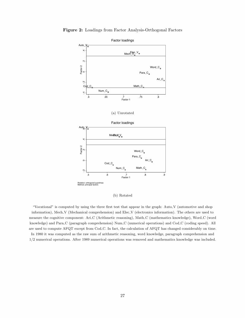
Figure 2: Loadings from Factor Analysis-Orthogonal Factors

Auto_V

Mech_VElec_V

Ari_C

Math_C

Word_C

Para_C

Cod_CNum_C

-.4-.2

0.2

.4Fa

ctor

2

.6 .65 .7 .75 .8Factor 1

Factor loadings

(a) Unrotated

Auto_V

Mech_VElec_V

Ari_C

Math_C

Word_C

Para_C

Cod_C

Num_C

-.20

.2.4

.6Fa

ctor

2

.5 .6 .7 .8 .9Factor 1

Rotation: orthogonal quartimaxMethod: principal factors

Factor loadings

(b) Rotated

“Vocational” is computed by using the three first test that appear in the graph: Auto V (automotive and shop

information), Mech V (Mechanical comprehension) and Elec V (electronics information). The others are used to

measure the cognitive component: Ari C (Arithmetic reasoning), Math C (mathematics knowledge), Word C (word

knowledge) and Para C (paragraph comprehension) Num C (numerical operations) and Cod C (coding speed). All

are used to compute AFQT except from Cod C. In fact, the calculation of AFQT has changed considerably on time.

In 1980 it was computed as the raw sum of arithmetic reasoning, word knowledge, paragraph comprehension and

1/2 numerical operations. After 1989 numerical operations was removed and mathematics knowledge was included.

27

Table 2: Summary statistics

Variable Mean (Std. Dev.) Min. Max. N

LogHourly wage 25-30 2.847 (0.544) 0.628 8.977 1315Attended 4yrcollege by age 25 0.29 (0.454) 0 1 1315Urban residence at age 25 0.75 (0.433) 0 1 1235Northeast residence at age 25 0.188 (0.391) 0 1 1315Northcentral residence at age 25 0.359 (0.48) 0 1 1315South residence at age 25 0.279 (0.449) 0 1 1315West residence at age 25 0.163 (0.37) 0 1 1315Cohort1 (Born 57-58) 0.132 (0.338) 0 1 1315Cohort2 (Born 59-60) 0.194 (0.396) 0 1 1315Cohort3 (Born 61-62) 0.329 (0.47) 0 1 1315Cohort4 (Born 63-64) 0.345 (0.476) 0 1 1315Family Income in 1979 (thousands) 21.669 (11.779) 0 75.001 1315Broken home at age 14 0.195 (0.396) 0 1 1312Number of siblings 1979 2.966 (1.958) 0 17 1315Mother’s highest grade completed 11.309 (3.258) 0 20 1311Father’s highest grade completed 11.459 (3.893) 0 20 1304Living in urban area at age 14 0.725 (0.446) 0 1 1311Living in the south at age 14 0.254 (0.436) 0 1 1297Education at the time of the test 11.211 (1.013) 6 12 1315AFQT 0 (1) -3.193 2.198 1315Vocational 0 (1) -3.196 2.011 1315NonCognitive 0 (1) -2.749 2.517 1315

Notes: AFQT is an average of standarized scores for arithmetic reasoning, word knowledge,paragraph comprehension, mathematics knowledge, numerical operations and coding speed sec-tions of the ASVAB. Noncognitive is an average of the scores in two tests:Rotter Locus of ControlScale and Rosenberg Self-Esteem Scale. Vocational is an average of standarized scores for autoand shop information, mechanical comprehension and electronics information sections of theASVAB.

28

Figure 3: Measurement of Cognitive and Noncognitive Ability

0

.2

.4

.6

.8

1

Den

sity

-3 -2 -1 0 1 2Cognitive Measure

No College College

CDF of Cognitive Measure by College

(a) Cognitive

0

.2

.4

.6

.8

1

Den

sity

-4 -2 0 2Noncognitive Measure

No College College

CDF of Noncognitive Measure by College

(b) Noncognitive

Figure 4: Measurement of Vocational Ability

0

.2

.4

.6

.8

1

Den

sity

-4 -2 0 2Vocational Measure

No College College

CDF of Vocational Measure by College

29

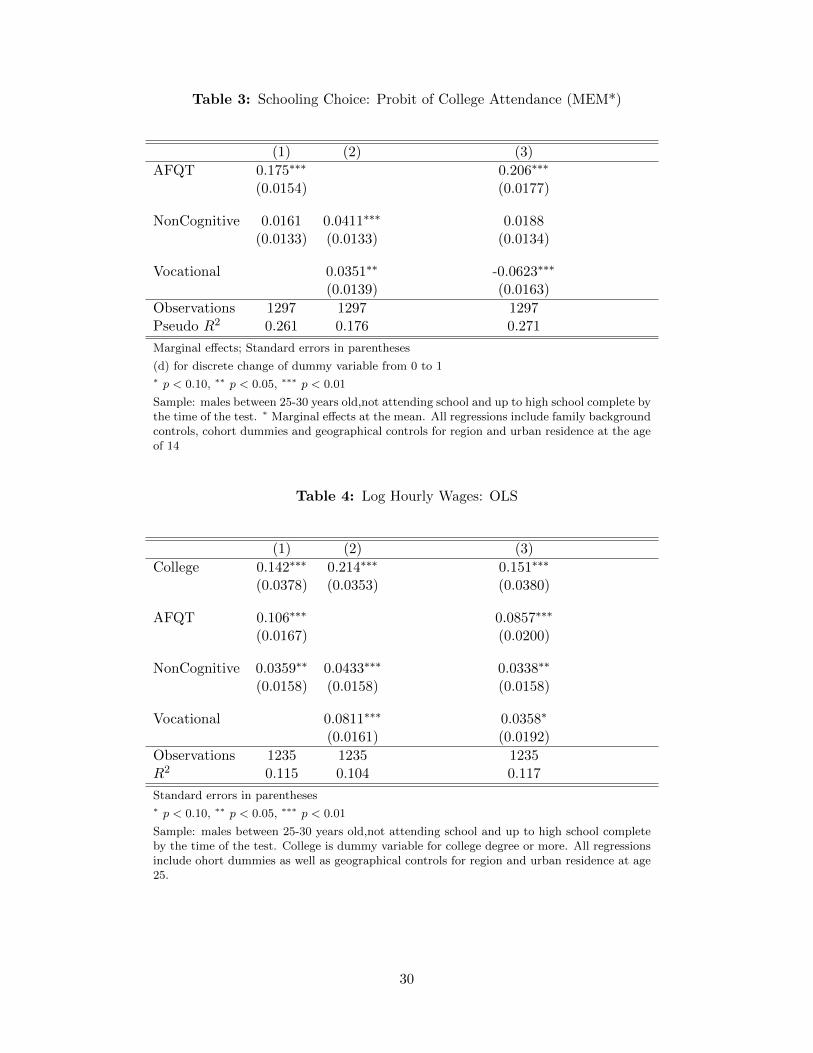
Table 3: Schooling Choice: Probit of College Attendance (MEM*)

(1) (2) (3)

AFQT 0.175∗∗∗ 0.206∗∗∗

(0.0154) (0.0177)

NonCognitive 0.0161 0.0411∗∗∗ 0.0188(0.0133) (0.0133) (0.0134)

Vocational 0.0351∗∗ -0.0623∗∗∗

(0.0139) (0.0163)

Observations 1297 1297 1297Pseudo R2 0.261 0.176 0.271

Marginal effects; Standard errors in parentheses

(d) for discrete change of dummy variable from 0 to 1∗ p < 0.10, ∗∗ p < 0.05, ∗∗∗ p < 0.01

Sample: males between 25-30 years old,not attending school and up to high school complete bythe time of the test. ∗ Marginal effects at the mean. All regressions include family backgroundcontrols, cohort dummies and geographical controls for region and urban residence at the ageof 14

Table 4: Log Hourly Wages: OLS

(1) (2) (3)

College 0.142∗∗∗ 0.214∗∗∗ 0.151∗∗∗

(0.0378) (0.0353) (0.0380)

AFQT 0.106∗∗∗ 0.0857∗∗∗

(0.0167) (0.0200)

NonCognitive 0.0359∗∗ 0.0433∗∗∗ 0.0338∗∗

(0.0158) (0.0158) (0.0158)

Vocational 0.0811∗∗∗ 0.0358∗

(0.0161) (0.0192)

Observations 1235 1235 1235R2 0.115 0.104 0.117

Standard errors in parentheses∗ p < 0.10, ∗∗ p < 0.05, ∗∗∗ p < 0.01

Sample: males between 25-30 years old,not attending school and up to high school completeby the time of the test. College is dummy variable for college degree or more. All regressionsinclude ohort dummies as well as geographical controls for region and urban residence at age25.

30

Table 5: Loadings on Test Scores

Cognitive Vocational Noncognitive

Auto 0.35 *** 1.51 ***Electronics 0.50 *** 0.94 ***Mech. C 0.52 *** 1.00Arithmetic K. 1.03 ***Math 1.00Word K. 0.87 ***Paragraph C. 0.91 ***Numerical S. 0.78 ***Coding S. 0.69 ***Rotter 0.23 ***Rosenberg 1.00

All regressions include family background controls (mother’s and father’s education, numberof siblings, a dummy for broken family at age 14, family income in 1979), cohort dummiesand geographical controls for region and urban residence at the age of 14.

Figure 5: Variance Decomposition

0%   20%   40%   60%   80%   100%  

Rosenberg  

Roter  

Mech.  C  

Arithme:c  K.  

Coding  S.  

Math  

Electronics  

Auto  

Numerical  S.  

Paragraph  C.  

Word  K.  

Observables   Latent  factors   Error  

31

Figure 6: Cognitive and Noncognitive Ability

(a) Cognitive (b) Noncognitive

Figure 7: Vocational Ability

32

Figure 8: Joint Distribution of College Attendance Decision by Deciles of Cognitive andVocational Factors

1  2  

3   4   5   6   7   8   9   10  0  

0.1  

0.2  

0.3  

0.4  

0.5  

0.6  

0.7  

0.8  

1  2  3  4  5  6  7  8  9  10  

Deciles  of  Voca,onal  

Log  wage  

Deciles  of  Cogni,ve  

Note: The data are simulated from the estimates of the model and our NLSY79 sample. In the figure we plot

Pi,j =∫

(Pr(D = 1|θc = di, θv = dj)) dFθn for di = 1, ..10 and dj = 1, ..10

Figure 9: Joint Distribution of College Attendance Decision by Deciles of Noncognitive andVocational Factors

1   2   3   4   5   6   7   8   9   10  

0  

0.1  

0.2  

0.3  

0.4  

0.5  

0.6  

0.7  

0.8  

1  

3  

5  

7  9  

Deciles  of  Voca,onal  

Log  wage  

Deciles  of  NoCogni,ve  

Note: The data are simulated from the estimates of the model and our NLSY79 sample. In the figure we plot

Pi,j =∫

(Pr(D = 1|θc = di, θn = dj)) dFθv for di = 1, ..10 and dj = 1, ..10

33

Table 6: Estimated Marginal Effects

Cognitive Vocational NonCognitive

College Decision 0.185 -0.082 0.008(0.000)*** (0.0000) *** (0.0000) ***

Log hourly wages 0.094 0.0012 0.038(0.000)*** (0.0000) *** (0.0000) ***

Note: Standard errors in parenthesis. College Decision equation includes family backgroundcontrols, cohort dummies and geographical controls for region and urban residence at the ageof 14. For hourly wages we control for cohort dummies as well as geographical controls forregion and urban residence at age 25

.

Figure 10: Marginal Effect of Ability on College Attendance

0.2

.4.6

Col

lege

1 2 3 4 5 6 7 8 9 10Deciles of the factor distribution

Cognitive on College

(a) Cognitive

0.2

.4.6

Col

lege

1 2 3 4 5 6 7 8 9 10Deciles of the factor distribution

NonCognitive on College

(b) NonCognitive

0.2

.4.6

Col

lege

1 2 3 4 5 6 7 8 9 10Deciles of the factor distribution

Vocational on College

(c) Vocational

Note: The data are simulated from the estimates of the model and our NLSY79 sample. In the figure we plot

P 1i =

∫ ∫(Pr(D = 1|θ1 = di)) dFθ2dFθ3 for di = 1, ..10 and θ2, θ3, θ1 refer to the unobserved abilities. In the figure

for cognitive θ1 = θc and θ2andθ3 refer to θvθn and the analogous for vocational and noncognitive.

34

Figure 11: Average of Log Wage by Deciles of Cognitive and Vocational Factors

1  2  

3   4   5   6   7   8   9   10  2.5  

2.6  

2.7  

2.8  

2.9  

3  

3.1  

1  2  3  4  5  6  7  8  9  10  

Deciles  of  Voca,onal  

Log  wage  

Deciles  of  Cogni,ve  

Figure 12: Average of Log Wage by Deciles of Noncognitive and Vocational Factors

1  2  

3   4   5   6   7   8   9   10  2.5  

2.6  

2.7  

2.8  

2.9  

3  

3.1  

1  2  3  4  5  6  7  8  9  10  

Deciles  of  Voca,onal  

Log  wage  

Deciles  of  NoCogni,ve  

35

Table 7: Sorting and Comparative Advantage

Formula Estimate

SortingE[Y1|D = 1]− E[Y1] 0.068***E[Y0|D = 0]− E[Y0] -0.012***

Comparative E[Y1|D = 1]− E[Y0|D = 1] 0.093***Advantage E[Y0|D = 0]− E[Y1|D = 0] -0.046***

Figure 13: Marginal Effect of Ability on Log Hourly Wages

2.7

2.8

2.9

3Lo

g ho

urly

wag

es

1 2 3 4 5 6 7 8 9 10Deciles of the factor distribution

Cognitive on Log hourly wages

(a) Cognitive

2.7

2.8

2.9

3Lo

g ho

urly

wag

es

1 2 3 4 5 6 7 8 9 10Deciles of the factor distribution

NonCognitive on Log hourly wages

(b) NonCognitive

2.7

2.8

2.9

3Lo

g ho

urly

wag

es

1 2 3 4 5 6 7 8 9 10Deciles of the factor distribution

Vocational on Log hourly wages

(c) Vocational

36

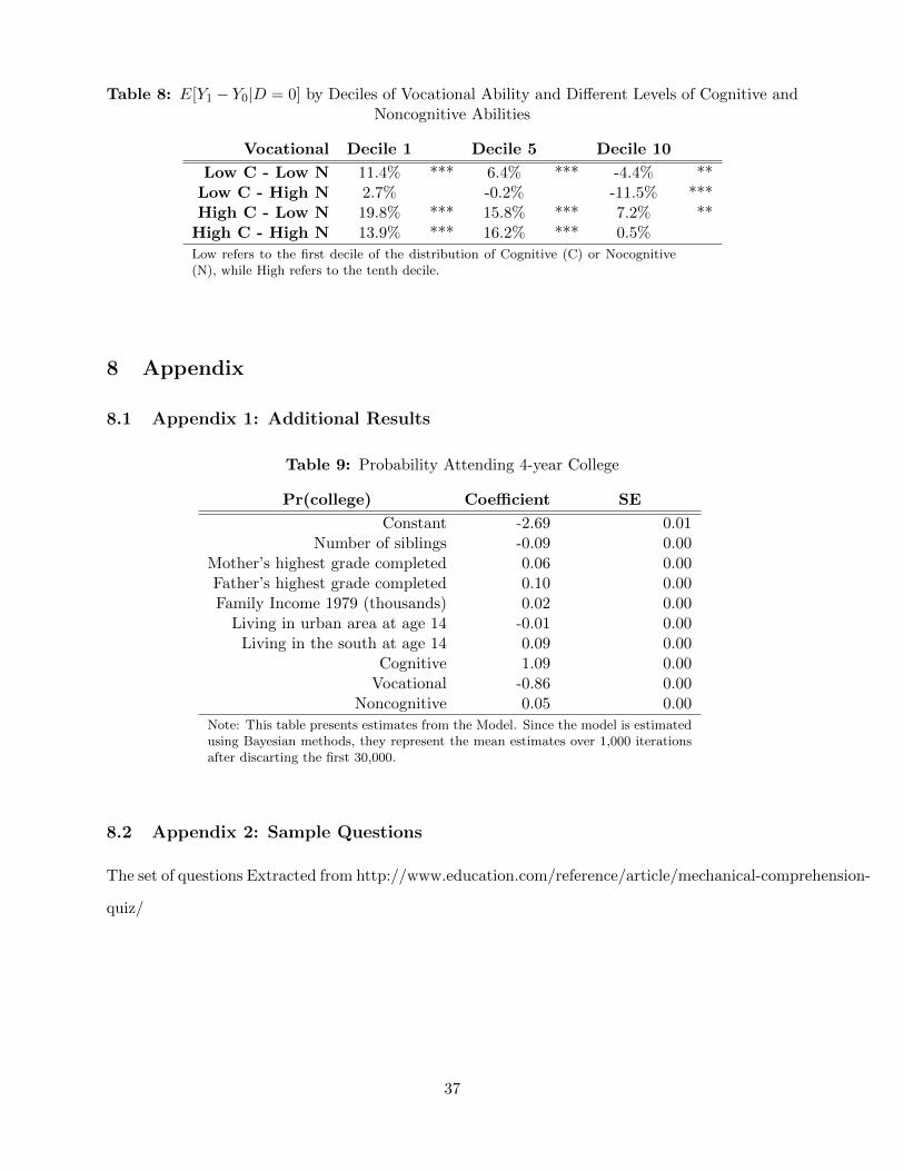
Table 8: E[Y1 − Y0|D = 0] by Deciles of Vocational Ability and Different Levels of Cognitive andNoncognitive Abilities

Vocational Decile 1 Decile 5 Decile 10

Low C - Low N 11.4% *** 6.4% *** -4.4% **Low C - High N 2.7% -0.2% -11.5% ***High C - Low N 19.8% *** 15.8% *** 7.2% **

High C - High N 13.9% *** 16.2% *** 0.5%

Low refers to the first decile of the distribution of Cognitive (C) or Nocognitive(N), while High refers to the tenth decile.

8 Appendix

8.1 Appendix 1: Additional Results

Table 9: Probability Attending 4-year College

Pr(college) Coefficient SE

Constant -2.69 0.01Number of siblings -0.09 0.00

Mother’s highest grade completed 0.06 0.00Father’s highest grade completed 0.10 0.00Family Income 1979 (thousands) 0.02 0.00

Living in urban area at age 14 -0.01 0.00Living in the south at age 14 0.09 0.00

Cognitive 1.09 0.00Vocational -0.86 0.00

Noncognitive 0.05 0.00

Note: This table presents estimates from the Model. Since the model is estimatedusing Bayesian methods, they represent the mean estimates over 1,000 iterationsafter discarting the first 30,000.

8.2 Appendix 2: Sample Questions

The set of questions Extracted from http://www.education.com/reference/article/mechanical-comprehension-

quiz/

37

Table 10: Log Hourly Wages by College Decision

w|D=0 SE w|D=1 SE

Constant 2.98 0.00 2.70 0.00Northeast residence 0.04 0.00 0.34 0.00

Northcentral residence -0.15 0.00 0.11 0.00South residence -0.14 0.00 0.12 0.00

Cohort1 (Born 57-58) -0.04 0.00 0.24 0.00Cohort2 (Born 59-60) -0.06 0.00 0.18 0.00Cohort3 (Born 61-62) -0.09 0.00 0.16 0.00

Local Unemployment rate -0.63 0.02 -1.70 0.02Cognitive 0.05 0.00 0.16 0.00

Vocational 0.10 0.00 -0.03 0.00Noncognitive 0.06 0.00 0.03 0.00

Note: This table presents estimates from the Model. Since the model is estimatedusing Bayesian methods, they represent the mean estimates over 1,000 iterationsafter discarting the first 30,000.

Table 11: Parameters of the Distribution of Unobserved Abilities

Cognitive Vocational NoncognitiveEstimate SE Estimate SE Estimate SE

µ1 0.37 0.13 0.38 0.06 1.05 0.13µ2 -0.65 0.33 -0.39 0.12 -0.54 0.08

1/σ21 3.52 0.91 12.59 2.90 6.01 1.98

1/σ22 2.55 0.99 5.06 1.20 4.11 1.12

p 0.60 0.19 0.50 0.11 0.34 0.061-p 0.40 0.19 0.50 0.11 0.66 0.06

Note: This table presents estimates from the Model. Since the model is estimatedusing Bayesian methods, they represent the mean estimates over 1,000 iterationsafter discarting the first 30,000.

38

8.2.1 Mechanical Comprenhension Section

1. The diagram shows a class 1 lever. Which of the following is the same kind of lever? A. A pair

of tweezers B. A pair of scissors C. A wheelbarrow D. A pair of tongs

2. The diagram shows a class 2 lever. Which of the following is the same kind of lever? A. A

seesaw B. A pair of scissors C. The human forearm D. A wheelbarrow

3. When a mass of air expands, which of the following is most likely to happen? A. The air

warms up. B. The air cools down. C. The air stays at the same temperature. D. The air

contracts.

4. The diagram shows a class 3 lever. Which of the following is the same kind of lever? A. A

pair of tweezers B. A wheelbarrow C. A seesaw D. A wedge

5. Which of the following would feel hottest to the touch if one end were placed in a pot of

boiling water? A. A wooden spoon B. A metal fork C. A plastic knife D. A plastic cup

6. In the diagram, what can you tell about the load on posts A and B? A. Post B carries more

weight. B. Post A carries more weight. C. Post A carries no weight. D. The load is equal on

posts A and B.

7. Water is flowing through this pipe. Which statement is true? A. Water is moving faster at

point A than at point B. Water pressure is equal at points A and B. C. Water pressure is

greater at point A than at point B. D. Water pressure is greater at point B than at point A.

8. What is the advantage of using triangle shapes in constructing a bridge? A. Triangles are

sturdier than other shapes. B. Triangles are very flexible. C. Triangles are inexpensive to

manufacture. D. Triangles are attractive to look at.

39

9. Shifting to a smaller gear on a mountain bike will have an effect on the speed of travel. The

smaller sized gear will make pedaling easier but it will also a. increase the speed of travel. b.

decrease the speed of travel. c. have no effect on the speed of travel. d. make the bicyclist

work harder.

10. Which of the following examples does not make use of a wedge? a. Choosing a sand wedge

to hit your golf ball b. Splitting firewood with a chisel and sledge hammer c. Chopping wood

with an axe d. Using a lever to lift a load

11. A block and tackle refers to a device which is used to a. put under the wheel of a vehicle

to prevent it from rolling backward. b. prevent fish from escaping the hook. c. leverage a

stationary object. d. hoist an object into the air by means of rope and pulleys.

12. Downshifting an auto or a truck causes a. a decrease in speed and an increase in torque. b.

an increase in speed and a decrease in torque. c. no change in speed and no change in torque.

d. None of the above

13. Shifting to a higher gear in a car or truck causes a. a decrease in torque and an increase in

speed. b. an increase in torque and a decrease in speed. c. an increase in both speed and

torque. d. None of the above.

8.2.2 Automotive and Shop Information

1. A car uses too much oil when which of the following parts are worn? A. pistons B. piston

rings C. main bearings D. connecting rods

2. What system of an automobile or truck determines the vehicle’s cornering ability and ride

stiffness? a. Steering system b. Braking system c. Electrical system d. Suspension system

3. The purpose of a transfer case is to a. make a vehicle ride more smoothly. b. make the

steering more responsive to driver input. c. distribute power to front and rear wheels in a 4

x 4 vehicle. d. shorten the braking distance.

4. The reason a particular quarter inch nut may not fit a particular quarter inch bolt is because

a. they may be of different thread classifications. b. a quarter inch bolt is incompatible with

40

a quarter inch nut of the same size. c. the metal alloys from which the nut and bolt are made

may cause the nut to seize.d. quarter-inch bolts require a nut of a slightly larger size to fit.

5. The kerf is a. a type of wood file. b. the angle of the blade on a circular saw. c. a slot or

cut made by the blade of a saw as it cuts into the wood. d. a term of measurement used in

vehicle wheel alignment.

6. It would be better to use thick viscosity motor oil in a. cold climates (makes vehicle startups

easier). b. tropical climates (engine heat build-up). c. Eastern United States. d. four-wheel

drive vehicles.

7. The part of the motor vehicle electric system which distributes the spark to the various

combustion cylinders is the a. battery. b. rotor and distributor assembly. c. injection

system. d. ignition coil.

8. A punch is used for a. hammering knots from wooden objects. b. marking metal or wooden

objects to prepare for drilling or other activities and for driving small headed nails. c. filing

the sharp edges of metal or wooden objects. d. drilling holes.

9. For a better grip on a stubborn fastener nut, it is better to use a. an adjustable wrench. b.

an open-end wrench. c. a box-end wrench. d. a pipe wrench.

8.2.3 Electronics Information

1. Ohm’s Law states that a. E = I x R. b. R = E x I. c. voltage is equal to the current

multiplied by the resistance. d. Both a and c

2. The electrons revolve around the nucleus in a cumulative series of orbits which are called a.

neutrons. b. subatomic particles. c. shells. d. circulating cores.

3. The part of the atom’s shell that determines electrical properties is the shell. a.

insulator b. nucleic c. valence d. electronic

4. A semi-conductor is an element or substance which a. conducts electricity better than a

conductor. b. is useful for certain conductive requirements necessary to some electrical

41

technologies. c. completely inhibits the flow of electrons around the outer shell. d. insulates

electrical current from contact with other materials.

5. When applied to electrical conductivity of household current, 60 hertz means that a. current

flows in only one direction. b. current flows in two directions. c. current flows first in one

direction and then another. d. 60 voltage cycles take place in one second.

6. The three necessary components of an electrical circuit are a. an electrical load, conductors,

and a circuit for the electricity flow to follow. b. a switch, a resistor, and a path to follow. c.

a 60 hertz receptacle, a switch, and a power source. d. a closed circuit, a battery, and radio

waves.

7. Doping is a term used in the semiconductor process when a. impurities are added into the

crystal structure of silicon. b. hydrogen atoms are added to the crystal structure of silicon.

c. impurities are removed from the crystal structure of silicon. d. semiconductors are used

for medical purposes.

8. The property of electricity that pushes and moves it along a circuit is called a. alternating

current. b. amperage. c. resistance. d. voltage.

42

References

Altonji, J. (2010). Multiple skills, multiple types of education, and the labor market: A research

agenda. note AEA: Ten Years and Beyond: Economists Answer NSF’s Call for Long-Term

Research Agendas.

Bishop, J. (1988). Occupational competency as a predictor of labor market performance. Cornell

University, School of Industrial and Labor Relations.

Borghans, L., A. L. Duckworth, J. J. Heckman, and B. ter Weel (2008, Fall). The economics and

psychology of personality traits. Journal of Human Resources 43 (4), 972–1059.

Bowles, S., H. Gintis, and M. Osborne (2001, May). Incentive-enhancing preferences: Personality,

behavior, and earnings. American Economic Review 91 (2), 155–158.

Cameron, S. V. and J. J. Heckman (1998, April). Life cycle schooling and dynamic selection bias:

Models and evidence for five cohorts of American males. Journal of Political Economy 106 (2),

262–333.

Cameron, S. V. and J. J. Heckman (2001, June). The dynamics of educational attainment for

black, hispanic, and white males. Journal of Political Economy 109 (3), 455–99.

Carneiro, P., K. Hansen, and J. J. Heckman (2003, May). Estimating distributions of treatment ef-

fects with an application to the returns to schooling and measurement of the effects of uncertainty

on college choice. International Economic Review 44 (2), 361–422.

Cawley, J., J. J. Heckman, and E. J. Vytlacil (2001, September). Three observations on wages and

measured cognitive ability. Labour Economics 8 (4), 419–442.

Dickens, W. T. (2008). Cognitive Ability. The New Palgrave Dictionary of Economics. Steve Durlauf

ed.

Diekhoff, G. (1992). Statistics for the social and behavioral sciences: Univariate, bivariate, multi-

variate. Wm. C. Brown Publishers (Dubuque, IA).

43

Ellwood, D. T. and T. J. Kane (2000). Who is getting a college education? Family background and

the growing gaps in enrollment. In S. Danziger and J. Waldfogel (Eds.), Securing the Future:

Investing in Children from Birth to College, pp. 283–324. New York: Russell Sage Foundation.

Farkas, G. (2003, August). Cognitive skills and noncognitive traits and behaviors in stratification

processes. Annual Review of Sociology 29, 541–562.

Ferguson, T. S. (1983). Bayesian density estimation by mixtures of normal distributions. In

H. Chernoff, M. Rizvi, J. Rustagi, and D. Siegmund (Eds.), Recent Advances in Statistics: Papers

in Honor of Herman Chernoff on his Sixtieth Birthday, pp. 287–302. New York: Academic Press.

Hansen, K. T., J. J. Heckman, and K. J. Mullen (2004, July–August). The effect of schooling and

ability on achievement test scores. Journal of Econometrics 121 (1-2), 39–98.

Heckman, J. J. (1995). Notes on schooling, earnings and ability. Unpublished manuscript, Univer-

sity of Chicago, Department of Economics.

Heckman, J. J., J. Stixrud, and S. Urzua (2006, July). The effects of cognitive and noncognitive

abilities on labor market outcomes and social behavior. Journal of Labor Economics 24 (3),

411–482.

Herrnstein, R. J. and C. A. Murray (1994). The Bell Curve: Intelligence and Class Structure in

American Life. New York: Free Press.

Menaghan, E. G. (1990). The impact of occupational and economic pressures on young moth-

ers’ self-esteem: Evidence from the nlsy. Presented: Annual Meetings of the Society for the

Sociological Study of Social Problems, Washington, D.C., August 9.

Neal, D. A. and W. R. Johnson (1996, October). The role of premarket factors in black-white wage

differences. Journal of Political Economy 104 (5), 869–895.

O’Neill, J. (1990). The role of human capital in earnings differences between black and white men.

The Journal of Economic Perspectives 4 (4), 25–45.

Osborne-Groves, M. (2004, March). How important is your personality? Labor market returns

to personality for women in the US and UK. Unpublished manuscript, Towson University,

Department of Economics. In press at Journal of Economic Psychology.

44

Rosenberg, M. (1965). Society and the Adolescent Self-Image. Princeton, NJ: Princeton University

Press.

Rotter, J. B. (1966). Generalized Expectancies for Internal versus External Control of Reinforce-

ment. Washington DC: American Psychological Association.

Sheskin, D. (2004). Handbook of Parametric and Nonparametric Statistical Procedures (Third

Edition ed.). Chapman and Hall/CRC Press.

Strocchia-Rivera, L. (1988). Self-Esteem and Educational Aspirations as Antecedents of Adolescent

Unmarried Motherhood. Ph. D. thesis, The University of Texas at Austin.

Urzua, S. (2008, Fall). Racial labor market gaps: The role of abilities and schooling choices. Journal

of Human Resources 43 (4), 919–971.

Willis, R. J. and S. Rosen (1979, October). Education and self-selection. Journal of Political

Economy 87 (5, Part 2), S7–S36.

45