(online only mark schervish -...

INSTRUCTOR’S SOLUTIONS MANUAL

(ONLINE ONLY)

MARK SCHERVISH Carnegie Mellon University

PROBABILITY AND STATISTICS FOURTH EDITION

Morris DeGroot Carnegie Mellon University

Mark Schervish Carnegie Mellon University

Full file at http://TestbankCollege.eu/Solution-Manual-Probability-and-Statistics-4th-Edition-DeGroot

The author and publisher of this book have used their best efforts in preparing this book. These efforts include the development, research, and testing of the theories and programs to determine their effectiveness. The author and publisher make no warranty of any kind, expressed or implied, with regard to these programs or the documentation contained in this book. The author and publisher shall not be liable in any event for incidental or consequential damages in connection with, or arising out of, the furnishing, performance, or use of these programs. Reproduced by Pearson Addison-Wesley from electronic files supplied by the author. Copyright © 2012, 2002, 1986 Pearson Education, Inc. Publishing as Pearson Addison-Wesley, 75 Arlington Street, Boston, MA 02116. All rights reserved. This manual may be reproduced for classroom use only. ISBN-13: 978-0-321-71597-5 ISBN-10: 0-321-71597-7

Full file at http://TestbankCollege.eu/Solution-Manual-Probability-and-Statistics-4th-Edition-DeGroot

http://TestbankCollege.eu/Solution-Manual-Probability-and-Statistics-4th-Edition-DeGroot

Contents

Preface . . . . . . . . . . . . . . . . . . . . . . . . . . . . . . . . . . . . . . . . . . . . . . . . . . . vi

1 Introduction to Probability 1

1.2 Interpretations of Probability . . . . . . . . . . . . . . . . . . . . . . . . . . . . . . . . . . . . 1

1.4 Set Theory . . . . . . . . . . . . . . . . . . . . . . . . . . . . . . . . . . . . . . . . . . . . . . 1

1.5 The Definition of Probability . . . . . . . . . . . . . . . . . . . . . . . . . . . . . . . . . . . . 3

1.6 Finite Sample Spaces . . . . . . . . . . . . . . . . . . . . . . . . . . . . . . . . . . . . . . . . . 6

1.7 Counting Methods . . . . . . . . . . . . . . . . . . . . . . . . . . . . . . . . . . . . . . . . . . 7

1.8 Combinatorial Methods . . . . . . . . . . . . . . . . . . . . . . . . . . . . . . . . . . . . . . . 8

1.9 Multinomial Coefficients . . . . . . . . . . . . . . . . . . . . . . . . . . . . . . . . . . . . . . . 13

1.10 The Probability of a Union of Events . . . . . . . . . . . . . . . . . . . . . . . . . . . . . . . . 16

1.12 Supplementary Exercises . . . . . . . . . . . . . . . . . . . . . . . . . . . . . . . . . . . . . . . 20

2 Conditional Probability 25

2.1 The Definition of Conditional Probability . . . . . . . . . . . . . . . . . . . . . . . . . . . . . 25

2.2 Independent Events . . . . . . . . . . . . . . . . . . . . . . . . . . . . . . . . . . . . . . . . . 28

2.3 Bayes’ Theorem . . . . . . . . . . . . . . . . . . . . . . . . . . . . . . . . . . . . . . . . . . . . 34

2.4 The Gambler’s Ruin Problem . . . . . . . . . . . . . . . . . . . . . . . . . . . . . . . . . . . . 40


3 Random Variables and Distributions 49

3.1 Random Variables and Discrete Distributions . . . . . . . . . . . . . . . . . . . . . . . . . . . 49

3.2 Continuous Distributions . . . . . . . . . . . . . . . . . . . . . . . . . . . . . . . . . . . . . . 50

3.3 The Cumulative Distribution Function . . . . . . . . . . . . . . . . . . . . . . . . . . . . . . . 53

3.4 Bivariate Distributions . . . . . . . . . . . . . . . . . . . . . . . . . . . . . . . . . . . . . . . . 58

3.5 Marginal Distributions . . . . . . . . . . . . . . . . . . . . . . . . . . . . . . . . . . . . . . . . 64

3.6 Conditional Distributions . . . . . . . . . . . . . . . . . . . . . . . . . . . . . . . . . . . . . . 70

3.7 Multivariate Distributions . . . . . . . . . . . . . . . . . . . . . . . . . . . . . . . . . . . . . . 76

3.8 Functions of a Random Variable . . . . . . . . . . . . . . . . . . . . . . . . . . . . . . . . . . 81

3.9 Functions of Two or More Random Variables . . . . . . . . . . . . . . . . . . . . . . . . . . . 85

3.10 Markov Chains . . . . . . . . . . . . . . . . . . . . . . . . . . . . . . . . . . . . . . . . . . . . 93


4 Expectation 107

4.1 The Expectation of a Random Variable . . . . . . . . . . . . . . . . . . . . . . . . . . . . . . 107

4.2 Properties of Expectations . . . . . . . . . . . . . . . . . . . . . . . . . . . . . . . . . . . . . . 110

4.3 Variance . . . . . . . . . . . . . . . . . . . . . . . . . . . . . . . . . . . . . . . . . . . . . . . . 113

4.4 Moments . . . . . . . . . . . . . . . . . . . . . . . . . . . . . . . . . . . . . . . . . . . . . . . 115

4.5 The Mean and the Median . . . . . . . . . . . . . . . . . . . . . . . . . . . . . . . . . . . . . . 118

Copyright © 2012 Pearson Education, Inc. Publishing as Addison-Wesley.Full file at http://TestbankCollege.eu/Solution-Manual-Probability-and-Statistics-4th-Edition-DeGroot


iv CONTENTS

4.6 Covariance and Correlation . . . . . . . . . . . . . . . . . . . . . . . . . . . . . . . . . . . . . 121

4.7 Conditional Expectation . . . . . . . . . . . . . . . . . . . . . . . . . . . . . . . . . . . . . . . 124

4.8 Utility . . . . . . . . . . . . . . . . . . . . . . . . . . . . . . . . . . . . . . . . . . . . . . . . . 129


5 Special Distributions 141

5.2 The Bernoulli and Binomial Distributions . . . . . . . . . . . . . . . . . . . . . . . . . . . . . 141

5.3 The Hypergeometric Distributions . . . . . . . . . . . . . . . . . . . . . . . . . . . . . . . . . 145

5.4 The Poisson Distributions . . . . . . . . . . . . . . . . . . . . . . . . . . . . . . . . . . . . . . 149

5.5 The Negative Binomial Distributions . . . . . . . . . . . . . . . . . . . . . . . . . . . . . . . . 155

5.6 The Normal Distributions . . . . . . . . . . . . . . . . . . . . . . . . . . . . . . . . . . . . . . 159

5.7 The Gamma Distributions . . . . . . . . . . . . . . . . . . . . . . . . . . . . . . . . . . . . . . 165

5.8 The Beta Distributions . . . . . . . . . . . . . . . . . . . . . . . . . . . . . . . . . . . . . . . . 171

5.9 The Multinomial Distributions . . . . . . . . . . . . . . . . . . . . . . . . . . . . . . . . . . . 174

5.10 The Bivariate Normal Distributions . . . . . . . . . . . . . . . . . . . . . . . . . . . . . . . . 177


6 Large Random Samples 187

6.1 Introduction . . . . . . . . . . . . . . . . . . . . . . . . . . . . . . . . . . . . . . . . . . . . . . 187

6.2 The Law of Large Numbers . . . . . . . . . . . . . . . . . . . . . . . . . . . . . . . . . . . . . 188

6.3 The Central Limit Theorem . . . . . . . . . . . . . . . . . . . . . . . . . . . . . . . . . . . . . 194

6.4 The Correction for Continuity . . . . . . . . . . . . . . . . . . . . . . . . . . . . . . . . . . . . 198


7 Estimation 203

7.1 Statistical Inference . . . . . . . . . . . . . . . . . . . . . . . . . . . . . . . . . . . . . . . . . 203

7.2 Prior and Posterior Distributions . . . . . . . . . . . . . . . . . . . . . . . . . . . . . . . . . . 204

7.3 Conjugate Prior Distributions . . . . . . . . . . . . . . . . . . . . . . . . . . . . . . . . . . . . 207

7.4 Bayes Estimators . . . . . . . . . . . . . . . . . . . . . . . . . . . . . . . . . . . . . . . . . . . 214

7.5 Maximum Likelihood Estimators . . . . . . . . . . . . . . . . . . . . . . . . . . . . . . . . . . 217

7.6 Properties of Maximum Likelihood Estimators . . . . . . . . . . . . . . . . . . . . . . . . . . 220

7.7 Sufficient Statistics . . . . . . . . . . . . . . . . . . . . . . . . . . . . . . . . . . . . . . . . . . 225

7.8 Jointly Sufficient Statistics . . . . . . . . . . . . . . . . . . . . . . . . . . . . . . . . . . . . . . 228

7.9 Improving an Estimator . . . . . . . . . . . . . . . . . . . . . . . . . . . . . . . . . . . . . . . 230


8 Sampling Distributions of Estimators 239

8.1 The Sampling Distribution of a Statistic . . . . . . . . . . . . . . . . . . . . . . . . . . . . . . 239

8.2 The Chi-Square Distributions . . . . . . . . . . . . . . . . . . . . . . . . . . . . . . . . . . . . 241

8.3 Joint Distribution of the Sample Mean and Sample Variance . . . . . . . . . . . . . . . . . . 245

8.4 The t Distributions . . . . . . . . . . . . . . . . . . . . . . . . . . . . . . . . . . . . . . . . . . 247

8.5 Confidence Intervals . . . . . . . . . . . . . . . . . . . . . . . . . . . . . . . . . . . . . . . . . 250

8.6 Bayesian Analysis of Samples from a Normal Distribution . . . . . . . . . . . . . . . . . . . . 254

8.7 Unbiased Estimators . . . . . . . . . . . . . . . . . . . . . . . . . . . . . . . . . . . . . . . . . 258

8.8 Fisher Information . . . . . . . . . . . . . . . . . . . . . . . . . . . . . . . . . . . . . . . . . . 263




CONTENTS v

9 Testing Hypotheses 273

9.1 Problems of Testing Hypotheses . . . . . . . . . . . . . . . . . . . . . . . . . . . . . . . . . . . 2739.2 Testing Simple Hypotheses . . . . . . . . . . . . . . . . . . . . . . . . . . . . . . . . . . . . . 2789.3 Uniformly Most Powerful Tests . . . . . . . . . . . . . . . . . . . . . . . . . . . . . . . . . . . 2849.4 Two-Sided Alternatives . . . . . . . . . . . . . . . . . . . . . . . . . . . . . . . . . . . . . . . 2899.5 The t Test . . . . . . . . . . . . . . . . . . . . . . . . . . . . . . . . . . . . . . . . . . . . . . . 2939.6 Comparing the Means of Two Normal Distributions . . . . . . . . . . . . . . . . . . . . . . . 2969.7 The F Distributions . . . . . . . . . . . . . . . . . . . . . . . . . . . . . . . . . . . . . . . . . 2999.8 Bayes Test Procedures . . . . . . . . . . . . . . . . . . . . . . . . . . . . . . . . . . . . . . . . 3039.9 Foundational Issues . . . . . . . . . . . . . . . . . . . . . . . . . . . . . . . . . . . . . . . . . . 3079.10 Supplementary Exercises . . . . . . . . . . . . . . . . . . . . . . . . . . . . . . . . . . . . . . . 309

10 Categorical Data and Nonparametric Methods 315

10.1 Tests of Goodness-of-Fit . . . . . . . . . . . . . . . . . . . . . . . . . . . . . . . . . . . . . . . 31510.2 Goodness-of-Fit for Composite Hypotheses . . . . . . . . . . . . . . . . . . . . . . . . . . . . 31710.3 Contingency Tables . . . . . . . . . . . . . . . . . . . . . . . . . . . . . . . . . . . . . . . . . . 32010.4 Tests of Homogeneity . . . . . . . . . . . . . . . . . . . . . . . . . . . . . . . . . . . . . . . . 32310.5 Simpson’s Paradox . . . . . . . . . . . . . . . . . . . . . . . . . . . . . . . . . . . . . . . . . . 32510.6 Kolmogorov-Smirnov Tests . . . . . . . . . . . . . . . . . . . . . . . . . . . . . . . . . . . . . 32710.7 Robust Estimation . . . . . . . . . . . . . . . . . . . . . . . . . . . . . . . . . . . . . . . . . . 33310.8 Sign and Rank Tests . . . . . . . . . . . . . . . . . . . . . . . . . . . . . . . . . . . . . . . . . 33710.9 Supplementary Exercises . . . . . . . . . . . . . . . . . . . . . . . . . . . . . . . . . . . . . . . 342

11 Linear Statistical Models 349

11.1 The Method of Least Squares . . . . . . . . . . . . . . . . . . . . . . . . . . . . . . . . . . . . 34911.2 Regression . . . . . . . . . . . . . . . . . . . . . . . . . . . . . . . . . . . . . . . . . . . . . . . 35311.3 Statistical Inference in Simple Linear Regression . . . . . . . . . . . . . . . . . . . . . . . . . 35611.4 Bayesian Inference in Simple Linear Regression . . . . . . . . . . . . . . . . . . . . . . . . . . 36411.5 The General Linear Model and Multiple Regression . . . . . . . . . . . . . . . . . . . . . . . . 36611.6 Analysis of Variance . . . . . . . . . . . . . . . . . . . . . . . . . . . . . . . . . . . . . . . . . 37311.7 The Two-Way Layout . . . . . . . . . . . . . . . . . . . . . . . . . . . . . . . . . . . . . . . . 37811.8 The Two-Way Layout with Replications . . . . . . . . . . . . . . . . . . . . . . . . . . . . . . 38311.9 Supplementary Exercises . . . . . . . . . . . . . . . . . . . . . . . . . . . . . . . . . . . . . . . 389

12 Simulation 399

12.1 What is Simulation? . . . . . . . . . . . . . . . . . . . . . . . . . . . . . . . . . . . . . . . . . 40012.2 Why Is Simulation Useful? . . . . . . . . . . . . . . . . . . . . . . . . . . . . . . . . . . . . . . 40012.3 Simulating Specific Distributions . . . . . . . . . . . . . . . . . . . . . . . . . . . . . . . . . . 40412.4 Importance Sampling . . . . . . . . . . . . . . . . . . . . . . . . . . . . . . . . . . . . . . . . . 41012.5 Markov Chain Monte Carlo . . . . . . . . . . . . . . . . . . . . . . . . . . . . . . . . . . . . . 41412.6 The Bootstrap . . . . . . . . . . . . . . . . . . . . . . . . . . . . . . . . . . . . . . . . . . . . 42112.7 Supplementary Exercises . . . . . . . . . . . . . . . . . . . . . . . . . . . . . . . . . . . . . . . 425R Code For Two Text Examples . . . . . . . . . . . . . . . . . . . . . . . . . . . . . . . . . . . . . 432



vi CONTENTS

Preface

This manual contains solutions to all of the exercises in Probability and Statistics, 4th edition, by MorrisDeGroot and myself. I have preserved most of the solutions to the exercises that existed in the 3rd edition.Certainly errors have been introduced, and I will post any errors brought to my attention on my web pagehttp://www.stat.cmu.edu/ mark/ along with errors in the text itself. Feel free to send me comments.

For instructors who are familiar with earlier editions, I hope that you will find the 4th edition at least asuseful. Some new material has been added, and little has been removed. Assuming that you will be spendingthe same amount of time using the text as before, something will have to be skipped. I have tried to arrangethe material so that instructors can choose what to cover and what not to cover based on the type of coursethey want. This manual contains commentary on specific sections right before the solutions for those sections.This commentary is intended to explain special features of those sections and help instructors decide whichparts they want to require of their students. Special attention is given to more challenging material and howthe remainder of the text does or does not depend upon it.

To teach a mathematical statistics course for students with a strong calculus background, one could safelycover all of the material for which one could find time. The Bayesian sections include 4.8, 7.2, 7.3, 7.4, 8.6,9.8, and 11.4. One can choose to skip some or all of this material if one desires, but that would be ignoringone of the unique features of the text. The more challenging material in Sections 7.7–7.9, and 9.2–9.4 is reallyonly suitable for a mathematical statistics course. One should try to make time for some of the material inSections 12.1–12.3 even if it meant cutting back on some of the nonparametrics and two-way ANOVA. To teacha more modern statistics course, one could skip Sections 7.7–7.9, 9.2–9.4, 10.8, and 11.7–11.8. This wouldleave time to discuss robust estimation (Section 10.7) and simulation (Chapter 12). Section 3.10 on Markovchains is not actually necessary even if one wishes to introduce Markov chain Monte Carlo (Section 12.5),although it is helpful for understanding what this topic is about.

Using Statistical Software

The text was written without reference to any particular statistical or mathematical software. However,there are several places throughout the text where references are made to what general statistical softwaremight be able to do. This is done for at least two reasons. One is that different instructors who wish to usestatistical software while teaching will generally choose different programs. I didn’t want the text to be tiedto a particular program to the exclusion of others. A second reason is that there are still many instructorsof mathematical probability and statistics courses who prefer not to use any software at all.

Given how pervasive computing is becoming in the use of statistics, the second reason above is becomingless compelling. Given the free and multiplatform availability and the versatility of the environment R, eventhe first reason is becoming less compelling. Throughout this manual, I have inserted pointers to which R

functions will perform many of the calculations that would formerly have been done by hand when using thistext. The software can be downloaded for Unix, Windows, or Mac OS fromhttp://www.r-project.org/

That site also has manuals for installation and use. Help is also available directly from within the R envi-ronment.

Many tutorials for getting started with R are available online. At the official R site there is the detailedmanual: http://cran.r-project.org/doc/manuals/R-intro.htmlthat starts simple and has a good table of contents and lots of examples. However, reading it from start tofinish is not an efficient way to get started. The sample sessions should be most helpful.

One major issue with using an environment like R is that it is essentially programming. That is, studentswho have never programmed seriously before are going to have a steep learning curve. Without going intothe philosophy of whether students should learn statistics without programming, the field is moving in thedirection of requiring programming skills. People who want only to understand what a statistical analysis



CONTENTS vii

is about can still learn that without being able to program. But anyone who actually wants to do statisticsas part of their job will be seriously handicapped without programming ability. At the end of this manualis a series of heavily commented R programms that illustrate many of the features of R in the context of aspecific example from the text.

Mark J. Schervish



Chapter 1

Introduction to Probability

1.2 Interpretations of Probability

Commentary

It is interesting to have the students determine some of their own subjective probabilities. For example, letX denote the temperature at noon tomorrow outside the building in which the class is being held. Have eachstudent determine a number x1 such that the student considers the following two possible outcomes to beequally likely: X ≤ x1 andX > x1. Also, have each student determine numbers x2 and x3 (with x2 < x3) suchthat the student considers the following three possible outcomes to be equally likely: X ≤ x2, x2 < X < x3,and X ≥ x3. Determinations of more than three outcomes that are considered to be equally likely can alsobe made. The different values of x1 determined by different members of the class should be discussed, andalso the possibility of getting the class to agree on a common value of x1.

Similar determinations of equally likely outcomes can be made by the students in the class for quantitiessuch as the following ones which were found in the 1973 World Almanac and Book of Facts: the numberof freight cars that were in use by American railways in 1960 (1,690,396), the number of banks in theUnited States which closed temporarily or permanently in 1931 on account of financial difficulties (2,294),and the total number of telephones which were in service in South America in 1971 (6,137,000).

1.4 Set Theory

Solutions to Exercises

1. Assume that x ∈ Bc. We need to show that x ∈ Ac. We shall show this indirectly. Assume, to thecontrary, that x ∈ A. Then x ∈ B because A ⊂ B. This contradicts x ∈ Bc. Hence x ∈ A is false andx ∈ Ac.

2. First, show that A ∩ (B ∪ C) ⊂ (A ∩B) ∪ (A ∩ C). Let x ∈ A ∩ (B ∪ C). Then x ∈ A and x ∈ B ∪ C.That is, x ∈ A and either x ∈ B or x ∈ C (or both). So either (x ∈ A and x ∈ B) or (x ∈ Aand x ∈ C) or both. That is, either x ∈ A ∩ B or x ∈ A ∩ C. This is what it means to say thatx ∈ (A∩B)∪ (A∩C). Thus A∩ (B∪C) ⊂ (A∩B)∪ (A∩C). Basically, running these steps backwardsshows that (A ∩B) ∪ (A ∩C) ⊂ A ∩ (B ∪C).

3. To prove the first result, let x ∈ (A ∪ B)c. This means that x is not in A ∪ B. In other words, x isneither in A nor in B. Hence x ∈ Ac and x ∈ Bc. So x ∈ Ac∩Bc. This proves that (A∪B)c ⊂ Ac∩Bc.Next, suppose that x ∈ Ac ∩Bc. Then x ∈ Ac and x ∈ Bc. So x is neither in A nor in B, so it can’t bein A ∪ B. Hence x ∈ (A ∪ B)c. This shows that Ac ∩ Bc ⊂ (A ∪ B)c. The second result follows fromthe first by applying the first result to Ac and Bc and then taking complements of both sides.



2 Chapter 1. Introduction to Probability

4. To see that A∩B and A∩Bc are disjoint, let x ∈ A∩B. Then x ∈ B, hence x �∈ Bc and so x �∈ A∩Bc. Sono element of A∩B is in A∩Bc, hence the two events are disjoint. To prove that A = (A∩B)∪(A∩Bc),we shall show that each side is a subset of the other side. First, let x ∈ A. Either x ∈ B or x ∈ Bc. Ifx ∈ B, then x ∈ A ∩ B. If x ∈ Bc, then x ∈ A ∩ Bc. Either way, x ∈ (A ∩ B) ∪ (A ∩ Bc). So everyelement of A is an element of (A∩B)∪ (A∩Bc) and we conclude that A ⊂ (A∩B)∪ (A∩Bc). Finally,let x ∈ (A ∩ B) ∪ (A ∩ Bc). Then either x ∈ A ∩ B, in which case x ∈ A, or x ∈ A ∩ Bc, in whichcase x ∈ A. Either way x ∈ A, so every element of (A ∩ B) ∪ (A ∩ Bc) is also an element of A and(A ∩B) ∪ (A ∩Bc) ⊂ A.

5. To prove the first result, let x ∈ (∪iAi)c. This means that x is not in ∪iAi. In other words, for every

i ∈ I, x is not in Ai. Hence for every i ∈ I, x ∈ Aci . So x ∈ ∩iA

ci . This proves that (∪iAi)

c ⊂ ∩iAci .

Next, suppose that x ∈ ∩iAci . Then x ∈ Ac

i for every i ∈ I. So for every i ∈ I, x is not in Ai. So xcan’t be in ∪iAi. Hence x ∈ (∪iAi)

c. This shows that ∩iAci ⊂ (∪iAi)

c. The second result follows fromthe first by applying the first result to Ac

i for i ∈ I and then taking complements of both sides.

6. (a) Blue card numbered 2 or 4.

(b) Blue card numbered 5, 6, 7, 8, 9, or 10.

(c) Any blue card or a red card numbered 1, 2, 3, 4, 6, 8, or 10.

(d) Blue card numbered 2, 4, 6, 8, or 10, or red card numbered 2 or 4.

(e) Red card numbered 5, 7, or 9.

7. (a) These are the points not in A, hence they must be either below 1 or above 5. That is Ac = {x :x < 1 or x > 5}.

(b) These are the points in either A or B or both. So they must be between 1 and 5 or between 3 and7. That is, A ∪B = {x : 1 ≤ x ≤ 7}.

(c) These are the points in B but not in C. That is BCc = {x : 3 < x ≤ 7}. (Note that B ⊂ Cc.)

(d) These are the points in none of the three sets, namely AcBcCc = {x : 0 < x < 1 or x > 7}.(e) These are the points in the answer to part (b) and in C. There are no such values and (A∪B)C = ∅.

8. Blood type A reacts only with anti-A, so type A blood corresponds to A ∩ Bc. Type B blood reactsonly with anti-B, so type B blood corresponds to AcB. Type AB blood reacts with both, so A ∩ Bcharacterizes type AB blood. Finally, type O reacts with neither antigen, so type O blood correspondsto the event AcBc.

9. (a) For each n, Bn = Bn+1 ∪ An, hence Bn ⊃ Bn+1 for all n. For each n, Cn+1 ∩ An = Cn, soCn ⊂ Cn+1.

(b) Suppose that x ∈ ∩∞n=1Bn. Then x ∈ Bn for all n. That is, x ∈ ∪∞

i=nAi for all n. For n = 1, thereexists i ≥ n such that x ∈ Ai. Assume to the contrary that there are at most finitely many i suchthat x ∈ Ai. Let m be the largest such i. For n = m+ 1, we know that there is i ≥ n such thatx ∈ Ai. This contradicts m being the largest i such that x ∈ Ai. Hence, x is in infinitely manyAi. For the other direction, assume that x is in infinitely many Ai. Then, for every n, there is avalue of j > n such that x ∈ Aj , hence x ∈ ∪∞

i=nAi = Bn for every n and x ∈ ∩∞n=1Bn.

(c) Suppose that x ∈ ∪∞n=1Cn. That is, there exists n such that x ∈ Cn = ∩∞

i=nAi, so x ∈ Ai forall i ≥ n. So, there at most finitely many i (a subset of 1, . . . , n − 1) such that x �∈ Ai. Finally,suppose that x ∈ Ai for all but finitely many i. Let k be the last i such that x �∈ Ai. Then x ∈ Ai

for all i ≥ k + 1, hence x ∈ ∩∞i=k+1Ai = Ck+1. Hence x ∈ ∪∞

n=1Cn.



Section 1.5. The Definition of Probability 3

10. (a) All three dice show even numbers if and only if all three of A, B, and C occur. So, the event isA ∩B ∩ C.

(b) None of the three dice show even numbers if and only if all three of Ac, Bc, and Cc occur. So, theevent is Ac ∩Bc ∩ Cc.

(c) At least one die shows an odd number if and only if at least one of Ac, Bc, and Cc occur. So, theevent is Ac ∪Bc ∪ Cc.

(d) At most two dice show odd numbers if and only if at least one die shows an even number, sothe event is A ∪ B ∪ C. This can also be expressed as the union of the three events of the formA∩B∩Cc where exactly one die shows odd together with the three events of the form A∩Bc∩Cc

where exactly two dice show odd together with the even A ∩B ∩ C where no dice show odd.

(e) We can enumerate all the sums that are no greater than 5: 1+1+1, 2+1+1, 1+2+1, 1+1+2,2 + 2 + 1, 2 + 1 + 2, and 1 + 2 + 2. The first of these corresponds to the event A1 ∩B1 ∩ C1, thesecond to A2 ∩B1 ∩ C1, etc. The union of the seven such events is what is requested, namely

(A1∩B1∩C1)∪(A2∩B1∩C1)∪(A1∩B2∩C1)∪(A1∩B1∩C2)∪(A2∩B2∩C1)∪(A2∩B1∩C2)∪(A1∩B2∩C2).

11. (a) All of the events mentioned can be determined by knowing the voltages of the two subcells. Hencethe following set can serve as a sample space

S = {(x, y) : 0 ≤ x ≤ 5 and 0 ≤ y ≤ 5},where the first coordinate is the voltage of the first subcell and the second coordinate is the voltageof the second subcell. Any more complicated set from which these two voltages can be determinedcould serve as the sample space, so long as each outcome could at least hypothetically be learned.

(b) The power cell is functional if and only if the sum of the voltages is at least 6. Hence, A = {(x, y) ∈S : x + y ≥ 6}. It is clear that B = {(x, y) ∈ S : x = y} and C = {(x, y) ∈ S : x > y}. Thepowercell is not functional if and only if the sum of the voltages is less than 6. It needs less thanone volt to be functional if and only if the sum of the voltages is greater than 5. The intersectionof these two is the event D = {(x, y) ∈ S : 5 < x + y < 6}. The restriction “∈ S” that appearsin each of these descriptions guarantees that the set is a subset of S. One could leave off thisrestriction and add the two restrictions 0 ≤ x ≤ 5 and 0 ≤ y ≤ 5 to each set.

(c) The description can be worded as “the power cell is not functional, and needs at least one morevolt to be functional, and both subcells have the same voltage.” This is the intersection of Ac, Dc,and B. That is, Ac ∩Dc ∩B. The part of Dc in which x+ y ≥ 6 is not part of this set because ofthe intersection with Ac.

(d) We need the intersection of Ac (not functional) with Cc (second subcell at least as big as first) andwith Bc (subcells are not the same). In particular, Cc ∩Bc is the event that the second subcell isstrictly higher than the first. So, the event is Ac ∩Bc ∩ Cc.

1.5 The Definition of Probability


1. Define the following events:

A = {the selected ball is red},B = {the selected ball is white},C = {the selected ball is either blue, yellow, or green}.




We are asked to find Pr(C). The three events A, B, and C are disjoint and A ∪ B ∪ C = S. So1 = Pr(A) + Pr(B) + Pr(C). We are told that Pr(A) = 1/5 and Pr(B) = 2/5. It follows thatPr(C) = 2/5.

2. Let B be the event that a boy is selected, and let G be the event that a girl is selected. We are toldthat B ∪G = S, so G = Bc. Since Pr(B) = 0.3, it follows that Pr(G) = 0.7.

3. (a) If A and B are disjoint then B ⊂ Ac and BAc = B, so Pr(BAc) = Pr(B) = 1/2.

(b) If A ⊂ B, then B = A ∪ (BAc) with A and BAc disjoint. So Pr(B) = Pr(A) + Pr(BAc). That is,1/2 = 1/3 + Pr(BAc), so Pr(BAc) = 1/6.

(c) According to Theorem 1.4.11, B = (BA) ∪ (BAc). Also, BA and BAc are disjoint so, Pr(B) =Pr(BA) + Pr(BAc). That is, 1/2 = 1/8 + Pr(BAc), so Pr(BAc) = 3/8.

4. Let E1 be the event that student A fails and let E2 be the event that student B fails. We wantPr(E1 ∪ E2). We are told that Pr(E1) = 0.5, Pr(E2) = 0.2, and Pr(E1E2) = 0.1. According toTheorem 1.5.7, Pr(E1 ∪ E2) = 0.5 + 0.2− 0.1 = 0.6.

5. Using the same notation as in Exercise 4, we now want Pr(Ec1 ∩ Ec

2). According to Theorems 1.4.9and 1.5.3, this equals 1− Pr(E1 ∪E2) = 0.4.

6. Using the same notation as in Exercise 4, we now want Pr([E1 ∩Ec2]∪ [Ec

1 ∩E2]). These two events aredisjoint, so

Pr([E1 ∩ Ec2] ∪ [Ec

1 ∩ E2]) = Pr(E1 ∩ Ec2) + Pr(Ec

1 ∩ E2).

Use the reasoning from part (c) of Exercise 3 above to conclude that

Pr(E1 ∩ Ec2) = Pr(E1)− Pr(E1 ∩E2) = 0.4,

Pr(Ec1 ∩E2) = Pr(E2)− Pr(E1 ∩E2) = 0.1.

It follows that the probability we want is 0.5.

7. Rearranging terms in Eq. (1.5.1) of the text, we get

Pr(A ∩B) = Pr(A) + Pr(B)− Pr(A ∪B) = 0.4 + 0.7 − Pr(A ∪B) = 1.1− Pr(A ∪B).

So Pr(A ∩ B) is largest when Pr(A ∪ B) is smallest and vice-versa. The smallest possible value forPr(A∪B) occurs when one of the events is a subset of the other. In the present exercise this could onlyhappen if A ⊂ B, in which case Pr(A ∪B) = Pr(B) = 0.7, and Pr(A ∩ B) = 0.4. The largest possiblevalue of Pr(A ∪ B) occurs when either A and B are disjoint or when A ∪ B = S. The former is notpossible since the probabilities are too large, but the latter is possible. In this case Pr(A ∪B) = 1 andPr(A ∩B) = 0.1.

8. Let A be the event that a randomly selected family subscribes to the morning paper, and let B be theevent that a randomly selected family subscribes to the afternoon paper. We are told that Pr(A) = 0.5,Pr(B) = 0.65, and Pr(A∪B) = 0.85. We are asked to find Pr(A∩B). Using Theorem 1.5.7 in the textwe obtain

Pr(A ∩B) = Pr(A) + Pr(B)− Pr(A ∪B) = 0.5 + 0.65 − 0.85 = 0.3.



Section 1.5. The Definition of Probability 5

9. The required probability is

Pr(A ∩BC) + Pr(ACB) = [Pr(A)− Pr(A ∩B)] + [Pr(B)− Pr(A ∩B)]

= Pr(A) + Pr(B)− 2Pr(A ∩B).

10. Theorem 1.4.11 says that A = (A∩B)∪ (A∩Bc). Clearly the two events A∩B and A∩Bc are disjoint.It follows from Theorem 1.5.6 that Pr(A) = Pr(A ∩B) + Pr(A ∩Bc).

11. (a) The set of points for which (x−1/2)2+(y−1/2)2 < 1/4 is the interior of a circle that is containedin the unit square. (Its center is (1/2, 1/2) and its radius is 1/2.) The area of this circle is π/4, sothe area of the remaining region (what we want) is 1− π/4.

(b) We need the area of the region between the two lines y = 1/2−x and y = 3/2−x. The remainingarea is the union of two right triangles with base and height both equal to 1/2. Each triangle hasarea 1/8, so the region between the two lines has area 1− 2/8 = 3/4.

(c) We can use calculus to do this. We want the area under the curve y = 1− x2 between x = 0 andx = 1. This equals∫ 1

0(1− x2)dx = x− x3

3

∣∣∣∣∣1

x=0

=2

3.

(d) The area of a line is 0, so the probability of a line segment is 0.

12. The events B1, B2, . . . are disjoint, because the event B1 contains the points in A1, the event B2 containsthe points in A2 but not in A1, the event B3 contains the points in A3 but not in A1 or A2, etc. Bythis same reasoning, it is seen that ∪n

i=1Ai = ∪ni=1Bi and ∪∞

i=1Ai = ∪∞i=1Bi. Therefore,

Pr

(n⋃

i=1

Ai

)= Pr

(n⋃

i=1

Bi

)

and

Pr

( ∞⋃i=1

Ai

)= Pr

( ∞⋃i=1

Bi

).

However, since the events B1, B2, . . . are disjoint,

Pr

(n⋃

i=1

Bi

)=

n∑i=1

Pr(Bi)

and

Pr

( ∞⋃i=1

Bi

)=

∞∑i=1

Pr(Bi).

13. We know from Exercise 12 that

Pr

(n⋃

i=1

Ai

)=

n∑i=1

Pr(Bi).




Furthermore, from the definition of the events B1, . . . , Bn it is seen that Bi ⊂ Ai for i = 1, . . . , n.Therefore, by Theorem 1.5.4, Pr(Bi) ≤ Pr(Ai) for i = 1, . . . , n. It now follows that

Pr

(n⋃

i=1

Ai

)≤

n∑i=1

Pr(Ai).

(Of course, if the events A1, . . . , An are disjoint, there is equality in this relation.)

For the second part, apply the first part with Ai replaced by Aci for i = 1, . . . , n. We get

Pr(⋃

Aci

)≤

n∑i=1

Pr(Aci ). (S.1.1)

Exercise 5 in Sec. 1.4 says that the left side of (S.1.1) is Pr ([⋂Ai]

c). Theorem 1.5.3 says that this lastprobability is 1− Pr (

⋂Ai). Hence, we can rewrite (S.1.1) as

1− Pr(⋂

Ai

)≤

n∑i=1

Pr(Aci ).

Finally take one minus both sides of the above inequality (which reverses the inequality) and producesthe desired result.

14. First, note that the probability of type AB blood is 1−(0.5+0.34+0.12) = 0.04 by using Theorems 1.5.2and 1.5.3.

(a) The probability of blood reacting to anti-A is the probability that the blood is either type A ortype AB. Since these are disjoint events, the probability is the sum of the two probabilities, namely0.34 + 0.04 = 0.38. Similarly, the probability of reacting with anti-B is the probability of beingeither type B or type AB, 0.12 + 0.04 = 0.16.

(b) The probability that both antigens react is the probability of type AB blood, namely 0.04.

1.6 Finite Sample Spaces


1. The safe way to obtain the answer at this stage of our development is to count that 18 of the 36outcomes in the sample space yield an odd sum. Another way to solve the problem is to note thatregardless of what number appears on the first die, there are three numbers on the second die that willyield an odd sum and three numbers that will yield an even sum. Either way the probability is 1/2.

2. The event whose probability we want is the complement of the event in Exercise 1, so the probabilityis also 1/2.

3. The only differences greater than or equal to 3 that are available are 3, 4 and 5. These large differenceonly occur for the six outcomes in the upper right and the six outcomes in the lower left of the arrayin Example 1.6.5 of the text. So the probability we want is 1− 12/36 = 2/3.

4. Let x be the proportion of the school in grade 3 (the same as grades 2–6). Then 2x is the proportion ingrade 1 and 1 = 2x + 5x = 7x. So x = 1/7, which is the probability that a randomly selected studentwill be in grade 3.



Section 1.7. Counting Methods 7

5. The probability of being in an odd-numbered grade is 2x+ x+ x = 4x = 4/7.

6. Assume that all eight possible combinations of faces are equally likely. Only two of those combinationshave all three faces the same, so the probability is 1/4.

7. The possible genotypes of the offspring are aa and Aa, since one parent will definitely contribute ana, while the other can contribute either A or a. Since the parent who is Aa contributes each possibleallele with probability 1/2 each, the probabilities of the two possible offspring are each 1/2 as well.

8. (a) The sample space contains 12 outcomes: (Head, 1), (Tail, 1), (Head, 2), (Tail, 2), etc.

(b) Assume that all 12 outcomes are equally likely. Three of the outcomes have Head and an oddnumber, so the probability is 1/4.

1.7 Counting Methods

Commentary

If you wish to stress computer evaluation of probabilities, then there are programs for computing factorialsand log-factorials. For example, in the statistical software R, there are functions factorial and lfactorial

that compute these. If you cover Stirling’s formula (Theorem 1.7.5), you can use these functions to illustratethe closeness of the approximation.


1. Each pair of starting day and leap year/no leap year designation determines a calendar, and eachcalendar correspond to exactly one such pair. Since there are seven days and two designations, thereare a total of 7× 2 = 14 different calendars.

2. There are 20 ways to choose the student from the first class, and no matter which is chosen, there are 18ways to choose the student from the second class. No matter which two students are chosen from the firsttwo classes, there are 25 ways to choose the student from the third class. The multiplication rule can beapplied to conclude that the total number of ways to choose the three members is 20× 18× 25 = 9000.

3. This is a simple matter of permutations of five distinct items, so there are 5! = 120 ways.

4. There are six different possible shirts, and no matter what shirt is picked, there are four different slacks.So there are 24 different combinations.

5. Let the sample space consist of all four-tuples of dice rolls. There are 64 = 1296 possible outcomes.The outcomes with all four rolls different consist of all of the permutations of six items taken four at atime. There are P6,4 = 360 of these outcomes. So the probability we want is 360/1296 = 5/18.

6. With six rolls, there are 66 = 46656 possible outcomes. The outcomes with all different rolls arethe permutations of six distinct items. There are 6! = 720 outcomes in the event of interest, so theprobability is 720/46656 = 0.01543.

7. There are 2012 possible outcomes in the sample space. If the 12 balls are to be thrown into differentboxes, the first ball can be thrown into any one of the 20 boxes, the second ball can then be throwninto any one of the other 19 boxes, etc. Thus, there are 20 · 19 · 18 · · · 9 possible outcomes in the event.So the probability is 20!/[8!2012 ].




8. There are 75 possible outcomes in the sample space. If the five passengers are to get off at differentfloors, the first passenger can get off at any one of the seven floors, the second passenger can then getoff at any one of the other six floors, etc. Thus, the probability is

7 · 6 · 5 · 4 · 375

=360

2401.

9. There are 6! possible arrangements in which the six runners can finish the race. If the three runnersfrom team A finish in the first three positions, there are 3! arrangements of these three runners amongthese three positions and there are also 3! arrangements of the three runners from team B among thelast three positions. Therefore, there are 3! × 3! arrangements in which the runners from team Afinish in the first three positions and the runners from team B finish in the last three positions. Thus,the probability is (3!3!)/6! = 1/20.

10. We can imagine that the 100 balls are randomly ordered in a list, and then drawn in that order. Thus,the required probability in part (a), (b), or (c) of this exercise is simply the probability that the first,

fiftieth, or last ball in the list is red. Each of these probabilities is the samer

100, because of the random

order of the list.

11. In terms of factorials, Pn,k = n!/[k!(n − k)!]. Since we are assuming that n and n = k are large, wecan use Stirling’s formula to approximate both of them. The approximation to n! is (2π)1/2nn+1/2e−n,and the approximation to (n − k)! is (2π)1/2(n − k)n−k+1/2e−n+k. The approximation to the ratio isthe ratio of the approximations because the ratio of each approximation to its corresponding factorialconverges to 1. That is,

n!

k!(n− k)!≈ (2π)1/2nn+1/2e−n

k!(2π)1/2(n− k)n−k+1/2e−n+k=

e−knk

k!

(1− k

n

)−n−k−1/2

.

Further simplification is available if one assumes that k is small compared to n, that is k/n ≈ 0. In thiscase, the last factor is approximately ek, and the whole approximation simplifies to nk/k!. This makessense because, if n/(n− k) is essentially 1, then the product of the k largest factors in n! is essentiallynk.

1.8 Combinatorial Methods

Commentary

This section ends with an extended example called “The Tennis Tournament”. This is an application ofcombinatorics that uses a slightly subtle line of reasoning.


1. We have to assign 10 houses to one pollster, and the other pollster will get to canvas the other 10houses. Hence, the number of assignments is the number of combinations of 20 items taken 10 at atime, (

20

10

)= 184,756.

2. The ratio of

(93

30

)to

(93

31

)is 31/63 < 1, so

(93

31

)is larger.



Section 1.8. Combinatorial Methods 9

3. Since 93 = 63 + 30, the two numbers are the same.

4. Let the sample space consist of all subsets (not ordered tuples) of the 24 bulbs in the box. There are(24

4

)= 10626 such subsets. There is only one subset that has all four defectives, so the probability we

want is 1/10626.

5. The number is4251!

(97!4154!)=

(4251

97

), an integer.

6. There are

(n

2

)possible pairs of seats that A and B can occupy. Of these pairs, n − 1 pairs comprise

two adjacent seats. Therefore, the probability isn− 1(n

2

) =2

n.

7. There are

(n

k

)possible sets of k seats to be occupied, and they are all equally likely. There are n−k+1

sets of k adjacent seats, so the probability we want is

n− k + 1(n

k

) =(n− k + 1)!k!

n!.

8. There are

(n

k

)possible sets of k seats to be occupied, and they are all equally likely. Because the circle

has no start or end, there are n sets of k adjacent seats, so the probability we want is

n(n

k

) =(n− k)!k!

(n− 1)!.

9. This problem is slightly tricky. The total number of ways of choosing the n seats that will be occupied

by the n people is

(2n

n

). Offhand, it would seem that there are only two ways of choosing these seats

so that no two adjacent seats are occupied, namely:

X0X0 . . . 0 and 0X0X . . . 0X

Upon further consideration, however, n− 1 more ways can be found, namely:

X00X0X . . . 0X, X0X00X0X . . . 0X, etc.

Therefore, the total number of ways of choosing the seats so that no two adjacent seats are occupied isn+ 1. The probability is (n+ 1)/

(2nn

).




10. We shall let the sample space consist of all subsets (unordered) of 10 out of the 24 light bulbs in the

box. There are

(24

10

)such subsets. The number of subsets that contain the two defective bulbs is the

number of subsets of size 8 out of the other 22 bulbs,

(22

8

), so the probability we want is

(22

8

)(24

10

) =10× 9

24× 23= 0.1630.

11. This exercise is similar to Exercise 10. Let the sample space consist of all subsets (unordered) of 12 out

of the 100 people in the group. There are

(100

12

)such subsets. The number of subsets that contain A

and B is the number of subsets of size 10 out of the other 98 people,

(98

10

), so the probability we want

is (98

10

)(100

12

) =12× 11

100 × 99= 0.01333.

12. There are

(35

10

)ways of dividing the group into the two teams. As in Exercise 11, the number of ways

of choosing the 10 players for the first team so as to include both A and B is

(33

8

). The number of

ways of choosing the 10 players for this team so as not to include either A or B (A and B will then be

together on the other team) is

(33

10

). The probability we want is then

(33

8

)+

(33

10

)(35

10

) =10 × 9 + 25× 24

35× 34= 0.5798.

13. This exercise is similar to Exercise 12. Here, we want four designated bulbs to be in the same group.The probability is

(20

6

)+

(20

10

)(24

10

) = 0.1140.



Section 1.8. Combinatorial Methods 11

14.

(n

k

)+

(n

k − 1

)=

n!

k!(n − k)!+

n!

(k − 1)!(n − k + 1)!

=n!

(k − 1)!(n − k)!

(1

k+

1

n− k + 1

)=

n!

(k − 1)!(n − k)!· n+ 1

k(n− k + 1)

=(n + 1)!

k!(n − k + 1)!=

(n+ 1

k

).

15. (a) If we express 2n as (1 + 1)n and expand (1 + 1)n by the binomial theorem, we obtain the desiredresult.

(b) If we express 0 as (1 − 1)n and expand (1 − 1)n by the binomial theorem, we obtain the desiredresult.

16. (a) It is easier to calculate first the probability that the committee will not contain either of the two

senators from the designated state. This probability is

(98

8

)/

(100

8

). Thus, the final answer is

1−

(98

8

)(100

8

) ≈ 1− .08546 = 0.1543.

(b) There are

(100

50

)combinations that might be chosen. If the group is to contain one senator from

each state, then there are two possible choices for each of the fifty states. Hence, the number ofpossible combinations containing one senator from each state is 250.

17. Call the four players A, B, C, and D. The number of ways of choosing the positions in the deck that

will be occupied by the four aces is

(52

4

). Since player A will receive 13 cards, the number of ways

of choosing the positions in the deck for the four aces so that all of them will be received by player

A is

(13

4

). Similarly, since player B will receive 13 other cards, the number of ways of choosing the

positions for the four aces so that all of them will be received by player B is

(13

4

). A similar result is

true for each of the other players. Therefore, the total number of ways of choosing the positions in the

deck for the four aces so that all of them will be received by the same player is 4

(13

4

). Thus, the final

probability is 4

(13

4

)/

(52

4

).

18. There are

(100

10

)ways of choosing ten mathematics students. There are

(20

2

)ways of choosing two




students from a given class of 20 students. Therefore, there are

(20

2

)5

ways of choosing two students

from each of the five classes. So, the final answer is

(20

2

)5

/

(100

10

)≈ 0.0143.

19. From the description of what counts as a collection of customer choices, we see that each collectionconsists of a tuple (m1, . . . ,mn), wheremi is the number of customers who choose item i for i = 1, . . . , n.Each mi must be between 0 and k and m1 + · · ·+mn = k. Each such tuple is equivalent to a sequenceof n+ k − 1 0’s and 1’s as follows. The first m1 terms are 0 followed by a 1. The next m2 terms are 0followed by a 1, and so on up to mn−1 0’s followed by a 1 and finally mn 0’s. Since m1 + · · ·+mn = kand since we are putting exactly n− 1 1’s into the sequence, each such sequence has exactly n+ k − 1terms. Also, it is clear that each such sequence corresponds to exactly one tuple of customer choices.The numbers of 0’s between successive 1’s give the numbers of customers who choose that item, andthe 1’s indicate where we switch from one item to the next. So, the number of combinations of choices

is the number of such sequences:

(n+ k − 1

k

).

20. We shall use induction. For n = 1, we must prove that

x+ y =

(1

0

)x0y1 +

(1

1

)x1y0.

Since the right side of this equation is x + y, the theorem is true for n = 1. Now assume that thetheorem is true for each n = 1, . . . , n0 for n0 ≥ 1. For n = n0 + 1, the theorem says

(x+ y)n0+1 =n0+1∑k=0

(n0 + 1

k

)xkyn0+1−k. (S.1.2)

Since we have assumed that the theorem is true for n = n0, we know that

(x+ y)n0 =n0∑k=0

(n0

k

)xkyn0−k. (S.1.3)

We shall multiply both sides of (S.1.3) by x+ y. We then need to prove that x+ y times the right sideof (S.1.3) equals the right side of (S.1.2).

(x+ y)(x+ y)n0 = (x+ y)n0∑k=0

(n0

k

)xkyn0−k

=n0∑k=0

(n0

k

)xk+1yn0−k +

n0∑k=0

(n0

k

)xkyn0+1−k

=n0+1∑k=1

(n0

k − 1

)xkyn0+1−k +

n0∑k=0

(n0

k

)xkyn0+1−k

= yn0+1 +n0∑k=1

[(n0

k − 1

)+

(n0

k

)]xkyn0+1−k + xn0+1.

Now, apply the result in Exercise 14 to conclude that(n0

k − 1

)+

(n0

k

)=

(n0 + 1

k

).



Section 1.9. Multinomial Coefficients 13

This makes the final summation above equal to the right side of (S.1.2).

21. We are asked for the number of unordered samples with replacement, as constructed in Exercise 19.Here, n = 365, so there are

(365+kk

)different unordered sets of k birthdays chosen with replacement

from 1, . . . , 365.

22. The approximation to n! is (2π)1/2nn+1/2e−n, and the approximation to (n/2)! is (2π)1/2(n/2)n/2+1/2e−n/2.Then

n!

(n/2)!2≈ (2π)1/2nn+1/2e−n

[(2π)1/2(n/2)n/2+1/2e−n/2]2= (2π)−1/22n+1n−1/2.

With n = 500, the approximation is e343.24, too large to represent on a calculator with only two-digitexponents. The actual number is about 1/20 of 1% larger.

1.9 Multinomial Coefficients

Commentary

Multinomial coefficients are useful as a counting method, and they are needed for the definition of themultinomial distribution in Sec. 5.9. They are not used much elsewhere in the text. Although this sectiondoes not have an asterisk, it could be skipped (together with Sec. 5.9) if one were not interested in themultinomial distribution or the types of counting arguments that rely on multinomial coefficients.


1. We have three types of elements that need to be assigned to 21 houses so that exactly seven of eachtype are assigned. The number of ways to do this is the multinomial coefficient

(21

7, 7, 7

)= 399,072,960.

2. We are asked for the number of arrangements of four distinct types of objects with 18 or one type, 12

of the next, 8 of the next and 12 of the last. This is the multinomial coefficient

(50

18, 12, 8, 12

).

3. We need to divide the 300 members of the organization into three subsets: the 5 in one committee, the

8 in the second committee, and the 287 in neither committee. There are

(300

5, 8, 287

)ways to do this.

4. There are

(10

3, 3, 2, 1, 1

)arrangements of the 10 letters of four distinct types. All of them are equally

likely, and only one spells statistics. So, the probability is 1/

(10

3, 3, 2, 1, 1

)= 1/50400.

5. There are

(n

n1, n2, n3, n4, n5, n6

)many ways to arrange nj j’s (for j = 1, . . . , 6) among the n rolls. The

number of possible equally likely rolls is 6n. So, the probability we want is1

6n

(n

n1, n2, n3, n4, n5, n6

).




6. There are 67 possible outcomes for the seven dice. If each of the six numbers is to appear at least onceamong the seven dice, then one number must appear twice and each of the other five numbers mustappear once. Suppose first that the number 1 appears twice and each of the other numbers appearsonce. The number of outcomes of this type in the sample space is equal to the number of different

arrangements of the symbols 1, 1, 2, 3, 4, 5, 6, which is7!

2!(1!)5=

7!

2. There is an equal number of

outcomes for each of the other five numbers which might appear twice among the seven dice. Therefore,

the total number of outcomes in which each number appears at least once is6(7!)

2, and the probability

of this event is

6(7!)

(2)67=

7!

2(66).

7. There are

(25

10, 8, 7

)ways of distributing the 25 cards to the three players. There are

(12

6, 2, 4

)ways

of distributing the 12 red cards to the players so that each receives the designated number of red

cards. There are then

(13

4, 6, 3

)ways of distributing the other 13 cards to the players, so that each

receives the designated total number of cards. The product of these last two numbers of ways is,therefore, the number of ways of distributing the 25 cards to the players so that each receives thedesignated number of red cards and the designated total number of cards. So, the final probability is(

12

6, 2, 4

)(13

4, 6, 3

)/

(25

10, 8, 7

).

8. There are

(52

13, 13, 13, 13

)ways of distributing the cards to the four players. There are

(12

3, 3, 3, 3

)ways of distributing the 12 picture cards so that each player gets three. No matter which of these ways

we choose, there are

(40

10, 10, 10, 10

)ways to distribute the remaining 40 nonpicture cards so that each

player gets 10. So, the probability we need is(12

3, 3, 3, 3

)(40

10, 10, 10, 10

)(

52

13, 13, 13, 13

) =

12!

(3!)440!

(10!)4

52!

(13!)4

≈ 0.0324.

9. There are

(52

13, 13, 13, 13

)ways of distributing the cards to the four players. Call these four players A,

B, C, and D. There is only one way of distributing the cards so that player A receives all red cards,player B receives all yellow cards, player C receives all blue cards, and player D receives all green cards.However, there are 4! ways of assigning the four colors to the four players and therefore there are 4!ways of distributing the cards so that each player receives 13 cards of the same color. So, the probabilitywe need is

4!(52

13, 13, 13, 13

) =4!(13!)4

52!≈ 4.474 × 10−28.



Section 1.9. Multinomial Coefficients 15

10. If we do not distinguish among boys with the same last name, then there are

(9

2, 3, 4

)possible arrange-

ments of the nine boys. We are interested in the probability of a particular one of these arrangements.So, the probability we need is

1(9

2, 3, 4

) =2!3!4!

9!≈ 7.937 × 10−4.

11. We shall use induction. Since we have already proven the binomial theorem, we know that the conclusionto the multinomial theorem is true for every n if k = 2. We shall use induction again, but this timeusing k instead of n. For k = 2, we already know the result is true. Suppose that the result is true forall k ≤ k0 and for all n. For k = k0 + 1 and arbitrary n we must show that

(x1 + · · · + xk0+1)n =

∑(n

n1, . . . , nk0+1

)xn11 · · · xnk0+1

k0+1 , (S.1.4)

where the summation is over all n1, . . . , nk0+1 such that n1 + · · · + nk0+1 = n. Let yi = xi fori = 1, . . . , k0 − 1 and let yk0 = xk0 + xk0+1. We then have

(x1 + · · · + xk0+1)n = (y1 + · · ·+ yk0)

n.

Since we have assumed that the theorem is true for k = k0, we know that

(y1 + · · ·+ yk0)n =

∑(n

m1, . . . ,mk0

)ym11 · · · ymk0

k0, (S.1.5)

where the summation is over all m1, . . . ,mk0 such that m1+ · · ·+mk0 = n. On the right side of (S.1.5),substitute xk0 + xk0+1 for yk0 and apply the binomial theorem to obtain

∑(n

m1, . . . ,mk0

)ym11 · · · ymk0−1

k0−1

mk0∑i=0

(mk0

i

)xik0x

mk0−i

k0+1 . (S.1.6)

In (S.1.6), let ni = mi for i = 1, . . . , k0−1, let nk0 = i, and let nk0+1 = mk0−i. Then, in the summationin (S.1.6), n1 + · · ·+ nk0+1 = n if and only if m1 + · · · +mk0 = n. Also, note that

(n

m1, . . . ,mk0

)(mk0

i

)=

(n

n1, . . . , nk0+1

).

So, (S.1.6) becomes

∑(n

n1, . . . , nk0+1

)xn11 · · · xnk0+1

k0+1 ,

where this last sum is over all n1, . . . , nk0+1 such that n1 + · · ·+ nk0+1 = n.




12. For each element s′ of S′, the elements of S that lead to boxful s′ are all the different sequences ofelements of s′. That is, think of each s′ as an unordered set of 12 numbers chosen with replacementfrom 1 to 7. For example, {1, 1, 2, 3, 3, 3, 5, 6, 7, 7, 7, 7} is one such set. The following are some ofthe elements of S lead to the same set s′: (1, 1, 2, 3, 3, 3, 5, 6, 7, 7, 7, 7), (1, 2, 3, 5, 6, 7, 1, 3, 7, 3, 7, 7),(7, 1, 7, 2, 3, 5, 7, 1, 6, 3, 7, 3). This problem is pretty much the same as that which leads to the definitionof multinomial coefficients. We are looking for the number of orderings of 12 digits chosen from thenumbers 1 to 7 that have two of 1, one of 2, three of 3, none of 4, one of 5, one of 6, and four of 7. Thisis just

( 121,1,3,0,1,1,4

). For a general s′, for i = 1, . . . , 7, let ni(s

′) be the number of i’s in the box s′. Thenn1(s

′) + · · ·+ n7(s′) = 12, and the number of orderings of these numbers is

N(s′) =

(12

n1(s′), n2(s′), . . . , n7(s′)

).

The multinomial theorem tells us that∑All s′

N(s′) =∑(

12

n1, n2, . . . , n7

)1n1 · · · 1n7 = 712,

where the sum is over all possible combinations of nonnegative integers n1, . . . , n7 that add to 12. Thismatches the number of outcomes in S.

1.10 The Probability of a Union of Events

Commentary

This section ends with an example of the matching problem. This is an application of the formula for theprobability of a union of an arbitrary number of events. It requires a long line of argument and contains aninteresting limiting result. The example will be interesting to students with good mathematics backgrounds,but it might be too challenging for students who have struggled to master combinatorics. One can usestatistical software, such as R, to help illustrate how close the approximation is. The formula (1.10.10) canbe computed asints=1:n

sum(exp(-lfactorial(ints))*(-1)^(ints+1)),where n has previously been assigned the value of n for which one wishes to compute pn.


1. Let Ai be the event that person i receives exactly two aces for i = 1, 2, 3. We want Pr(∪3i=1Ai). We

shall apply Theorem 1.10.1 directly. Let the sample space consist of all permutations of the 52 cardswhere the first five cards are dealt to person 1, the second five to person 2, and the third five to person3. A permutation of 52 cards that leads to the occurrence of event Ai can be constructed as follows.First, choose which of person i’s five locations will receive the two aces. There are C5,2 ways to dothis. Next, for each such choice, choose the two aces that will go in these locations, distinguishing theorder in which they are placed. There are P4,2 ways to do this. Next, for each of the preceding choices,choose the locations for the other two aces from among the 47 locations that are not dealt to person i,distinguishing order. There are P47,2 ways to do this. Finally, for each of the preceding choices, choosea permutation of the remaining 48 cards among the remaining 48 locations. There are 48! ways to dothis. Since there are 52! equally likely permutations in the sample space, we have

Pr(Ai) =C5,2P4,2P47,248!

52!=

5!4!47!48!

2!3!2!45!52!≈ 0.0399.



Section 1.10. The Probability of a Union of Events 17

Careful examination of the expression for Pr(Ai) reveals that it can also be expressed as

Pr(Ai) =

(4

2

)(48

3

)(52

5

) .

This expression corresponds to a different, but equally correct, way of describing the sample space interms of equally likely outcomes. In particular, the sample space would consist of the different possiblefive-card sets that person i could receive without regard to order.

Next, compute Pr(AiAj) for i �= j. There are still C5,2 ways to choose the locations for person i’s acesamongst the five cards and for each such choice, there are P4,2 ways to choose the two aces in order.For each of the preceding choices, there are C5,2 ways to choose the locations for person j’s aces and 2ways to order the remaining two aces amongst the two locations. For each combination of the precedingchoices, there are 48! ways to arrange the remaining 48 cards in the 48 unassigned locations. Then,Pr(AiAj) is

Pr(AiAj) =2C2

5,2P4,248!

52!=

2(5!)24!48!

(2!)3(3!)252!≈ 3.694 × 10−4.

Once again, we can rewrite the expression for Pr(AiAj) as

Pr(AiAj) =

(4

2

)(48

3, 3, 42

)(

52

5, 5, 42

) .

This corresponds to treating the sample space as the set of all pairs of five-card subsets.

Next, notice that it is impossible for all three players to receive two aces, so Pr(A1A2A3) = 0. ApplyingTheorem 1.10.1, we obtain

Pr(∪3i=1Ai

)= 3× 0.0399 − 3× 3.694 × 10−4 = 0.1186.

2. Let A, B, and C stand for the events that a randomly selected family subscribes to the newspaperwith the same name. Then Pr(A ∪ B ∪ C) is the proportion of families that subscribe to at least onenewspaper. According to Theorem 1.10.1, we can express this probability as

Pr(A) + Pr(B) + Pr(C)− Pr(A ∩B)− Pr(AC)− Pr(BC) + Pr(A ∩BC).

The probabilities in this expression are the proportions of families that subscribe to the various com-binations. These proportions are all stated in the exercise, so the formula yields

Pr(A ∪B ∪ C) = 0.6 + 0.4 + 0.3− 0.2− 0.1 − 0.2 + 0.05 = 0.85.

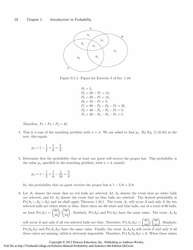
3. As seen from Fig. S.1.1, the required percentage is P1 + P2 + P3. From the given values, we have, inpercentages,




A

B

C

P1

P4

P7

P6

P3P5

P2

Figure S.1.1: Figure for Exercise 3 of Sec. 1.10.

P7 = 5,P4 = 20− P7 = 15,P5 = 20− P7 = 15,P6 = 10− P7 = 5,P1 = 60− P4 − P6 − P7 = 35,P2 = 40− P4 − P5 − P7 = 5,P3 = 30− P5 − P6 − P7 = 5.

Therefore, P1 + P2 + P3 = 45.

4. This is a case of the matching problem with n = 3. We are asked to find p3. By Eq. (1.10.10) in thetext, this equals

p3 = 1− 1

2+

1

6=

2

3.

5. Determine first the probability that at least one guest will receive the proper hat. This probability isthe value pn specified in the matching problem, with n = 4, namely

p4 = 1− 1

2+

1

6− 1

24=

5

8.

So, the probability that no guest receives the proper hat is 1− 5/8 = 3/8.

6. Let A1 denote the event that no red balls are selected, let A2 denote the event that no white ballsare selected, and let A3 denote the event that no blue balls are selected. The desired probability isPr(A1 ∪ A2 ∪ A3) and we shall apply Theorem 1.10.1. The event A1 will occur if and only if the tenselected balls are either white or blue. Since there are 60 white and blue balls, out of a total of 90 balls,

we have Pr(A1) =

(60

10

)/

(90

10

). Similarly, Pr(A2) and Pr(A3) have the same value. The event A1A2

will occur if and only if all ten selected balls are blue. Therefore, Pr(A1A2) =

(30

10

)/

(90

10

). Similarly,

Pr(A2A3) and Pr(A1A3) have the same value. Finally, the event A1A2A3 will occur if and only if allthree colors are missing, which is obviously impossible. Therefore, Pr(A1A2A3) = 0. When these values



Section 1.10. The Probability of a Union of Events 19

are substituted into Eq. (1.10.1), we obtain the desired probability,

Pr(A1 ∪A2 ∪A3) = 3

(60

10

)(90

10

) − 3

(30

10

)(90

10

) .

7. Let A1 denote the event that no student from the freshman class is selected, and let A2, A3, andA4 denote the corresponding events for the sophomore, junior, and senior classes, respectively. Theprobability that at least one student will be selected from each of the four classes is equal to 1−Pr(A1∪A2 ∪ A3 ∪ A4). We shall evaluate Pr(A1 ∪ A2 ∪ A3 ∪ A4) by applying Theorem 1.10.2. The event A1

will occur if and only if the 15 selected students are sophomores, juniors, or seniors. Since there are

90 such students out of a total of 100 students, we have Pr(A1) =

(90

15

)/

(100

15

). The values of Pr(Ai)

for i = 2, 3, 4 can be obtained in a similar fashion. Next, the event A1A2 will occur if and only if the15 selected students are juniors or seniors. Since there are a total of 70 juniors and seniors, we have

Pr(A1A2) =

(70

15

)/

(100

15

). The probability of each of the six events of the form AiAj for i < j can be

obtained in this way. Next the event A1A2A3 will occur if and only if all 15 selected students are seniors.

Therefore, Pr(A1A2A3) =

(40

15

)/

(100

15

). The probabilities of the events A1A2A4 and A1A3A4 can also

be obtained in this way. It should be noted, however, that Pr(A2A3A4) = 0 since it is impossible thatall 15 selected students will be freshmen. Finally, the event A1A2A3A4 is also obviously impossible, soPr(A1A2A3A4) = 0. So, the probability we want is

1−

⎡⎢⎢⎢⎢⎣(90

15

)(100

15

) +

(80

15

)(100

15

) +

(70

15

)(100

15

) +

(60

15

)(100

15

)

−

(70

15

)(100

15

) −

(60

15

)(100

15

) −

(50

15

)(100

15

) −

(50

15

)(100

15

) −

(40

15

)(100

15

) −

(30

15

)(100

15

) +

(40

15

)(100

15

) +

(30

15

)(100

15

) +

(20

15

)(100

15

)⎤⎥⎥⎥⎥⎦ .

8. It is impossible to place exactly n−1 letters in the correct envelopes, because if n−1 letters are placedcorrectly, then the nth letter must also be placed correctly.

9. Let pn = 1 − qn. As discussed in the text, p10 < p300 < 0.63212 < p53 < p21. Since pn is smallest forn = 10, then qn is largest for n = 10.

10. There is exactly one outcome in which only letter 1 is placed in the correct envelope, namely theoutcome in which letter 1 is correctly placed, letter 2 is placed in envelope 3, and letter 3 is placed inenvelope 2. Similarly there is exactly one outcome in which only letter 2 is placed correctly, and onein which only letter 3 is placed correctly. Hence, of the 3! = 6 possible outcomes, 3 outcomes yield theresult that exactly one letter is placed correctly. So, the probability is 3/6 = 1/2.

11. Consider choosing 5 envelopes at random into which the 5 red letters will be placed. If there are exactlyr red envelopes among the five selected envelopes (r = 0, 1, . . . , 5), then exactly x = 2r envelopes will




contain a card with a matching color. Hence, the only possible values of x are 0, 2, 4. . . , 10. Thus,for x = 0, 2, . . . , 10 and r = x/2, the desired probability is the probability that there are exactly r red

envelopes among the five selected envelopes, which is

(5

r

)(5

5− r

)(10

5

) .

12. It was shown in the solution of Exercise 12 of Sec. 1.5. that

Pr

( ∞⋃i=1

Ai

)=

∞∑i=1

Pr(Bi) = limn→∞

n∑i=1

Pr(Bi) = limn→∞Pr

(n⋃

i=1

Bi

)= lim

n→∞Pr

(n⋃

i=1

Ai

).

However, since A1 ⊂ A2 ⊂ . . . ⊂ An, it follows that⋃n

i=1Ai = An. Hence,

Pr

( ∞⋃i=1

Ai

)= lim

n→∞Pr(An).

13. We know that

∞⋂i=1

Ai =

( ∞⋃i=1

Aci

)c

.

Hence,

Pr

( ∞⋂i=1

Ai

)= 1− Pr

( ∞⋃i=1

Aci

).

However, since A1 ⊃ A2 ⊃ . . ., then Ac1 ⊂ Ac

2 ⊂ . . . . Therefore, by Exercise 12,

Pr

( ∞⋃i=1

Aci

)= lim

n→∞Pr(Acn) = lim

n→∞[1− Pr(An)] = 1− limn→∞ Pr(An).

It now follows that

Pr

( ∞⋂i=1

Ai

)= lim

n→∞Pr(An).

1.12 Supplementary Exercises


1. No, since both A and B might occur.

2. Pr(Ac ∩Bc ∩Dc) = Pr[(A ∪B ∪D)c] = 0.3.

3.

(250

18

)·(100

12

)(350

30

) .



Section 1.12. Supplementary Exercises 21

4. There are

(20

10

)ways of choosing 10 cards from the deck. For j = 1, . . . , 5, there

(4

2

)ways of choosing

two cards with the number j. Hence, the answer is(4

2

)· · ·(4

2

)(20

10

) =65(20

10

) ≈ 0.0421.

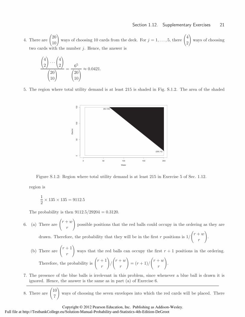
5. The region where total utility demand is at least 215 is shaded in Fig. S.1.2. The area of the shaded

Water

Ele

ctric

0 50 100 150 200

050

100

150

(65,150)

(200,15)

Figure S.1.2: Region where total utility demand is at least 215 in Exercise 5 of Sec. 1.12.

region is

1

2× 135 × 135 = 9112.5

The probability is then 9112.5/29204 = 0.3120.

6. (a) There are

(r +w

r

)possible positions that the red balls could occupy in the ordering as they are

drawn. Therefore, the probability that they will be in the first r positions is 1/

(r + w

r

).

(b) There are

(r + 1

r

)ways that the red balls can occupy the first r + 1 positions in the ordering.

Therefore, the probability is

(r + 1

r

)/

(r + w

r

)= (r + 1)/

(r + w

r

).

7. The presence of the blue balls is irrelevant in this problem, since whenever a blue ball is drawn it isignored. Hence, the answer is the same as in part (a) of Exercise 6.

8. There are

(10

7

)ways of choosing the seven envelopes into which the red cards will be placed. There




are

(7

j

)(3

7− j

)ways of choosing exactly j red envelopes and 7 − j green envelopes. Therefore, the

probability that exactly j red envelopes will contain red cards is(7

j

)(3

7− j

)/(10

7

)for j = 4, 5, 6, 7.

But if j red envelopes contain red cards, then j − 4 green envelopes must also contain green cards.Hence, this is also the probability of exactly k = j + (j − 4) = 2j − 4 matches.

9. There are

(10

5

)ways of choosing the five envelopes into which the red cards will be placed. There

are

(7

j

)(3

5− j

)ways of choosing exactly j red envelopes and 5 − j green envelopes. Therefore the

probability that exactly j red envelopes will contain red cards is(7

j

)(3

5− j

)/(10

5

)for j = 2, 3, 4, 5.

But if j red envelopes contain red cards, then j − 2 green envelopes must also contain green cards.Hence, this is also the probability of exactly k = j + ( j − 2) = 2j − 2 matches.

10. If there is a point x that belongs to neither A nor B, then x belongs to both Ac and Bc. Hence, Ac

and Bc are not disjoint. Therefore, Ac and Bc will be disjoint if and only if A ∪B = S.

11. We can use Fig. S.1.1 by relabeling the events A, B, and C in the figure as A1, A2, and A3 respectively.It is now easy to see that the probability that exactly one of the three events occurs is p1 + p2 + p3.Also,

Pr(A1) = p1 + p4 + p6 + p7,

Pr(A1 ∩ A2) = p4 + p7, etc.

By breaking down each probability in the given expression in this way, we obtain the desired result.

12. The proof can be done in a manner similar to that of Theorem 1.10.2. Here is an alternative argument.Consider first a point that belongs to exactly one of the events A1, . . . , An. Then this point will becounted in exactly one of the Pr(Ai) terms in the given expression, and in none of the intersections.Hence, it will be counted exactly once in the given expression, as required. Now consider a point thatbelongs to exactly r of the events A1, . . . , An(r ≥ 2). Then it will be counted in exactly r of the Pr(Ai)

terms, exactly

(r

2

)of the Pr(AiAj) terms, exactly

(r

3

)of the Pr(AiAjAk) terms, etc. Hence, in the

given expression it will be counted the following number of times:

r − 2

(r

2

)+ 3

(r

3

)− · · · ± r

(r

r

)

= r

[(r − 1

0

)−(r − 1

1

)+

(r − 1

2

)− · · · ±

(r − 1

r − 1

)]= 0,

by Exercise b of Sec. 1.8. Hence, a point will be counted in the given expression if and only if it belongsto exactly one of the events A1, . . . , An, and then it will be counted exactly once.



Section 1.12. Supplementary Exercises 23

13. (a) In order for the winning combination to have no consecutive numbers, between every pair ofnumbers in the winning combination there must be at least one number not in the winning com-bination. That is, there must be at least k − 1 numbers not in the winning combination to bein between the pairs of numbers in the winning combination. Since there are k numbers in thewinning combination, there must be at least k + k − 1 = 2k − 1 numbers available in order for itto be possible to have no consecutive numbers in the winning combination. So, n must be at least2k − 1 to allow consecutive numbers.

(b) Let i1, . . . , ik and j1, . . . , jk be as described in the problem. For one direction, suppose thati1, . . . , ik contains at least one pair of consecutive integers, say ia+1 = ia + 1. Then

ja+1 = ia+1 − a = ia + 1− a = ia − (a− 1) = ja.

So, j1, . . . , jk contains repeats. For the other direction, suppose that j1, . . . , jk contains repeats,say ja+1 = ja. Then

ia+1 = ja+1 + a = ja + a = ia + 1.

So i1, . . . , ik contains a pair of consecutive numbers.

(c) Since i1 < i2 < · · · < ik, we know that ia + 1 ≤ ia+1, so that ja = ia − a+ 1 ≤ ia+1 − a = ja+1 foreach a = 1, . . . , k − 1. Since ik ≤ n, jk = ik − k + 1 ≤ n − k + 1. The set of all (j1, . . . , jk) with1 ≤ j1 < · · · < jk ≤ n− k + 1 is just the number of combinations of n− k + 1 items taken k at a

time, that is

(n− k + 1

k

).

(d) By part (b), there are no pairs of consecutive integers in the winning combination (i1, . . . , ik) if

and only if (j1, . . . , jk) has no repeats. The total number of winning combinations is

(n

k

). In part

(c), we computed the number of winning combinations with no repeats among (j1, . . . , jk) to be(n− k + 1

k

). So, the probability of no consecutive integers is

(n− k + 1

k

)(n

k

) =(n− k)!(n− k + 1)!

n!(n− 2k + 1)!.

(e) The probability of at least one pair of consecutive integers is one minus the answer to part (d).



(online only mark schervish -...

Documents