optical properties of luminescent solar...
TRANSCRIPT
Optical Properties of Luminescent Solar
Concentrators
Adam Peter Green, MPhys
Submitted for the degree of
Doctor of Philosophy (Ph.D)
On completion of research at
The Department of Physics and Astronomy The University of Sheffield
Sheffield S3 7RH England
During
March 2014
i
Abstract
This thesis on luminescent solar concentrators (LSC) presents work carried out as part of the
Electronic and Photonic Molecular Materials (EPMM) group of the department of physics and
astronomy at the University of Sheffield. The work is presented in five experimental chapters looking
at a range of research aspects from film deposition and measurement instrumentation, to exploring
LSC optical properties and device performances by spectral based analytical methods.
A Gauge R & R (GRR) study design is used to assess sources of variance in an absolute fluorescence
quantum yield measurement system involving an integration sphere. The GRR statistics yield the
total variance split into three proportions; equipment, day-to-day and manufacturing variances. The
manufacturing variance, describing sample fabrication, was found to exhibit the smallest
contribution to measurement uncertainty. The greatest source of variance was found to be from
fluctuations in the laser intensity whose uncertainty is carried into the quantum yield determination
due to not knowing the exact laser intensity at the time of measurement.
The solvation phenomenon is explored as a potential way to improve LSC device yields; this occurs
due to excitation induced changes to a fluorophore's dipole moment which leads to a response by
the surrounding host medium resulting in shifts in fluorophore emission energy. This effect is shown
to improve self-absorption efficiency by reducing the overlap of absorption and emission for
particular organic fluorophores. This is expected to greatly improve energy yields but current dopant
materials are too costly to employ according to the cost evaluations of this thesis.
A spray coating deposition tool is considered for the deposition of thin film coatings for bi-layer LSC
devices. A screening study design of experiment is constructed to ascertain the level of control and
assess the tool's ability to meet thin film requirements. Despite poor control over the roughness of
the thin film layer this property was found to lie close to the acceptable roughness limit in most
samples. The biggest issue remains the film thickness achieved by the deposition, which was an order
of magnitude too small according to Beer-Lambert absorption models. This spray-coating tool is thus
unsuitable for the requirements of a bi-layer LSC.
Concentration quenching is explored in the context of LSC device efficiency. Different fluorophores
are seen to exhibited varied quenching decay strengths by looking at quantum yield versus
fluorophore concentration. For two fluorophores, 4-(Dicyanomethylene)-2-methyl-6-(4-
dimethylaminostyryl)-4H-pyran (DCM) and 2,3,6,7-Tetrahydro-9-methyl-1H,5H-quinolizino(9,1-
gh)coumarin (C102), the quenching process is explored further using quantum yield and lifetime

ii
measurements to extract the quenching rate from rate equations. The form of the quenching rate as
a function of molecular separation is shown to be of a monomial power law but distinct from the
point-like dipole-dipole coupling of Förster resonant energy transfer (FRET). Additional quenching
modes including surface-point and surface-surface interactions are considered to explain the power
law form.
Spectral analytical models have been constructed to model performance metrics for square-planar
LSC devices. In this model the input solar irradiance is considered to be incident normal to the LSC
collection face. Device thickness optimisation is explored to ensure maximisation of the absorption
efficiency by the fluorophore using Beer-Lambert absorption modelling. The normalised fluorophore
emission spectrum is converted to an equivalent irradiant intensity spectrum based on the amount of
energy absorbed. Propagation of this energy through the LSC structure is considered in terms of the
mean path length of light rays waveguided by total internal reflection and again Beer-Lambert
absorption modelling. Self-absorption and host transport losses are included in some detail. Out-
coupling of LSC irradiance at the harvesting edges to connected solar cells is then modelled, using c:Si
and GaAs power conversion efficiency spectra, and the resultant power output performance can
therefore be estimated. Comparison with real devices from literature show that the model works
reasonably well compared to these single device configurations and is somewhat conservative in its
estimates. Cost efficiency models based on reasonable assumptions conclude the scope of this work
showing that current materials fall short of delivering competitive energy solutions by at least factor
of 2 in the case of the best dye modelled here.

iii
Acknowledgements
Firstly I give my thanks to my mother, Jane Taylor, and father, Chris Green, for their encouragement
which has spurred me on to this achievement.
My sincere thanks to my supervisor, Alastair Buckley, whose guidance and patience were beyond
value, ensuring my output of research papers and the eventual completion of this thesis.
A big thanks for all the help, advice and friendship from all of my colleagues, especially to Darren
Watters, Andrew Pearson, David Coles, Edward Bovill, Jonathan Griffin, David Lidzey, James Kingsley,
Matt Watson, Lisa Hall, Aldous Everard, Giuseppe Colantuono, Jose Mawyin, Britta Kristensen and
Yimin Wang.
Also a big thank you to the department's support and technical staff for their help and invaluable
work keeping things running smoothly; particularly to Andrew Brook, Steve Collins, Richard Webb,
Paul Kerry, Pete Robinson and Chris Vickers.
Much gratitude goes to the team of workshop technicians in the department of physics and
astronomy mechanical workshop for the many tasks performed over the years.
Also thanks to the staff of the departmental office and other admin staff for their work organising
transactions, flights, maintenance payments to myself and purchases to university suppliers.
Gratitude to BASF for providing the Lumogen F series of fluorophores to the EPMM group which have
been a key material set for this thesis.
Thanks also to Cambridge Display Technologies (CDT) for providing two light emitting polymers, F8
and F8BT, to the EPMM group.
If I have left anyone out of this list please accept my apologies and my sincere thanks for your help.
iv
Contents
1. Introduction .................................................................................................................... 1
1.1. World Energy Outlook ............................................................................................... 2
1.2. Current State of Photovoltaic Solar Energy .............................................................. 4
1.3. The Case for Luminescent Solar Concentrators ........................................................ 6
1.4. Thesis Overview ........................................................................................................ 7
1.5. References ................................................................................................................. 8
2. Materials, Background and Theory ............................................................................... 11
2.1. Geometric versus Luminescent Solar Energy Concentration .................................. 11
2.2. Loss Mechanisms in Luminescent Solar Concentrators (LSC) ................................. 14
2.3. LSC Geometry and Configuration ............................................................................ 23
2.4. Semiconductor Physics for LSC Devices .................................................................. 30
2.4.1. Organic Small Molecular Fluorophores ........................................................ 35
2.4.2. Light Emitting Polymers ................................................................................ 42
2.4.3. Host Matrix Materials .................................................................................. 44
2.5. Solar Cells ................................................................................................................ 45
2.6. State of the Art LSC Devices .................................................................................... 49
2.7. References .............................................................................................................. 51
3. Experimental Methods ................................................................................................. 58
3.1. Absolute Measurement of Photoluminescence Quantum Yield ............................ 58
3.2. Determining Relative Permittivity with Impedance Spectroscopy ........................ 61
3.3. Absorption and Fluorescence Spectroscopy .......................................................... 63
3.4. Spray Coating .......................................................................................................... 65
3.5. Time Correlated Single Photon Counting (TCSPC) ................................................. 66
3.6. Spin Coating ........................................................................................................... 69
3.7. Profilometry ........................................................................................................... 69
3.8. References ..............................................................................................................71
4. Rigorous Measurement of Quantum Yield Using the Gauge Repeatability &
Reproducibility (GRR) Methodology ............................................................................ 72
4.1. Introduction ............................................................................................................ 72

v
4.2. The Gauge R & R Methodology ............................................................................... 73
4.3. Experimental Methods ........................................................................................... 75
4.4. Results and Discussion ............................................................................................ 77
4.5. Conclusions ............................................................................................................. 82
4.6. References .............................................................................................................. 83
5. Improving Luminescent Solar Concentrator Efficiency by Tuning Fluorophore Emission
with Solid State Solvation ............................................................................................ 84
5.1. Introduction ............................................................................................................ 84
5.2. Controlling the Orientational Polarisability of the Host Medium .......................... 85
5.3. Fluorophore Properties and Choice ....................................................................... 90
5.4. Optical Efficiency Predictions for the Composite Host PMMAx:CAA1-x .................. 92
5.5. Conclusions ............................................................................................................ 98
5.6. References ............................................................................................................ 100
6. Parameter Screening for Spray Coating Deposition of Surface Coated Luminescent
Solar Concentrators .................................................................................................... 102
6.1. Introduction ..........................................................................................................102
6.2. Spray Coating Parameter Space ............................................................................103
6.3. Definitions of Response Metrics ...........................................................................108
6.4. Setting Response Goals ........................................................................................ 112
6.5. Results and Discussion ......................................................................................... 117
6.5.1. Effect Leverage Analysis ............................................................................ 118
6.5.2. Desirability Analysis ................................................................................... 121
6.6. Conclusions .......................................................................................................... 126
6.7. References ........................................................................................................... 127
7. Solid State Concentration Quenching Effects for Organic Fluorophores and Implications
for LSC Devices ........................................................................................................... 128
7.1. Introduction ......................................................................................................... 128
7.2. The Impact of Host Material on Fluorescence .................................................... 129
7.3. Concentration Quenching in PMMA:DCM Systems ............................................ 133
7.4. Concentration Quenching in PMMA:C102 Systems ............................................ 138
7.5. Conclusion ........................................................................................................... 141
vi
7.6. References ........................................................................................................... 142
8. Spectral Based Models and Implications for LSC Devices ........................................ 143
8.1. Introduction ......................................................................................................... 143
8.2. The Ideal Case ...................................................................................................... 145
8.3. Predicting LSC Power Output Using a Spectral Based Approach ........................ 146
8.4. Estimating the Cost Efficiency of a LSC Device .................................................... 152
8.5. Spectral Analysis for Single Fluorophore LSC Devices ......................................... 153
8.5.1. Absorption and Self-absorption Efficiencies ............................................. 154
8.5.2. Optical Concentration ............................................................................... 156
8.5.3. Power Conversion Estimates .................................................................... 158
8.5.4. Cost Efficiency Estimates .......................................................................... 162
8.6. Conclusions .......................................................................................................... 164
8.7. References ........................................................................................................... 165
9. Conclusion ................................................................................................................. 168
9.1. Summary .............................................................................................................. 168
9.2. Implications for LSC Devices ................................................................................ 170
vii
Glossary of Constants and Notation by Chapter
Physical Constants:
Speed of Light, c = 2.99792458 x 10⁸ ms-1
Planck's Constant, h = 6.62606957 x 10⁻³⁴ m2kgs-1
Permittivity of Free Space, ε0 = 8.85418782 x 10⁻¹² Fm-1
Chapter 1:
ηPCE = Solar cell power conversion efficiency
Chapter 2:
C = Concentration ratio; for GSC use CGSC; for
LSC use CLSC
L = Irradiant power [Wm-2]; L1 for incident
light; L2 for output light
θ = Angle [°]; θ1 for acceptance angle; θ1 for
output angle;
n = Refractive index
Ω = Solid acceptance angle [Sr]
Cdye = Fluorophore concentration [mol]
ηopt = LSC optical efficiency
ηfr = Fresnel efficiency
ηtrap = Trapping efficiency
ηTIR = Total internal reflection efficiency
ηQY = Fluorescence quantum yield
ηstokes = Stokes shift efficiency
ηhost = Host light transport efficiency
ηabs = Efficiency of absorption of solar energy
ηself = Self-absorption efficiency
R = Reflected fraction; s-polarised light use Rs;
p-polarised light use Rp
T = Transmitted fraction
λ = Wavelength of light [m]
ν = Wavenumber of light [cm-1]
I(λ) = Intensity spectrum after absorption
[Wm-2nm-1]
I0(λ) = Initial incident intensity [Wm-2nm-1]
l = Mean absorption path length for incident
solar light [m]
αh(λ) = Host matrix absorption coefficient
[cm-1]
<r> = Mean path length of trapped
fluorescent irradiance [m]
<α> = Mean absorption coefficient [cm-1]
S0(λ) = Absorbed irradiance spectrum
[Wm-2nm-1]
Ssun(λ) = AM1.5 solar irradiance spectrum
[Wm-2]
S1(λ) = First order fluorescence irradiance
spectrum [Wm-2nm-1]
SN(λ) = Normalised fluorophore emission
spectrum [Wm-2nm-1]
J = Absorption-emission overlap integral
αd(λ) = Fluorophore absorption coefficients
[cm-1]
εd(λ) = Fluorophore extinction coefficients
[M-1cm-1]
Imax = Maximum intensity of fluorophore
emission spectrum
p = Integer for the pth order of emission
θc = Critical angle in the z-plane for total
internal reflection [°]
φ = Angle in the x-y plane [°]
L = LSC side length [m]
W = LSC thickness [m]
R = Cylindrical LSC radius [m]
Copt = LSC optical concentration
G = Geometric concentration
Acol = Solar energy collection area [m2]
Ahar = Solar cell harvesting area [m2]
ΔEstoke = Stokes' shift in energy [J]
viii
Δλstoke = Stokes' shift in wavelength [m]
Δν = Stokes' shift in wavenumber [cm-1]
kfl = Fluorescence decay rate [s-1]
kNR = Non-radiative decay rate [s-1]
kISC = Inter-system crossing rate [s-1]
kQ = Concentration quenching rate [s-1]
τ = Excited state decay lifetime [s]
τfl = Fluorescence lifetime [s]
τic = Internal conversion lifetime [s]
τabs = Absorption lifetime [s]
τp = Phosphorescence lifetime [s]
μG = Ground state dipole moment [D]
μG = Excited state dipole moment [D]
Δμ = Change in dipole moment [D]
Δf = Orientational polarisability
εr = Relative permittivity
a = Onsager radius [m]
Δνo = Unperturbed Stokes' shift in
wavenumbers [cm-1]
ΔEo = Unperturbed Stokes' shift in energy [J]
Mw = Molecular weight
εmax = Maximum extinction coefficient
[M-1cm-1]
ηPCE = Solar cell power conversion efficiency
ηPCE(λ) = Solar cell power conversion efficiency
spectrum
ηEQE(λ) = Solar cell external quantum
efficiency spectrum
ηex(λ) = Charge extraction efficiency
Chapter 3:
ηQY = Fluorescence quantum yield
IL,0 = Excitation intensity [counts]
IL,1 = Remaining excitation intensity [counts]
IS = Sample intensity [counts]
Iabs = Absorbed intensity [counts]
L(λ) = Laser spectrum [counts nm-1]
S(λ) = Sample and remaining laser spectrum
[counts nm-1]
C(λ) = Measured calibration lamp spectrum
[counts nm-1]
R(λ) = Radiometric calibration lamp spectrum
[μWcm-2nm-1]
φsense(λ) = Instrument sensitivity spectrum
Onorm(λ) = Normalised sample spectrum
outside sphere
Snorm(λ) = Normalised sample spectrum inside
sphere
φself(λ) = Self-absorption correction
S'(λ) = Corrected sample and remaining laser
spectrum [counts nm-1]
L'(λ) = Corrected laser spectrum [counts nm-1]
C1 = Geometric capacitance [F]
R1 = Bulk resistance [Ω]
εr = Relative permittivity
A = 4.5 x 10⁻⁶ m2, Device area
d = Film thickness
R(ω) = Frequency dependent resistance [Ω]
X(ω) = Frequency dependent reactance [Ω]
B(ω) = Frequency dependent susceptance
[Ω-1]
Cp(ω) = Frequency dependent capacitance for
parallel RC circuit [F]
T0(λ) = Blank substrate transmission spectrum
T1(λ) = Substrate and sample transmission
spectrum
Cdye = Fluorophore concentration [mol]
Sabs(λ) = Absorption spectrum
ε(λ) = Fluorophore extinction coefficients
[M-1cm-1]
<x> = Mean film thickness [m]
I(λ) = Intensity spectrum after absorption
[Wm-2nm-1]
I0(λ) = Initial incident intensity [Wm-2nm-1]
t = time
I(t) = Time-resolved intensity after absorption
[counts s-1]
I0 = Initial intensity [counts]
τ = Excited state decay lifetime [s]
Chapter 4:

ix
ηQY = Fluorescence quantum yield n = 3, Number of repeat measurements per sample o = 3, Number of days of measurement p = 5, Number of samples k = op = 15, Number of sub-groups of size n = Average range over the k subgroups R = Group range over n RURL = Upper range limit D4 = Statistical anti-biasing constant
= Repeatability variance
= Reproducibility variance
Ro = Range of o averages d2 = Bias correction factor
=
+ = Total Gauge R & R
variance
= Manufacturing variance
=
+ = Total variance
L(λ) = Laser spectrum [counts nm-1]
S(λ) = Sample and remaining laser spectrum
[counts nm-1]
φsense(λ) = Instrument sensitivity spectrum
ΔIL,0 = Excitation laser uncertainty
ΔIS = Sample emission uncertainty
ΔIL,1 = Remaining laser uncertainty
ΔηQY = Fluorescence quantum yield uncertainty
Chapter 5:
λ = Wavelength of light [m]
ν = Wavenumber of light [cm-1]
Copt = LSC optical concentration
ηopt = LSC optical efficiency
ηfr = Fresnel efficiency
ηtrap = Trapping efficiency
ηTIR = Total internal reflection efficiency
ηQY = Fluorescence quantum yield
ηstokes = Stokes shift efficiency
ηhost = Host light transport efficiency
ηabs = Efficiency of absorption of solar energy
ηself = Self-absorption efficiency
Cdye = Fluorophore concentration [g/l] and [wt%] Chost = Host concentration [g/l] CCAA = Camphoric acid anhydride concentration [wt%] Δf = Orientational polarisability
εr = Relative permittivity
n = Refractive index
ΔER = Energy lost to reaction field [J]
ΔEstoke = Stokes' shift in energy [J]
ΔEo = Unperturbed Stokes' shift in energy [J]
Δν = Stokes' shift in wavenumber [cm-1]
Δνo = Unperturbed Stokes' shift in
wavenumbers [cm-1]
νPL = Peak emission wavenumber [cm-1]
νabs = Peak absorption wavenumber [cm-1]
μG = Ground state dipole moment [D]
μG = Excited state dipole moment [D]
Δμ = Change in dipole moment [D]
a = Onsager radius [Å]
J = Absorption-emission overlap integral
G = Geometric concentration
p = Integer for the pth order of emission
m = Gradient of lines on Fig. 5.4.4
Chapter 6:
<RR> = Roughness ratio
σR = Standard deviation of <RR>
Rh = Height Range [m]
<t> = Mean film thickness [m]
Iabs = Relative absorption intensity
Δw = De-broadening parameter [m]
w = Full width at half maximum [m]
λ = Wavelength of light [m]
ΔλPL = Change in Stokes' shift [m]
G = Geometric concentration
n = Refractive index
Cdye = Fluorophore concentration [wt%]
Ctot = Host + fluorophore concentration [g/l]
Pin = Spray head pressure [mbar]
T = Temperature [°C]
h = Spray head to substrate distance [mm]

x
s = Spray head lateral speed [mms-1]
Ncoat = Number of coats
ηfr = Fresnel efficiency
ηTIR = Total internal reflection efficiency
ηabs = Efficiency of absorption of solar energy
ηQY = Fluorescence quantum yield
<Δh> = Mean height between peaks [m]
<Δx> = Mean distance between peaks [m]
Sabs(λ) = Absorption spectrum
NA = Numerical Aperture
D = Derringer-Suich desirability function
di = ith individual response desirability
function
Dmax = Maximum desirability
Dmin = Minimum desirability
Chapter 7:
ηQY = Fluorescence quantum yield
τ = Excited state decay lifetime [s]
r = Mean molecular separation
Cdye = Fluorophore concentration [g/l] and [M]
Chost = Host concentration [g/l]
Mw = Molecular weight
ηfr = Fresnel efficiency
ηtrap = Trapping efficiency
kFRET = Förster resonant energy transfer rate
[s-1]
r0 = Förster radius [m]
τ0 = Intrinsic decay lifetime of fluorescence
state [s]
kET = Point-surface interaction energy transfer
rate [s-1]
ṟ0 = Radius for point-surface interaction [m]
ρ = Fluorophore density
kQ = Concentration quenching rate [s-1]
kfl = Fluorescence decay rate [s-1]
kNR = Non-radiative decay rate [s-1]
a = Onsager radius [Å]
Chapter 8:
n = Refractive index
λ = Wavelength of light [m]
εr = Relative permittivity
Copt = LSC optical concentration
ηopt = LSC optical efficiency
ηLSC = LSC power conversion efficiency
ηfr = Fresnel efficiency
ηtrap = Trapping efficiency
η'trap = Corrected trapping efficiency
ηTIR = Total internal reflection efficiency
ηQY = Fluorescence quantum yield
ηstokes = Stokes shift efficiency
ηhost = Host light transport efficiency
ηabs = Efficiency of absorption of solar energy
ηself = Self-absorption efficiency
ηPCE = Solar cell power conversion efficiency
ηPCE(λ) = Solar cell power conversion efficiency
spectrum
ηEQE(λ) = Solar cell external quantum
efficiency spectrum
ηex(λ) = Charge extraction efficiency
SLSC(λ) = LSC output irradiance spectrum [Wm-
2]
Ssun(λ) = AM1.5 solar irradiance spectrum
[Wm-2]
SN(λ) = Normalised fluorophore emission
spectrum [Wm-2nm-1]
S0(λ) = Absorbed irradiance spectrum
[Wm-2nm-1]
Sp(λ) = pth order fluorescence irradiance
spectrum [Wm-2nm-1]
SECL(λ) = Escape cone irradiance spectrum
[Wm-2]
Strap(λ) = Trapped irradiance spectrum [Wm-2]
p = Integer for the pth order of emission
Pin = Power into LSC device from sun [W]
Pout = Power out of LSC device [W]
xi
PN = Relative output power
G = Geometric concentration
L = LSC side length [m]
W = LSC thickness [m]
<r> = Mean path length of trapped
fluorescent irradiance [m]
l = Mean absorption path length for incident
solar light [m]
ε(λ) = Fluorophore extinction coefficients [M-
1cm-1]
T(λ) = Transmitted irradiance
θi = Solar irradiance incidence angle [°]
θc = Critical angle in the z-plane for total
internal reflection [°]
θECL = Average angle in z-plane of escape cone
light [°]
αd(λ) = Fluorophore absorption coefficients
[cm-1]
Cdye = Fluorophore concentration [M]
Ahar = Harvesting area [m2]
Acol = Collection area [m2]
VLSC = LSC Volume [m3]
(£/W)conc = LSC cost per unit power delivered
[£ W-1]
(£host/m3) = Cost of host materials per unit
concentrator volume [£ m-3]
(£dye/mol) = Cost of dye materials per unit
concentration [£ mol-1]
(£PV/m2) = Cost of solar cells per unit area [£
m-2]
ρPMMA = Density of PMMA [kg m-3]
J = Absorption-emission overlap integral
xii
List of Figures
1. Figure 1.1: Types of Solar Energy .............................................................................. 1
2. Figure 2.1.1: GSC Concentration Ratio ..................................................................... 13
3. Figure 2.2.1: LSC Schematic Diagram ....................................................................... 15
4. Figure 2.2.2: Fractional Transmission vs. n for LSC .................................................. 16
5. Figure 2.2.3: Fractional Transmission vs. Incidence Angle for LSC ........................... 17
6. Figure 2.2.4: Fractional Efficiency ηfrηtrap vs n for LSC .............................................. 18
7. Figure 2.4.1: State Configuration Diagram ............................................................... 31
8. Figure 2.4.2: Perylene Absorption and Emission with FC Factors ............................ 32
9. Figure 2.4.3: General Luminophore Jablonski Diagram ........................................... 33
10. Figure 2.4.4: Jablonski Diagram with Solvation Mechanism .................................... 34
11. Figure 2.4.5: Spectra of Coumarin 102 ..................................................................... 37
12. Figure 2.4.6: Spectra of Perylene ............................................................................. 38
13. Figure 2.4.7: Spectra of Perylene Red ...................................................................... 38
14. Figure 2.4.8: Spectra of Perylene Orange ................................................................ 38
15. Figure 2.4.9: Spectra of DCM ................................................................................... 39
16. Figure 2.4.10: Spectra of DCM2 ............................................................................... 39
17. Figure 2.4.11: Spectra of DCJTB ............................................................................... 39
18. Figure 2.4.12: Spectra of DANS ................................................................................ 40
19. Figure 2.4.13: Spectra of Phenoxazine 660 .............................................................. 40
20. Figure 2.4.14: Spectra of Rhodamine 6G ................................................................. 40
21. Figure 2.4.15: Spectra of ADS067RE ......................................................................... 41
22. Figure 2.4.16: Spectra of Pyridine 1 ......................................................................... 41
23. Figure 2.4.17: Spectra of Pyridine 2 ......................................................................... 41
24. Figure 2.4.18: Spectra of F8 ..................................................................................... 42
25. Figure 2.4.19: Spectra of F8BT ................................................................................. 43
26. Figure 2.4.20: Spectra of ADS111RE ........................................................................ 43
27. Figure 2.5.1: GaAs Efficiency vs. Concentration ...................................................... 46
28. Figure 2.5.2: EQE Spectra of Various Solar Cells ...................................................... 47
29. Figure 2.5.3: PCE Spectra of Various Solar Cells ....................................................... 48
30. Figure 2.5.4: Power Correction Factor vs Optical Concentration ............................. 49
xiii
31. Figure 3.1.1: Schematic of Integration Sphere Measurement of ηQY ...................... 59
32. Figure 3.2.1: ITO Substrate and EC Diagram ............................................................ 61
33. Figure 3.2.2: Impedance Analysis, Capacitance vs. Frequency Plot ......................... 62
34. Figure 3.3.1: Schematic Diagram of Fluoromax-4 Spectrofluorometer ................... 63
35. Figure 3.4.1: Photograph of Prism Ultra-Coat 300 Spray Coater ............................. 66
36. Figure 3.5.1: Schematic Diagram of the TCSPC setup .............................................. 68
37. Figure 3.5.2: TCSPC Instrument Response Function ................................................ 68
38. Figure 4.3.1: Raw Integration Sphere Data Plot ....................................................... 75
39. Figure 4.4.1: Variability Chart for F8 ........................................................................ 77
40. Figure 4.4.2: Variability Chart for Perylene .............................................................. 79
41. Figure 4.4.3: Variability Chart for Perylene Red ....................................................... 80
42. Figure 4.4.4: Laser Flux Magnitude Distributions ..................................................... 81
43. Figure 5.2.1: Orientational Polarisability of Common Host Materials ..................... 86
44. Figure 5.2.2: Relative Permittivity vs. CCAA in PMMA ............................................... 88
45. Figure 5.3.1: 3D Colour Map of Stokes' Shift vs. Fluorophore Properties ................ 91
46. Figure 5.4.1: Spectra for DCM and DCM2 in PMMAx:CAAx-1 .................................... 93
47. Figure 5.4.2: Spectra for DCJTB in PMMAx:CAAx-1 and The Zero Polarity Curve ...... 93
48. Figure 5.4.3: ηopt and ηQY vs. CCAA in PMMA .............................................................. 94
49. Figure 5.4.4: Stokes' Shift vs. Orientational Polarisability ....................................... 95
50. Figure 5.4.5: Stokes' Shift vs. Relative Permittivity .................................................. 98
51. Figure 6.2.1: Schematic Infographic of Spray Deposition ....................................... 104
52. Figure 6.2.2: Photographs of S09 and S10 .............................................................. 106
53. Figure 6.3.1: Annotated Photograph of Sprayed Sample S01 ................................. 108
54. Figure 6.3.2: Smoothed Surface Profile of Sample S01 ........................................... 109
55. Figure 6.3.3: Relative Intensity Absorption Spectra of DCJTB ................................. 110
56. Figure 6.3.4: Relative Intensity Absorption Spectra of Perylene Red ..................... 110
57. Figure 6.3.5: Schematic of Self-Absorption Measurement Setup ........................... 111
58. Figure 6.3.6: Acquisition Edge Emission Spectra of Sample S02 ............................. 112
59. Figure 6.4.1: Beer-Lambert Absorption of AM1.5 Spectrum by DCJTB ................... 115
60. Figure 6.4.2: Beer-Lambert Absorption of AM1.5 Spectrum by Perylene Red ........ 115
61. Figure 6.4.3: LSC Efficiency Estimator ηabsηQY for Cdye Optimisation ....................... 116
62. Figure 6.5.1: Full Model Leverage Plots for Roughness Response Metrics ............. 118

xiv
63. Figure 6.5.2: Full Model Leverage Plots for Absorption Response Metrics ............. 119
64. Figure 6.5.3: Leverage Plots for Iabs vs. Cdye and s .................................................... 120
65. Figure 6.5.4: Full Model Leverage Plots for Self-Absorption Response Metrics ..... 120
66. Figure 6.5.5: Relative Intensity Self-Absorption Spectra for DCJTB ........................ 123
67. Figure 6.5.6: Full Model Prediction Profiler ............................................................ 125
68. Figure 7.2.1: ηQY vs. Cdye for Various Fluorophores in PMMA .................................. 129
69. Figure 7.2.2: ηQY vs. Cdye and r for DCM2 in PMMA with Various MW ..................... 130
70. Figure 7.2.3: ηQY vs. Cdye and r for DCM in Various Hosts ........................................ 131
71. Figure 7.2.4: τ vs. Cdye for DCM in Various Acrylic Hosts ......................................... 132
72. Figure 7.2.5: ηQY and τ vs. Cdye for DCM in PMMA .................................................. 133
73. Figure 7.3.1: ηQY and τ vs. r for DCM in PMMA ...................................................... 134
74. Figure 7.3.2: kfl and kNR + kQ vs. r for DCM in PMMA .............................................. 135
75. Figure 7.3.3: kQ vs. r for DCM in PMMA .................................................................. 136
76. Figure 7.4.1: ηQY and τ vs. r for Coumarin 102 in PMMA ....................................... 138
77. Figure 7.4.2: kfl and kNR + kQ vs. r for Coumarin 102 in PMMA ............................... 139
78. Figure 7.4.3: kQ vs. r for Coumarin 102 in PMMA ................................................... 140
79. Figure 8.3.1: PCE Spectra with Marked Fluorophore Emission Peaks .................... 147
80. Figure 8.3.2: Predicted Irradiance Spectra for Perylene Red .................................. 149
81. Figure 8.5.1: AM1.5 and Model Irradiance Spectra for DCJTB ................................ 154
82. Figure 8.5.2: Modelled ηabs vs. LSC Thickness, W .................................................... 155
83. Figure 8.5.3: Modelled ηself vs. LSC Side Length, L ................................................... 156
84. Figure 8.5.4: Modelled ηopt vs. Acol and G ................................................................ 157
85. Figure 8.5.5: Modelled Pout vs. Acol .......................................................................... 158
86. Figure 8.5.6: Modelled ηLSC vs. Acol .......................................................................... 159
87. Figure 8.5.7: Modelled ηLSC vs. Acol for Various n .................................................... 162
88. Figure 8.5.8: Modelled ηLSC and (£/W)conc vs. Acol ................................................... 162
89. Figure 8.5.9: Modelled LSC Component Costs vs. L ................................................ 163
xv
List of Tables
1. Table I: ηPCE for Various Solar Cell Devices and Modules ........................................... 5
2. Table II: Organic Fluorophore Properties in PMMA ................................................. 37
3. Table III: Light Emitting Polymer Properties ............................................................. 43
4. Table IV: Properties for Various Host Materials ....................................................... 45
5. Table V: ηPCE Values for Various Accredited Research Solar Cells ............................ 46
6. Table VI: A Pick of the Best LSC Devices in Literature .............................................. 50
7. Table VII: Gauge R & R Statistics .............................................................................. 77
8. Table VIII: Gauge R & R Uncertainties ...................................................................... 79
9. Table IX: Error Analysis Summary ............................................................................. 81
10. Table X: Host Media Optical Properties ................................................................... 86
11. Table XI: Solvation Results Summary ....................................................................... 96
12. Table XII: Parameter Screening Design of Experiment ........................................... 107
13. Table XIII: Response Metric Goals for Desirability Analysis .................................... 113
14. Table XIV: Whole Model Statistics and Significant Factors ..................................... 121
15. Table XV: Desirability Analysis Summary ................................................................ 122
16. Table XVI: Predicted Factors for Min and Max Desirability .................................... 124
17. Table XVII: Ideal LSC Optical Concentration Parameters ........................................ 145
18. Table XVIII: Relative Output Power for Various LSC/Solar Cell Combinations ...... 147
1
Chapter 1
Introduction
Solar energy offers a renewable resource that is both abundant and available across the entire
surface of the world. It has potential for a wide range of applications such as large scale power
generation, small scale generation for local deployment and building integrated applications. A
number of solar energy technologies are currently available which can be broadly grouped into
direct and concentrated solar energy systems. Under direct illumination photovoltaic (PV) solar cell
modules already offer competitive energy solutions for large and small scale generation systems but
lack option for building integrated applications.
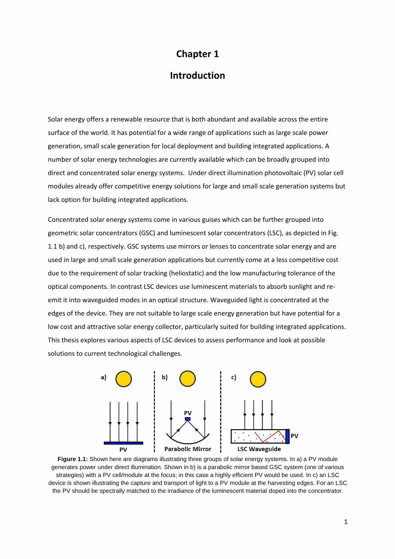
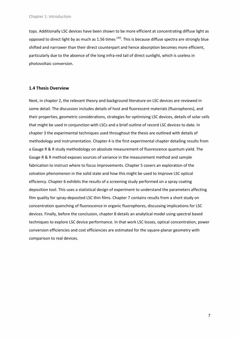
Concentrated solar energy systems come in various guises which can be further grouped into
geometric solar concentrators (GSC) and luminescent solar concentrators (LSC), as depicted in Fig.
1.1 b) and c), respectively. GSC systems use mirrors or lenses to concentrate solar energy and are
used in large and small scale generation applications but currently come at a less competitive cost
due to the requirement of solar tracking (heliostatic) and the low manufacturing tolerance of the
optical components. In contrast LSC devices use luminescent materials to absorb sunlight and re-
emit it into waveguided modes in an optical structure. Waveguided light is concentrated at the
edges of the device. They are not suitable to large scale energy generation but have potential for a
low cost and attractive solar energy collector, particularly suited for building integrated applications.
This thesis explores various aspects of LSC devices to assess performance and look at possible
solutions to current technological challenges.
Figure 1.1: Shown here are diagrams illustrating three groups of solar energy systems. In a) a PV module
generates power under direct illumination. Shown in b) is a parabolic mirror based GSC system (one of various
strategies) with a PV cell/module at the focus; in this case a highly efficient PV would be used. In c) an LSC
device is shown illustrating the capture and transport of light to a PV module at the harvesting edges. For an LSC
the PV should be spectrally matched to the irradiance of the luminescent material doped into the concentrator.
Chapter 1: Introduction
2
1.1 World Energy Outlook
According to the International Energy Agency's (IEA) World Energy Outlook 2013 [1], global primary
energy demand is expected to increase by around 21% by 2035, reaching 200 trillion kWh yr-1.
During this 20 year period fossil fuel production and usage, particularly in natural gas development,
is set to rise, though proportionally the share for renewable energy will increase by several percent.
The BP Energy Outlook 2035 estimates a 14% global share in renewable energy sources by 2035, up
from 5% in 2012 [2]. They also estimate a 41% increase in global energy demand, quite different to
IEA predictions.
Currently fossil fuels account for 82% of primary energy use and are heavily subsidised; a total global
subsidy of $544 Billion was given in 2012 according to the IEA, which poses a significant obstacle for
renewable energy to penetrate the market and gain a larger share. According to a 2012 report from
Global Subsidies Initiative (GSI), a group founded by the International Institute for Sustainable
Development (IISD), this figure could be as high as $750 Billion but there are large uncertainties due
to poor accountancy and/or transparency on these figures [3]. The definition of a fossil fuel subsidy
remains vague as much of the funds being spent on the industry do not fall into the category of a
normal subsidy, which is generally a state fund to help an industry keep prices low. Large parts of
these funds are actually tax exemptions for mining companies, energy producers or consumers,
which result in lost national revenue that is equivalent to providing a subsidy. Unfortunately removal
of these tax exemptions has some severe knock-on effects with rising petrol prices being a key one
as this can lead to economic decline and job losses, often met by bitter protest [4].The GSI report
expressed hope for fossil fuel subsidy reform to be a key agenda for the Rio+20 summit of that same
year [5] with a target for total global subsidy reform set at 2020. However, despite reaffirmations of
commitment to take action on this matter at Rio+20, there is little sign of real progress [4].
With fossil fuel energy share remaining high for decades to come, IEA and Intergovernmental Panel
for Climate Change (IPCC) predictions make for gloomy reading with a highly likely increase in global
average temperature exceeding the internationally agreed upon maximum of 2°C for dangerous
climate change. The IPCC, releasing the Climate Change 2013 report last year [6] and their fifth
assessment report this year (March/April 2014), has led calls for a more radical global effort to be
made. However, such bold action would require bold leadership, lacking in the political sphere
rather than in the scientific one. It would also require bold financing; a Forbes analysis calls for a
shift to a 1/3-1/3-1/3 scenario where a third of global energy demand is provided by each of fossil
fuels, renewable energy and nuclear. They predict a total cost to achieve this would be around $65
trillion over the next 50 years [7]; the scale of such a global project is unimaginable with current
Chapter 1: Introduction
3
political leadership. This figure is somewhat higher than the current global public debt burden which
is at around $57 trillion and rising.
Many countries are beginning to set ambitious targets on renewable energy, and some already
achieve ambitious goals. Denmark approaches the point of generating all of its power by wind alone,
as it did at a time of low power consumption in November 2013 [8]. Over December 2013 wind
power provided 52% of the country's consumption. However, the situation is more complex because
wind capacity is also being imported from Germany, and exported from Denmark to the other
Scandinavian countries. Denmark benefits from large wind resources, plus a population of only 5.6
million, and will likely reach 100% renewable energy share by 2050.
Germany has increased its wind and solar capacity considerably but various problems have arisen
due to installing renewable capacity without proper planning of grid infrastructure [9]. Grid
instabilities due to too much power being delivered at times of low consumption, particularly with
large wind farms in East Germany, threaten blackouts and large energy exports to Eastern Europe
and Scandinavia have been necessary to control the situation. Since 2013 Germany now produces
around 4% of its power from solar energy, making it the largest solar generator in the world at this
time, with aims to produce 35% from renewables by 2020 and 100% by 2050 [11]. It faces greater
challenge than Denmark in this, however, with a population of 82 million and a much larger fossil
fuel share, which is still being subsidised. According to the GSI report Germany spent €7.4 billion on
fossil fuel subsidies in 2010 [3].
Spain has spent a lot of capital with aggressive subsidies to introduce renewables widely and has
become one of the big producers of wind, hydroelectric and solar energy in Europe. In 2013 20% of
the power consumption was delivered from wind power and 3.1% from solar energy marking
significant progress in the transition to renewable energy [11]. The result of aggressive subsidisation,
high feed-in-tariffs and a complex interplay with lower cost non-renewable sources has left the
Spanish power market with a huge financial deficit [12]. This has unfortunately broken confidence in
renewable energy in Spain and offers a cautionary tale. However, complexities including the fact
that fossil fuels are heavily subsidised should be considered. According to the GSI report Spain spent
€2.6 billion on fossil fuel subsidies in 2010 [3].
China has woken up to the consequences of having 90% of its primary energy delivered by coal and
has set the target of achieving 15% renewable energy share by 2020 [13], with more to follow in five
year plans. In 2012 the renewable share in China was already 9%, largely from hydroelectric and
wind power, and plans to install more wind and solar capacity are in motion. By comparison in 2013
Chapter 1: Introduction
4
the US produced 9% of total power requirements from renewable energy showing a slower uptake
in the more mature, fossil fuel dominated energy market of the US [3].
The world's energy mix will continue to change slowly towards renewable energy in a dynamic and
sometimes chaotic manner. The success of introduction of renewable energy has been mixed with
problems arising from poor planning of infrastructure, intermittent power supply and subsidisation
issues. As long as fossil fuel subsidies remain high a true renewable energy revolution to curb
dangerous climate change will not be possible.
1.2 The Current State of Photovoltaic Solar Energy
Solar energy currently accounts for less than 1% of the world's primary energy demand and this
capacity is mostly comprised of silicon based photovoltaics (PV) with some concentrated solar power
plants, particularly in Spain and Australia, and solar thermal installations. Polysilicon feedstock prices
have been increasing due to oversupply after the economic crisis in 2008 and, according to GTM
Research's Global PV Pricing Outlook 2014, global PV module prices are set to rise by about 9% this
year since the PV supply chain stabilised in 2013 [14]. Module prices are forecast to resume the
gradual decline of previous years down to around 0.5 $/W for Chinese Tier 1 manufacturers during
2015 and after. As a result competition remains very tight for emerging technologies to penetrate
the solar energy market and it seems unlikely that this could happen on a large scale unless a major
breakthrough is made. In 2012 China held a 60% share in global PV production whereas the vast
majority of demand currently lies in Europe [15].
Photovoltaic technology has come a long way since the first recorded devices of the 1970's with
further development of 'classical' photovoltaic technologies and the emergence of many new ones.
Classically there are two groups; first are single crystal inorganic semiconductor PV devices, made
from Si and GaAs, and second are inorganic thin film PV devices using CdTe, CuInGaSe (CIGS) and
amorphous silicon (a:Si). Today many new technologies have emerged including multi-junction
inorganic PV, organic semiconductors, multicrystalline silicon (mc:Si), nanomaterials, dye sensitised
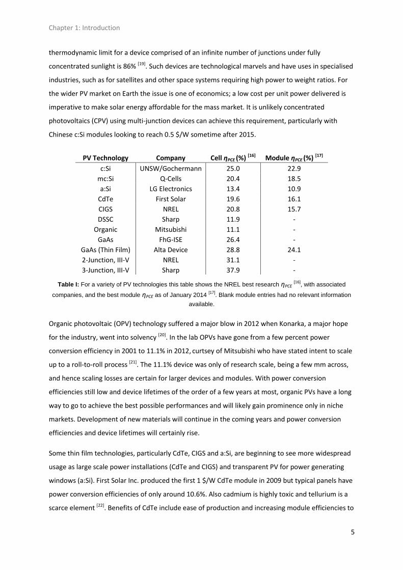
solar cells (DSSC) and nanocrystals. The best current laboratory and module power conversion
efficiencies, ηPCE, for a number of PV technologies are given in Table I. ηPCE is defined as the ratio of
the power out to the power in (see chapter 2.5).
Multi-junction cells have reached efficiencies of up to 44.4% in 2013; this was a triple-junction PV
device made by Sharp that utilises concentrator technology to achieve 302 suns [18]. The
Chapter 1: Introduction
5
thermodynamic limit for a device comprised of an infinite number of junctions under fully
concentrated sunlight is 86% [19]. Such devices are technological marvels and have uses in specialised
industries, such as for satellites and other space systems requiring high power to weight ratios. For
the wider PV market on Earth the issue is one of economics; a low cost per unit power delivered is
imperative to make solar energy affordable for the mass market. It is unlikely concentrated
photovoltaics (CPV) using multi-junction devices can achieve this requirement, particularly with
Chinese c:Si modules looking to reach 0.5 $/W sometime after 2015.
PV Technology Company Cell ηPCE (%) [16] Module ηPCE (%) [17]
c:Si UNSW/Gochermann 25.0 22.9
mc:Si Q-Cells 20.4 18.5
a:Si LG Electronics 13.4 10.9
CdTe First Solar 19.6 16.1
CIGS NREL 20.8 15.7
DSSC Sharp 11.9 -
Organic Mitsubishi 11.1 -
GaAs FhG-ISE 26.4 -
GaAs (Thin Film) Alta Device 28.8 24.1
2-Junction, III-V NREL 31.1 -
3-Junction, III-V Sharp 37.9 -
Table I: For a variety of PV technologies this table shows the NREL best research ηPCE [16]
, with associated
companies, and the best module ηPCE as of January 2014 [17]
. Blank module entries had no relevant information
available.
Organic photovoltaic (OPV) technology suffered a major blow in 2012 when Konarka, a major hope
for the industry, went into solvency [20]. In the lab OPVs have gone from a few percent power
conversion efficiency in 2001 to 11.1% in 2012, curtsey of Mitsubishi who have stated intent to scale
up to a roll-to-roll process [21]. The 11.1% device was only of research scale, being a few mm across,
and hence scaling losses are certain for larger devices and modules. With power conversion
efficiencies still low and device lifetimes of the order of a few years at most, organic PVs have a long
way to go to achieve the best possible performances and will likely gain prominence only in niche
markets. Development of new materials will continue in the coming years and power conversion
efficiencies and device lifetimes will certainly rise.
Some thin film technologies, particularly CdTe, CIGS and a:Si, are beginning to see more widespread
usage as large scale power installations (CdTe and CIGS) and transparent PV for power generating
windows (a:Si). First Solar Inc. produced the first 1 $/W CdTe module in 2009 but typical panels have
power conversion efficiencies of only around 10.6%. Also cadmium is highly toxic and tellurium is a
scarce element [22]. Benefits of CdTe include ease of production and increasing module efficiencies to
Chapter 1: Introduction
6
16% (see Table I). CIGS panels have produced efficiencies of 12 to 16% and costs are expected to fall
below 1 $/W by 2014 according to a nanomarkets.net whitepaper [23]. Despite these encouraging
developments the PV market has faced some overcapacity and thin film PV market share is expected
to suffer as a result. In 2009 thin film PV claimed a 16% share in global PV production but this is
expected to drop to around 7% during 2017 [24].
The stage seems set for c:Si and mc:Si technologies to dominate the PV market for decades to come
with other technologies taking back seat or niche roles. These niche roles are a motivating focus in
this thesis regarding the luminescent solar concentrator technology.
1.3 The Case for Luminescent Solar Concentrators
LSC devices can theoretically achieve the same conversion efficiency as a single junction PVs [25] but
suffer from a larger number of loss mechanisms. These losses in the LSC system mean that typical
power conversion efficiencies will be lower than standard PV modules under direct solar irradiance.
The LSC is therefore unlikely to see a leading role in the global solar energy market.
However, it may be possible to reduce LSC cost significantly enough to make it cost competitive,
which is a core research goal for LSC devices. Combined with commonly available materials and ease
of processing there is opportunity to develop a useful, low-resource intensity device that could find
place in niche markets. Key markets lie in building integrated solar applications where coloured
concentrators could create aesthetically pleasing structures whilst generating power for local utility.
Many ideas for building integration are in circulation including energy fixtures in bus-stop roofs,
paving, awnings, windows and sound barriers [26].
Further non-power generation applications include waveguides for indoor day lighting [27] and
thermal energy capture [28, 29]. This latter application utilises one of the most useful properties of the
LSC where thermal energy from the sun is separated from the visual wavelengths and dissipated in
the bulk of the concentrator. This thermal energy could be utilised with a heat exchange system
underneath the concentrator to heat water or indoor spaces.
LSC devices offer some advantage over standard geometric solar concentrators (GSC) using mirrors
or lenses. They readily accept diffuse light to large solid angles, as shall be detailed in chapter 2, and
as such require no heliostatic tracking systems, which add significant cost. This point is moot for
power plant scale solar energy projects since the LSC can hardly replace heliostat arrays. However,
the LSC could gain significant share for small scale, terrestrial concentrated solar applications on roof
Chapter 1: Introduction
7
tops. Additionally LSC devices have been shown to be more efficient at concentrating diffuse light as
opposed to direct light by as much as 1.56 times [30]. This is because diffuse spectra are strongly blue
shifted and narrower than their direct counterpart and hence absorption becomes more efficient,
particularly due to the absence of the long infra-red tail of direct sunlight, which is useless in
photovoltaic conversion.
1.4 Thesis Overview
Next, in chapter 2, the relevant theory and background literature on LSC devices are reviewed in
some detail. The discussion includes details of host and fluorescent materials (fluorophores), and
their properties, geometric considerations, strategies for optimising LSC devices, details of solar cells
that might be used in conjunction with LSCs and a brief outline of record LSC devices to date. In
chapter 3 the experimental techniques used throughout the thesis are outlined with details of
methodology and instrumentation. Chapter 4 is the first experimental chapter detailing results from
a Gauge R & R study methodology on absolute measurement of fluorescence quantum yield. The
Gauge R & R method exposes sources of variance in the measurement method and sample
fabrication to instruct where to focus improvements. Chapter 5 covers an exploration of the
solvation phenomenon in the solid state and how this might be used to improve LSC optical
efficiency. Chapter 6 exhibits the results of a screening study performed on a spray coating
deposition tool. This uses a statistical design of experiment to understand the parameters affecting
film quality for spray-deposited LSC thin films. Chapter 7 contains results from a short study on
concentration quenching of fluorescence in organic fluorophores, discussing implications for LSC
devices. Finally, before the conclusion, chapter 8 details an analytical model using spectral based
techniques to explore LSC device performance. In that work LSC losses, optical concentration, power
conversion efficiencies and cost efficiencies are estimated for the square-planar geometry with
comparison to real devices.
Chapter 1: Introduction
8
1.5 References
[1] World Energy Outlook 2013, International Energy Agency (IEA) (2013),
http://www.worldenergyoutlook.org/
[2] Energy Outlook 2035, British Petroleum Plc. (BP) (2014),
http://www.bp.com/content/dam/bp/pdf/Energy-economics/Energy-
Outlook/Energy_Outlook_2035_booklet.pdf
[3] Fossil fuel subsidies and government support in 24 OECD countries, Global Subsidies Initiative
(GSI) (2012), http://www.iisd.org/gsi/news/report-highlights-fossil-fuel-subsidies-24-oecd-countries
[4] R. Andersen, Business Reporter, BBC News (2014),
http://www.bbc.co.uk/news/business-27142377
[5] The Future We Want - Outcome Document, Sustainable Development Knowledge Platform,
United Nations (UN) (2012), http://sustainabledevelopment.un.org/index.php?menu=1298
[6] Climate Change 2013: The Physical Science Basis, Intergovernmental Panel for Climate Change
(IPCC) (2013), http://www.ipcc.ch/report/ar5/wg1/#.Uvv4_LQa6tM
[7] James Conca, What is Our Energy Future?, Forbes (2012),
http://www.forbes.com/sites/jamesconca/2012/05/13/what-is-our-energy-future/
[8] Craig Morris, Denmark Surpasses 100 Percent Wind Power, Energy Transition (2013),
http://energytransition.de/2013/11/denmark-surpasses-100-percent-wind-power/
[9] Richard Fuchs, Wind Energy Surplus Threatens Eastern German Power Grid, Euro Dialogue
(2011), http://eurodialogue.org/Wind-energy-surplus-threatens-eastern-German-power-grid
[10] Paul Hockenos, Germany's Grid and the Market: 100 Percent Renewable by 2050?, Renewable
Energy World (2012), http://www.renewableenergyworld.com/rea/blog/post/2012/11/ppriorities-
germanys-grid-and-the-market
[11] Peter Moskowitz, Spain becomes first country to rely mostly on wind for energy, Al Jazeera
(2014), http://america.aljazeera.com/articles/2014/1/16/spain-becomes-
firstcountrytorelymostlyonwindforenergy.html
Chapter 1: Introduction
9
[12] Andrés Cala, Renewable Energy in Spain is Taking a Beating, New York Times (2013),
http://www.nytimes.com/2013/10/09/business/energy-environment/renewable-energy-in-spain-is-
taking-a-beating.html?_r=1&
[13] Josh Bateman, The New Global Leader in Renewable Energy, Renewable Energy World (2014),
http://www.renewableenergyworld.com/rea/news/article/2014/01/the-new-global-leader-in-
renewable-energy
[14] Global PV Pricing Outlook 2014, Green Tech Media Research (2013),
http://www.greentechmedia.com/research/report/pv-pricing-outlook-2014
[15] Finlay Colville and Steven Han, Solar PV Supply and Demand within Emerging Asian Countries,
Solar Media Ltd. (2013), http://www.solarbusinessfocus.com/articles/solar-pv-supply-and-demand-
within-emerging-asian-countries
[16] Best Research PCE Values, NREL (2013), http://www.nrel.gov/ncpv/
[17] M. A. Green, K. Emery, Y. Hishikawa, W. Warta and E. D. Dunlop, Solar Cell Efficiency Tables
(version 43), Prog. Photovolt: Res. Appl. 22, 1, 1 - 9 (2014)
[18] Eric Wesoff, Sharp Hits Record 44.4% Efficiency for Triple-Junction Solar Cell, Green Tech Media
(2013), http://www.greentechmedia.com/articles/read/Sharp-Hits-Record-44.4-Efficiency-For-
Triple-Junction-Solar-Cell
[19] J. Nelson, The Physics of Solar Cells, (Imperial College Press, London, 2003), Chap. 10, pp. 289 -
301
[20] Ucilia Wang, Organic solar thin film maker Konarka files for bankruptcy, GIGAOM, Wordpress
(2012), http://gigaom.com/2012/06/01/solar-thin-film-maker-konarka-files-for-bankruptcy/
[21] Tetsuo Nozawa (Nikkei Electronics), Mitsibishi Chemical Claims Efficiency Record for Organic
Thin-film PV Cell, TechOn! (2012),
http://techon.nikkeibp.co.jp/english/NEWS_EN/20120601/221131/
[22] Solar Facts and Advice, Alchemie Limited Inc.(2010-2013) http://www.solar-facts-and-
advice.com/cadmium-telluride.html
[23] Glen Allen, Renewed Interest in CIGS Creating Real Opportunities in Photovoltaics,
Nanomarkets.net (2011), http://nanomarkets.net/Downloads/CIGSPaper.pdf
Chapter 1: Introduction
10
[24] Mark Osborne, NPD Solarbuzz: CIGS suffering in a PV thin-film market decline, PV Tech (2013),
http://www.pv-tech.org/news/npd_solarbuzz_cigs_suffering_in_a_pv_thin_film_market_in_decline
[25] Tom Markvart, Detailed Balance Method for Ideal Single-Stage Fluorescent Collectors, J. App.
Phys. 99, (2006)
[26] Michael G. Debije and Paul P. C. Verbunt, Thirty Years of Luminescent Solar Concentrator
Research: Solar Energy for the Built Environment, Adv. Energy Mater. 2, 12 – 35 (2012)
[27] A. A. Earp, G. B. Smith, P. D. Swift and J. Franklin, Maximising the Light Output of a Luminescent
Solar Concentrator, Solar Energy 76, 655 667 (2004)
[28] A. Goetzberger and W. Greubel, Solar Energy Conversion with Fluorescent Collectors, Appl.
Phys. 14, 123 -139 (1977)
[29] A. Goetzberger, Thermal Energy Conversion with Fluorescent Collector-Concentrators, Solar
Energy 22, 5, 435 - 438 (1979)
[30] A. Goetzberger, Fluorescent Solar Energy Collectors: Operating Conditions with Diffuse Light,
Appl. Phys. 16, 399 - 404 (1978)
Chapter 2: Theory, Background and Materials
11
Chapter 2
Theory, Background and Materials
In this chapter luminescent solar concentrator theory and background literature pertinent to the
topics of this thesis are discussed. In 2.1 a comparison between luminescent solar concentrators
(LSC) and geometric solar concentrators (GSC) is drawn to gain appreciation of the differences in
methods of solar energy concentration. In 2.2 LSC devices are then considered in greater detail
looking at the optical properties of these structures and developing equations to describe the
interaction and waveguiding of light within the LSC. Various LSC structures and configurations are
considered in 2.3 with discussion of geometry and methods to reduce loss modes. Section 2.4 begins
with relevant theory for organic fluorophores, specifically considering transition rate equations and
the solvation mechanism. The rest of 2.4 details organic small molecular fluorophores, light-emitting
polymers (LEP) and host materials. The last two sections, 2.5 and 2.6, detail solar cells and the best
of LSC devices, respectively.
2.1 Geometric versus Luminescent Solar Energy Concentration
GSC and LSC devices function with different operational principles in the manner they concentrate
solar radiation. By definition the concentration ratio, C, is given by the ratio of irradiant power
(W/m2) leaving the exit aperture, L2, to that of the solar power incident on the entrance aperture, L1,
as given by Eq. (2.1.1);
Note in this thesis the conversion is expressed in terms of energy rather than flux, which is the more
typical way of quantifying concentration. This is because integration of a spectrum by energy results
in a weighting towards the blue end of said spectrum, yet an LSC does not operate with this bias
since the process of energy generation with an LSC is quantum. Therefore flux is the better choice
and this was not considered in writing this thesis. This oversight results in the need to consider
energy loss in down-conversion, quantified by ηstokes introduced in this chapter on page 19, which is
not necessary with a flux oriented model.

Chapter 2: Theory, Background and Materials
12
Eq. (2.1.1) is true for GSC and LSC devices, however the irradiant intensity leaving the exit aperture
of these systems differs greatly in its form. GSC devices use mirrors or lenses to achieve
concentration and hence the spectrum at the exit aperture will be the same as the solar irradiance
spectrum since little or no wavelength dependence in light throughput is present. Lens systems may
result in some splitting of wavelength paths within the concentrator and the lens media may absorb
some thermal wavelengths, but the rest will all be collected at the exit aperture. A consequence of
this is that infrared wavelengths are also directed upon the target absorber, be it a thermal
conducting material or a PV. From this point of view GSC devices offer excellent means for solar
thermal installations for electrical generation (such as solar power towers) or heating homes and
water. The flip side of this is that PV devices under GSC concentration will suffer from excess
heating, which is known to reduce efficiency, and therefore will require cooling systems at extra
expense.
GSCs come in various forms including parabolic mirrors, flat mirrors, mirror arrays and lens systems.
These systems have quite different properties in terms of acceptance angles at the entrance
aperture, and in concentration ratios. Mirror based systems absolutely must employ heliostatic
tracking to be useful; if the mirror's angle is wrong the light will miss the target and hence
acceptance angle is very small. Concentration ratios of mirrors are given by the ratio of mirror area
to the area of focus, a much simpler determination than that for lens based GSCs or LSC devices.
For lenses wider angles of acceptance are possible and this depends on the shape of the system and
the entrance and exit aperture areas. A treatment for lens systems is reproduced here [1]. For an exit
angle of θ2 = 90° the concentration ratio is given by the sine brightness equation for ideal flux
transfer through the system, as in Eq. (2.1.2);
Where CGSC is the concentration ratio for GSCs, θ1 is the entrance or acceptance angle and θ2 is the
exit angle. For concentrators in which the exit aperture is in a medium other than air, such as with
immersed lens based systems, this equation is modified using Snell's law such that sinθ1 = n sinθ1'
and so becomes;
Most imaging GSC devices display a CGSC value of a factor of 4 lower than what is possible according
to Eq. (2.1.3). This is due to θ2<90° and the fact that maintaining the sun's image impacts on the
Chapter 2: Theory, Background and Materials
13
ability of the device to concentrate light [2]. With non-imaging concentrators, such as the compound
parabolic concentrator, it is possible to approach the limit in Eq. (2.1.3) by overcoming the
aforementioned issues.
For minimal seasonal adjustment, with no tracking, a GSC device can be designed to operate with a
2π Sr acceptance angle (thus accepting diffuse light) at what is known as the n2 limit of
concentration giving CGSC = 2.25 for n = 1.5. By reducing the acceptance angle, to the limit of the
sun's angular size, this CGSC value can be dramatically increased to many thousands of suns, but
cannot concentrate the diffuse component and needs solar tracking. In contrast an LSC device can
best the n2 limit for GSC devices quite comfortably but may never hope to achieve the highest
concentration possible with a GSC. This means that by comparison an LSC is particularly suited for
diffuse collection conditions, a fact that is elaborated upon through section 2.2 in discussion of LSC
loss mechanisms.
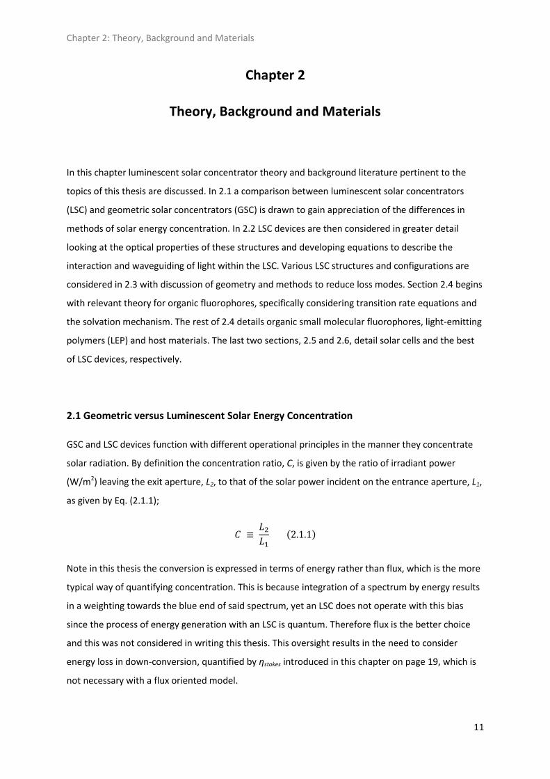
Considering the concentration ratio for lens based GSC devices, using Eq. (2.1.3), with the
assumption of θ2 = 90° and n = 1.5, the curve shown in Fig. 2.1.1 is plotted.
Figure 2.1.1: Concentration ratio for a GSC as a function of acceptance angle.
We see that CGSC only sharply increases below θ1 ≈ 20°, which is the regime where solar tracking will
be required. This can be seen from the relation between solid acceptance angle, Ω, and acceptance
angle, θ1, given by Ω = 2π(1 - cosθ1) Sr. A GSC for diffuse collection would need to have a solid
acceptance angle near Ω = 2π Sr but for θ1 = 20° we have Ω = 0.121π Sr. The highest point in Fig.
2.1.1, at the suns angular size of θ1 = 0.27°, is the maximum possible concentration that could be
achieved with a GSC with the given inputs. At CGSC ≈ 100000, typical practical applications for this
would be solar pumped lasers, destruction of hazardous wastes or powerful collimators.
Chapter 2: Theory, Background and Materials
14
LSC devices involve the coupling of solar irradiance to luminescent irradiance in a steady state
photophysical interaction. The irradiance at the output aperture is thus heavily dependent on the
spectral sensitivity of the fluorophore used, in absorption and emission. Geometry still plays an
important role in LSC devices with regards to the transmission of solar light into the device and the
coupling of the fluorophore irradiance to the LSC exit aperture, and hence the attached PV cells. It is
the transmission of solar light into the device that defines the ability of an LSC to collect diffuse
irradiance and this is governed by reflection at the interface (see Fig. 2.2.3). Determination of LSC
concentration ratio, CLSC, is more involved than for the treatment for GSCs here and is dealt with
through section 2.2, 2.3 and explored via the spectral analytical models of chapter 8.
LSC devices require no solar tracking because of the large acceptance angle, such tracking would add
excess expense for small gains and is therefore not a worthwhile investment. An additional benefit
of LSC devices over GSCs is that of thermal energy capture, which is exclusive to the concentrator
structure, where it is dissipated, whilst luminescent emission is delivered separately to the PV. This
means the PV does not suffer overheating problems, as it might under GSC concentration, and the
thermal energy could be extracted by coupling the LSC structure to a heat exchanger.
2.2 Loss Mechanisms in Luminescent Solar Concentrators
To understand how light moves into and propagates through the LSC structure an exploration of the
typical geometry and optical properties is necessary. In Fig 2.2.1 a LSC in simplest form is shown; it is
a planar rectangle made from some optical quality host material, with refractive index n, and doped
with small molecular fluorophores, at some concentration Cdye. Fig 2.2.1 shows various processes
that have influence over an LSC device's optical efficiency, ηopt, which is the fraction of incident light
concentrated at the exit aperture.
As shown in Fig. 2.2.1, incident solar radiation (1) impinges on the collecting face of the device and
due to Fresnel reflection a small part of that is reflected; about 4% at normal incidence (2). This of
course depends on angle of incidence and refractive index, as explored shortly. The remaining 96%
enters the device and the fluorescent dopants absorb this (3) and then re-emit it isotropically.
Because of Snell's laws of refraction a part of this subsequent emission is able to leave the device
without waveguiding (4), so called escape cone loss (ECL), but a larger part, around 75% as detailed
later, remains trapped due to total internal reflection (TIR). A large portion of the fluorescent
emission is then waveguided directly to the harvesting edge (5), where out-coupling is achieved, but
another portion becomes subject to self-absorption of fluorescence, due to the overlap in

Chapter 2: Theory, Background and Materials
15
absorption and emission spectra of the fluorescent species (6). Finally, because of the imperfect
absorption of the solar spectrum, there is a large portion of incident radiation which is transmitted
directly through the device without absorption (7).
Figure 2.2.1: Here is a schematic diagram of a basic square planar LSC device showing various mechanisms
which influence the resultant optical efficiency, ηopt. (1) incident light is either reflected (2) or enters the device
and is then either absorbed (3) or transmitted out the other side (7). Part of the trapped light is lost to the escape
cones (4) whilst the rest is waveguided through the structure until it either reaches the solar cell at the harvesting
edges or is self-absorbed (6) by members of the same luminescent species.
Other modes of loss not indicated in Fig 2.2.1 include transport related loss due to matrix scattering,
total internal reflection efficiency and a loss due to the quantum yield of the fluorophore. The
overall optical efficiency, ηopt, is given by the product of all the different loss modes quantified as
efficiencies, as in Eq. (2.2.1). Note that ηopt is defined here as a power efficiency, which is the
convention from older literature [3].
Where ηfr is the Fresnel efficiency due to reflection loss, ηtrap is the trapping efficiency due to angular
onset of TIR, ηTIR is the efficiency due to imperfections in the TIR interface, ηQY is the quantum yield
of the fluorophore, ηstokes is the efficiency due to down-conversion of absorbed energy, ηhost is the
efficiency of light transport through the host matrix, ηabs is the efficiency of absorption of incident
radiation and ηself is the efficiency due to self absorption. Each of these shall now be looked at
analytically to understand the parameter space they describe.
Fresnel efficiency for LSC devices, ηfr, is governed by the Fresnel equations for unpolarised light,
where the radiation is made up of equal mixture of p (parallel to surface) and s (perpendicular to
surface) polarisations. The reflection co-efficients, RS and Rp, for these two polarisations differ and
are given by Eqs. (2.2.2) and (2.2.3).
Chapter 2: Theory, Background and Materials
16
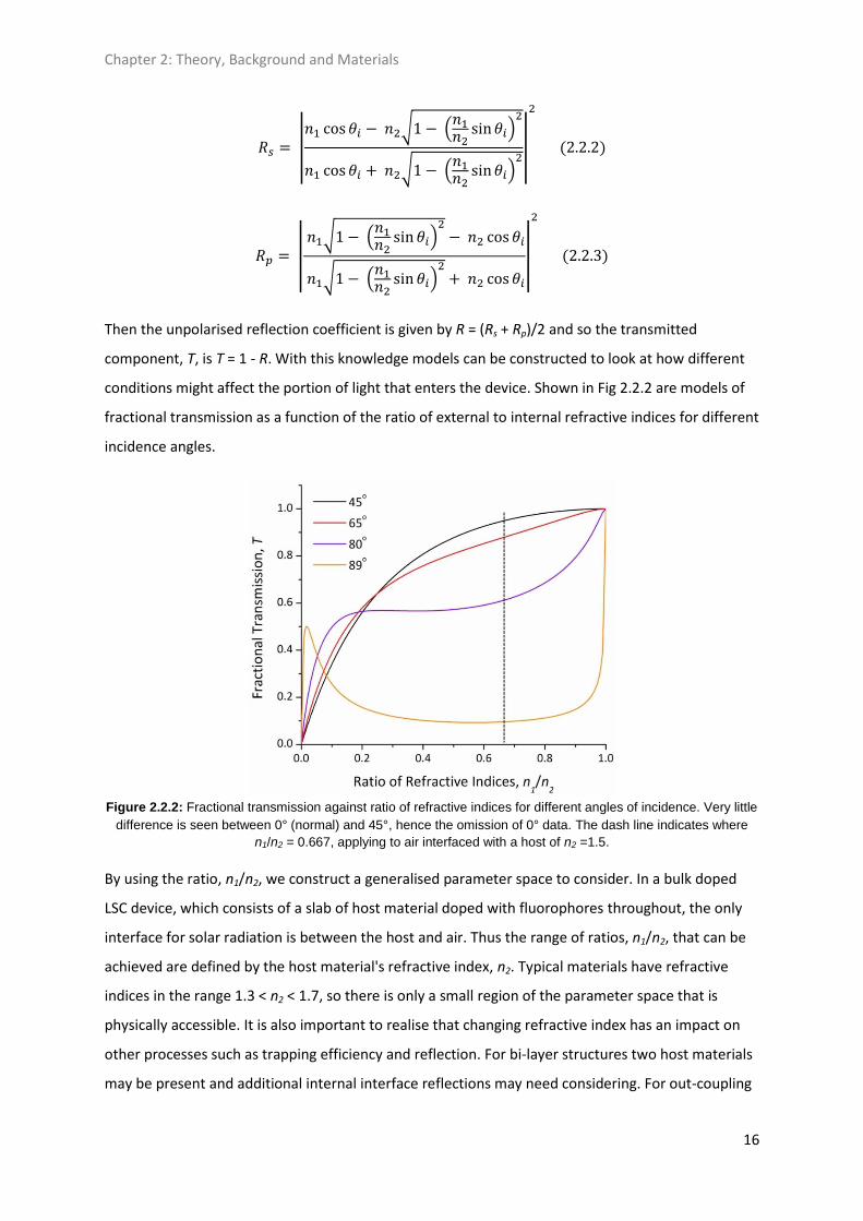
Then the unpolarised reflection coefficient is given by R = (Rs + Rp)/2 and so the transmitted
component, T, is T = 1 - R. With this knowledge models can be constructed to look at how different
conditions might affect the portion of light that enters the device. Shown in Fig 2.2.2 are models of
fractional transmission as a function of the ratio of external to internal refractive indices for different
incidence angles.
Figure 2.2.2: Fractional transmission against ratio of refractive indices for different angles of incidence. Very little
difference is seen between 0° (normal) and 45°, hence the omission of 0° data. The dash line indicates where
n1/n2 = 0.667, applying to air interfaced with a host of n2 =1.5.
By using the ratio, n1/n2, we construct a generalised parameter space to consider. In a bulk doped
LSC device, which consists of a slab of host material doped with fluorophores throughout, the only
interface for solar radiation is between the host and air. Thus the range of ratios, n1/n2, that can be
achieved are defined by the host material's refractive index, n2. Typical materials have refractive
indices in the range 1.3 < n2 < 1.7, so there is only a small region of the parameter space that is
physically accessible. It is also important to realise that changing refractive index has an impact on
other processes such as trapping efficiency and reflection. For bi-layer structures two host materials
may be present and additional internal interface reflections may need considering. For out-coupling

Chapter 2: Theory, Background and Materials
17
of waveguided fluorescence the reflections at the coupling interface, mediated by some coupling
material (e.g. silicone grease) to a solar cell, will also need to be considered. Fig 2.2.2 also shows us
that the reflected component does not significantly increase at n1/n2 = 0.667 until the incidence
angle is above around 45°. This is best seen by plotting T against θi as shown in Fig 2.2.3.
As Fig. 2.2.3 shows when we increase the host material's refractive index there is a small decrease in
transmission for normal incidence. For a typical host material good transmission acceptance is
expected to around θi = 65°, which corresponds to a solid acceptance angle of Ω = 1.155π Sr.
Remember a GSC can achieve Ω = 2π Sr for concentration ratios of C = 2.25 and n2 = 1.5. This was the
n2 limit of concentration. However, if LSC devices can be shown to achieve much higher C values
then the drop in transmission for higher incidence angles may be negated. To argue that LSC devices
are better suited to capture diffuse radiation this must be explored along with economic
considerations and it is therefore an aim of this thesis to do so (see chapter 8).
Figure 2.2.3: Fractional transmission against the angle of incidence for air interfaced to various host indices, n2.
After the radiation has entered the device it either gets absorbed by the fluorophores or transmits
straight through. Of the portion that is absorbed some is lost due to the fluorophore's quantum yield
but the rest is emitted. This emitted fraction now impinges on the internal interface with air and
depending on this angle of incidence of emission, θem, either undergoes TIR or refracts through the
interface and is lost via the ECL. This condition is derived via Snell's law and thus quantified by the
trapping efficiency, ηtrap, given by Eq. (2.2.4) [4].
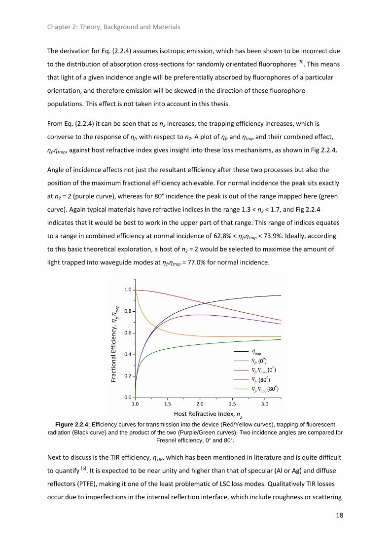
Chapter 2: Theory, Background and Materials
18
The derivation for Eq. (2.2.4) assumes isotropic emission, which has been shown to be incorrect due
to the distribution of absorption cross-sections for randomly orientated fluorophores [5]. This means
that light of a given incidence angle will be preferentially absorbed by fluorophores of a particular
orientation, and therefore emission will be skewed in the direction of these fluorophore
populations. This effect is not taken into account in this thesis.
From Eq. (2.2.4) it can be seen that as n2 increases, the trapping efficiency increases, which is
converse to the response of ηfr with respect to n2. A plot of ηfr and ηtrap and their combined effect,
ηfrηtrap, against host refractive index gives insight into these loss mechanisms, as shown in Fig 2.2.4.
Angle of incidence affects not just the resultant efficiency after these two processes but also the
position of the maximum fractional efficiency achievable. For normal incidence the peak sits exactly
at n2 = 2 (purple curve), whereas for 80° incidence the peak is out of the range mapped here (green
curve). Again typical materials have refractive indices in the range 1.3 < n2 < 1.7, and Fig 2.2.4
indicates that it would be best to work in the upper part of that range. This range of indices equates
to a range in combined efficiency at normal incidence of 62.8% < ηfrηtrap < 73.9%. Ideally, according
to this basic theoretical exploration, a host of n2 = 2 would be selected to maximise the amount of
light trapped into waveguide modes at ηfrηtrap = 77.0% for normal incidence.
Figure 2.2.4: Efficiency curves for transmission into the device (Red/Yellow curves), trapping of fluorescent
radiation (Black curve) and the product of the two (Purple/Green curves). Two incidence angles are compared for
Fresnel efficiency, 0° and 80°.
Next to discuss is the TIR efficiency, ηTIR, which has been mentioned in literature and is quite difficult
to quantify [6]. It is expected to be near unity and higher than that of specular (Al or Ag) and diffuse
reflectors (PTFE), making it one of the least problematic of LSC loss modes. Qualitatively TIR losses
occur due to imperfections in the internal reflection interface, which include roughness or scattering
Chapter 2: Theory, Background and Materials
19
due to grain formation or dirt collecting on the outer surface. Other factors include the employment
of mirrors; an air gap should always be used as thermally evaporated mirrors will reduce TIR
efficiency, because the mirror has a lower reflection efficiency than the host/air interface, and will
also lead to further roughening of said interface [7]. Clearly the fabrication process is critical for
maximising the TIR efficiency and polishing of the collection face could help reduce this loss mode.
The concentrator surface will suffer from the build up of dirt highlighting the need to clean and
polish the collection face over time.
The fluorescence quantum yield, ηQY, is a key factor which describes the emission efficiency of the
fluorophores employed. This encompasses all of the electronic process that affect emission including
all radiative and non-radiative recombination pathways. This will be discussed further in section 2.4,
but bear in mind here that it has a strong influence over the amount of light being put into
waveguided modes. Because of this it also has a strong relationship with the self-absorption loss
mode and subsequent orders of emission.
Arguably the Stokes' efficiency, ηstokes, doesn't represent a real loss because the loss of energy in
down-conversion at the fluorophore is similar to that occurring at the band-gap of a solar cell under
direct illumination. Considering that exciton generation is quantum, and so a single photon gives rise
to a single exciton, it does not make sense to think of this as a loss. ηstokes was quantified in 1981 to
have a foreseeable maximum of ηstokes = 0.75 [3], which is the value used throughout this thesis.
Ultimately it comes down to the choice between energy (wavelength) or flux in the quantification of
irradiance, as discussed at the start of section 2.1, and since this thesis uses energy the value ηstokes =
0.75 must be used. Many researchers include this as a loss mode [3,6,8] because of the choice of
energy over flux in their models. However, work in the literature has shown that with the correct
choice of solar cell, coupling favourably to the fluorescence radiation field, up to a 20% relative
increase in power conversion can be expected [9]. This highlights again that using flux to quantify
irradiance is the better choice.
In terms of light transport the host material itself will absorb some energy across the visible
spectrum and convert this to heat. Additionally imperfections in the host matrix can cause scattering
of light, quantified through the host efficiency, ηhost, which can be estimated by measuring the
optical absorption of undoped sample plates. The number of defects present in the host matrix can
be affected by the formation process and the presence of dopants [10] and there is evidence that
matrix losses may comprise a major loss mode. This has been shown experimentally by
measurement of flux output in the presence and absence of a reflector at the opposite LSC edge to
that measured [11]. One would expect a factor of 2 increase in output in this case, which was not
Chapter 2: Theory, Background and Materials
20
seen. ηhost has been estimated to have a value between 0.95-0.98 for a PMMA host transporting light
in the visible region [12]. Furthermore the properties of the matrix have a significant bearing on the
dopant fluorophore in terms of the emission wavelength, quantum yield and lifetime stability (see
chapter 7). Given these factors not only is the choice of host material critical, but also how the LSC
device is manufactured. This thesis cannot cover the materials science of polymerisation processes
in different fabrication and deposition methods, but it is worth taking into account that this
engineering is necessary for a high quality LSC. The best polymers to date are made from the
materials used for efficient optical fibres such as poly(methyl methacrylate) (PMMA), which has an
optical absorption of 3.5x10⁻⁴ cm-1 and n = 1.494 at λ = 550nm [13]. Ideally a host of higher index and
similar optical absorption would be chosen. Additional absorption may be present from defects.
To quantify ηhost, the absorption coefficient, αh(λ), of the host medium must be measured and then
the mean path length of waveguide modes determined. αh(λ) is determined through Beer-Lambert
law;
Where I(λ) is the intensity after passing through an absorption path length, l, of a medium of
absorption coefficient, αh(λ), with initial incident intensity, I0(λ). For the host matrix the attenuation
coefficient αh(λ), with units cm-1, is sufficient but for absorption by fluorophores at some
concentration, Cdye [M], then we use αd(λ) = εd(λ)Cdye where εd(λ) is the molar absorptivity, or
extinction coefficient, with units M-1cm-1. Experimentally it is quite challenging to measure αh(λ) for
materials like PMMA because it is so low one needs a large thickness to make measurements. This
means fabricated plates of material are required instead of thin films made easily in the lab. From
Eq. (2.2.5) we can quantify the matrix losses as the ratio of final and initial intensities over the mean
path length of waveguide modes traversing a host medium of averaged absorption coefficient <α>;
This is an approximation and may be a best estimate since αh(λ) is measured in the absence of
dopants. In literature matrix related losses have received some attention; in 1981 the combined
effect of ηTIR and ηhost was quantified experimentally as 0.9, with 0.95 expected in the future [11]. As
stated above with ηTIR expected to be near unity and with 0.95 < ηhost < 0.98 this is likely to be higher
in an optimised device. This will depend on the geometry of the LSC device, and hence path length of
light through it, which is an area that requires some thought with a view to optimisation.
Chapter 2: Theory, Background and Materials
21
Much more can be done using the Beer-Lambert law of Eq. (2.2.5). The absorption efficiency, ηabs, is
determined by the ratio of the integral of collected irradiance spectrum, S0(λ), to that of the solar
irradiance spectrum, Ssun(λ). By determining εd(λ) for a given fluorophore, the absorption of solar
energy as a function of depth and dye concentration can be explored. Going further, a multi-dye
plate or stack of plates may be considered and it is therefore possible to think about what values for
ηabs are possible from different LSC device configurations. Additionally if a Förster Resonant Energy
Transfer (FRET - see Section 2.4) system of multiple fluorophores were to be employed then Eq.
(2.2.5) could be used to model how that system collects incident sunlight. Then, by knowing the
quantum efficiencies, FRET efficiencies and the normalised emission spectra, the fluorescence
output, S1(λ), of the terminal dye can easily be predicted.
For the simple case of a single fluorophore device of quantum yield ηQY, εd(λ) is measured
experimentally and then S0(λ) is determined via Eq. (2.2.5) with I0(λ) = Ssun(λ), l as the path length
through the LSC and αd(λ) = εd(λ)Cdye for the fluorophore. Now the first order fluorescence output,
S1(λ), is given by equating the quantum yield corrected total absorbed energy to the total emitted
energy as in Eq. (2.2.7);
S1(λ) is the goal, which is related to the normalised emission spectrum, SN(λ), from fluorescence
spectroscopy on the fluorophore at the required dye concentration, Cdye, via some maximum
intensity, Imax, which we do not know;
Note that SN(λ) is the fundamental emission spectrum prior to any effect which changes the line-
shape, such as self-absorption. Substituting Eq. (2.2.8) into Eq. (2.2.7) allows us to determine Imax;
This is the scaling factor with which to scale SN(λ) by to achieve a quantum yield corrected equivalent
intensity fluorescence output using Eq. (2.2.8). One must also consider the escape cone loss for the
true, captured output and so the waveguided irradiance spectrum is given by Eq. (2.2.10);

Chapter 2: Theory, Background and Materials
22
By knowing the intensity of the fluorescence it is possible to then go on and inform the coupling with
the solar cell external quantum efficiency spectrum, ηEQE(λ,θ), at the harvesting face. ηEQE(λ,θ) is the
ratio of electron hole pairs collected at the interface to the number of incident photons and is a
function of both wavelength and incidence angle. Since the angle is typically considered to be
normal this is often expressed as just ηEQE(λ).
Eq. (2.2.5) can also be used to describe the change in the fluorescence intensity, as a function of
wavelength, with distance through the LSC medium due to the self-absorption process, ηself. ηself is
another parameter that is difficult to measure absolutely and is a function of fluorophore
concentration, Cdye, and mean fluorescence path length, <r>. It may have a more complex spatial
dependence due to local variations in dye concentration or for bi-layer device structures. Many
fluorescent materials exhibit an overlap in their absorption and emission spectra, which means
emission in that overlap region may be reabsorbed by other same species dye molecules. This
reabsorbed light has a chance of being re-emitted, ηQY, and after emission there is a chance of TIR
into waveguide modes related to ηtrap. We also need to consider that this new generation of
emission will be subject to matrix and TIR efficiency losses, ηhost and ηTIR. Of course there could be a
third generation reabsorption and emission and so on, with each subsequent generation being lower
in population than the previous one.
The actual strength of the self-absorption is wavelength dependant but can be estimated in simplest
form by the overlap integral, J, as a fraction of the integral of the emission spectrum of a given
order, i.e. ηself = (1-J). Now Eq. (2.2.1) can be expanded to encompass all generations. Note that for
higher generations of emission the self-absorption strength, J, is an extra factor;
Summation over all generations gives the final optical efficiency;
In practice it can be seen that generations of fluorescence above p = 3 have a negligible contribution
to the optical efficiency. Contributions for p = 3 are typically less than 0.2% of the total and for p > 3
this becomes less than 0.01% with exact values depending on the particular fluorophore (i.e. the size
of J). However, because this equation does not take into account the mean path length of light in the
waveguide it is not valid for particular LSC geometries. Since the overlap integral is a first guess
estimator for ηself this equation is used only to compare optical efficiencies in a relative manner, as in
Chapter 5.
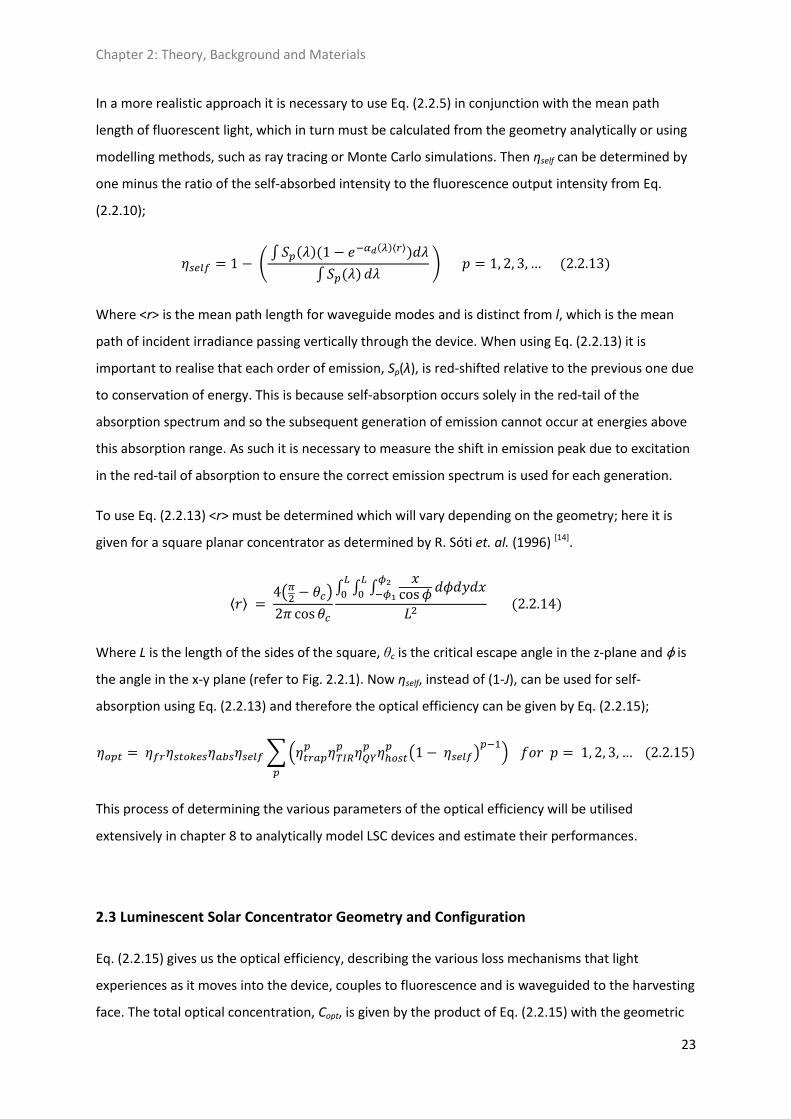
Chapter 2: Theory, Background and Materials
23
In a more realistic approach it is necessary to use Eq. (2.2.5) in conjunction with the mean path
length of fluorescent light, which in turn must be calculated from the geometry analytically or using
modelling methods, such as ray tracing or Monte Carlo simulations. Then ηself can be determined by
one minus the ratio of the self-absorbed intensity to the fluorescence output intensity from Eq.
(2.2.10);
Where <r> is the mean path length for waveguide modes and is distinct from l, which is the mean
path of incident irradiance passing vertically through the device. When using Eq. (2.2.13) it is
important to realise that each order of emission, Sp(λ), is red-shifted relative to the previous one due
to conservation of energy. This is because self-absorption occurs solely in the red-tail of the
absorption spectrum and so the subsequent generation of emission cannot occur at energies above
this absorption range. As such it is necessary to measure the shift in emission peak due to excitation
in the red-tail of absorption to ensure the correct emission spectrum is used for each generation.
To use Eq. (2.2.13) <r> must be determined which will vary depending on the geometry; here it is
given for a square planar concentrator as determined by R. Sóti et. al. (1996) [14].
Where L is the length of the sides of the square, θc is the critical escape angle in the z-plane and φ is
the angle in the x-y plane (refer to Fig. 2.2.1). Now ηself, instead of (1-J), can be used for self-
absorption using Eq. (2.2.13) and therefore the optical efficiency can be given by Eq. (2.2.15);
This process of determining the various parameters of the optical efficiency will be utilised
extensively in chapter 8 to analytically model LSC devices and estimate their performances.
2.3 Luminescent Solar Concentrator Geometry and Configuration
Eq. (2.2.15) gives us the optical efficiency, describing the various loss mechanisms that light
experiences as it moves into the device, couples to fluorescence and is waveguided to the harvesting
face. The total optical concentration, Copt, is given by the product of Eq. (2.2.15) with the geometric

Chapter 2: Theory, Background and Materials
24
concentration, G. The geometric concentration is given by the ratio of the areas of the collection
face to the harvesting faces as in Eq. (2.3.1);
So then the optical concentration is given by Eq. (2.3.2);
In addition to optimising all of the factors that ηopt is comprised of it is also necessary to mutually
optimise the geometry of the LSC device to maximise G. There are two main geometries for LSC
devices, square-planar and cylindrical, though triangular designs using mirrors have been suggested
for their low mean path lengths and hence lower matrix and self absorption losses [4]. Technically
this is a planar arrangement anyway and a number of other planar arrangements, such as hexagonal,
have been looked at [14]. In that work the path length is shown to be approximately equal to the
square root of the LSC surface area, which increases with the number of sides the LSC has, and
hence to minimise self-absorption an equilateral triangle should perform best in terms of optical
efficiency. For square-planar devices the geometric concentration, Gsq, for a square plate of side
lengths L and thickness W is given by Eq. (2.3.3);
Similarly the geometric concentration for a cylindrical LSC, Gcyl, of length L and radius R is given by;
By relating R and W, as R =2W/π, it has been shown that the relationship between the geometric
concentration for a square-planar LSC to that of a cylindrical LSC is as in Eq. (2.3.5) [15];
Cylindrical LSC geometries can thus potentially achieve double the geometric concentration of a
square-planar LSC structure. This benefit is offset by typically longer path lengths and greater Fresnel
reflection at the interface. However, the K. R. McIntosh et. al. 2007 paper sets the stage for bi-layer
LSC device structures as it shows, through geometric arguments, that the cylindrical geometry could
outperform square ones by as much as a factor of 1.9 if the fluorescence occurs near the surface. In
this regime, for a coated cylinder, a more optically dense medium is necessary to maximise
absorption (hence a higher fluorophore concentration). Additional small increases in performance
Chapter 2: Theory, Background and Materials
25
and a reduction of the Fresnel loss, beating that of square-planar geometry, are possible using a
multi-cylindrical design, like a corrugated surface. It has been seen in Fig. 2.2.4, for normal incidence,
that ηfr = 0.96 for a square-planar device of n2 = 1.5; for a single cylinder this becomes ηfr = 0.931 and
for a multi-cylindrical LSC we have ηfr = 0.973. This shows that a multi-cylindrical LSC structure would
reflect less light than a planar geometry LSC at normal incidence. Note also that for diffuse light at
smaller angles of incidence K. R. McIntosh et. al. 2007 show that cylindrical geometries would
outperform the square planar geometry in terms of ηfr, lending cylindrical LSC devices to be better
for cloudy, northern climes. Therefore a multi-cylindrical design would outperform a planar
geometry for both direct and diffuse solar irradiance.
Other potential benefits of the cylindrical approach include ease of affixing a PV cell to the
harvesting edge of the device and the higher G values meaning smaller PV cells are needed and
hence potentially lower cost. One of the main downsides one might expect of the cylindrical
approach is due to the larger mean path length through the device, resulting in higher matrix and
self-absorption losses. These could be quantified analytically using Eq. (2.2.6) and Eq. (2.2.13) for a
deeper comparison of the geometries, which has been done using more advanced Monte Carlo
simulation methods [16]. In that work self-absorption is shown to peak for short cylindrical LSC
lengths, particularly for coated fibre LSCs where emission close to the surface results in a higher
fraction of long, helical paths through the more optically dense outer medium. Despite this the
authors show that even after self-absorption peaks the optical concentration continues to rise with
increasing cylinder length, unlike with square-planar geometries where self-absorption results in the
optical concentration reaching a plateau value. Thus a cylinder can benefit from a longer length, L,
than a square-planar LSC.
From the above discussion of geometry follows the realisation that bi-layer structures may offer an
advantage over conventional bulk-doped designs for the cylindrical geometry. K. R. McIntosh et. al.
2007 seems to imply, by omission, that surface emission for square-planar devices offers no benefit
over bulk-doping. This was shown rigorously by R. Bose et. al. 2007 through experimental devices
and ray-tracing models [17].
The configuration of an LSC device includes more aspects than geometric shape. Other factors
include the employment of mirrors [11] and wavelength selective filters [18 - 21], multi-stack (tandem)
plates [3, 19, 22], multi-dye plates [23], anti-reflection coatings [4], plasmonic enhancements [5, 8, 24], and
the use of lenses [25]. These factors are with an aim to maximising ηfr, ηtrap, ηQY, ηabs, ηself and ηhost and
minimising the total cost of the device. Let's go over each of these efficiencies in some detail to see
Chapter 2: Theory, Background and Materials
26
how different configuration factors can be used to improve the loss mechanisms these efficiencies
represent.
The reflection of incident sunlight, governed by ηfr, represents a relatively small loss which
nonetheless needs optimising. The way to improve this is to use an antireflection coating, such as
MgF2, which works by having a much higher refractive index. Such materials are unsuited to being
hosts, but a thin layer on the LSC collection face can have very high transparencies and could provide
a relative improvement of transmission efficiency by around 3% [4]. This figure actually depends on
the incidence angle, with normal incidence exhibiting the lowest benefits from the coating.
Additionally, as seen in the geometry discussion, a multi-cylindrical LSC actually has an advantage in
this loss mode over square and single cylindrical designs.
There are two main ways that have been suggested to improve the trapping efficiency, ηtrap, which
represents a major loss of around 25% for n2 = 1.5 according to Eq. (2.2.4). Additionally self-
absorption results in further ECL, compounding the problem, particularly for fluorophores with a
large overlap integral, J. Since ηtrap depends only on the refractive index of the host it would seem all
that can be done is to change the host matrix, as explored in Fig (2.2.4). However, it is possible to
use frequency selective filters to reflect emission wavelengths, but allow incident solar irradiance in
the fluorophore absorption regime [11, 18, 19]. These filters are photonic structures and can be made
from crystalline materials, such as diamond, ceramics or tantalum oxide, Ta2O5, which are formed to
have a periodically varying refractive index. This creates stop band regions of disallowed energies
which display high reflectivity for photons of those energies and can be tuned to encompass desired
ranges. Hence these filters are called wavelength selective mirrors and such structures are known as
Distributed Bragg Reflectors (DBR). Other materials include cholesteric coatings, a type of organic
liquid crystal that form a helical 3D structure which reflects circularly polarised light aligned with the
structure [20]. These have already been shown to reduce the light lost in the escape cone by up to
30% [21]. It has been shown by Monte Carlo ray tracing simulations that the upper limit of efficiency
for a LSC is equal to the Shockley-Queisser (SQ) limit for solar cells [18]. It is concluded that to reach
the thermodynamic limit of concentration with LSC devices wavelength selective mirrors will be
required.
A final possibility to enhance ηtrap is to align dyes vertically, as opposed to randomly, which will
deviate the emission from isotropic to increase photon populations in waveguide modes [26]. A
downside to this is a reduction in the absorption cross-section of the dyes relative to normally
incident solar irradiance, increasing the required LSC thickness or fluorophore concentration.
However, this is for normal incidence; as the sun moves across the sky, and for diffuse light from
Chapter 2: Theory, Background and Materials
27
clouds, this should not necessarily be a limitation. One would need to optimise the fluorophore
alignment angle alongside the absorption efficiency across a day, for local sky conditions, to achieve
the best results.
The fluorescence quantum yield, ηQY, of fluorophores in an LSC device is required to be near unity,
which imposes strict limitations on their properties. Fluorophores must exhibit near unity quantum
yield in a solid state host matrix at concentrations that enable maximisation of absorption efficiency,
ηabs, discussed in detail next. The concentration quenching phenomenon is a major problem in this
context (see chapter 7) and careful tuning of both fluorophore concentration and LSC absorption
path length are necessary to maximise LSC irradiant output. ηQY can be effectively enhanced by
plasmonic resonance, which has been shown to increase the absorption and fluorescence transition
rates and thus can increase LSC output irradiance [24]. In that work CdSe/ZnS quantum dot
fluorophores are coupled to surface plasmons generated on various concentrations of gold
nanoparticles, providing up to 53% increase in emission. Work by Zhang et. al. (2007) [27] exhibited
an enhancement in fluorescence of up to 100% for a perylene based dye deposited on a glass
substrate coated with Ag plasmons. As well as enabling enhancement of fluorophore absorption and
emission plasmonic resonance has been shown to increase solar cell absorption, and hence quantum
efficiency, allowing more energy to be collected in an LSC device [28].
Possibly the biggest issue with LSC devices is in attempting to maximise the amount of solar energy
captured, as quantified by ηabs. Firstly there is an absorption limit due to the range that can be
covered by the spectral sensitivity of the solar cell coupled to the LSC. The absorption spectrum of
the fluorophore/s needs to cover the entire range of energies up to the solar cell band edge and the
emission spectrum needs to overlap strongly with the absorption band of the cell. The bigger
challenge is to design a system to maximise absorption of the possible range of solar energies and
there are several proposed ways of doing this.
Firstly the thickness (or radius) of the LSC device is optimised using Eq. (2.2.5), as outlined in the
relevant section above. However it is a necessary to add a factor to this thickness optimisation; that
being employment of mirrors. It might be wasteful in terms of geometric concentration, and hence
solar cell size, to increase the plate thickness too much and so adding an inexpensive mirror or
diffuse reflector to the back side of the device can alleviate this [11, 29]. The reflector will give incident
light a second pass through the LSC device and hence improve the absorption considerably, whilst
allowing optimisation of G at the same time. This is explored by spectral models in chapter 8.
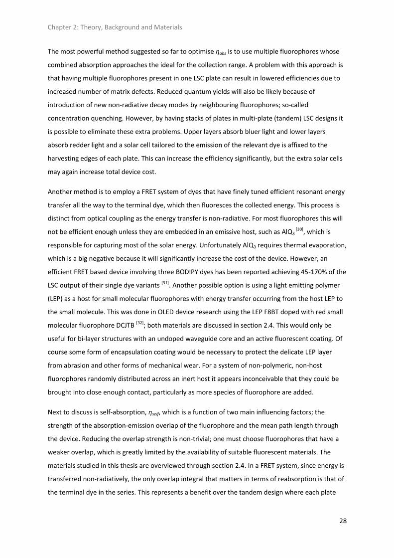
Chapter 2: Theory, Background and Materials
28
The most powerful method suggested so far to optimise ηabs is to use multiple fluorophores whose
combined absorption approaches the ideal for the collection range. A problem with this approach is
that having multiple fluorophores present in one LSC plate can result in lowered efficiencies due to
increased number of matrix defects. Reduced quantum yields will also be likely because of
introduction of new non-radiative decay modes by neighbouring fluorophores; so-called
concentration quenching. However, by having stacks of plates in multi-plate (tandem) LSC designs it
is possible to eliminate these extra problems. Upper layers absorb bluer light and lower layers
absorb redder light and a solar cell tailored to the emission of the relevant dye is affixed to the
harvesting edges of each plate. This can increase the efficiency significantly, but the extra solar cells
may again increase total device cost.
Another method is to employ a FRET system of dyes that have finely tuned efficient resonant energy
transfer all the way to the terminal dye, which then fluoresces the collected energy. This process is
distinct from optical coupling as the energy transfer is non-radiative. For most fluorophores this will
not be efficient enough unless they are embedded in an emissive host, such as AlQ3 [30], which is
responsible for capturing most of the solar energy. Unfortunately AlQ3 requires thermal evaporation,
which is a big negative because it will significantly increase the cost of the device. However, an
efficient FRET based device involving three BODIPY dyes has been reported achieving 45-170% of the
LSC output of their single dye variants [31]. Another possible option is using a light emitting polymer
(LEP) as a host for small molecular fluorophores with energy transfer occurring from the host LEP to
the small molecule. This was done in OLED device research using the LEP F8BT doped with red small
molecular fluorophore DCJTB [32]; both materials are discussed in section 2.4. This would only be
useful for bi-layer structures with an undoped waveguide core and an active fluorescent coating. Of
course some form of encapsulation coating would be necessary to protect the delicate LEP layer
from abrasion and other forms of mechanical wear. For a system of non-polymeric, non-host
fluorophores randomly distributed across an inert host it appears inconceivable that they could be
brought into close enough contact, particularly as more species of fluorophore are added.
Next to discuss is self-absorption, ηself, which is a function of two main influencing factors; the
strength of the absorption-emission overlap of the fluorophore and the mean path length through
the device. Reducing the overlap strength is non-trivial; one must choose fluorophores that have a
weaker overlap, which is greatly limited by the availability of suitable fluorescent materials. The
materials studied in this thesis are overviewed through section 2.4. In a FRET system, since energy is
transferred non-radiatively, the only overlap integral that matters in terms of reabsorption is that of
the terminal dye in the series. This represents a benefit over the tandem design where each plate
Chapter 2: Theory, Background and Materials
29
has a distinct fluorophore with its own overlap integral to reduce efficiency by. Another method that
may prove useful, particularly in tandem designs, is to use the solvation mechanism to increase the
dyes Stokes' Shift, ΔEstokes. This only works for polar fluorophores whose dipole moment changes
upon excitation to the S1 state and is facilitated by increasing the relative permittivity, εr, of the host
medium. This mechanism is explored in greater detail in section 2.4 and chapter 6. The other way to
increase ηself is by reduction of the mean path length by various means including choice of geometry,
optimisation of G and aligning dyes to emit into shorter waveguide modes [26].
The light transport efficiency of the host, ηhost, is governed by the type of host material, fabrication
methods (defects), the presence of unreacted monomer or additives, the fluorophore concentration
and type, and the path length of light. Typical polymeric host materials exhibit strong absorption at
around 750 nm, due to vibrational modes of C-H bonds, resulting in luminescence quenching due to
non-radiative energy transfer of the vibrational energy [33]. This could be improved by substitution of
hydrogen for deuterium or fluorine atoms to reduce bond vibration [34]. An alternative would be to
use a specialist glass, which reportedly could deliver better transport properties and higher
refractive indexes but has the downside of being heavy and more expensive [35].
Host fabrication method is also a critical issue; polymerisation from precursor and monomer
components is of low cost but can result in unreacted monomers disrupting the matrix [6]. Another
issue is the lack of control over the molecular weight, MW, and regioregularity of the polymerised
host. The conditions of the polymerisation such as temperature, solvent and time all affect the
resultant matrix and its properties thus requiring careful tuning of the polymerisation process to
achieve the optimal matrix. Another approach is casting from solution with pre-polymerised and
purified host materials, which is of low cost and simple but may result in the presence of unwanted
solvent residue. Again formation processes are critical including drying time, solvent, temperature
and so on. A main benefit of this approach is control of the molecular weight of the host material,
which may be crucial for matrix stability over device lifetime. Stability is used here as a general term,
being the resistance of the matrix to environmental damage such as from thermal stresses,
photodegradation and interactions with oxygen. Most monomers, such as MMA or styrene, are
liquids so need to have some level of polymerisation to be solid at room temperature. Further, in the
literature it has been shown for PMMA that fracture energy, y, is proportional to the square of
molecular weight (y MW2), up to a critical value of MW at which y is constant [36]. A strong PMMA
structure should therefore have a high MW, but there are other factors that may need consideration
such as MW impacts on ηQY, as briefly explored in chapter 7. Another approach altogether employs
sol-gel methods for glass forming, which are widely used and could result in improved LSC yields [37].
Chapter 2: Theory, Background and Materials
30
Such a large range of potential solutions to the innate complexity of trying to optimise LSC devices as
a whole presents a mammoth challenge for technology developers. The developments necessary for
LSCs to reach a commercial application, with an optical efficiency of ηopt > 10%, can be broken down
into six main criteria:
1. Broad absorption range
2. Minimum overlap of absorption and emission spectra
3. High quantum yield, ηQY, (modern organic dyes and rare earth materials have ηQY > 90%)
4. Low matrix attenuation
5. Lifetime in excess of ten years (Si-cells have 20 year lifetimes)
6. Competitive device cost (< 1 $/W)
Because of the sheer number of loss modes and their possible solutions, optimisation by empirical
methods is an incredibly complex and daunting task. Therefore it is good idea to take a modelling
approach to inform the optimisation process and reduce the vast number of permutations that need
exploring [3, 38-40]. Thermodynamics provides the maximum limits possible. Equations governing
geometrical optics, as discussed earlier, are used to compare different geometries and to
understand the importance of the optical properties of the host. Monte Carlo and ray tracing
methods are typically employed to explore the movement of light and how introduction of
configuration factors, such as PBS filters, can influence this. Such work is critically informative to the
experimental research process.
2.4 Semiconductor Physics for LSC Devices and Materials
Various fluorophore materials are under consideration for LSC devices including organic dyes [41, 42],
inorganic nanocrystals [43-45] and rare earth materials [46-48]. The underlying physical processes that
govern these materials are essentially the same, involving the quantum mechanics of transitions,
albeit with varying degrees of complication. In this thesis organic dye systems are the focus and the
following discussion relates to these in particular.
LSC devices rely on photoexcitation of the fluorophores and therefore typically involve allowed,
asymmetric quantum mechanical transitions, giving rise to photoluminescence (PL). There are some
major deviations from this for particular materials, so called phosphors, which exhibit strong spin-
orbit coupling resulting in high intersystem crossing rates and hence the triplet emission form of PL.
Chapter 2: Theory, Background and Materials
31
Such materials are typically organometallic compounds with a metal atom, such as Iridium or
Europium, as a core structure.
In photon absorption an electron in the ground state is promoted to a higher energy state of the
fluorophore. The absorption process allows for any ground state (S0) electron to be excited to a
higher energy level, so long as the photon has the energy to do so. Because of vibrational modes
coupling with the principal quantum states, each energy level is actually a manifold of states
resulting in observed broadening of the spectrum. These coupled vibronic states are often called
vibronic satellites. This can be seen by considering a configuration diagram, which represents the
potentials of each energy level and the associated coupled vibronic structure, as shown in Fig 2.4.1.
Figure 2.4.1: Configuration diagram showing transitions between the S0 and S1 excited states. Each transition
mode has a particular probability of occurrence depending on the wavefunction overlap in vertical transitions.
Note the different energies of absorption (A) and fluorescence (F) due to energy lost to nuclear vibrations in
excited state relaxation. This explains the Stokes' shift, ΔEstokes.
The nature of these vibronic states arises from oscillations in the nucleus and is described by the
Franck-Condon Principle [49], which also gives an explanation for ΔEstokes. The nucleus responds very
slowly relative to the absorption process, which takes roughly a femtosecond, and is therefore
essentially static. However, the excited state exists for around a nanosecond during which time the
nucleus starts to oscillate like a spring due to the new electronic configuration putting the nucleus in
a non-equilibrium position. The nucleus can oscillate many thousands of times in the lifetime of the
excited state over which most if not all of this vibrational energy is transferred to the surrounding
medium as heat, a process called Internal Conversion (IC). Then fluorescence takes place from the
lowest vibrational state of the electronic manifold of the S1 excited state.
The Frank-Condon Principle is best exhibited though the absorption and emission spectrum of a
simple organic fluorophore, such as perylene, since such molecules have strong vibrational coupling.
More complex and flexible organic molecules tend to have absorption and emission dominated by a
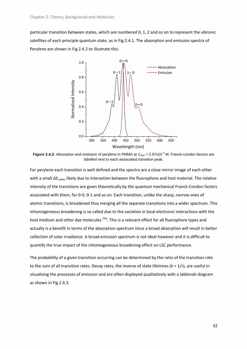
Chapter 2: Theory, Background and Materials
32
particular transition between states, which are numbered 0, 1, 2 and so on to represent the vibronic
satellites of each principle quantum state, as in Fig 2.4.1. The absorption and emission spectra of
Perylene are shown in Fig 2.4.2 to illustrate this.
Figure 2.4.2: Absorption and emission of perylene in PMMA at Cdye = 2.97x10⁻³
M. Franck-condon factors are
labelled next to each associated transition peak.
For perylene each transition is well defined and the spectra are a close mirror image of each other
with a small ΔEstokes likely due to interaction between the fluorophore and host material. The relative
intensity of the transitions are given theoretically by the quantum mechanical Franck-Condon factors
associated with them, for 0-0, 0-1 and so on. Each transition, unlike the sharp, narrow ones of
atomic transitions, is broadened thus merging all the separate transitions into a wider spectrum. This
inhomogeneous broadening is so called due to the variation in local electronic interactions with the
host medium and other dye molecules [50]. This is a relevant effect for all fluorophore types and
actually is a benefit in terms of the absorption spectrum since a broad absorption will result in better
collection of solar irradiance. A broad emission spectrum is not ideal however and it is difficult to
quantify the true impact of the inhomogeneous broadening effect on LSC performance.
The probability of a given transition occurring can be determined by the ratio of the transition rate
to the sum of all transition rates. Decay rates, the inverse of state lifetimes (k = 1/τ), are useful in
visualising the processes of emission and are often displayed qualitatively with a Jablonski diagram
as shown in Fig 2.4.3.
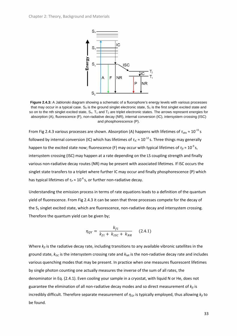
Chapter 2: Theory, Background and Materials
33
Figure 2.4.3: A Jablonski diagram showing a schematic of a fluorophore's energy levels with various processes
that may occur in a typical case. S0 is the ground singlet electronic state, S1 is the first singlet excited state and
so on to the nth singlet excited state, Sn. T1 and T2 are triplet electronic states. The arrows represent energies for
absorption (A), fluorescence (F), non-radiative decay (NR), internal conversion (IC), intersystem crossing (ISC)
and phosphorescence (P).
From Fig 2.4.3 various processes are shown. Absorption (A) happens with lifetimes of τabs ≈ 10-15 s
followed by internal conversion (IC) which has lifetimes of τIC ≈ 10-12 s. Three things may generally
happen to the excited state now; fluorescence (F) may occur with typical lifetimes of τfl ≈ 10-9 s,
intersystem crossing (ISC) may happen at a rate depending on the LS coupling strength and finally
various non-radiative decay routes (NR) may be present with associated lifetimes. If ISC occurs the
singlet state transfers to a triplet where further IC may occur and finally phosphorescence (P) which
has typical lifetimes of τP ≈ 10-6 s, or further non-radiative decay.
Understanding the emission process in terms of rate equations leads to a definition of the quantum
yield of fluorescence. From Fig 2.4.3 it can be seen that three processes compete for the decay of
the S1 singlet excited state, which are fluorescence, non-radiative decay and intersystem crossing.
Therefore the quantum yield can be given by;
Where kfl is the radiative decay rate, including transitions to any available vibronic satellites in the
ground state, kISC is the intersystem crossing rate and kNR is the non-radiative decay rate and includes
various quenching modes that may be present. In practice when one measures fluorescent lifetimes
by single photon counting one actually measures the inverse of the sum of all rates, the
denominator in Eq. (2.4.1). Even cooling your sample in a cryostat, with liquid N or He, does not
guarantee the elimination of all non-radiative decay modes and so direct measurement of kfl is
incredibly difficult. Therefore separate measurement of ηQY is typically employed, thus allowing kfl to
be found.

Chapter 2: Theory, Background and Materials
34
To maximise fluorescence ηQY, fluorophores for LSC devices are therefore to be chosen on the
condition of negligible kISC and kNR. Non-radiative decay may take the form of intrinsic non-radiative
pathways in the molecule, such as conformational changes, or as a result of external influences. In
the solid state dynamic or collisional quenching is negligible but concentration quenching may
become an issue. The exact mechanism of concentration quenching is unclear in many cases though
dipole-dipole deactivation interactions have been observed in the case of the Iridium based
phosphor complexes in OLED host materials [51]. Other forms of quenching include excimer
formation, as seen for perylene and perylene orange doped into PMMA [52], and due to the presence
of quenching agents [53]. This process is explored experimentally in chapter 7. Designing materials
that do not suffer strong concentration quenching is clearly an important goal, particularly for
surface coated LSC devices where higher concentrations in a thin surface layer are necessary.
Possibilities include the development of dendrimers [54] or novel organic fluorophores exhibiting high
yields in the pure, solid state [55].
Having a small overlap integral between absorption and emission spectra is another property that an
ideal dye would possess to optimise LSC optical efficiency, by maximising ηself in this case. Self-
absorption, as described earlier in Section 2.2, can result in significant loss of trapped luminescence.
This is a function of Cdye and mean path length, <r>, and is typically limited by the LSC dimensions,
the PV configuration and the choice of dye. However, for certain fluorophores the solvation
mechanism can be employed to decrease the overlap integral, J. Solvation occurs for polar dyes,
whose dipole moment changes upon excitation, embedded in a strongly polarisable host, i.e. one
with a high dielectric constant. The process can be understood by considering a Jablonski diagram as
in Figure 2.4.4.
Figure 2.4.4: Jablonski diagram showing the influence of solvation (Sol.) on the new excited state. Other labels
are as in Fig. 2.4.3 with transition timescales included. More polar solvents result in a greater redshift in the
emission spectrum.
Chapter 2: Theory, Background and Materials
35
As Fig. 2.4.4 shows solvation occurs approximately ten times as fast as the fluorescence process.
When the fluorophore's ground state dipole moment μG changes upon excitation to μE the
surrounding medium responds by physically and electronically reorganising itself around the new
dipole. This process creates a reaction field which in turn relaxes the excitation prior to emission.
The host medium's ability to do this, the so-called orientational polarisability, Δf, is a function of its
refractive index, n, and the relative permittivity, εr. By maximising Δf the relaxation can be increased
and therefore gains made in reducing J. Solvation is described by the classical Lippert-Mataga (LM)
equation [56] and whilst having first been discovered in liquids it has been studied in solids since at
least the late 1990's [57, 58]. The LM equation is given by Eq. (2.4.2).
Where νF and νA are the energy (wavenumbers) of fluorescence and absorption, respectively, the
energy difference Δν = νF - νA is the Stokes' shift, a is the fluorophore Onsager cavity radius and Δνo is
a constant equal to the unperturbed Stokes' shift. The large bracketed term with the optical
constants is Δf, the orientational polarisability. This equation allows us to predict the energy shift
due to solvation as long as we know the optical constants of the host and the dipole moments and
Onsager radius of the fluorophore. LM theory can break down, particularly in the liquid state, as a
result of the formation of new states that change the fluorophore's electronic configuration. Such
states include exciplex formation, hydrogen bonding, charge transfer complexes and other
environmental effects. A detailed investigation involving Eq. (2.4.2) is undertaken in chapter 5.
Having looked briefly at the basic physics governing emission processes what follows is a detailed
review of different fluorophores and their properties. This thesis is concerned largely with small
molecular singlet emitting fluorophores but a few additional materials, a metal complex and three
LEPs, were also explored at various points.
2.4.1 Organic Small Molecular Fluorophores
Materials in this category include organic materials such as rhodamines, perylenes,
dicyanomethylenes, coumarins and anthracenes, to name a few chemical families. It also includes
organometallic complexes made up of conjugated units attached to Iridium, Europium and other
heavy metals. Two definitions have come in here; that of organic chemistry and that of conjugation
in organic molecules. Organic chemistry covers all that pertaining to carbon based compounds and

Chapter 2: Theory, Background and Materials
36
the significant complexity and richness carbon provides because of its energetic requirement to form
four bonds.
Conjugation is a phenomenon observed for a large sub-group of organic chemistry. This
phenomenon plays the central role in giving organic semiconductors their electronic properties and
in the properties of absorptive and emissive materials. Conjugation is when alternating double and
single bonds along carbon chains give rise to the delocalisation of p-orbitals (pi bonding orbitals)
across the conjugation length of the molecule. This delocalisation results in conduction properties,
charge redistribution and new energy level structure in the molecule. Natural pigments such as beta-
carotene, curcuminoids, porphyrins, pthalocyanines and chlorophyll (a and b) are prime examples of
conjugated organic molecules which absorb strongly in the visible region. Despite this absorption
these molecules tend to display weak or negligible singlet or triplet emission, and are thus not
suitable for LSC devices, with a few key exceptions for particular porphyrins and pthalocyanines [5].
Since the first conception of the LSC organic fluorophores have been reviewed extensively for
applications. The current state-of-the-art materials are perylene based fluorophores, the
perylenebisimides, which includes many of a series made by BASF under the trade name Lumogen™.
Another class, which has been historically interesting though has been largely given up on, is the
laser dye 4-(Dicyanomethylene)-2-methyl-6-(4-dimethylaminostyryl)-4H-pyran (DCM) and its
derivatives such as DCM2, DCJTB, DCQTB and so on. As laser dyes [59] and OLED dopants [58] this class
of materials has found success, however, for the high yield requirements of LSC devices they are not
efficient enough and suffer severe photobleaching effects. This last point is one of benefits of the
perylenebisimide compounds as they are designed for their photostability, with Lumogen F Red 305
(perylene red, PR) shown to lose efficiency to just above 80% over the course of a year [60].
All organic small molecular fluorophores exhibit some level of overlap in absorption and emission,
from the strong overlap of Rhodamine 6G (R6G) to the relatively weak overlap of DCM. Heavy metal
phosphors, such ADS067RE in Fig. 2.4.15, exhibit small to negligible overlaps resulting in minimised
self-absorption. However, they are relatively expensive compared to purely organic dyes due to the
more expensive materials needed for their production. Additionally, absorption coefficients are
lower than that of organic fluorescent dyes and so require higher concentrations, which can be
adversely affected by concentration quenching effects. Also greater LSC device thicknesses will result
in reduced geometric concentration according to Eq. (2.3.3).
What follows now is a case by case exhibition of the spectra for organic fluorophores that have been
explored here for their potential in LSC devices. optical measurements have been performed
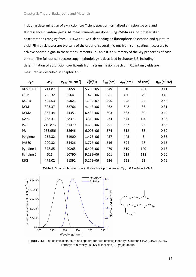
Chapter 2: Theory, Background and Materials
37
including determination of extinction coefficient spectra, normalised emission spectra and
fluorescence quantum yields. All measurements are done using PMMA as a host material at
concentrations ranging from 0.1 %wt to 1 wt% depending on fluorophore absorption and quantum
yield. Film thicknesses are typically of the order of several microns from spin coating, necessary to
achieve optimal signal in these measurements. In Table II is a summary of the key properties of each
emitter. The full optical spectroscopy methodology is described in chapter 3.3, including
determination of absorption coefficients from a transmission spectrum. Quantum yields are
measured as described in chapter 3.1.
Dye Mw εmax (M-1cm-1) Σ(ε(λ)) λabs (nm) λem (nm) Δλ (nm) ηQY (±0.02)
ADS067RE 711.87 5058 5.26E+05 349 610 261 0.11
C102 255.32 25641 1.42E+06 381 430 49 0.46
DCJTB 453.63 75021 1.13E+07 506 598 92 0.44
DCM 303.37 32766 4.14E+06 462 548 86 0.31
DCM2 355.44 44351 6.43E+06 503 583 80 0.44
DANS 268.31 28371 3.31E+06 434 574 140 0.33
PO 710.873 61479 4.63E+06 491 537 46 0.68
PR 963.956 58646 6.00E+06 574 612 38 0.60
Perylene 252.32 31900 1.47E+06 437 443 6 0.86
Ph660 290.32 34426 3.77E+06 516 594 78 0.15
Pyridine 1 378.85 40265 6.40E+06 479 619 140 0.13
Pyridine 2 526 60790 9.13E+06 501 619 118 0.20
R6G 479.02 91392 5.17E+06 536 558 22 0.76
Table II: Small molecular organic fluorophore properties at Cdye = 0.1 wt% in PMMA.
Figure 2.4.5: The chemical structure and spectra for blue emitting laser dye Coumarin 102 (C102); 2,3,6,7-
Tetrahydro-9-methyl-1H,5H-quinolizino(9,1-gh)coumarin.

Chapter 2: Theory, Background and Materials
38
Figure 2.4.6: The chemical structure and spectra for blue-green emitting perylene
Figure 2.4.7: The chemical structure and spectra for perylene red (PR), also known as Lumogen F Red 305.
Figure 2.4.8: The chemical structure and spectra for perylene orange (PO), also known as Lumogen F Orange
240.

Chapter 2: Theory, Background and Materials
39
Figure 2.4.9: The chemical structure and spectra for yellow-orange laser dye DCM; 4-(Dicyanomethylene)-2-
methyl-6-(4-dimethylaminostyryl)-4H-pyran
Figure 2.4.10: The chemical structure and spectra for red emitting laser dye DCM2; [2-methyl-6-[2-[(2,3,6,7-
tetrahydro-1H,5H-benzo[ij]quinolizin-9-yl)ethenyl]-4H-pyran-4-ylidene]propanedinitrile.
Figure 2.4.11: The chemical structure and spectra of red emitting laser dye DCJTB; 4-(Dicyanomethylene)-2-tert-
butyl-6-(1,1,7,7-tetramethyljulolidin-4-yl-vinyl)-4H-pyran.
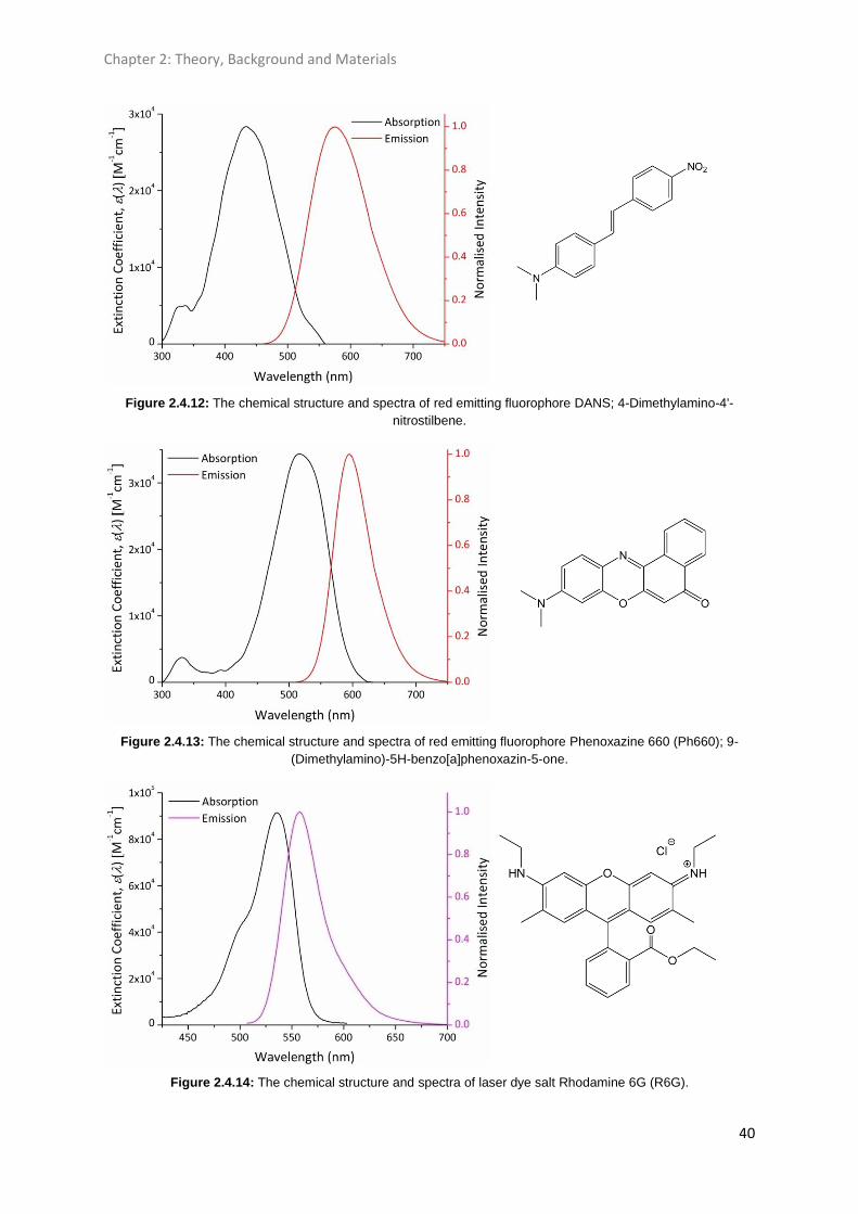
Chapter 2: Theory, Background and Materials
40
Figure 2.4.12: The chemical structure and spectra of red emitting fluorophore DANS; 4-Dimethylamino-4'-
nitrostilbene.
Figure 2.4.13: The chemical structure and spectra of red emitting fluorophore Phenoxazine 660 (Ph660); 9-
(Dimethylamino)-5H-benzo[a]phenoxazin-5-one.
Figure 2.4.14: The chemical structure and spectra of laser dye salt Rhodamine 6G (R6G).

Chapter 2: Theory, Background and Materials
41
Figure 2.4.15: The chemical structure and spectra of heavy metal complex ADS067RE; Iridium (III) bis(2-(2'-
benzo-thienyl)pyridinatoN,C3')(acetyl-acetonate).
Figure 2.4.16: The chemical structure and spectra of deep red emitting laser dye salt Pyridine 1; [2-[4-[4-
(dimethylamino)phenyl]-1,3-butadienyl]-1-ethylpyridinium monoperchlorate.
Figure 2.4.17: The chemical structure and spectra of deep red laser dye salt Pyridine 2; 4-[4-[4-
(dimethylamino)phenyl]-1,3-butadienyl]-1-ethyl-pyridinium perchlorate.
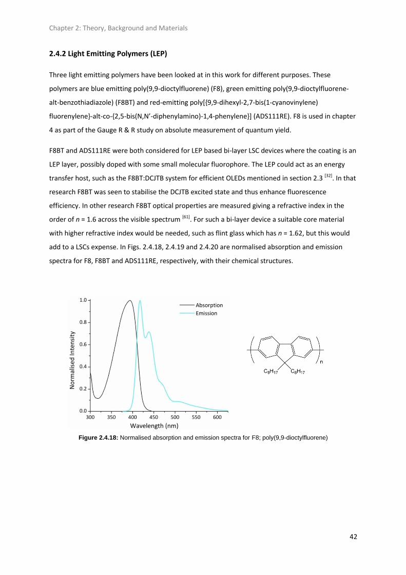
Chapter 2: Theory, Background and Materials
42
2.4.2 Light Emitting Polymers (LEP)
Three light emitting polymers have been looked at in this work for different purposes. These
polymers are blue emitting poly(9,9-dioctylfluorene) (F8), green emitting poly(9,9-dioctylfluorene-
alt-benzothiadiazole) (F8BT) and red-emitting poly[{9,9-dihexyl-2,7-bis(1-cyanovinylene)
fluorenylene}-alt-co-{2,5-bis(N,N’-diphenylamino)-1,4-phenylene}] (ADS111RE). F8 is used in chapter
4 as part of the Gauge R & R study on absolute measurement of quantum yield.
F8BT and ADS111RE were both considered for LEP based bi-layer LSC devices where the coating is an
LEP layer, possibly doped with some small molecular fluorophore. The LEP could act as an energy
transfer host, such as the F8BT:DCJTB system for efficient OLEDs mentioned in section 2.3 [32]. In that
research F8BT was seen to stabilise the DCJTB excited state and thus enhance fluorescence
efficiency. In other research F8BT optical properties are measured giving a refractive index in the
order of n = 1.6 across the visible spectrum [61]. For such a bi-layer device a suitable core material
with higher refractive index would be needed, such as flint glass which has n = 1.62, but this would
add to a LSCs expense. In Figs. 2.4.18, 2.4.19 and 2.4.20 are normalised absorption and emission
spectra for F8, F8BT and ADS111RE, respectively, with their chemical structures.
Figure 2.4.18: Normalised absorption and emission spectra for F8; poly(9,9-dioctylfluorene)

Chapter 2: Theory, Background and Materials
43
Figure 2.4.19: Normalised absorption and emission spectra for F8BT; poly(9,9-dioctylfluorene- alt-
benzothiadiazole)
Figure 2.4.20: Normalised absorption and emission spectra for ADS111RE; Poly[{9,9-dihexyl-2,7-bis(1-
cyanovinylene)fluorenylene}-alt-co-{2,5-bis(N,N’-diphenylamino)-1,4-phenylene}]
The spectral properties and quantum yield for these LEPs are summarised in Table III. As can be seen
quantum yields are too low for use in a LSC, although high stokes' shifts and small overlaps are
offered by F8BT and ADS111RE. F8x:F8BT1-x blends have been shown to achieve ηQY = 0.7 for x = 0.95
due to dipole-dipole coupling from F8 to F8BT [62]. Such methods using blends of LEPs could in
principle allow wide spectral coverage and efficient emission in the red.
Dye λabs (nm) λem (nm) Δλ (nm) ηQY (±0.02)
F8 394 417 23 0.45
F8BT 462 523 61 0.43
ADS111RE 408 648 240 0.11
Table III: Light emitting polymer properties.

Chapter 2: Theory, Background and Materials
44
2.4.3 Matrix/Host Materials
A number of polymeric host materials have been explored in this thesis though, as with literature,
the dominant host material has been poly(methyl methacrylate) (PMMA). This host has suitable and
well understood optical properties, and ease of processibility, making it an obvious choice for LSC
structures. Historically in LSC literature PMMA was the first host matrix material considered and to
date essentially all of the record LSC power conversion efficiencies have been made by devices using
this material.
As has been seen throughout sections 2.2 and 2.3 the properties of the host material must meet a
range of criteria to minimise losses and maximise the optical concentration. A high refractive index,
towards n2 = 2, is ideal to maximise the amount of light trapped inside the device after reflection loss
and ECL. Available polymer host materials exhibit indices in the range 1.3 < n2 < 1.6 so there is room
for improvement from polymer science. Polystyrene (PS) is the highest shown here with n = 1.596.
Specialist glasses can achieve higher refractive indices [35]; for example flint glass has 1.5 < n < 2.
Additionally glass is robust though it may add extra mass to a LSC device. Solar grade glass has
n = 1.47 according to one source [63] but with different fabrications methods will undoubtedly vary. It
is typically manufactured by either cast or float, costs in the region of £24 m-2 and £64 m-2,
depending on the fabrication route [64], and is a significant percentage of the cost of a PV panel.
However, this is of a similar order of cost to that of LSC structures fabricated with polymer host
materials, as is shown for PMMA in chapter 8.
The host material must provide a suitable environment for guest fluorophores. This must be inert, so
that the host does not act as a fluorescence quenching agent, and also offer low attenuation across
the visible spectrum. PMMA offers some of the best performance in this area with an absorption
coefficient of αh = 3.4x10⁻⁴ cm-1 at 550 nm [65]. This differs somewhat from polymer to polymer, for
example polycarbonate (PC) shows the greatest attenuation here at around 10-3 cm-1 at 550 nm [66].
A relatively new host material in LSC literature is poly(lactic acid) (PLA) which reportedly shows
similar attenuation to PMMA (measured by transmittance) and an oligothiophene fluorophore
exhibited greater quantum yield in PLA than PMMA [67]. PLA also offers a renewable, eco-friendly
alternative to petrochemical plastics.
A range of polymers for optical applications are summarised in Table IV with quantum yields
measured for the fluorophore DCM at Cdye = 0.1 wt%.
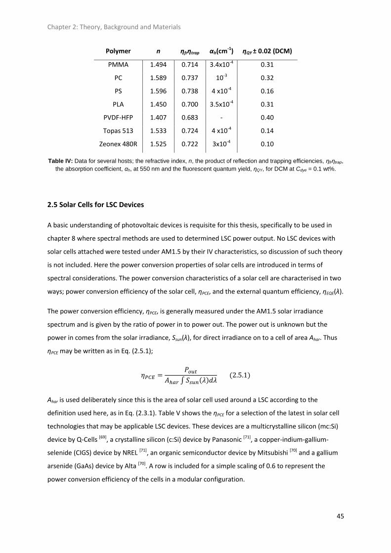
Chapter 2: Theory, Background and Materials
45
Polymer n ηfrηtrap αh(cm-1) ηQY ± 0.02 (DCM)
PMMA 1.494 0.714 3.4x10⁻⁴ 0.31
PC 1.589 0.737 10-3 0.32
PS 1.596 0.738 4 x10⁻⁴ 0.16
PLA 1.450 0.700 3.5x10⁻⁴ 0.31
PVDF-HFP 1.407 0.683 - 0.40
Topas 513 1.533 0.724 4 x10⁻⁴ 0.14
Zeonex 480R 1.525 0.722 3x10⁻⁴ 0.10
Table IV: Data for several hosts; the refractive index, n, the product of reflection and trapping efficiencies, ηfrηtrap,
the absorption coefficient, αh, at 550 nm and the fluorescent quantum yield, ηQY, for DCM at Cdye = 0.1 wt%.
2.5 Solar Cells for LSC Devices
A basic understanding of photovoltaic devices is requisite for this thesis, specifically to be used in
chapter 8 where spectral methods are used to determined LSC power output. No LSC devices with
solar cells attached were tested under AM1.5 by their IV characteristics, so discussion of such theory
is not included. Here the power conversion properties of solar cells are introduced in terms of
spectral considerations. The power conversion characteristics of a solar cell are characterised in two
ways; power conversion efficiency of the solar cell, ηPCE, and the external quantum efficiency, ηEQE(λ).
The power conversion efficiency, ηPCE, is generally measured under the AM1.5 solar irradiance
spectrum and is given by the ratio of power in to power out. The power out is unknown but the
power in comes from the solar irradiance, Ssun(λ), for direct irradiance on to a cell of area Ahar. Thus
ηPCE may be written as in Eq. (2.5.1);
Ahar is used deliberately since this is the area of solar cell used around a LSC according to the
definition used here, as in Eq. (2.3.1). Table V shows the ηPCE for a selection of the latest in solar cell
technologies that may be applicable LSC devices. These devices are a multicrystalline silicon (mc:Si)
device by Q-Cells [69], a crystalline silicon (c:Si) device by Panasonic [71], a copper-indium-gallium-
selenide (CIGS) device by NREL [71], an organic semiconductor device by Mitsubishi [70] and a gallium
arsenide (GaAs) device by Alta [70]. A row is included for a simple scaling of 0.6 to represent the
power conversion efficiency of the cells in a modular configuration.
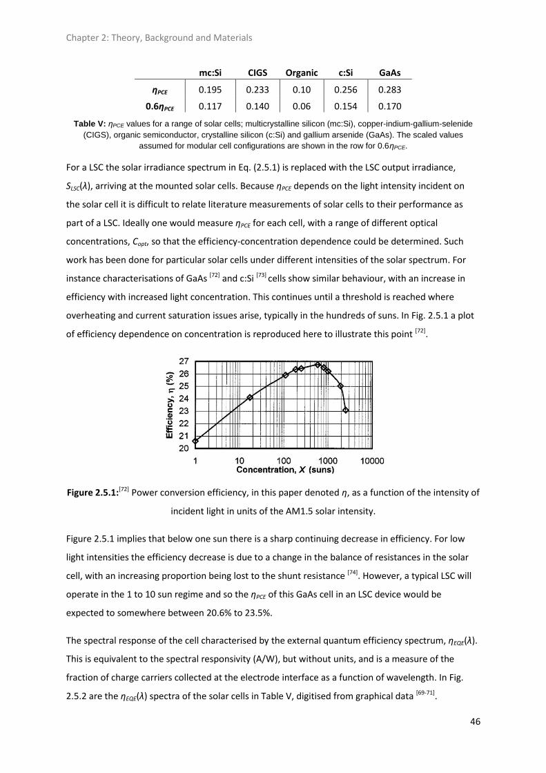
Chapter 2: Theory, Background and Materials
46
mc:Si CIGS Organic c:Si GaAs
ηPCE 0.195 0.233 0.10 0.256 0.283
0.6ηPCE 0.117 0.140 0.06 0.154 0.170
Table V: ηPCE values for a range of solar cells; multicrystalline silicon (mc:Si), copper-indium-gallium-selenide
(CIGS), organic semiconductor, crystalline silicon (c:Si) and gallium arsenide (GaAs). The scaled values
assumed for modular cell configurations are shown in the row for 0.6ηPCE.
For a LSC the solar irradiance spectrum in Eq. (2.5.1) is replaced with the LSC output irradiance,
SLSC(λ), arriving at the mounted solar cells. Because ηPCE depends on the light intensity incident on
the solar cell it is difficult to relate literature measurements of solar cells to their performance as
part of a LSC. Ideally one would measure ηPCE for each cell, with a range of different optical
concentrations, Copt, so that the efficiency-concentration dependence could be determined. Such
work has been done for particular solar cells under different intensities of the solar spectrum. For
instance characterisations of GaAs [72] and c:Si [73] cells show similar behaviour, with an increase in
efficiency with increased light concentration. This continues until a threshold is reached where
overheating and current saturation issues arise, typically in the hundreds of suns. In Fig. 2.5.1 a plot
of efficiency dependence on concentration is reproduced here to illustrate this point [72].
Figure 2.5.1:[72] Power conversion efficiency, in this paper denoted η, as a function of the intensity of
incident light in units of the AM1.5 solar intensity.
Figure 2.5.1 implies that below one sun there is a sharp continuing decrease in efficiency. For low
light intensities the efficiency decrease is due to a change in the balance of resistances in the solar
cell, with an increasing proportion being lost to the shunt resistance [74]. However, a typical LSC will
operate in the 1 to 10 sun regime and so the ηPCE of this GaAs cell in an LSC device would be
expected to somewhere between 20.6% to 23.5%.
The spectral response of the cell characterised by the external quantum efficiency spectrum, ηEQE(λ).
This is equivalent to the spectral responsivity (A/W), but without units, and is a measure of the
fraction of charge carriers collected at the electrode interface as a function of wavelength. In Fig.
2.5.2 are the ηEQE(λ) spectra of the solar cells in Table V, digitised from graphical data [69-71].
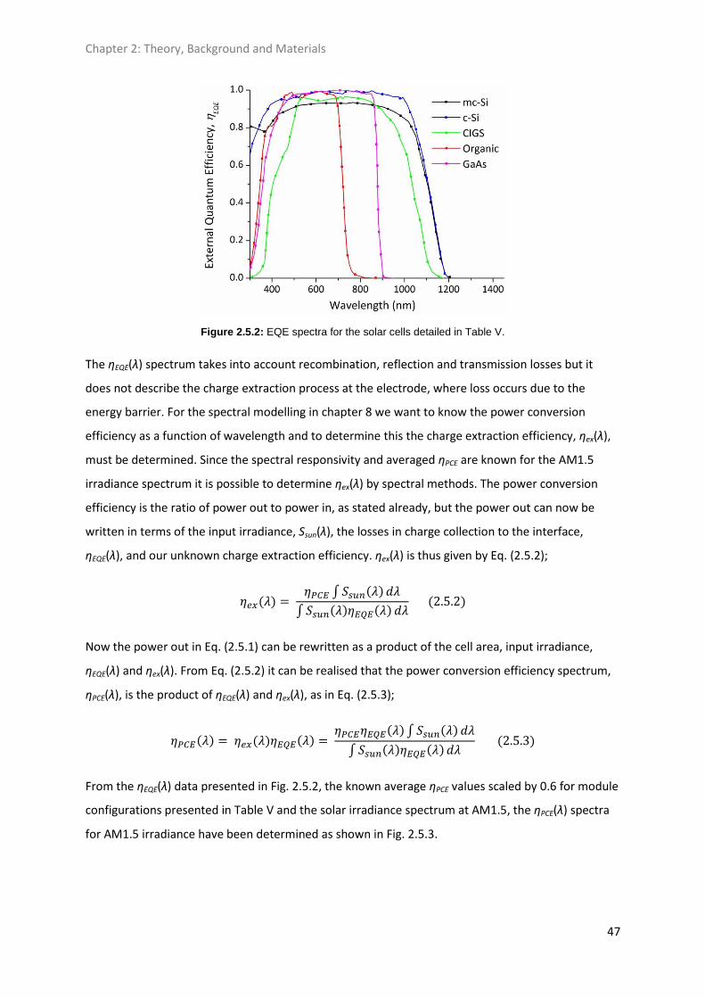
Chapter 2: Theory, Background and Materials
47
Figure 2.5.2: EQE spectra for the solar cells detailed in Table V.
The ηEQE(λ) spectrum takes into account recombination, reflection and transmission losses but it
does not describe the charge extraction process at the electrode, where loss occurs due to the
energy barrier. For the spectral modelling in chapter 8 we want to know the power conversion
efficiency as a function of wavelength and to determine this the charge extraction efficiency, ηex(λ),
must be determined. Since the spectral responsivity and averaged ηPCE are known for the AM1.5
irradiance spectrum it is possible to determine ηex(λ) by spectral methods. The power conversion
efficiency is the ratio of power out to power in, as stated already, but the power out can now be
written in terms of the input irradiance, Ssun(λ), the losses in charge collection to the interface,
ηEQE(λ), and our unknown charge extraction efficiency. ηex(λ) is thus given by Eq. (2.5.2);
Now the power out in Eq. (2.5.1) can be rewritten as a product of the cell area, input irradiance,
ηEQE(λ) and ηex(λ). From Eq. (2.5.2) it can be realised that the power conversion efficiency spectrum,
ηPCE(λ), is the product of ηEQE(λ) and ηex(λ), as in Eq. (2.5.3);
From the ηEQE(λ) data presented in Fig. 2.5.2, the known average ηPCE values scaled by 0.6 for module
configurations presented in Table V and the solar irradiance spectrum at AM1.5, the ηPCE(λ) spectra
for AM1.5 irradiance have been determined as shown in Fig. 2.5.3.

Chapter 2: Theory, Background and Materials
48
Figure 2.5.3: PCE spectra for the solar cells detailed in Table V calculated using the scaled average ηPCE with
Eq. (2.5.3).
Note that separating the ηPCE into a wavelength dependent function is of an unphysical basis because
it is given by the maximum power point on a solar cell's IV curve. It works because the spectral
methods defined here are essentially a normalisation relative to the AM1.5 irradiance spectrum. The
integral of the product of power conversion spectra in 2.5.3 and the AM1.5 irradiance spectrum, as a
ratio of the integral of the input irradiance, gives the scaled ηPCE values in Table V, as required by
definition.
The power generated by a solar cell, Pout, can now be written as the product of the PV area, Ahar, and
the integral of the product of ηPCE(λ) and Ssun(λ), as in Eq. (2.5.4);
It must be highlighted that the light intensity falling on the cell will vary between different LSC
designs and any model must be able to take account of this fact in light of Fig. 2.5.1. Because such in
depth data is not available for the solar cells studied here an estimation of efficiency versus
concentration for the cells is built from literature [72,73,75]. In particular J. F. Randall and J. Jacot
(2002)[75] show that the form of the dependence is roughly the same for eight different solar cells,
but the peak efficiency varies with respect to concentration. Choosing an optical concentration, Copt,
range between 0.01 and 100 suns using the data for GaAs[72,75] and c:Si[73,75] we get a straight curve in
log space, similar to Fig. 2.5.1. From this a power correction factor, β, can be defined as the ratio of
ηPCE as a function of Copt to the ηPCE under one sun at AM1.5, thus β is equal to unity when Copt = 1
sun, as shown in Fig. 2.5.4. Then Eq. (2.5.4) becomes;
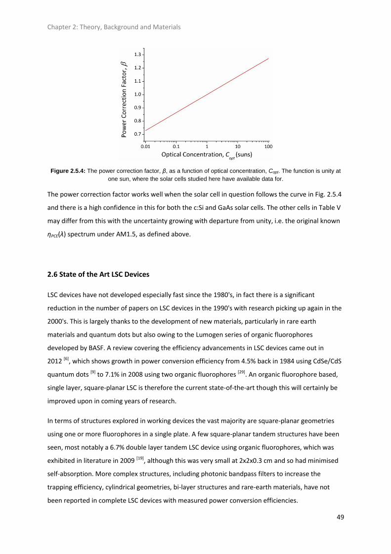
Chapter 2: Theory, Background and Materials
49
Figure 2.5.4: The power correction factor, β, as a function of optical concentration, Copt. The function is unity at
one sun, where the solar cells studied here have available data for.
The power correction factor works well when the solar cell in question follows the curve in Fig. 2.5.4
and there is a high confidence in this for both the c:Si and GaAs solar cells. The other cells in Table V
may differ from this with the uncertainty growing with departure from unity, i.e. the original known
ηPCE(λ) spectrum under AM1.5, as defined above.
2.6 State of the Art LSC Devices
LSC devices have not developed especially fast since the 1980's, in fact there is a significant
reduction in the number of papers on LSC devices in the 1990's with research picking up again in the
2000's. This is largely thanks to the development of new materials, particularly in rare earth
materials and quantum dots but also owing to the Lumogen series of organic fluorophores
developed by BASF. A review covering the efficiency advancements in LSC devices came out in
2012 [6], which shows growth in power conversion efficiency from 4.5% back in 1984 using CdSe/CdS
quantum dots [9] to 7.1% in 2008 using two organic fluorophores [29]. An organic fluorophore based,
single layer, square-planar LSC is therefore the current state-of-the-art though this will certainly be
improved upon in coming years of research.
In terms of structures explored in working devices the vast majority are square-planar geometries
using one or more fluorophores in a single plate. A few square-planar tandem structures have been
seen, most notably a 6.7% double layer tandem LSC device using organic fluorophores, which was
exhibited in literature in 2009 [19], although this was very small at 2x2x0.3 cm and so had minimised
self-absorption. More complex structures, including photonic bandpass filters to increase the
trapping efficiency, cylindrical geometries, bi-layer structures and rare-earth materials, have not
been reported in complete LSC devices with measured power conversion efficiencies.

Chapter 2: Theory, Background and Materials
50
A pick of some of the best LSC devices through their short history, with their configurations and
components, is exhibited in Table VI. As can be seen in Table VI the best devices from the 1980's
were of a larger size compared to those of the 2000's, for which the latter must owe some of their
improved efficiency for. Furthermore the two best devices use III-V semiconductor solar cells which,
based on the analysis in section 2.5, undoubtedly improve efficiency over c:Si cells. The modern
devices really therefore stand as interesting demonstrations, but not as significant advancements. As
the authors of M. Debije et. al. (2012)[6] state; the key issues to overcome are still inefficiencies in
the fluorophore and the lack of intense collaborative effort between the disparate groups working
on the technology across the world. This is in contrast to the many photovoltaic technologies which
have received far greater attention and concerted effort.
Fluorophore L x L x W (cm) G Solar Cell (# sides) ηLSC (%) Year Reference
DCM 120 x 100 x 0.4 68.18 c:Si (4) 1.3 1981 [40]
Coumarin, Rhodamine 140 x 140 x 3 11.67 c:Si (4) 3.2 1984 [12]
CdSe/CdS QDs 140 x 140 x 3 11.67 GaAs (4) 4.5 1984 [12]
CRS040, PR 5 x 5 x 0.5 2.5 GaAs (4) 7.1 2008 [29]
BA241,BA856 2 LSCs at 2 x 2 x 0.3 1.67 GaInP (4) 6.7 2009 [25]
Perylene perinone, PR 2 LSCs at 5 x 5 x 0.5 2.5 c:Si (2) 4.2 2012 [76]
Table VI: A pick of the best LSC devices through the technology's history is shown here. The last two entries are
two layer tandem LSC devices and the last entry has two mirrored edges and two edges with c:Si cells
connected.
Calculations to determine the cost of LSC devices to explore the economic value of the technology
can be found in several places with different approaches [30, 76]. In the most recent work Bende et. al.
(2008) use a ray-tracing model to optimise the relative cost and relative power density between LSC
and standard PV devices. Optimisation is also performed on fluorophore concentration of the
organic dye, Yellow CRS040 but PR is used extensively in the models. For cost calculations the model
uses the polymer plate cost per unit area as a ratio to the conventional PV cost per unit area as a key
parameter. They show that when this quantity is 1/15 the LSC would cost 35% and would generate
21% of the power of conventional PV. By the time this ratio is 1/5 the LSC costs as much as the
conventional PV but only generates 22% of the power, at which point you would just use
conventional PV.
Chapter 2: Theory, Background and Materials
51
2.8 References
[1] G. Smestad, H. Ries, R. Winston and E. Yablonovitch, The Thermodynamic Limits of Light
Concentrators, Solar Energy Mater. 21, 99 – 111 (1990)
[2] R. Winston, J. C. Minano and P. Benitez, Non-imaging Optics, Elsevier Academic Press, Chap. 1, 2 -
6 (2005)
[3] A. Goetzberger and V. Wittwer, Fluorescent Planar Collector-Concentrators: A Review, Solar Cells
4, 3 – 23 (1981)
[4] J. S. Batchelder, A. H. Zewail, and T. Cole, Luminescent Solar Concentrators 1: Theory of
Operation and Techniques for Performance Evaluation, Applied Optics 18, 18, 3090 - 3110 (1979)
[5] P. P. C. Verbunt, C. Sánchez-Somolinos, D. J. Broer and M. G. Debije, Anisotropic light emissions in
luminescent solar concentrators-isotropic systems, Opt. Express 21, S3, A485-A493 (2013)
[6] M. G. Debije and P. P. C. Verbunt, Thirty Years of Luminescent Solar Concentrator Research: Solar
Energy for the Built Environment, Adv. Energy Mater. 2, 12 – 35 (2012)
[7] A. A. Earp, G. B. Smith, P. D. Swift and J. Franklin, Maximising the Light Output of a Luminescent
Solar Concentrator, Solar Energy 76, 655 667 (2004)
[8] R. Reisfeld, New Developments in Luminescence for Solar Energy Utilization, Opt. Mater. 32 850-
856 (2010)
[9] Freidman, P. S. and Parent, C. R. Luminescent Solar Concentrator Development - Final
Subcontract Report, Solar Energy Research Institute, U.S. DOE contract No. DE-AC02-83CH10093
(1987)
[10] M. A. El-Shahawy and A. F. Mansour, Optical Properties of Some Luminescent Solar
Concentrators, J. Mater. Sci. Mater. Elec., 7, 171 – 174 (1996)
[11] J. Mugnier, Y. Dordet, J. Pouget and B. Valeur, A Photometric Approach of Fluorescent Solar
Concentrators. Role of Diffuse Reflectors and Spectral Sensitivity of Solar Cells, Revue Phys. Appl. 22,
89-100 (1987)
[12] L. R. Wilson, Thesis on Luminescent Solar Concentrators: A Study of Optical Properties, Re-
absorption and Device Optimisation, Bryce Richards’ group in Edinburgh (2010)

Chapter 2: Theory, Background and Materials
52
[13] M. N. Polyanskiy, RefractiveIndex.INFO (2013)
http://refractiveindex.info/legacy/?wavelength=0.55
[14] R. Sóti, É. Farkas, M. Hilbert, Zs. Farkas, I. Ketskeméty, Photon transport in luminescent solar
concentrators, J. Lumin. 68, 105 - 114 (1996)
[15] K. R. McIntosh, N. Yamada and B. S. Richards, Theoretical Comparison of Cylindrical and Square-
Planar Luminescent Solar Concentrators, App. Phys. B 88, 285-290 (2007)
[16] O. Y. Edelenbosch, M. Fisher, L. Patrignani, W. G. J. H. M. van Sark and A. J. Chatten,
Luminescent Solar Concentrators with Fiber Geometry, Optics Express 21, S3, 503 - 514 (2013)
[17] R. Bose, D. J. Farrell, A. J. Chatten, M. Pravettoni, A. Büchtemann and K. W. J. Barnham, Novel
Configurations of Luminescent Solar Concentrators, Proc. 22nd European Photovoltaic Solar Energy
Conference, pp. 210-214, (2007)
[18] Uwe Rau, Florian Einsele and Gerda C. Glaeser, Efficiency Limits of Photovoltaic Fluorescent
Concentrators, Appl. Phys. Lett. 87, 171101 (2005)
[19] J. C. Goldschmidt, M. Peters, A. Bösch, H. Helmers, F. Dimroth, S. W. Glunz and G. Willeke,
Increasing the Efficiency of Fluorescent Concentrator Systems, Sol. En. Mater. Sol. Cells 93, 176 - 182
(2009)
[20] M. G. Debije, R. H. L. van Der Blom, D. J. Broer and C. W. M. Bastiaansen, Using selectively
reflecting organic mirrors to improve light output from a luminescent solar concentrator, in Proc.
World Renewable Energy Congress IX (2006)
[21] M. G. Debije, M. P. Van, P. P. Verbunt, M. J. Kastelijn, R. H. L. van Der Blom, D. J. Broer and C. W.
M. Bastiaansen, Effect on the output of a luminescent solar concentrator on application of organic
wavelength-selective mirrors, Appl. Opt. 49, 4, 745-751 (2010)
[22] B. C. Rowan, L. R. Wilson and B. S. Richards, Advanced Material Concepts for Luminescent Solar
Concentrators, IEEE Journal of Selected Topics in Quantum Electronics. 14, 5 (2008)
[23] B. A. Swartz, T. Cole and A. H. Zewail, Photon Trapping and Energy Transfer in Multiple-Dye
Plastic Matrices: an Efficient Solar-Energy Concentrator, Opt. Lett. 1, 2, 73 - 75 (1977)
[24] S. Chandra, J. Doran, S. McCormack, M. Kennedy and A. Chatten, Enhanced Quantum Dot
Emission for Luminescent Solar Concentrators using Plasmonic Interaction, Sol. Energy Mater. & Sol.
Cells 98, 385 - 390 (2012)
Chapter 2: Theory, Background and Materials
53
[25] S. Tsoi, Dirk J. Boer, C. W. M. Bastiaansen and M. G. Debije, Using Lenses to Improve the Output
of a Patterned Luminescent Solar Concentrator, Adv. Energy Mater. (2012),
doi: 10.1002/aenm.201200395
[26] C. L. Mulder, P. D. Reusswig, A. M. Velázquez, H. Kim, C. Rotschild and M. A. Baldo, Dye
Alignment in Luminescent Solar Concentrators: I. Vertical Alignment for Improved Waveguide
Coupling, Optics Express 18, S1 (2010)
[27] Y. Zhang, K. Aslan, M. Previte and C. Geddes, Metal-enhanced Fluorescence: Surface Plasmons
Can Radiate a Fluorophore's Structured Emission, App. Phys. Lett. 90, 053107 (2007)
[28] S. Wang, D.-A. Borca-Tasciuc and D. Kaminski, Spectral Coupling of Fluorescence Solar
Concentrators to Plasmonic Solar Cells, J. App. Phys. 109, 7, 074910 (2011)
[29] L. H. Slooff, E. E. Bende, A. R. Burgers, T. Budel, M. Pravettoni, R. P. Kenny, E. D. Dunlop and A.
Büchtemann, A Luminescent Solar Concentrator with 7.1% Power Conversion Efficiency, Phys. Stat.
Sol. (RRL) 2, 257-259 (2008)
[30] M. J. Currie, J. K. Mapel, T. D. Heidel, S. Goffri and M. A. Baldo, High Efficiency Organic Solar
Concentrators for Photovoltaics, Science 321, 226 - 228 (2008)
[31] S. T. Bailey, G. E. Lokey, M. S. Hanes, J. D. M. Shearer, J. B. McLafferty, G. T. Beaumont, T. T.
Baseler, J. M. Layhue, D. R. Broussard, Y. Zhang, J. B. Wittmershaus, Optimised excitation energy
transfer in a three-dye luminescent solar concentrator, Sol. En. Mater. Sol. Cells 91, 67 -75 (2007)
[32] P. Chiu, C. Huang, C. Yang, T. Meen and Y. Wang, Red polymer light-emitting devices based on
dye-dispersed poly(9,9-dioctylfluorene-alt-benzothiadiazole), Micro. Relia. 50, 5, 692-695 (2010)
[33] Y. Hasegawa, Y. Wada and S. Yanagida, Strategies for the design of luminescent lanthanide (III)
complexes and their photonic applications, J. Photochem. Photobiol. C: Photochem. Rev. 5, 3, 183-
202 (2004)
[34] J. Gordon, J. Ballato, J. Jin and D. W. Smith Jr., Spectroscopic Properties as a Function of Fluorine
Content in Eu3+:PMMA, J. Polym. Sci. B: Polym. Phys. 44, 11, 1592 - 1596 (2006)
[35] S. J. Gallagher, P. C. Eames and B. Norton, Quantum dot solar concentrator behaviour, predicted
using a ray tracing approach, Int. J. Ambient Energy, 25, 47 (2004)
[36] P. Prentice, Influence of molecular weight on the fracture of poly(methyl methacrylate)
(PMMA), Polymer 24, 3, 344 - 350 (1983)
Chapter 2: Theory, Background and Materials
54
[37] R. Reisfeld, Fluorescent dyes in sol-gel glasses, J. Fluor. 12, 3, 317 - 325 (2002)
[38] J. C. Goldschmidt, M. Peters, L. Prönneke, L. Steidl, R. Zentel, B. Bläsi, A. Gombert, S. Glunz, G.
Willeke and U. Rau, Theoretical and Experimental Analysis of Photonic Structures for Fluorescent
Concentrators with Increased Efficiencies, Phys. Stat. Sol. (a) 205, 12, 2811 - 2821 (2008)
[39] H. Hernandez-Noyola, D. H. Potterveld, R. J. Holt and S. B. Darling, Optimising Luminescent Solar
Concentrator Design, Energy Environ. Sci. 5, 5798 – 5802 (2012)
[40] J. S. Batchelder, A. H. Zewail, and T. Cole, Luminescent Solar Concentrators 2: Experimental and
Theoretical Analysis of their Possible Efficiencies, Applied Optics 20, 21, 3733 - 3754 (1981)
[41] L. H. Sloof, T. Budel, A. R. Burgers, N. J. Bakker, R. Danz, T. Meyer and A. Meyer, The
Luminescent Concentrator: Stability Issues, in Proc. 22nd European Photovoltaic Solar Energy
Conference (2007)
[42] L. R. Wilson and B. S. Richards, High-efficiency Dyes for Luminescent Solar Concentrators, in
Proc. 23rd European Photovoltaic Solar Energy Conference (2008)
[43] K. W. J. Barnham, J. L. Marques, J. Hassard and P. OBrien, Quantum-dot Concentrator and
Thermodynamic Model for the Global Redshift, Appl. Phys. Lett. 76, 9, 1197 (2000)
[44] G. V. Shcherbatyuk, R. H. Inman, C. Wang, R. Winston and S. Ghosh, Viability of Using Near
Infrared PbS Quantum Dots as Active Materials in Luminescent Solar Concentrators, Appl. Phys. Lett.
96, 19, 191901 (2010)
[45] D. V. Talapin, J. H. Nelson, E. V. Shevchenko, S. Aloni, B. Sadtler and A. P. Alivisatos, Seeded
Growth of Highly Luminescent CdSe/CdS Nanoheterostructures with Rod and Tetrapod
Morphologies, Nano Letters 7, 10, 2951-2959 (2007)
[46] B. C. Rowan, L. R. Wilson and B. S. Richards, Visible and Near-infrared Emitting Lanthanide
Complexes for Luminescent Solar Concentrators, in Proc. 24th European Photovoltaic Solar Energy
Conference (2009)
[47] L. R. Wilson, B. C. Rowan, N. Robertson, O. Moudam, A. C. Jones and B. S. Richards,
Characterisation and Reduction of Reabsorption Losses in Luminescent Solar Concentrators, Applied
Optics 49, 1651 (2010)
[48] R. Reisfeld, Industrial Applications of Rare Earths in Fiber Optics, Luminescent Solar
Concentrators and Lasers, Inorganica Chimica Acta 95, 69-74 (1984)
Chapter 2: Theory, Background and Materials
55
[49] http://www.life.illinois.edu/govindjee/biochem494/Abs.html
[50] A. D. Stein and M. D. Fayer, Nanosecond timescale optical inhomogeneous broadening of dye
molecules in liquids at and near room temperature, Chem. Phys. Lett. 176, 2, 159 - 166 (1991)
[51] Y. Kawamura, J. Brooks, J. J. Brown, H. Sasabe and C. Adachi, Intermolecular Interaction and a
Concentration-Quenching Mechanism of Phosphorescent Ir(III) Complexes in a Solid Film, Phys. Rev.
Lett. 96, 017404 (2006)
[52] Rabih O. Al-Kaysi et. al., The Photophysical Properties of Chromophores at High (100mM and
above) Concentrations in Polymers and as Neat Solids, Phys. Chem. Chem. Phys. 8, 3453-3459, (2006)
[53] S. A. Bagnich and V. N. Knyukshto, Quenching of Fluorescence of Conjugated Poly(p-Pheylene)
Polymers by Benzil and Dimethylaminobenzil Molecules, J. Appl. Spec. 73, 6 (2006)
[54] P. L. Burn, S. Lo and I. D. W. Samuel, The Development of Light Emitting Dendrimers for
Displays, Adv. Mater. 19, 1675 - 1688 (2007)
[55] M. Shimizu and T. Hiyama, Organic Fluorophores Exhibiting Highly Efficient Photoluminescence
in the Solid State, Chem. Asian J. 5, 1516 - 1531 (2010)
[56] J. R. Lakowicz, Principles of Fluorescence Spectroscopy, 3rd ed. (Springer, Singapore, 2006),
Chap. 6, pp. 205–213.
[57] C. F. Madigan and V. Bulović, Solid State Solvation in Amorphous Organic Thin Films, Phys. Rev.
Lett. 91, 247403 (2003)
[58] V. Bulović, R. Deshpande, M. E. Thompson and S. R. Forrest, Tuning the Colour Emission of Thin
Film Molecular OLEDs by the Solid State Solvation Effect, Chem. Phys. Lett. 308, 317 - 322 (1999)
[59] A. K. Sheridan, A. R. Buckley, a. M. Fox, A. Bacher, D. D. C. Bradley and I. D. W. Samuel, Efficient
energy transfer in organic thin films - implications for organic lasers, J. Appl. Phys. 92, 6367 (2003)
[60] W. G. J. H. M. van Sark et. al., Luminescent Solar Concentrators - A Review of Recent Results,
Opt. Exp. 16, 26, 21773 (2008)
[61] C. M. Ramsdale and N. C. Greenham, The optical constants of emitter and electrode materials in
polymer light-emitting diodes, J. Phys. D: Appl. Phys. 36, L29 - L34 (2003)
[62] A. J. Cadby and D. G. Lidzey et. al., Imaging the Fluorescence Decay Lifetime of a Conjugated
Polymer Blend By Using a Scanning Near-Field Optical Microscope, Adv. Mater. 19, 107 - 111 (2007)
Chapter 2: Theory, Background and Materials
56
[63] M. Junghänel, M. Schädel, L. Stolze and S. Peters, Black Multicrystalline Solar Modules Using
Novel Multilayer Antireflection Stacks, Proc. 25th European Photovoltaic Solar Energy Conference,
pp. 2637-2641 (2010)
[64] Solar Glass & Mirrors, Green Rhino Energy (2013)
http://www.greenrhinoenergy.com/solar/technologies/solar_glass.php
[65] G. Colantuono, A. Buckley and R. Erdélyi, Ray-Optics Modelling of Rectangular and Cylindrical 2-
Layer Solar Concentrators, J. Light. Tech. 31, 7, 1033-1044 (2013)
[66] Paradigm Optics Inc., 2000-2012, http://www.paradigmoptics.com/pof/poffaqs.html
[67] V. Fattori, M. Melucci, L. Ferrante, M. Zambianchi, I. Manet, W. Oberhauser, G. Giambastiani, M.
Frediani, G. Giachi and N. Camaioni, Poly(lactic acid) as a transparent matrix for luminescent solar
concentrators: a renewable material for a renewable energy technology, Energy Environ. Sci. 4, 2849
- 2853 (2011)
[68] Best Research PCE Values, NREL (2013), http://www.nrel.gov/ncpv/
[69] M. A. Green, K. Emery, Y. Hishikawa, W. Warta and E. D. Dunlop, Solar Cell Efficiency Tables
(Version 38), Prog. Photovolt: Res. Appl. 19, 565-572 (2011)
[70] M. A. Green, K. Emery, Y. Hishikawa, W. Warta and E. D. Dunlop, Solar Cell Efficiency Tables
(Version 39), Prog. Photovolt: Res. Appl. 20, 12-20 (2012)
[71] M. A. Green, K. Emery, Y. Hishikawa, W. Warta and E. D. Dunlop, Solar Cell Efficiency Tables
(Version 44), Prog. Photovolt: Res. Appl. 22, 701-710 (2014)
[72] C. Algora, E. Ortiz, I. Rey-Stolle, V. Díaz, R. Peña, V. M. Andreev, V. P. Khvostikov and V. D.
Rumyantsev, A GaAs Solar Cell with an Efficiency of 26.2% at 1000Suns and 25% at 2000 Suns, IEEE
Transactions on Electron Devices 48, 5, 840-844 (2001)
[73] R. McConnell and V. Fthenakis, Third Generation Photovoltaics (Intech, 2012), Chap. 7, pp. 167-
168
[74] G. Bunea, K. Wilson, Y. Meydbray, M. Campbell and D. D. Ceuster, Low Light Performance of
Mono-Crystalline Silicon Solar Cells, in Proc. 4th World Conference on Photovoltaic Energy
Conversion, pp. 1312-1314 (2006)
[75] J. F. Randall and J. Jacot, The Performance and Modelling of 8 Photovoltaic Materials Under
Variable Light Intensity and Spectra, in Proc. World Renewable Energy Congress (2002)

Chapter 2: Theory, Background and Materials
57
[75] L. Desmet, A. J. M. Ras, D. K. G. de Boer and M. G. Debije, Monocrystalline silicon photovoltaic
luminescent solar concentrator with 4.2% power conversion efficiency, Opt. Lett. 37, 15, 3087 - 3089
(2012)
[76] E. E. Bende, L. H. Slooff, A. R. Burgers, W. G. J. H. M. van Sark and M. Kennedy, Cost & Efficiency
Optimisation of the Fluorescent Solar Concentrator, in Proc. 23rd European Photovoltaic Solar
Energy Conference (2008)
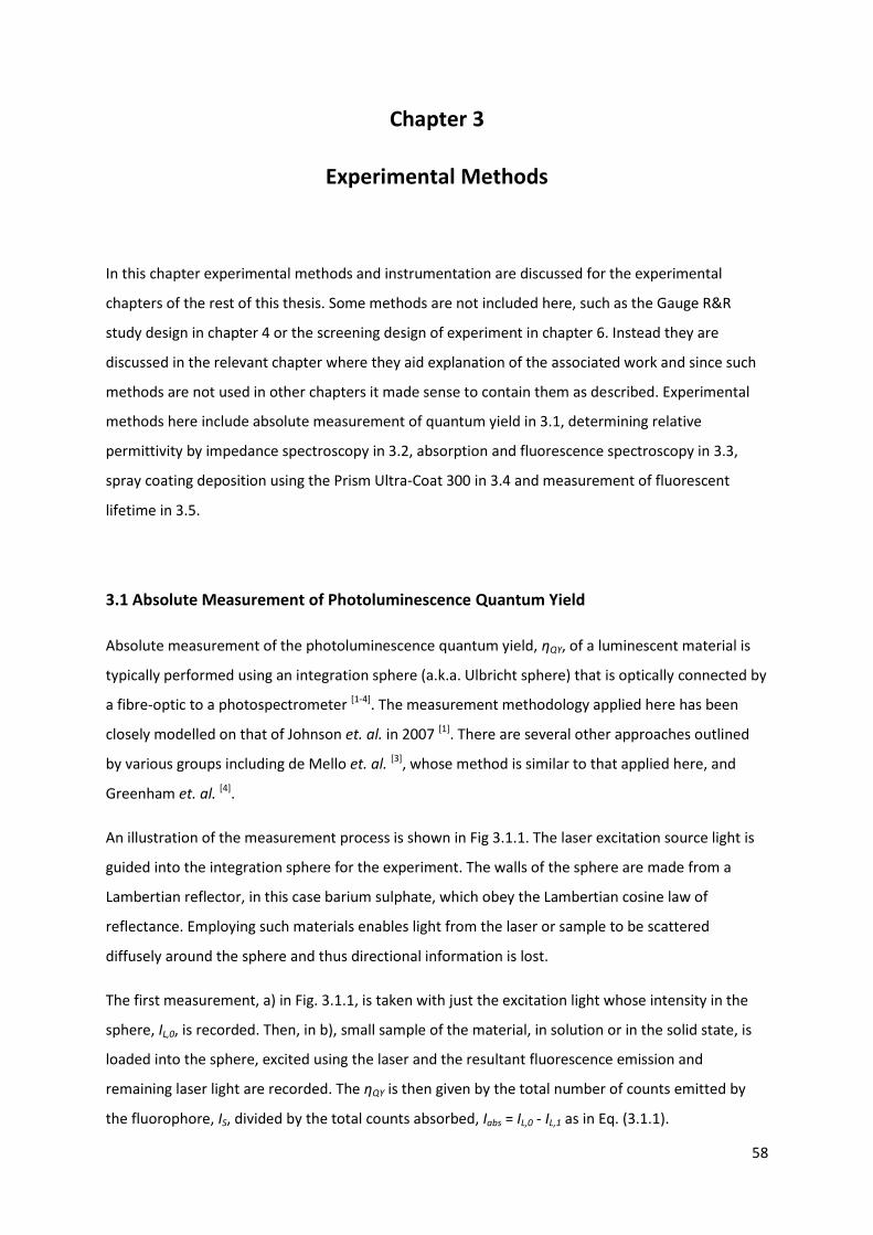
58
Chapter 3
Experimental Methods
In this chapter experimental methods and instrumentation are discussed for the experimental
chapters of the rest of this thesis. Some methods are not included here, such as the Gauge R&R
study design in chapter 4 or the screening design of experiment in chapter 6. Instead they are
discussed in the relevant chapter where they aid explanation of the associated work and since such
methods are not used in other chapters it made sense to contain them as described. Experimental
methods here include absolute measurement of quantum yield in 3.1, determining relative
permittivity by impedance spectroscopy in 3.2, absorption and fluorescence spectroscopy in 3.3,
spray coating deposition using the Prism Ultra-Coat 300 in 3.4 and measurement of fluorescent
lifetime in 3.5.
3.1 Absolute Measurement of Photoluminescence Quantum Yield
Absolute measurement of the photoluminescence quantum yield, ηQY, of a luminescent material is
typically performed using an integration sphere (a.k.a. Ulbricht sphere) that is optically connected by
a fibre-optic to a photospectrometer [1-4]. The measurement methodology applied here has been
closely modelled on that of Johnson et. al. in 2007 [1]. There are several other approaches outlined
by various groups including de Mello et. al. [3], whose method is similar to that applied here, and
Greenham et. al. [4].
An illustration of the measurement process is shown in Fig 3.1.1. The laser excitation source light is
guided into the integration sphere for the experiment. The walls of the sphere are made from a
Lambertian reflector, in this case barium sulphate, which obey the Lambertian cosine law of
reflectance. Employing such materials enables light from the laser or sample to be scattered
diffusely around the sphere and thus directional information is lost.
The first measurement, a) in Fig. 3.1.1, is taken with just the excitation light whose intensity in the
sphere, IL,0, is recorded. Then, in b), small sample of the material, in solution or in the solid state, is
loaded into the sphere, excited using the laser and the resultant fluorescence emission and
remaining laser light are recorded. The ηQY is then given by the total number of counts emitted by
the fluorophore, IS, divided by the total counts absorbed, Iabs = IL,0 - IL,1 as in Eq. (3.1.1).
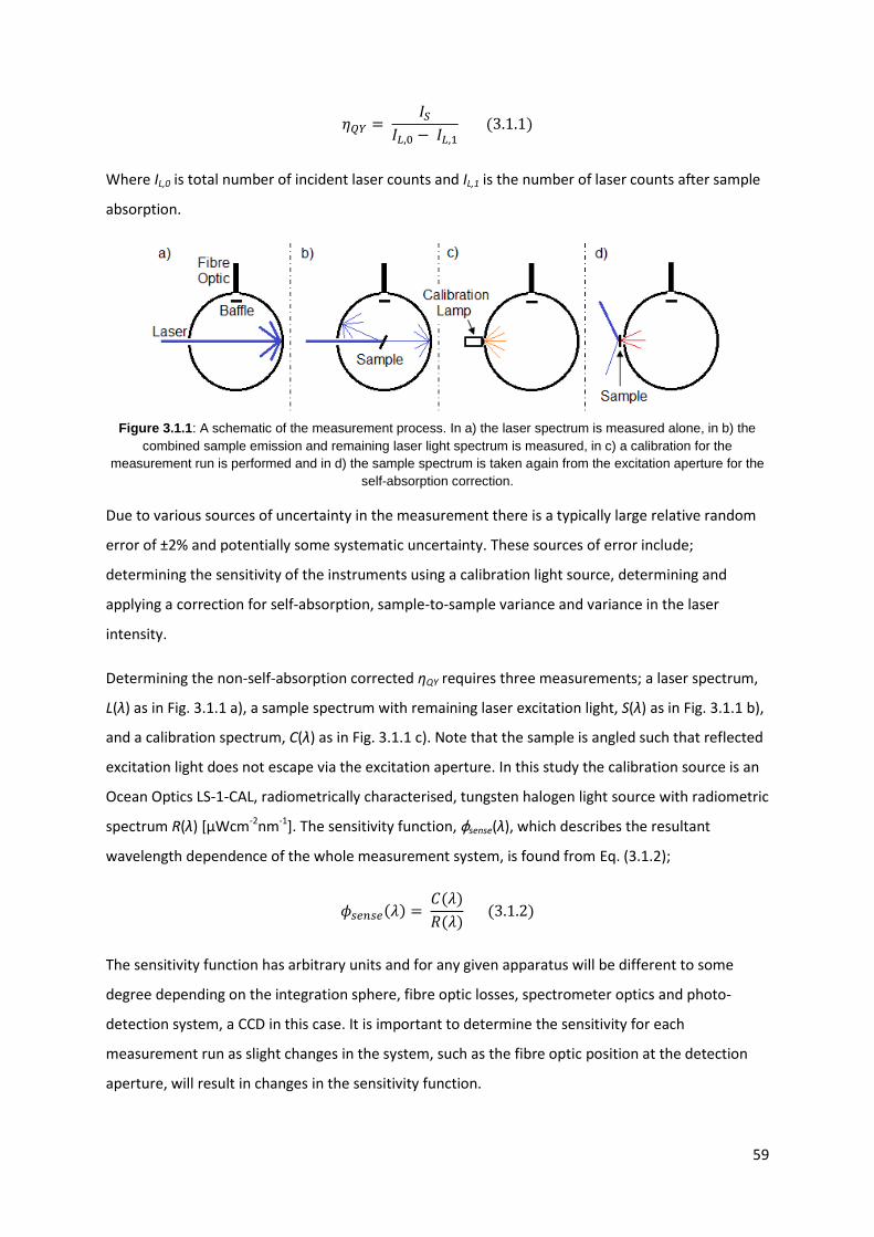
59
Where IL,0 is total number of incident laser counts and IL,1 is the number of laser counts after sample
absorption.
Figure 3.1.1: A schematic of the measurement process. In a) the laser spectrum is measured alone, in b) the
combined sample emission and remaining laser light spectrum is measured, in c) a calibration for the
measurement run is performed and in d) the sample spectrum is taken again from the excitation aperture for the
self-absorption correction.
Due to various sources of uncertainty in the measurement there is a typically large relative random
error of ±2% and potentially some systematic uncertainty. These sources of error include;
determining the sensitivity of the instruments using a calibration light source, determining and
applying a correction for self-absorption, sample-to-sample variance and variance in the laser
intensity.
Determining the non-self-absorption corrected ηQY requires three measurements; a laser spectrum,
L(λ) as in Fig. 3.1.1 a), a sample spectrum with remaining laser excitation light, S(λ) as in Fig. 3.1.1 b),
and a calibration spectrum, C(λ) as in Fig. 3.1.1 c). Note that the sample is angled such that reflected
excitation light does not escape via the excitation aperture. In this study the calibration source is an
Ocean Optics LS-1-CAL, radiometrically characterised, tungsten halogen light source with radiometric
spectrum R(λ) [µWcm-2nm-1]. The sensitivity function, φsense(λ), which describes the resultant
wavelength dependence of the whole measurement system, is found from Eq. (3.1.2);
The sensitivity function has arbitrary units and for any given apparatus will be different to some
degree depending on the integration sphere, fibre optic losses, spectrometer optics and photo-
detection system, a CCD in this case. It is important to determine the sensitivity for each
measurement run as slight changes in the system, such as the fibre optic position at the detection
aperture, will result in changes in the sensitivity function.
60
Note that the incident laser intensity, IL,0, is determined from the laser spectrum, L(λ), in isolation
from the sample measurement, S(λ). This means that the absolute value of IL,0 at the time of sample
measurement cannot be known. Instead many measurements of L(λ) are taken either side of each
S(λ) measurement and an average IL,0 is therefore found from that set of spectra. This introduces
uncertainty into Eq. (3.1.1) as discussed in detail during Chapter 4.
Next a self-absorption correction is found for each concentration of each material Fig. 3.1.1 d). This
is defined by the ratio of the normalised spectra of the sample outside the sphere at the excitation
aperture, Onorm(λ), and that inside the sphere, Snorm(λ). The normalisation must be at a wavelength,
preferably on a spectral feature, at which little or no self-absorption is possible. This ensures the
normalisation is relatively of the same scale in both cases. The self-absorption correction, φself(λ), is
then given by Eq. (3.1.3);
The result of the integral of Eq. (3.1.3) over all wavelengths will be greater than or equal to unity,
with increased divergence from unity resulting from increased self-absorption. Note for
measurement of Onorm(λ), outside the sphere, a higher laser power was necessary to achieve a
measureable signal and so a grazing incidence was adopted directing the laser light at an angle of
70° to the aperture normal. This allows a higher laser power of up to 30mW without potentially
damaging saturation of the CCD detector. All thusly measured samples were found to be stable at
this power with no signs of photo-bleaching effects.
Applying the sensitivity function to both S(λ) and L(λ) results in corrected functions S’(λ) and L’(λ)
respectively. Then the integrated laser intensity in each of S’(λ) and L’(λ) is found, giving IL,1 and IL,0
respectively. The self absorption correction is then applied to S’(λ) by first subtracting the excitation,
and then multiplying by φself(λ). The integral of this product gives the total number of counts emitted,
IS, as in Eq. (3.1.4) below:
In practice φself can be integrated separately and then multiplied by ηQY, from Eq. (3.1.1), to apply the
correction.

61
3.2 Determining Relative Permittivity with Impedance Spectroscopy
To measure the relative permittivity of composite thin films the method used here is to take an
impedance spectrum of the material sandwiched between two electrodes. Samples are prepared by
spin-coating the composite thin film onto pre-patterned ITO substrates, as shown in Figure 3.2.1 a),
and then depositing 100 nm of silver on top by thermal evaporation. As the diagram shows the
substrate design allows for six measurements per sample which is statistically useful. An impedance
analyser, in this case the Solartron 1260 Gain Phase Analyser, is then connected to the electrodes for
measurement.
Figure 3.2.1: In a) is a pre-patterned ITO-on-soda lime glass substrate schematic with the ITO shown in yellow.
The dashed lines indicate where the shadow mask from the thermal evaporation allows Ag deposition.
Connection is made via the edge contact of one of the six device elements, shown by numbers, and the top ITO
strip. In b) the equivalent circuit model used is shown consisting of a capacitor, C1, and a resistor, R1, in parallel.
Impedance analysis [5] offers a means to probe the internal electrical characteristics of an electrolyte,
be that solid or liquid. In this case the solid being tested is a dielectric material and hence
conductivity is negligible, which in turn means interfacial interactions will be minimised. Such
interactions, amongst others, would introduce interfacial effects into the results and it takes careful
interpretation to determine the physicality of the data. The most common approach used is indirect
because the frequency response of the electrode-material system under test is modelled by what is
known as an Equivalent Circuit (EC). Such ECs vary in complexity and are usually a combination of
resistors, capacitors and inductors chosen to accurately represent the system. In the case of the
electrode-dielectric material systems of this thesis the most basic parallel RC circuit is chosen for the
EC, as depicted in Fig. 3.2.1 b). C1 is the geometric capacitance and R1 the bulk resistance, which will
be very large for a dielectric material.
For this analysis it is only important to see how the capacitance varies with frequency, as shown in
the log-log plot of Fig. 3.2.2. The impedance analyser measures the complex impedance, both real
and imaginary components, which are the resistance, R(ω), and reactance, X(ω), respectively. From
these components of impedance the capacitance as a function of frequency for a parallel RC circuit,
CP(ω) can be found, as in Eq. (3.2.1);
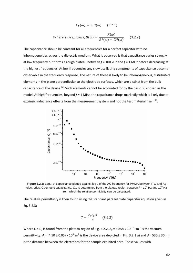
62
The capacitance should be constant for all frequencies for a perfect capacitor with no
inhomogeneities across the dielectric medium. What is observed is that capacitance varies strongly
at low frequency but forms a rough plateau between f = 100 kHz and f = 1 MHz before decreasing at
the highest frequencies. At low frequencies any slow oscillating components of capacitance become
observable in the frequency response. The nature of these is likely to be inhomogeneous, distributed
elements in the plane perpendicular to the electrode surfaces, which are distinct from the bulk
capacitance of the device [5]. Such elements cannot be accounted for by the basic EC chosen as the
model. At high frequencies, beyond f = 1 MHz, the capacitance drops markedly which is likely due to
extrinsic inductance effects from the measurement system and not the test material itself [6].
Figure 3.2.2: Log10 of capacitance plotted against log10 of the AC frequency for PMMA between ITO and Ag
electrodes. Geometric capacitance, C1, is determined from the plateau region between f = 105 Hz and 10
6 Hz
from which the relative permittivity can be calculated.
The relative permittivity is then found using the standard parallel plate capacitor equation given in
Eq. 3.2.3:
Where C = C1 is found from the plateau region of Fig. 3.2.2, ε0 = 8.854 x 10⁻¹² Fm-1 is the vacuum
permittivity, A = (4.50 ± 0.05) x 10-6 m2 is the device area depicted in Fig. 3.2.1 a) and d = 530 ± 30nm
is the distance between the electrodes for the sample exhibited here. These values with
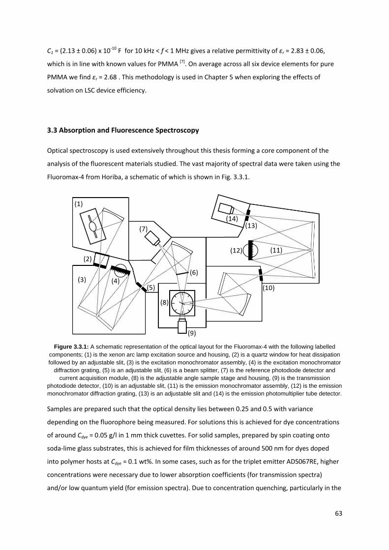
63
C1 = (2.13 ± 0.06) x 10-10 F for 10 kHz < f < 1 MHz gives a relative permittivity of εr = 2.83 ± 0.06,
which is in line with known values for PMMA [7]. On average across all six device elements for pure
PMMA we find εr = 2.68 . This methodology is used in Chapter 5 when exploring the effects of
solvation on LSC device efficiency.
3.3 Absorption and Fluorescence Spectroscopy
Optical spectroscopy is used extensively throughout this thesis forming a core component of the
analysis of the fluorescent materials studied. The vast majority of spectral data were taken using the
Fluoromax-4 from Horiba, a schematic of which is shown in Fig. 3.3.1.
Figure 3.3.1: A schematic representation of the optical layout for the Fluoromax-4 with the following labelled
components; (1) is the xenon arc lamp excitation source and housing, (2) is a quartz window for heat dissipation
followed by an adjustable slit, (3) is the excitation monochromator assembly, (4) is the excitation monochromator
diffraction grating, (5) is an adjustable slit, (6) is a beam splitter, (7) is the reference photodiode detector and
current acquisition module, (8) is the adjustable angle sample stage and housing, (9) is the transmission
photodiode detector, (10) is an adjustable slit, (11) is the emission monochromator assembly, (12) is the emission
monochromator diffraction grating, (13) is an adjustable slit and (14) is the emission photomultiplier tube detector.
Samples are prepared such that the optical density lies between 0.25 and 0.5 with variance
depending on the fluorophore being measured. For solutions this is achieved for dye concentrations
of around Cdye = 0.05 g/l in 1 mm thick cuvettes. For solid samples, prepared by spin coating onto
soda-lime glass substrates, this is achieved for film thicknesses of around 500 nm for dyes doped
into polymer hosts at Cdye = 0.1 wt%. In some cases, such as for the triplet emitter ADS067RE, higher
concentrations were necessary due to lower absorption coefficients (for transmission spectra)
and/or low quantum yield (for emission spectra). Due to concentration quenching, particularly in the

64
solid state, increasing concentration may not improve the signal in emission spectra and so either
thicker samples or adjustment of the monochromator slit widths (see Fig. 3.3.1) is the best
approach. In general alteration of the doping concentration is avoided for the above reason and
because self-solvation effects can result in emission spectrum shifts as a function of concentration
for fluorophores whose dipole moment changes upon excitation.
Absorption spectroscopy utilises the transmission detector, (9) in Fig. 3.3.1, with the sample
positioned normal to the path of the excitation source. Transmission spectra for both the blank
substrate, T0(λ), and the sample, T1(λ), are taken so that subtraction of the substrate absorption
contribution can be performed. These are first corrected by division by the reference spectrum, (7)
in Fig. 4.3.1, to remove the xenon lamp spectrum from the measured transmission. The transmission
and reference spectra are measured in μA and therefore division also normalises the units. Slit
widths equivalent of a 1 nm bandpass (0.235 mm slit width) are used for the excitation
monochromator ((3) in Fig. 3.3.1). The absorption spectrum of the test fluorophore, Sabs(λ), is then
found by Eq. (3.3.1):
The units are intensity relative to the excitation source and Sabs(λ) is generally normalised by its
maximum value to avoid ambiguity. The act of using a blank substrate introduces a systematic error
due to differences in reflectivity at the interfaces. Essentially there are two reflections for a blank
substrate and one for an optically dense sample. Using the Fresnel equations given by Eqs. (2.2.2)
and (2.2.3), with n2 = 1.52 for a typical crown glass [8] (such as borosilicate glass), this gives an error
on the absorption of 4.3% which needs to be corrected. Not doing so can result in negative
absorption.
From the transmission data it is also possible to determine the absorption and extinction coefficients
for a given fluorophore using the Beer-Lambert law as defined by Eq. (2.2.5). The transmission
spectrum as a result purely of the absorption due to the fluorophore is given by the ratio T1(λ)/ T0(λ)
which is equivalent to the intensity ratio I(λ)/I0(λ) and hence the extinction coefficient can be shown
to be;
Where Cdye is the molar dye concentration and <x> is the mean film thickness measured by
profilometry.
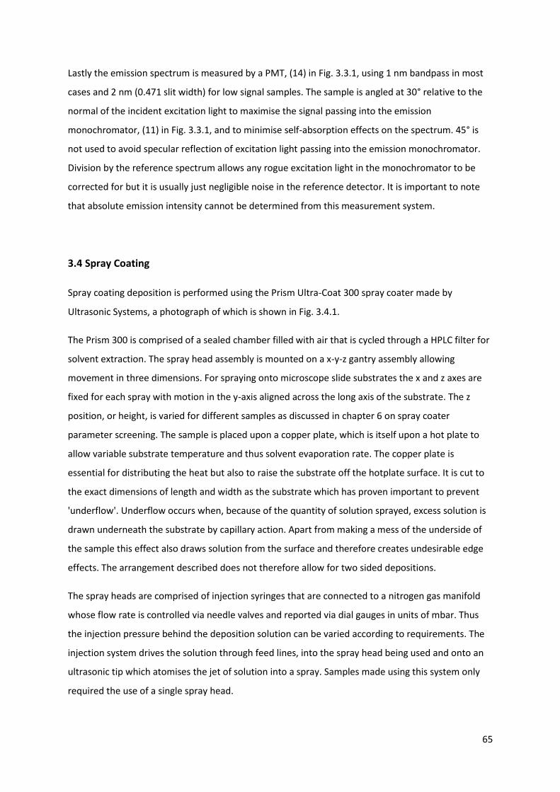
65
Lastly the emission spectrum is measured by a PMT, (14) in Fig. 3.3.1, using 1 nm bandpass in most
cases and 2 nm (0.471 slit width) for low signal samples. The sample is angled at 30° relative to the
normal of the incident excitation light to maximise the signal passing into the emission
monochromator, (11) in Fig. 3.3.1, and to minimise self-absorption effects on the spectrum. 45° is
not used to avoid specular reflection of excitation light passing into the emission monochromator.
Division by the reference spectrum allows any rogue excitation light in the monochromator to be
corrected for but it is usually just negligible noise in the reference detector. It is important to note
that absolute emission intensity cannot be determined from this measurement system.
3.4 Spray Coating
Spray coating deposition is performed using the Prism Ultra-Coat 300 spray coater made by
Ultrasonic Systems, a photograph of which is shown in Fig. 3.4.1.
The Prism 300 is comprised of a sealed chamber filled with air that is cycled through a HPLC filter for
solvent extraction. The spray head assembly is mounted on a x-y-z gantry assembly allowing
movement in three dimensions. For spraying onto microscope slide substrates the x and z axes are
fixed for each spray with motion in the y-axis aligned across the long axis of the substrate. The z
position, or height, is varied for different samples as discussed in chapter 6 on spray coater
parameter screening. The sample is placed upon a copper plate, which is itself upon a hot plate to
allow variable substrate temperature and thus solvent evaporation rate. The copper plate is
essential for distributing the heat but also to raise the substrate off the hotplate surface. It is cut to
the exact dimensions of length and width as the substrate which has proven important to prevent
'underflow'. Underflow occurs when, because of the quantity of solution sprayed, excess solution is
drawn underneath the substrate by capillary action. Apart from making a mess of the underside of
the sample this effect also draws solution from the surface and therefore creates undesirable edge
effects. The arrangement described does not therefore allow for two sided depositions.
The spray heads are comprised of injection syringes that are connected to a nitrogen gas manifold
whose flow rate is controlled via needle valves and reported via dial gauges in units of mbar. Thus
the injection pressure behind the deposition solution can be varied according to requirements. The
injection system drives the solution through feed lines, into the spray head being used and onto an
ultrasonic tip which atomises the jet of solution into a spray. Samples made using this system only
required the use of a single spray head.
66
Figure 3.4.1: Annotated photograph of the Prism 300 spray coater showing the x-y-z gantry assembly, spray
head assembly, hotplate and a finished sample on a copper plate. The upright syringes at centre contain only
isopropanol here as no depositions are being performed. Syringe A, at the image's centre, is used here passing
deposition material via the clear white feed line, through an electronically controlled valve and down to the
ultrasonic tip of the spray head.
3.5 Time Correlated Single Photon Counting (TCSPC)
A useful optical property to measure for fluorescent materials is the fluorescence lifetime, τ, which is
typically measured using Time Correlated Single Photon Counting (TCSPC) [9]. As seen in Eq. (2.4.1)
this measured lifetime can be used in conjunction with fluorescence quantum yield measurements,
described above in 3.1, to begin to understand the balance between radiative and non-radiative
transitions. This lends these complimentary measurements towards appreciation and quantification
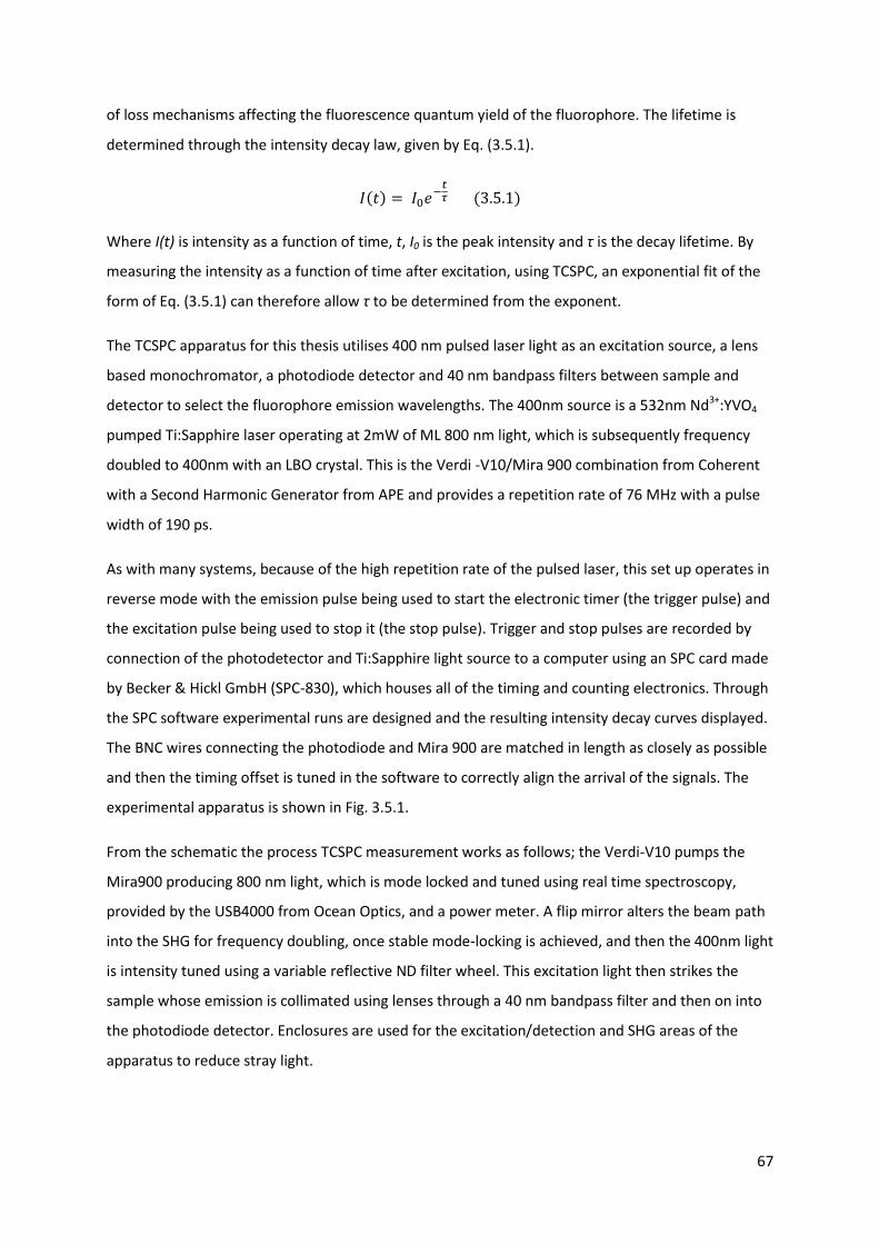
67
of loss mechanisms affecting the fluorescence quantum yield of the fluorophore. The lifetime is
determined through the intensity decay law, given by Eq. (3.5.1).
Where I(t) is intensity as a function of time, t, I0 is the peak intensity and τ is the decay lifetime. By
measuring the intensity as a function of time after excitation, using TCSPC, an exponential fit of the
form of Eq. (3.5.1) can therefore allow τ to be determined from the exponent.
The TCSPC apparatus for this thesis utilises 400 nm pulsed laser light as an excitation source, a lens
based monochromator, a photodiode detector and 40 nm bandpass filters between sample and
detector to select the fluorophore emission wavelengths. The 400nm source is a 532nm Nd3+:YVO4
pumped Ti:Sapphire laser operating at 2mW of ML 800 nm light, which is subsequently frequency
doubled to 400nm with an LBO crystal. This is the Verdi -V10/Mira 900 combination from Coherent
with a Second Harmonic Generator from APE and provides a repetition rate of 76 MHz with a pulse
width of 190 ps.
As with many systems, because of the high repetition rate of the pulsed laser, this set up operates in
reverse mode with the emission pulse being used to start the electronic timer (the trigger pulse) and
the excitation pulse being used to stop it (the stop pulse). Trigger and stop pulses are recorded by
connection of the photodetector and Ti:Sapphire light source to a computer using an SPC card made
by Becker & Hickl GmbH (SPC-830), which houses all of the timing and counting electronics. Through
the SPC software experimental runs are designed and the resulting intensity decay curves displayed.
The BNC wires connecting the photodiode and Mira 900 are matched in length as closely as possible
and then the timing offset is tuned in the software to correctly align the arrival of the signals. The
experimental apparatus is shown in Fig. 3.5.1.
From the schematic the process TCSPC measurement works as follows; the Verdi-V10 pumps the
Mira900 producing 800 nm light, which is mode locked and tuned using real time spectroscopy,
provided by the USB4000 from Ocean Optics, and a power meter. A flip mirror alters the beam path
into the SHG for frequency doubling, once stable mode-locking is achieved, and then the 400nm light
is intensity tuned using a variable reflective ND filter wheel. This excitation light then strikes the
sample whose emission is collimated using lenses through a 40 nm bandpass filter and then on into
the photodiode detector. Enclosures are used for the excitation/detection and SHG areas of the
apparatus to reduce stray light.
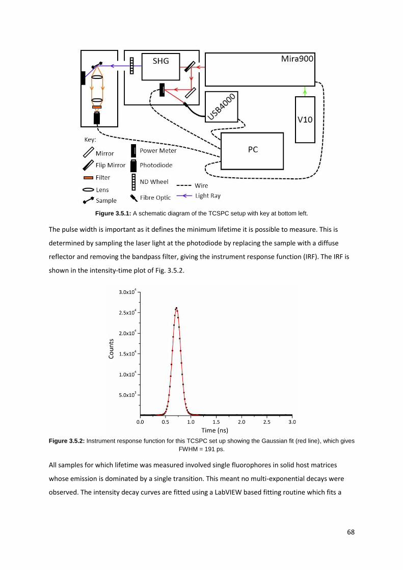
68
Figure 3.5.1: A schematic diagram of the TCSPC setup with key at bottom left.
The pulse width is important as it defines the minimum lifetime it is possible to measure. This is
determined by sampling the laser light at the photodiode by replacing the sample with a diffuse
reflector and removing the bandpass filter, giving the instrument response function (IRF). The IRF is
shown in the intensity-time plot of Fig. 3.5.2.
Figure 3.5.2: Instrument response function for this TCSPC set up showing the Gaussian fit (red line), which gives
FWHM = 191 ps.
All samples for which lifetime was measured involved single fluorophores in solid host matrices
whose emission is dominated by a single transition. This meant no multi-exponential decays were
observed. The intensity decay curves are fitted using a LabVIEW based fitting routine which fits a
69
single exponential decay function to the data across an appropriate interval. The fitted function thus
provides the lifetime.
3.6 Spin Coating
The fabrication of thin films for spectroscopic study is typically done by spin coating using a Laurell
ws-400bz-6npp/lite spin coater. Such tools are not suited to large area thin film coverage but offer
advantage in producing samples quickly and cheaply, relative to more sophisticated techniques such
as spray coating. Samples produced by this method are typically used in various optical
measurements such as quantum yield, fluorescence lifetime, emission spectra and absorption
coefficients. A disadvantage of spin coaters is that the film edges tend to be thicker than the middle
as surface tension draws material outwards during fabrication. Total solution concentration strongly
affects the resultant thin film thickness, which must be optimised through profilometry (section 3.8)
on trial samples to get the desired thickness for a given concentration.
To spin coat a thin film a polymer, which may be a light emitting polymer (chapter 2.4.2) or a optical
host (chapter 2.4.3), is first dissolved in a suitable solvent in a sealed vial. If a optical host is used
then the host solution is blended with a small molecular fluorophore in the same solvent, or one
miscible with the other, to achieve the desired fluorophore concentration. Next a small glass
substrate, 1.5 x 1 cm, is placed on the spin coater chuck over a source of vacuum. The substrate is
fixed by the vacuum and a rubber o-ring is used to make a seal. Usually the spin coater is set running
at the required rpm and then thin films are deposited from solution by a micro-pipette onto the
spinning substrate. However, high concentrations of host polymer (>150 g/l) result in high viscosities
that require some spreading time prior to starting the spin coater, otherwise full coverage is not
achieved.
3.7 Profilometry
Profilometry is performed to measure thin film thickness and roughness throughout this thesis using
a Veeco DekTak 150, which is a contact profilometer. The device uses a mechanically controlled
stylus, operated by software, which is lowered onto the sample surface until it exerts between 0.03
and 50 mg of force; typically 30 mg is used. The sample is mounted on a xy stage which is tracked
when performing a scan so that the sample surface moves under the tip of the stylus. Scan ranges of

70
up to 10 mm are possible. A camera is used for positioning the start of the scan and to observe the
surface features of the sample.
To measure thin film thickness a groove is cut through the thin film using a pair of tweezers, taking
care not to scratch the glass underneath, and a scan is made across this groove. Scratching the glass
would artificially increase the film thickness so blunter tweezers are preferable for this operation.
From the resultant profile a clear step can be seen and the film thickness estimated to an accuracy of
±10 nm through several measurements per sample.
When measuring surface roughness carving a groove in the thin film is not necessary and a long scan
is performed over the thin film surface. The profile scan is recorded to a computer for analysis
including levelling of the profile and performing a peak detector analysis. This is done exclusively and
explained in more detail in chapter 6. Long scan times are generally used to increase the accuracy of
the measurement.
71
3.8 References
[1] A. R. Johnson, S. Lee, J. Klein and J. Kanicki, Absolute photoluminescence quantum efficiency
measurement of light-emitting thin films, Rev. Sci. Instrum. 78, 096101 (2007)
[2] T. Ahn, R. O. Al-Kaysi, A. M. Müller, K. M. Wentz and C. J. Bardeen, Self-absorption correction for
solid-state photoluminescence quantum yields obtained from integrating sphere measurements,
Rev. Sci. Instrum. 78, 086105 (2007)
[3] J. C. de Mello, H. F. Wittmann and R. H. Friend, An improved experimental determination of
external photoluminescence quantum efficiency, Adv. Mater. 9, 3 (1997)
[4] N. C. Greenham, I. D. W. Samuel, G. R. Hayes, R. T. Phillips, Y. A. R. R. Kessener, S. C. Moratti, A. B.
Holmes and R. H. Friend, Measurement of absolute photoluminescence quantum efficiencies in
conjugated polymers, Chem. Phys. Lett. 241, 89 (1995)
[5] E. Barsoukov and J. R. Macdonald, Impedance Spectroscopy Theory, Experiment, and
Applications, Wiley-Interscience, Chap. 1 + 2, 1 - 42 (2005)
[6] M. Li, D. C. Sinclair and A. R. West, Extrinsic origins of the apparent relaxorlike behavior in
CaCu3Ti4O12 ceramics at high temperatures: A cautionary tale, J. App. Phys. 102, 084106 (2011)
[7] Computer Support Group (CSG) Inc., (1973 - 2013)
http://www.csgnetwork.com/dieconstantstable.html
[8] C. R. Nave, Hyper Physics, Georgia State University (2012)
http://hyperphysics.phy-astr.gsu.edu/hbase/tables/indrf.html
[9] W. Becker, The bh TCSPC Handbook, 5th Ed., Becker & Hickl GmbH (2012)
72
Chapter 4
Rigorous Measurement of Quantum Yield Using the Gauge R & R
Methodology
4.1 Introduction
This chapter explores sources of uncertainty in an integration sphere based measurement of
fluorescence quantum yield of solid state systems, ηQY [1]. For LSC devices, achieving a high ηQY of the
luminescent materials is of critical importance to the overall optical efficiency, ηopt, as per Eq. 2.2.15.
After the absorption of incident solar energy this is the next loss mechanism physically imposed on a
LSC device. It is therefore important to be able to make accurate measurements of ηQY in order to
make useful experimental studies of LSCs.
The assessment methodology employed here discriminates between variance in the sample, day to
day variation and the measurement system. Measurement of ηQY is complex and involves multiple
sources of uncertainty including wavelength sensitivity characterisation using a calibration light
source, self-absorption corrections by spectral methods, sample variance and laser intensity
variance. These sources of uncertainty pose significant challenges that need addressing to improve
the absolute measurement technique using the integration sphere. However, alternative methods of
ηQY determination, which include the relative method and the thermal lens technique, pose greater
challenges. The relative method relies on comparison of the subject fluorophore to a known
standard, such as R6G or quinine sulphate, which contains large uncertainty from achieving the
correct experimental conditions for the standard and, particularly for solid state systems, in emission
anisotropy effects. The thermal lens technique is a purportedly more accurate absolute method but
has been seen to be fraught with technical difficulties [2].
Assessment of the integration sphere method is performed using a statistical approach employed in
industry for reliable characterisation of measurement gauges in manufacturing. This approach is
used to set tolerances on production processes and gives insight into the sources of variance in the
manufacturing industry. The method is known as Gauge R&R (GRR). The “Gauge” is the
measurement device which may be a ruler, micrometre or, as in this case, a multi-component
system with many potential sources of error. The R&R stands for Repeatability and Reproducibility,
which relate to the measurement equipment and operative respectively. The GRR method is
73
demonstrated here to have value in characterising scientific instruments and is described in detail
through the section 4.2. In 4.3 experimental methods are discussed providing additional details to
those given in chapter 3.1. In section 4.4 the results of the study are explored and discussed in
detail. Section 4.5 concludes on the findings of this study.
4.2 The Gauge R & R Methodology
The GRR method presented here is based on D. Wheeler's formulation of the study design [3], which
corrects for mathematical inconsistencies in the standard Automotive Industry Action Group (AIAG)
formulation. This statistical method allows sources of variance to be ascertained in three groupings;
Equipment Variation (EV), Appraiser Variation (AV) and Manufacturing Variation (MV). The three
sources of variation reflect the different aspects of the experiment and the production process. The
EV relates to the measurement system, the AV relates to the appraiser, or operative, and the MV,
also called product variation, relates to sample fabrication. In this study there is only one operative
and so the appraiser variation is instead a day-to-day variation. On each day the components of the
ηQY measurement system are removed and then reconnected and the laser is warmed up and tuned.
Suffice to say this variance no longer represents that of an AV from a traditional GRR but will instead
give indication of a variance associated with setting up and calibrating the experiment. Since this is
essentially an equipment variation it is reasonable to expect it to be of roughly the same magnitude
as the actual EV.
The essential requirement a GRR study is to have a fully crossed data structure, such that a full
coverage of the permutations of variables is achieved. The variables here are n, o and p which are
the number of repeat measurements per sample, number of days over which the study was
performed and the number of samples, respectively. The measured parameter is the quantum yield,
but the data structure of the GRR study is based on values the quantum yield takes for the variables
n, o and p. Thus by a fully-crossed data structure what is meant is that all permutations of n, o and p
have an associated quantum yield measurement, which creates the basis of the GRR statistical
analysis.
This experiment is set for three measurements per sample over three days on five different samples,
per material, and hence n = 3, o = 3 and p = 5. So there are k = op = 15 subgroups, each of size n = 3.
The first step is to take the average range of the k subgroups of size n = 3, which each have a
range, R. Then the Upper Range Limit, RURL , is determined using Eq. (4.2.1);
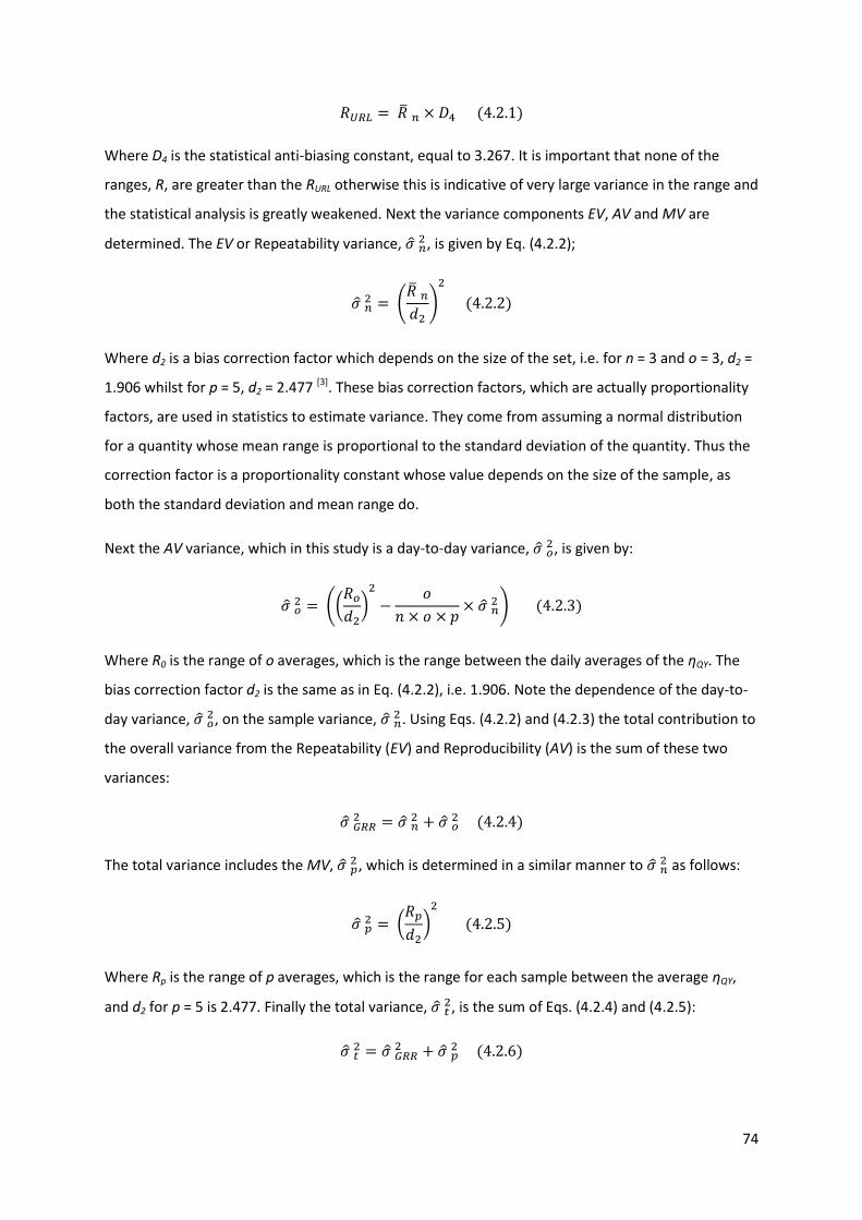
74
Where D4 is the statistical anti-biasing constant, equal to 3.267. It is important that none of the
ranges, R, are greater than the RURL otherwise this is indicative of very large variance in the range and
the statistical analysis is greatly weakened. Next the variance components EV, AV and MV are
determined. The EV or Repeatability variance, , is given by Eq. (4.2.2);
Where d2 is a bias correction factor which depends on the size of the set, i.e. for n = 3 and o = 3, d2 =
1.906 whilst for p = 5, d2 = 2.477 [3]. These bias correction factors, which are actually proportionality
factors, are used in statistics to estimate variance. They come from assuming a normal distribution
for a quantity whose mean range is proportional to the standard deviation of the quantity. Thus the
correction factor is a proportionality constant whose value depends on the size of the sample, as
both the standard deviation and mean range do.
Next the AV variance, which in this study is a day-to-day variance, , is given by:
Where R0 is the range of o averages, which is the range between the daily averages of the ηQY. The
bias correction factor d2 is the same as in Eq. (4.2.2), i.e. 1.906. Note the dependence of the day-to-
day variance, , on the sample variance,
. Using Eqs. (4.2.2) and (4.2.3) the total contribution to
the overall variance from the Repeatability (EV) and Reproducibility (AV) is the sum of these two
variances:
The total variance includes the MV, , which is determined in a similar manner to
as follows:
Where Rp is the range of p averages, which is the range for each sample between the average ηQY,
and d2 for p = 5 is 2.477. Finally the total variance, , is the sum of Eqs. (4.2.4) and (4.2.5):
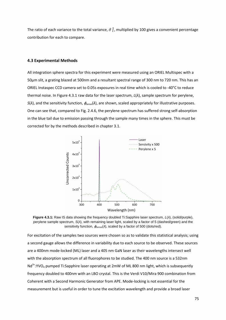
75
The ratio of each variance to the total variance, , multiplied by 100 gives a convenient percentage
contribution for each to compare.
4.3 Experimental Methods
All integration sphere spectra for this experiment were measured using an ORIEL Multispec with a
50µm slit, a grating blazed at 500nm and a resultant spectral range of 300 nm to 720 nm. This has an
ORIEL Instaspec CCD camera set to 0.05s exposures in real time which is cooled to -40°C to reduce
thermal noise. In Figure 4.3.1 raw data for the laser spectrum, L(λ), sample spectrum for perylene,
S(λ), and the sensitivity function, φsense(λ), are shown, scaled appropriately for illustrative purposes.
One can see that, compared to Fig. 2.4.6, the perylene spectrum has suffered strong self-absorption
in the blue tail due to emission passing through the sample many times in the sphere. This must be
corrected for by the methods described in chapter 3.1.
Figure 4.3.1: Raw IS data showing the frequency doubled Ti:Sapphire laser spectrum, L(λ), (solid/purple),
perylene sample spectrum, S(λ), with remaining laser light, scaled by a factor of 5 (dashed/green) and the
sensitivity function, φsense(λ), scaled by a factor of 500 (dots/red).
For excitation of the samples two sources were chosen so as to validate this statistical analysis; using
a second gauge allows the difference in variability due to each source to be observed. These sources
are a 400nm mode-locked (ML) laser and a 405 nm GaN laser as their wavelengths intersect well
with the absorption spectrum of all fluorophores to be studied. The 400 nm source is a 532nm
Nd3+:YVO4 pumped Ti:Sapphire laser operating at 2mW of ML 800 nm light, which is subsequently
frequency doubled to 400nm with an LBO crystal. This is the Verdi V10/Mira 900 combination from
Coherent with a Second Harmonic Generator from APE. Mode-locking is not essential for the
measurement but is useful in order to tune the excitation wavelength and provide a broad laser
76
spectrum that is more distributed over the CCD detection array. This avoids CCD saturation and
provides greater dynamic range between the laser and sample emission integration as discussed
subsequently. While mode-locking generates a significantly higher instantaneous power than an
equivalent average power continuous wave (CW) laser, the fluorescence lifetime of the materials
ranges between 200 ps (F8) to 5 ns (Perylene) and therefore the system behaves in a quasi-
continuous way when pulse periods are around 12 ns as in the Ti:Sapphire cavity. We have ensured
that all our experimental systems behave linearly by measuring the ηQY at different excitation
densities. No change in ηQY as a function of excitation density was observed but nevertheless
excitation power was kept as low as possible. The 405 nm laser is a GaN diode laser which operates
in CW mode, provides a steady mW of power and has a larger spot size than the ML laser which
lowers energy density.
Five identical samples of each of three materials were fabricated and measured according to the
Gauge R & R methodology. Blue-emitting conjugated polymer poly(9,9-dioctylfluorene) (F8) was
provided by CDT, blue-green perylene dye was purchased from Sigma Aldrich and red-emitting
perylene derivative perylene red (PR) was provided by BASF. F8 was spin coated from a 2.5 g/l
solution in toluene at 500rpm in air and then dried on a hotplate at 50°C for 5 minutes to remove all
the solvent. The resulting film thickness, measured on a Veeco DekTak, was 28±5 nm. Perylene and
PR were first dissolved in toluene at 2 g/l and then blended with a solution of poly(methyl
methacrylate) (PMMA) in toluene at 250 g/l in a 1:24 (dye:PMMA w/w) ratio giving a resultant dye
concentration of 0.5% by weight. This corresponds to 2.36x10⁻² M and 6.17x10⁻³ M for perylene and
PR respectively. The perylene and PR samples are then prepared by spin coating the blends at
1500rpm in air and then dried on a hotplate at 50°C for 5 minutes. Resultant film thicknesses vary
between 4.5 and 5.5 µm.
These choices were made for this study because F8 provides a known standard with well explored
properties and because the perylene dyes are a promising material class for molecular dye based LSC
devices. In a paper by A. J. Cadby et. al. the ηQY of F8 was found to be 45 ± 5 %, under different
processing conditions to those used here [4]. Previously, for perylene and PR, ηQY values have been
found ranging between 86 ± 2 % and 63 ± 2 % at concentrations of 0.1 %wt and 1 %wt (4.68x10⁻³ M
and 4.73x10⁻² M) for perylene and ηQY between 68 ± 2 % and 46 ± 2 % at concentrations of 0.1 %wt
and 1.5 %wt (1.22x10⁻³ M and 1.86x10⁻² M) for PR. These values for Perylene are in contradiction to
that used by S. Lee et. al. (2006) [5], which was ηQY = 94% at a concentration of 0.1070 M. They do not
explain how this value was determined, however. Further, the values found here for PR contradict
those measured by Fennel and Lochbrunner (2011) [6] who found ηQY = 81 % at a concentration of
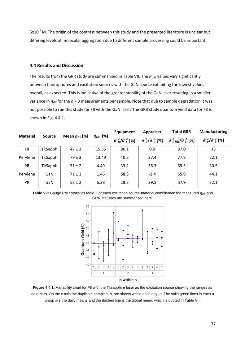
77
5x10⁻² M. The origin of the contrast between this study and the presented literature is unclear but
differing levels of molecular aggregation due to different sample processing could be important.
4.4 Results and Discussion
The results from the GRR study are summarised in Table VII. The RURL values vary significantly
between fluorophores and excitation sources with the GaN source exhibiting the lowest values
overall, as expected. This is indicative of the greater stability of the GaN laser resulting in a smaller
variance in ηQY for the n = 3 measurements per sample. Note that due to sample degradation it was
not possible to run this study for F8 with the GaN laser. The GRR study quantum yield data for F8 is
shown in Fig. 4.4.1.
Material Source Mean ηQY [%] RURL [%] Equipment
/
[%]
Appraiser
/
[%]
Total GRR
/
[%]
Manufacturing
/
[%]
F8 Ti:Sapph 47 ± 3 15.35 86.1 0.9 87.0 13
Perylene Ti:Sapph 79 ± 3 13.49 40.5 37.4 77.9 22.1
PR Ti:Sapph 51 ± 2 4.49 33.2 36.3 69.5 30.5
Perylene GaN 71 ± 1 1.46 58.3 -2.4 55.9 44.1
PR GaN 53 ± 2 6.28 28.3 39.5 67.9 32.1
Table VII: Gauge R&R statistics table. For each excitation source-material combination the measured ηQY and
GRR statistics are summarised here.
Figure 4.4.1: Variability chart for F8 with the Ti:sapphire laser as the excitation source showing the ranges as
data bars. On the x-axis the duplicate samples, p, are shown within each day, o. The solid green lines in each o
group are the daily means and the dashed line is the global mean, which is quoted in Table VII.

78
The mean ηQY is given here as a percentage, notice in Table VII that the yield measured for perylene
is different for the two excitation sources. The reason for this is unclear as this difference is not
reflected in the values for PR and photoluminescence excitation measurements indicate no dark
states are present for perylene. None-the-less this discrepancy was observed consistently across the
study in perylene's case, which can be seen in the variability charts for perylene in Fig. 4.4.2. The fact
that ηQY is higher for the Ti:sapphire laser rules out the possibility of quenching due to higher exciton
densities. Despite this conundrum the GRR study's validity is not affected with respect to
ascertaining sources of variability.
Looking at the GRR statistics in Table VII for the Ti:sapphire laser both perylene and PR show a level
of balance between the equipment and appraiser variances as is expected. This trend is not carried
for F8 as in this case the variance between the n = 3 measurements per sample dominated over the
AV component. Looking at Fig. 4.4.1 we can see this in the large fluctuations in individual points
relative to o group means, in other words large ranges reflected by the RURL. Also note the very low
manufacturing variance, which indicates a high production tolerance from part to part for F8. This
suggests greater homogeneity across the sample surface relative to the PMMA:dye systems.
The values for MV are in all cases below 50% designating this measurement system as a third-class
monitor in Gauge R & R terminology. This means that the dominant source of variance lies in the
measurement apparatus and not the sample production. We can see from the MV values that
employing the GaN laser reduces the dominance of the measurement apparatus variance to some
extent.
Some sample irregularities are expected and present but they have the smallest influence. Such
irregularities will consist of point to point variations in thickness or fluorophore density across the
sample films. It would be expected that the small molecules, perylene and PR, doped into PMMA
would exhibit this more strongly and indeed the MV is lowest for F8, which is the thinnest film and
of a single, pure material. Sample inconsistencies translated to a full LSC device are certainly
undesirable though probably a relative minor factor compared to other loss mechanisms.
This sample irregularity combined with small oscillations in the intensity of the laser results in the
distribution seen in ηQY. With this experimental setup it is not possible to know the exact number of
laser counts at the time of each measurement. Instead a series of laser spectra are taken, as
described in Chapter 3.1, between each sample measurement from which an average laser profile is
used for all ηQY determinations.

79
The fact that the GRR (EV + AV) component dominates over MV, and thus most error lies in the
equipment, does not itself say the measurement system is inaccurate. The GRR statistics only
indicate that one source of variance is larger than another, saying nothing therefore of absolute
uncertainties. To find the true uncertainties we multiply the GRR and MV variances as ratios by the
uncertainty in ηQY for each material and source. Through this the greater stability of the GaN laser is
seen by comparing the uncertainties. The results of this are shown in Table VIII.
To further explore the GRR data in Figures 4.4.2 and 4.4.3 are the variability charts for perylene and
PR using the two excitation sources. It is immediately obvious that, for particular samples, there is
little or no correlation between ηQY values over different days, o. In other words, few samples have
consistent values throughout the study. No pattern of declining yields due to photobleaching or
other chemically destructive reactions are observed and these samples were stored in air. PMMA
acts a significant barrier to quenching agents such as molecular oxygen or moisture.
Material Source ΔηQY [%] Total GRR
/
Manufacturing
/
ΔGRR [%] ΔMV [%]
F8 Ti:Sapph ±3 0.87 0.13 ±2.61 ±0.39
Perylene Ti:Sapph ±3 0.779 0.221 ±2.34 ±0.66
PR Ti:Sapph ±2 0.695 0.305 ±1.39 ±0.61
Perylene GaN ±1 0.559 0.441 ±0.56 ±0.44
PR GaN ±2 0.679 0.321 ±1.36 ±0.64
Table VIII: Gauge R&R uncertainties; the contributions from GRR and MV variances to the total uncertainty are
summarised here
Figure 4.4.2: Variability charts for perylene; on the left using the Ti:Sapphire laser and on the right using the GaN
laser.
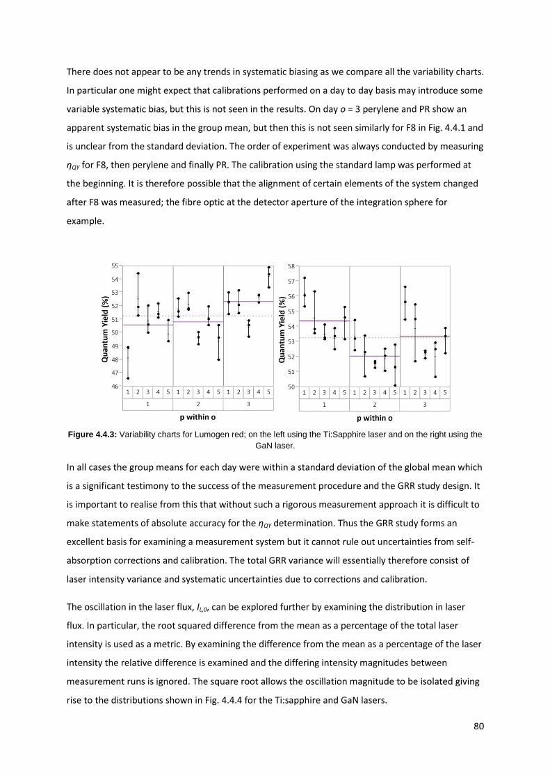
80
There does not appear to be any trends in systematic biasing as we compare all the variability charts.
In particular one might expect that calibrations performed on a day to day basis may introduce some
variable systematic bias, but this is not seen in the results. On day o = 3 perylene and PR show an
apparent systematic bias in the group mean, but then this is not seen similarly for F8 in Fig. 4.4.1 and
is unclear from the standard deviation. The order of experiment was always conducted by measuring
ηQY for F8, then perylene and finally PR. The calibration using the standard lamp was performed at
the beginning. It is therefore possible that the alignment of certain elements of the system changed
after F8 was measured; the fibre optic at the detector aperture of the integration sphere for
example.
Figure 4.4.3: Variability charts for Lumogen red; on the left using the Ti:Sapphire laser and on the right using the
GaN laser.
In all cases the group means for each day were within a standard deviation of the global mean which
is a significant testimony to the success of the measurement procedure and the GRR study design. It
is important to realise from this that without such a rigorous measurement approach it is difficult to
make statements of absolute accuracy for the ηQY determination. Thus the GRR study forms an
excellent basis for examining a measurement system but it cannot rule out uncertainties from self-
absorption corrections and calibration. The total GRR variance will essentially therefore consist of
laser intensity variance and systematic uncertainties due to corrections and calibration.
The oscillation in the laser flux, IL,0, can be explored further by examining the distribution in laser
flux. In particular, the root squared difference from the mean as a percentage of the total laser
intensity is used as a metric. By examining the difference from the mean as a percentage of the laser
intensity the relative difference is examined and the differing intensity magnitudes between
measurement runs is ignored. The square root allows the oscillation magnitude to be isolated giving
rise to the distributions shown in Fig. 4.4.4 for the Ti:sapphire and GaN lasers.
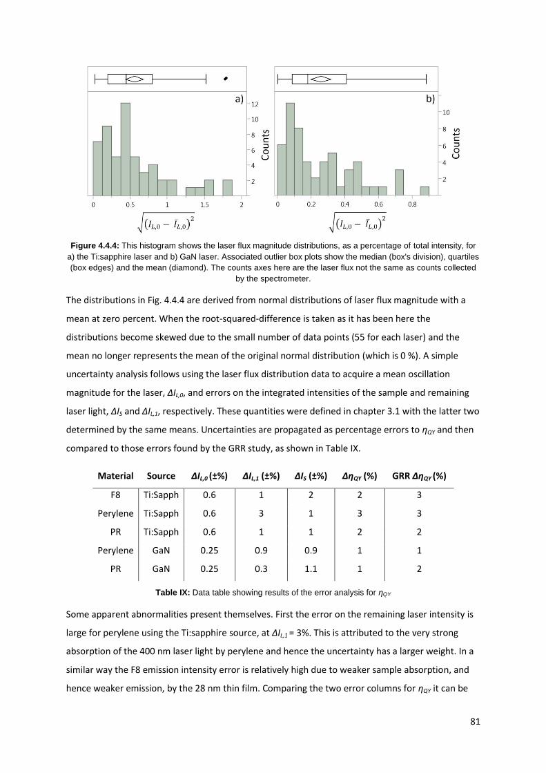
81
Figure 4.4.4: This histogram shows the laser flux magnitude distributions, as a percentage of total intensity, for
a) the Ti:sapphire laser and b) GaN laser. Associated outlier box plots show the median (box's division), quartiles
(box edges) and the mean (diamond). The counts axes here are the laser flux not the same as counts collected
by the spectrometer.
The distributions in Fig. 4.4.4 are derived from normal distributions of laser flux magnitude with a
mean at zero percent. When the root-squared-difference is taken as it has been here the
distributions become skewed due to the small number of data points (55 for each laser) and the
mean no longer represents the mean of the original normal distribution (which is 0 %). A simple
uncertainty analysis follows using the laser flux distribution data to acquire a mean oscillation
magnitude for the laser, ΔIL,0, and errors on the integrated intensities of the sample and remaining
laser light, ΔIS and ΔIL,1, respectively. These quantities were defined in chapter 3.1 with the latter two
determined by the same means. Uncertainties are propagated as percentage errors to ηQY and then
compared to those errors found by the GRR study, as shown in Table IX.
Material Source ΔIL,0 (±%) ΔIL,1 (±%) ΔIS (±%) ΔηQY (%) GRR ΔηQY (%)
F8 Ti:Sapph 0.6 1 2 2 3
Perylene Ti:Sapph 0.6 3 1 3 3
PR Ti:Sapph 0.6 1 1 2 2
Perylene GaN 0.25 0.9 0.9 1 1
PR GaN 0.25 0.3 1.1 1 2
Table IX: Data table showing results of the error analysis for ηQY
Some apparent abnormalities present themselves. First the error on the remaining laser intensity is
large for perylene using the Ti:sapphire source, at ΔIL,1 = 3%. This is attributed to the very strong
absorption of the 400 nm laser light by perylene and hence the uncertainty has a larger weight. In a
similar way the F8 emission intensity error is relatively high due to weaker sample absorption, and
hence weaker emission, by the 28 nm thin film. Comparing the two error columns for ηQY it can be

82
see that the GRR study is more conservative in that it generates larger errors. This is likely due to this
simple uncertainty analysis specifically looking at uncertainties in the intensities of source and
sample, no other factors included. What this shows is that laser flux variance appears to contribute a
substantial amount of uncertainty to ηQY. This follows from the point raised earlier that one cannot
know the exact intensity of the laser at the time of measurement using this setup. The second,
somewhat trivial point is that the GaN laser is more stable, as was obvious by observation, and thus
provides a more accurate measurement.
4.5 Conclusions
What is clear from this study is that the limit of accuracy possible with this system using the GaN
laser is around ± 1%. Such accuracy is not ideal for measurement of ηQY for systems with yields close
to unity, which is important for LSC devices where high yields are critical. This motivation requires a
better performance from the measurement system, though as can be seen at the concentrations
used neither perylene nor PR are reaching unity at these concentrations. At lower concentrations
they likely will, as has been seen for PR in PMMA [6].
To improve the experiment it is clear the laser flux variance needs a solution. Ideally it would be
useful to know the exact intensity of the laser flux at the time of measurement and so a portion of
the beam should be sampled using a beam splitter with a second photodiode. Then by correct timing
of the electronics an instantaneous measurement of sample and laser flux would be possible. This
would also remove extra steps in the analysis and speed up the measurement process into the
bargain. This work was not completed for this thesis.

83
4.6 References
[1] A. P. Green and A.R. Buckley, Application of Gauge R & R to the rigorous measurement of
quantum yield in fluorescent organic solid state systems. Rev. Sci. Instrum. 83, 073108 (2012)
[2] L. R. Wilson, Luminescent Solar Concentrators: A Study of Optical Properties, Re-absorption and
Device Optimisation, Ph.D, Edinburgh, Scotland (2010)
[3] D. J Wheeler, An Honest Gauge R&R Study, SPC press, 2006 ASQ/ASA fall technical conference,
manuscript no. 189
[4] A. J. Cadby, R. Dean, C. Elliott, R. A. L. Jones, A. M. Fox and D. G. Lidzey, Imaging the Fluorescence
Decay Lifetime of a Conjugated Polymer Blend By Using a Scanning Near-Field Optical Microscope,
Adv. Mater. 19, 107-111 (2007)
[5] S. Lee, A. M. Müller, R. Al-Kaysi and C. J. Bardeen, Using Perylene-Doped Polymer Nanotubes as
Fluorescence Sensors, Nano Letters 6, 7, 1420 - 1424 (2006)
[6] F. Fennel and S. Lochbrunner, Long distance energy transfer in a polymer matrix doped with a
perylene dye, Phys. Chem. Chem. Phys. 13, 3527-3533 (2011)
84
Chapter 5
Improving Luminescent Solar Concentrator Efficiency by Tuning
Fluorophore Emission with Solid State Solvation
5.1 Introduction
In this chapter the results of experiments looking at how the solvation mechanism can be used to
reduce self-absorption, and thus improve ηself, are discussed [1]. Towards the end of chapter 2.2 self-
absorption was discussed as a major loss mechanism and is expressed by Eq. (2.2.13) with the LSC
optical efficiency given by Eq. (2.2.15). The self-absorption loss mechanism has a significant impact
on performance over short path lengths through an LSC medium, as was shown in a study comparing
experiment results and ray-tracing model [2]. In that work square-planar devices are studied showing
that ηself and matrix losses limit the optical concentration, Copt, to a plateau at a LSC collection area of
1 m2. In other work, combining experiment and ray-tracing, nanorod fluorophores were shown to
have a Copt of nearly a factor of two greater than that for quantum dots [3]. This was attributed to the
nanorods (ηQY = 0.7) having a smaller overlap in absorption and emission, J, causing the self-
absorption efficiency to increase and hence the LSC output irradiance.
Solutions to this problem, apart from geometric considerations, are generally through maximising
the Stokes' shift and therefore minimising the overlap in absorption and emission spectra of the
fluorophore. The solvation mechanism was described theoretically in chapter 2.4 and can be
expressed using the Lippert-Mataga equation given by Eq. (2.4.2). By studying Eq. (2.4.2) it can be
seen that the variable physical parameters with which the influence of solvation can be controlled
are the host's optical properties, via Δf, and the fluorophore's dipole properties. First in this chapter,
in section 5.2, the host properties will be considered and hence ways that they might be influenced
to maximise Δf. In section 5.3 the fluorophore properties are discussed with the choices for this
study explained. In the results section of 5.4 solvation theory is used with experimental data to make
predictions of optical efficiency and of the limits to the gains possible though this phenomenon.
All samples are fabricated by first preparing a stock solutions of host materials in toluene so that
total composite host concentration Chost = 250 g/l. Blends are made with solutions of DCM, DCM2 or
DCJTB in toluene at Cdye = 2 g/l so that the blend has 0.1 wt% of dye. Deposition occurs onto glass
substrates by spin coating at 1000 rpm giving films of approximate thickness x = 500 ± 30 nm. For
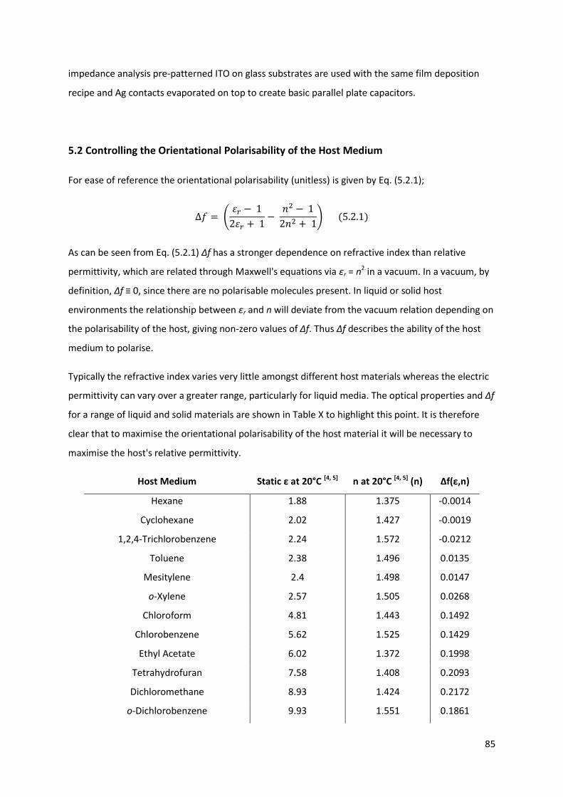
85
impedance analysis pre-patterned ITO on glass substrates are used with the same film deposition
recipe and Ag contacts evaporated on top to create basic parallel plate capacitors.
5.2 Controlling the Orientational Polarisability of the Host Medium
For ease of reference the orientational polarisability (unitless) is given by Eq. (5.2.1);
As can be seen from Eq. (5.2.1) Δf has a stronger dependence on refractive index than relative
permittivity, which are related through Maxwell's equations via εr = n2 in a vacuum. In a vacuum, by
definition, Δf ≡ 0, since there are no polarisable molecules present. In liquid or solid host
environments the relationship between εr and n will deviate from the vacuum relation depending on
the polarisability of the host, giving non-zero values of Δf. Thus Δf describes the ability of the host
medium to polarise.
Typically the refractive index varies very little amongst different host materials whereas the electric
permittivity can vary over a greater range, particularly for liquid media. The optical properties and Δf
for a range of liquid and solid materials are shown in Table X to highlight this point. It is therefore
clear that to maximise the orientational polarisability of the host material it will be necessary to
maximise the host's relative permittivity.
Host Medium Static ε at 20°C [4, 5] n at 20°C [4, 5] (n) Δf(ε,n)
Hexane 1.88 1.375 -0.0014
Cyclohexane 2.02 1.427 -0.0019
1,2,4-Trichlorobenzene 2.24 1.572 -0.0212
Toluene 2.38 1.496 0.0135
Mesitylene 2.4 1.498 0.0147
o-Xylene 2.57 1.505 0.0268
Chloroform 4.81 1.443 0.1492
Chlorobenzene 5.62 1.525 0.1429
Ethyl Acetate 6.02 1.372 0.1998
Tetrahydrofuran 7.58 1.408 0.2093
Dichloromethane 8.93 1.424 0.2172
o-Dichlorobenzene 9.93 1.551 0.1861
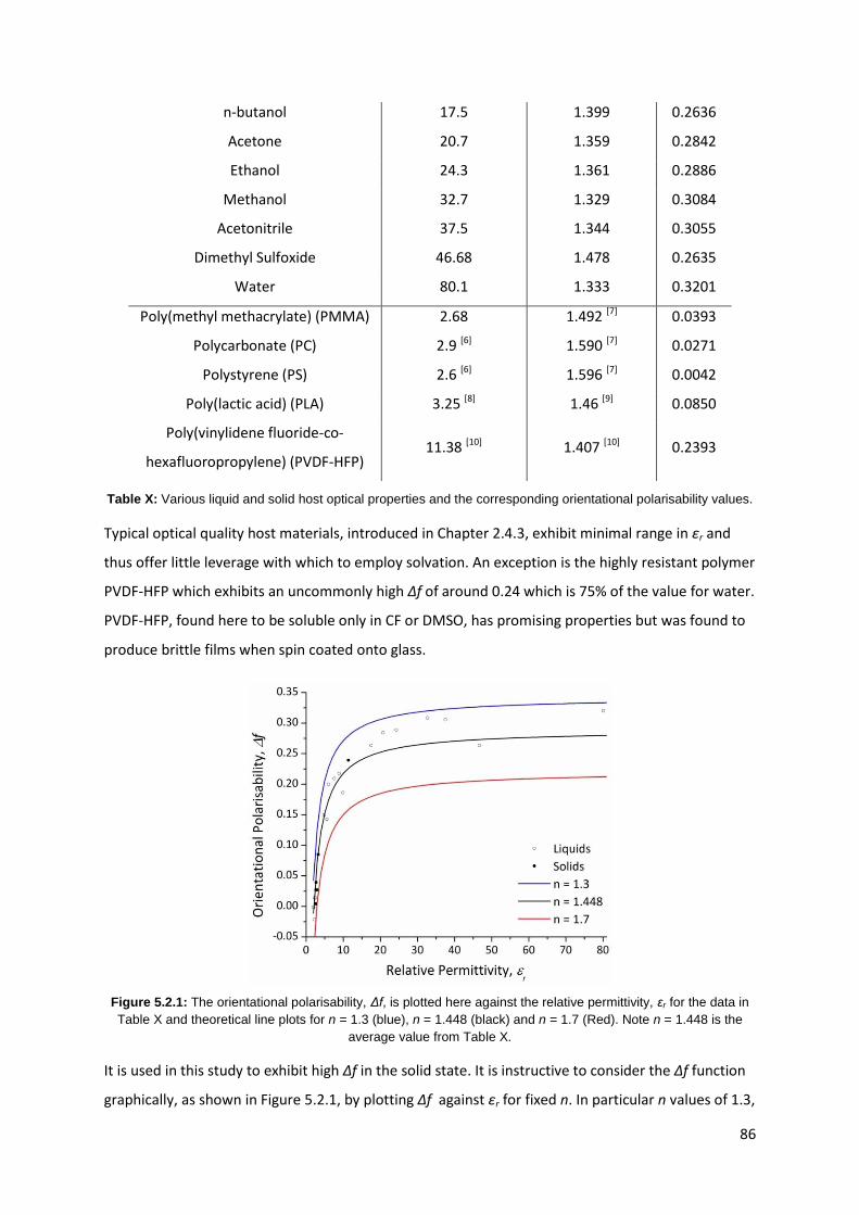
86
n-butanol 17.5 1.399 0.2636
Acetone 20.7 1.359 0.2842
Ethanol 24.3 1.361 0.2886
Methanol 32.7 1.329 0.3084
Acetonitrile 37.5 1.344 0.3055
Dimethyl Sulfoxide 46.68 1.478 0.2635
Water 80.1 1.333 0.3201
Poly(methyl methacrylate) (PMMA) 2.68 1.492 [7] 0.0393
Polycarbonate (PC) 2.9 [6] 1.590 [7] 0.0271
Polystyrene (PS) 2.6 [6] 1.596 [7] 0.0042
Poly(lactic acid) (PLA) 3.25 [8] 1.46 [9] 0.0850
Poly(vinylidene fluoride-co-
hexafluoropropylene) (PVDF-HFP) 11.38 [10] 1.407 [10] 0.2393
Table X: Various liquid and solid host optical properties and the corresponding orientational polarisability values.
Typical optical quality host materials, introduced in Chapter 2.4.3, exhibit minimal range in εr and
thus offer little leverage with which to employ solvation. An exception is the highly resistant polymer
PVDF-HFP which exhibits an uncommonly high Δf of around 0.24 which is 75% of the value for water.
PVDF-HFP, found here to be soluble only in CF or DMSO, has promising properties but was found to
produce brittle films when spin coated onto glass.
Figure 5.2.1: The orientational polarisability, Δf, is plotted here against the relative permittivity, εr for the data in
Table X and theoretical line plots for n = 1.3 (blue), n = 1.448 (black) and n = 1.7 (Red). Note n = 1.448 is the
average value from Table X.
It is used in this study to exhibit high Δf in the solid state. It is instructive to consider the Δf function
graphically, as shown in Figure 5.2.1, by plotting Δf against εr for fixed n. In particular n values of 1.3,
87
1.7 and the average of n values from Table X are used so as to show the influence of small changes in
n across the range of real materials. Fig. 5.2.1 shows that the data largely fits the average theoretical
line (black) apart from some of the highly polarisable materials which tend to have lower than
average refractive indices. The effect of reducing n is to shift the whole curve along the positive y-
axis by a factor related to the refractive index term in Eq. (5.2.1). For maximum host polarisability,
hence minimised self-absorption and maximised LSC optical efficiency, a lower n is best. This
enhancement is in accordance with that of ηfr (see Fig. 2.2.2) and converse to that of ηtrap (see Fig.
2.2.4) and so in employing solvation a further parameter comes into the optimisation process for n.
A final point to note is the dependence of Δf on εr, which quickly plateaus beyond εr = 30 to 40
setting a practical target electric permittivity to reach.
Because the most practical host materials, in terms of processing and film forming properties,
exhibit relatively low εr values it is necessary to consider another enhancement approach, that of
doping. By introducing high permittivity materials to make a composite host the compound
polarisability of the host will be greater. This effect can be achieved by increasing the concentration
of the fluorophore itself, giving rise to self-solvation by neighbouring fluorophores, which has been
shown to be useful for colour tuning of OLEDs [11, 12]. Self-solvation occurs when fluorophores have a
greater dipole moment than the surrounding host molecules and thus increase the relative
permittivity in the composite medium. A problem with using self-solvation is the effect of
concentration quenching, which reduces fluorescence quantum yield and therefore LSC optical
efficiency. A better way, in the case of LSC devices, is to introduce high permittivity molecules which
blend well with the host matrix and introduce no further parasitic effects on either light transport or
fluorescence quantum yield. These molecules may be either organic or inorganic in nature with each
class bringing its own advantages and disadvantages.
Organic molecules seem the wisest choice for a practical solution for a variety of reasons. Because of
solubility, for solution processing of LSC materials, organic dielectric dopants will offer the easiest
application, whether via in-situ polymerisation for bulk-doped LSC structures or one of various
coating techniques for surface-doped structures. This ease of processibility is compounded by the
lower cost of organic materials which will be a critical factor in calculating the cost efficiency ($/W)
of the complete LSC device. Just as with the more expensive RE and QD emitters, employing
inorganic materials as dielectric dopants threatens to increase device cost into an uncompetitive
regime. This, however, must be balanced against the efficacy of a materials ability to induce
appreciable solvation since inorganic materials can easily beat organic ones in terms of the
magnitude of εr.
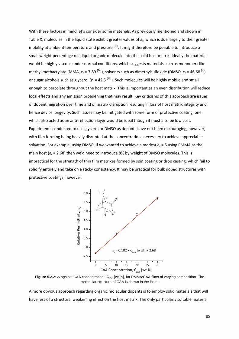
88
With these factors in mind let's consider some materials. As previously mentioned and shown in
Table X, molecules in the liquid state exhibit greater values of εr, which is due largely to their greater
mobility at ambient temperature and pressure [13]. It might therefore be possible to introduce a
small weight percentage of a liquid organic molecule into the solid host matrix. Ideally the material
would be highly viscous under normal conditions, which suggests materials such as monomers like
methyl methacrylate (MMA, εr = 7.89 [14]), solvents such as dimethylsulfoxide (DMSO, εr = 46.68 [4])
or sugar alcohols such as glycerol (εr = 42.5 [15]). Such molecules will be highly mobile and small
enough to percolate throughout the host matrix. This is important as an even distribution will reduce
local effects and any emission broadening that may result. Key criticisms of this approach are issues
of dopant migration over time and of matrix disruption resulting in loss of host matrix integrity and
hence device longevity. Such issues may be mitigated with some form of protective coating, one
which also acted as an anti-reflection layer would be ideal though it must also be low cost.
Experiments conducted to use glycerol or DMSO as dopants have not been encouraging, however,
with film forming being heavily disrupted at the concentrations necessary to achieve appreciable
solvation. For example, using DMSO, if we wanted to achieve a modest εr = 6 using PMMA as the
main host (εr = 2.68) then we'd need to introduce 8% by weight of DMSO molecules. This is
impractical for the strength of thin film matrixes formed by spin coating or drop casting, which fail to
solidify entirely and take on a sticky consistency. It may be practical for bulk doped structures with
protective coatings, however.
Figure 5.2.2: εr against CAA concentration, CCAA [wt %], for PMMA:CAA films of varying composition. The
molecular structure of CAA is shown in the inset.
A more obvious approach regarding organic molecular dopants is to employ solid materials that will
have less of a structural weakening effect on the host matrix. The only particularly suitable material

89
found was camphoric acid anhydride (CAA), which was used by C. F. Madigan and V. Bulović (2003)
to show that solvation is the mechanism causing the observed red-shifts in emission seen in the solid
state previously [11-13, 16]. CAA is a small molecule exhibiting a moderate εr = 12.88 according to
impedance analysis measurements of PMMAx:CAA1-x films of varying composition, as shown in Figure
5.2.2. The impedance analysis method used to determine εr was discussed in chapter 3.3.
The expected linear relationship with increasing CAA concentration is seen with a maximum
permittivity of εr = 5.74 at CCAA = 30 wt%. This sets a practical upper limit for this composite host
system as thin film cohesion breaks down beyond this point. Films including fluorophores at 0.1 wt%
were also measured but no noticeable effect from the fluorophore was seen on εr, which is
unsurprising given their relatively low concentration. Using a composite host of CAA in conjunction
with PMMA provides a platform for assessing the potential of the solvation mechanism and will form
the basis of this investigation, as will be explored in detail in the next section.
The final option for dielectric dopants are inorganic nanoparticles which offer the most technically
challenging but potentially the most promising of solutions. It is necessary to employ very small scale
particles to achieve a well distributed dielectric medium since large particulates are likely to result in
dominant local effects and hence emission broadening. This is in a similar line to the organic
molecular dopants already discussed because of percolation and mobility requirements.
The main reason for the technical challenge this approach faces is the issue of solubility since
inorganic materials do not dissolve in the organic solvents used for solution processing of LSC
materials. It is possible to create a suspension of nanoparticles in a polar solution, ideally water but
also DMSO and alcohols like methanol. However, these solvents are not suitable for processing host
polymers like PMMA, nor are they particularly suited for dissolving the fluorophores. DMSO is an
exception as it is an excellent solvent for almost every material this thesis discusses, however, it has
an extremely high boiling point (189°C) making it almost useless for solution processing at room
temperature. It is worth considering that if processing could be done at higher temperatures of
around 150°C then it may be possible to use DMSO as the solvent for everything. Such techniques
were not available in our laboratories and the extra cost of heat would certainly be detrimental to
overall LSC device cost.
Another way to disperse nanoparticles, although certain to add cost to the device, is to make them
soluble in the desired solvent by use of dispersants or functionalising the particle surface.
Dispersants seem a less hopeful choice for solution processing of solid films as they may add to the
disruptive effect on the matrix. Surface modification therefore seems wisest and can be done for
90
oxide nanoparticles, such as TiO2 (εr ≈ 80 - 100 [6]) or BaSrTiO3 (εr ≈ 1250 [17]) , with phosphonic acids
such as octylphosphonic acid [18] and with silane coupling agents, which themselves allow polymer
grafting to the nanoparticle surface [19]. This last approach, so called fragmentation chain transfer
polymerisation (RAFT), could allow fully functionalised host polymers to be manufactured with high
εr nanoparticles almost woven into the hosts fabric. Another method is to grow the functional
groups in-situ, where surface modification occurs during the nanoparticle synthesis stage via
precursor molecules. This offers benefits, particularly when wanting to disperse the nanoparticles in
low polarity solvents, as for post synthesis modification it is necessary to use a high polarity solvent
to disperse the pure nanoparticles for modification. This is a step that is best avoided due to
concerns of residual aggregates and the need to extract the modified particles, basically by boiling
off the high polarity solvent. Thermal agitation may then disrupt the cohesion of the bonded
functional group, therefore defeating the point. Flushing the high polarity solvent may be successful
by fractionating the suspension using a desired solvent, but it must be both lower density and
immiscible (another two constraints), and then siphoning this layer off the fractionated mixture.
This is in fact precisely the method attempted using ethanol suspensions of 10 nm diameter TiO2
anatase nanoparticles. 10nm nanoparticles were used to enhance dispersion in solution and to
improve the homogeneity of the resultant thin film. Octylphosphonic acid was introduced as a
coupling agent and the suspension was left for over 24hrs to allow the rate of coupling to achieve
high cohesion and then hexane was added to fractionate the mixture. Evaporating the hexane is
then relatively easy (b.p. 68.7°C) and toluene is added to the dried, weighed powder to blend with
PMMA and DCJTB. After a possible false positive increase in Stokes' shift, and problems redispersing
into toluene, it was decided that the approach was somehow flawed and thus this line of inquiry
ended here due to other work. The potential, however, for employing BaSrTiO3 nanoparticles is
obviously impressive, with just 2 wt% of these nanoparticles giving εr = 28 which would make using
CAA as a dielectric additive a pale comparison.. Nanoparticles of this material were acquired but,
with 100 nm diameter, failed to remain in suspension to couple with the phosphonic acid.
5.3 Fluorophore Properties and Choice
Now we'll consider how the properties of the fluorophore itself influences the solvation mechanism.
The energy lost to the reaction field due to the change in dipole moment of the fluorophore upon
excitation is given by Eq. (5.3.1);

91
This can be seen by multiplying Eq. (2.4.2) through by hc which becomes Eq. (5.3.2) in terms of
energy;
Where ΔEstokes is the energy difference between absorption and emission and ΔE0 is the unperturbed
Stokes' shift. Looking at Eq. (5.3.1) if one desires to maximise ΔER then the fluorophore's Onsager
radius, a, must be minimised and the change in dipole moment, Δμ, must be maximised. To explore
the function ER(Δμ, a) a fixed Δf = 0.16 was chosen, which is that for the composite host
PMMA0.7:CAA0.3.
Figure 5.3.1: This 3D colour map shows the energy shift due to solvation as a function of the fluorophore's
physical parameter space for a host of Δf = 0.16.
The 3D colour map exhibited in Fig. 5.3.1 shows a physical parameter space for ΔER(Δμ, a). For large
fluorophores, where a > 10 Å, very little solvation can be achieved owing to the inverse-cubed
proportionality. Additionally the minimum physical size of a fluorescent molecule is limited to
several angstroms which means there is only a small range of a to play with. Larger molecules may
work so long as the fluorescent centre of the molecule is small such as would be expected on
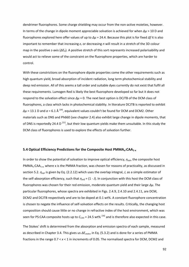
92
dendrimer fluorophores. Some charge shielding may occur from the non-active moieties, however.
In terms of the change in dipole moment appreciable solvation is achieved for when Δμ > 10 D and
fluorophores explored here offer values of up to Δμ = 24.4. Because this plot is for fixed Δf it is also
important to remember that increasing εr or decreasing n will result in a stretch of the 3D colour
map in the positive z-axis (ΔER). A positive stretch of this sort represents increased polarisability and
would act to relieve some of the constraint on the fluorophore properties, which are harder to
control.
With these constrictions on the fluorophore dipole properties come the other requirements such as
high quantum yield, broad absorption of incident radiation, long term photochemical stability and
deep red emission. All of this seems a tall order and suitable dyes currently do not exist that fulfil all
these requirements. Lumogen Red is likely the best fluorophore developed so far but it does not
respond to the solvation effect since Δμ = 0. The next best option is DCJTB of the DCM class of
fluorophores, a class which lacks in photochemical stability. In literature DCJTB is reported to exhibit
Δμ = 13.1 D and a = 6.1 Å [20], equivalent values couldn't be found for DCM and DCM2. Other
materials such as DNS and Ph660 (see chapter 2.4) also exhibit large change in dipole moments, that
of DNS is reportedly 24.4 D [21], but their low quantum yields make them unsuitable. In this study the
DCM class of fluorophores is used to explore the effects of solvation further.
5.4 Optical Efficiency Predictions for the Composite Host PMMAx:CAA1-x
In order to show the potential of solvation to improve optical efficiency, ηopt, the composite host
PMMAx:CAA1-x, where x is the PMMA fraction, was chosen for reasons of practicality, as discussed in
section 5.2. ηopt is given by Eq. (2.2.12) which uses the overlap integral, J, as a simple estimator of
the self-absorption efficiency, such that ηself = (1 - J). In conjunction with this host the DCM class of
fluorophores was chosen for their red emission, moderate quantum yield and their large Δμ. The
particular fluorophores, whose spectra are exhibited in Figs. 2.4.9, 2.4.10 and 2.4.11, are DCM,
DCM2 and DCJTB respectively and are to be doped at 0.1 wt%. A constant fluorophore concentration
is chosen to negate the influence of self-solvation effects on the results. Critically, the changing host
composition should cause little or no change in refractive index of the host environment, which was
seen for PS:CAA composite hosts up to CCAA = 24.5 wt% [16] and is therefore also expected in this case.
The Stokes' shift is determined from the absorption and emission spectra of each sample, measured
as described in Chapter 3.4. This gives us ΔEstokes in Eq. (5.3.2) and is done for a series of PMMA
fractions in the range 0.7 < x < 1 in increments of 0.05. The normalised spectra for DCM, DCM2 and

93
DCJTB are shown in Figures 5.4.1 a), 5.4.1 b) and 5.4.2 a), respectively. These exhibit the change in
emission spectrum as CAA fraction increases. The overlap integral, J, is also measured from the
normalised spectra to be used in conjunction with Eq. (2.2.12) to determine ηopt. From the spectral
plots presented the overlap area is seen to decline as CAA fraction increases.
Figure 5.4.1: The absorption (black) and emission (colour) spectra for a) DCM and b) DCM2 in varying
compositions of the composite host PMMAx:CAA1-x.
Figure 5.4.2: a) The absorption (black) and emission (colour) spectra for DCJTB in varying compositions of the
composite host PMMAx:CAA1-x. b) Various host materials plotted here for εr against n with the zero polarity curve
for reference.
As discussed in chapter 2.4 the Lippert-Mataga equation, Eq. (2.4.2), allows us to predict the shift in
energy due to the solvation effect. To use this predictive power several quantities must first be
determined. First is to determine the unperturbed Stokes' shift, ΔE0. To do this a host of zero
polarisability, Δf = 0, is needed and then the fluorophore emission and absorption spectra are
measured in this host. The difference between the peak energies of these gives ΔE0. By plotting
various host material’s optical parameters against the zero polarity line given by εr = n2, as shown in
Figure 5.4.2 b), it is simple to choose a material for this task. Paraffin wax, or parawax, is an obvious
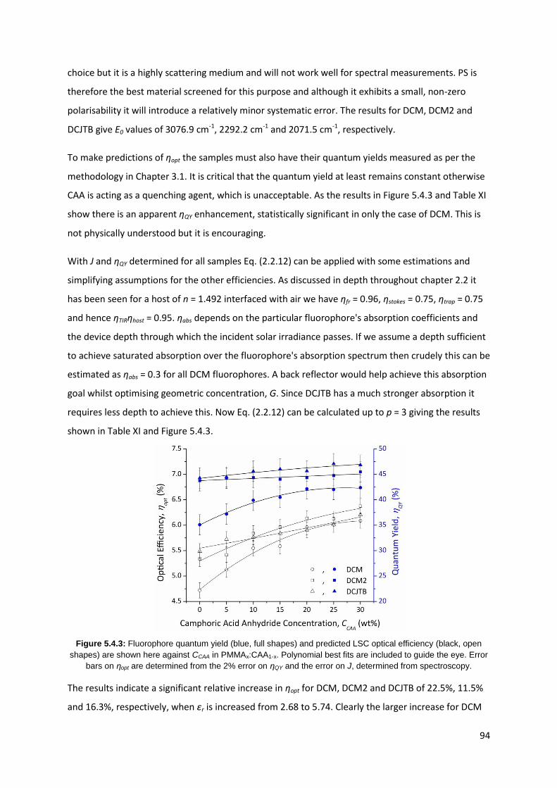
94
choice but it is a highly scattering medium and will not work well for spectral measurements. PS is
therefore the best material screened for this purpose and although it exhibits a small, non-zero
polarisability it will introduce a relatively minor systematic error. The results for DCM, DCM2 and
DCJTB give E0 values of 3076.9 cm-1, 2292.2 cm-1 and 2071.5 cm-1, respectively.
To make predictions of ηopt the samples must also have their quantum yields measured as per the
methodology in Chapter 3.1. It is critical that the quantum yield at least remains constant otherwise
CAA is acting as a quenching agent, which is unacceptable. As the results in Figure 5.4.3 and Table XI
show there is an apparent ηQY enhancement, statistically significant in only the case of DCM. This is
not physically understood but it is encouraging.
With J and ηQY determined for all samples Eq. (2.2.12) can be applied with some estimations and
simplifying assumptions for the other efficiencies. As discussed in depth throughout chapter 2.2 it
has been seen for a host of n = 1.492 interfaced with air we have ηfr = 0.96, ηstokes = 0.75, ηtrap = 0.75
and hence ηTIRηhost = 0.95. ηabs depends on the particular fluorophore's absorption coefficients and
the device depth through which the incident solar irradiance passes. If we assume a depth sufficient
to achieve saturated absorption over the fluorophore's absorption spectrum then crudely this can be
estimated as ηabs = 0.3 for all DCM fluorophores. A back reflector would help achieve this absorption
goal whilst optimising geometric concentration, G. Since DCJTB has a much stronger absorption it
requires less depth to achieve this. Now Eq. (2.2.12) can be calculated up to p = 3 giving the results
shown in Table XI and Figure 5.4.3.
Figure 5.4.3: Fluorophore quantum yield (blue, full shapes) and predicted LSC optical efficiency (black, open
shapes) are shown here against CCAA in PMMAx:CAA1-x. Polynomial best fits are included to guide the eye. Error
bars on ηopt are determined from the 2% error on ηQY and the error on J, determined from spectroscopy.
The results indicate a significant relative increase in ηopt for DCM, DCM2 and DCJTB of 22.5%, 11.5%
and 16.3%, respectively, when εr is increased from 2.68 to 5.74. Clearly the larger increase for DCM
95
is a result of the larger apparent increase in ηQY for that fluorophore since the decrease in J is
proportionately similar in all cases. The resultant optical efficiency is almost the same across the
DCM class exhibited here which is anticipated when looking at the relative sizes of ηQY and J. DCM
achieves a smaller overlap integral but exhibits lower quantum yield and vice versa is true for both
DCM2 and DCJTB. Tentatively DCJTB shows itself to be the best fluorophore in this set.
Using the data from the PMMAx:CAA1-x composite host system it is possible to make predictions of
the limits of solvation in the context of improving LSC efficiency. To do this a Lippert plot is
produced, which is a plot of Δν against Δf as shown in Figure 5.4.4, along with a linear best fit
interpolated to high Δf. Out of curiosity for exploring higher permittivity parameter space the host
PVDF-HFP (see Table X) is used pure with DCM, DCM2 and DCJTB as dopants. PVDF-HFP has εr =
11.38 and n = 1.407 (hence Δf = 0.2393), which represents a significant advance on the composite
PMMA0.7:CAA0.3 having εr = 5.74 with n = 1.492 (hence Δf = 0.155).
Figure 5.4.4: Lippert plot for DCM, DCM2 and DCJTB with linear best fits interpolated to Δf = 0.2505, which is
the equivalent of εr = 30 with n = 1.492. For each dye the leftmost data point is for a pure PS host where Δf = 0
and the rightmost data point is for pure PVDF-HFP where Δf = 0.2393.
Figure 5.4.4 shows the linear trend predicted by the Lippert-Mataga equation, Eq. (2.4.2), and serves
as an indication that solvation is indeed the mechanism responsible for the observed energy shifts.,
One notices that, amongst the seven PMMAx:CAA1-x data points for each fluorophore, despite their
being evenly spaced in terms of PMMA fraction, the x-axis interval between data points is not
constant. This is because of the dependence of Δf on εr, as plotted in Fig. 5.2.1, resulting in a
diminishing return on Δν for higher εr. From the line equations of the linear best fits in Fig. 5.4.4 we
then find Δν for Δf = 0.2505 (εr = 30 with n = 1.492) to be 4624 cm-1, 4156 cm-1 and 3904 cm-1 for
DCM, DCM2 and DCJTB, respectively. This is shown in Table XI, along with calculated values of ηopt,

96
which represent an improvement relative to pure PMMA of 24.5%, 18.6% and 23.4% for DCM, DCM2
and DCJTB, respectively. Values for PVDF-HFP are also shown with assumed quantum yields in line
with that measured for the fluorophores in PMMA. Looking back to Table IV on page 43 DCM shows
a higher quantum yield in PVDF-HFP than PMMA but the yield was not measured for the other
fluorophores and so this data was not employed here.
Dye CCAA [wt%] εr J [%] νPL [cm-1] νabs [cm-1] Δν [cm-1] ηQY [±0.02] ηopt [%]
DCM
0 2.68 16.2 18248 21459 3211 0.35 4.72
5 3.19 13.1 17889 21459 3570 0.37 5.12
10 3.70 13.0 17889 21459 3570 0.40 5.55
15 4.23 12.1 17857 21459 3602 0.40 5.59
20 4.73 11.0 17637 21459 3823 0.42 5.96
25 5.26 10.0 17544 21459 3915 0.42 6.01
30 5.74 9.3 17452 21459 4007 0.42 6.09
(PVDF-HFP) 11.38 6.0 17123 21459 4336 0.42 6.19
Theoretical 30 4.7 16921 21459 4624 0.42 6.25
DCM2
0 2.68 24.7 17253 19960 2707 0.44 5.49
5 3.19 20.3 17011 19960 2949 0.44 5.73
10 3.70 19.6 16863 19960 3097 0.44 5.77
15 4.23 18.2 16776 19960 3184 0.44 5.84
20 4.73 16.9 16646 19960 3314 0.44 5.91
25 5.26 14.9 16604 19960 3356 0.44 6.01
30 5.74 13.3 16491 19960 3469 0.45 6.21
(PVDF-HFP) 11.38 6.3 16051 19960 3909 0.45 6.55
Theoretical 30 3.8 15804 19960 4156 0.45 6.74
DCJTB
0 2.68 28.0 17361 19802 2441 0.44 5.34
5 3.19 26.7 17212 19802 2590 0.44 5.42
10 3.70 24.0 17065 19802 2737 0.46 5.84
15 4.23 21.8 16863 19802 2939 0.46 5.96
20 4.73 18.6 16722 19802 3080 0.46 6.14
25 5.24 18.8 16639 19802 3163 0.46 6.12
30 5.74 16.8 16529 19802 3273 0.47 6.38
(PVDF-HFP) 11.38 7.7 16041 19802 3761 0.47 6.85
Theoretical 30 5.3 15873 19802 3904 0.47 6.97
Table XI: Solvation study results for the composite host PMMAx:CAA1-x with DCM type fluorophore's doped at 0.1
wt%. Also included are values for pure PVDF-HFP and predicted values for εr = 30.
DCJTB is still the favourite achieving an optical efficiency of 7% or 0.07. Combined with an LSC having
a reasonable geometric ratio of G = 30 this would give a total optical concentration of Copt = 0.07 x 30
= 2.1. Then solar cells collecting along the edge of such an LSC device would be receiving around
twice the irradiant intensity of the incident solar intensity. Higher geometric ratios could be possible
but, as discussed in chapter 2.5, current best LSC devices are quite small and exhibit geometric ratios
of around G = 2.5 giving, in the case of DCJTB here, Copt = 0.07x2.5 = 0.175. Clearly this is poor and
97
would be making a waste of solar cells. We thus learn that the geometry of the device is critical and
must remind ourselves that there are losses associated with increasing G due to the mean path
length increasing, such as self-absorption quantified by ηself.
Another point of interest is to make a fit of the data to Eq. (2.4.2) as a function of εr. Partially to this
end the unperturbed Stokes' shift, ΔE0, was determined using PS as a host for Δf = 0. Models of Eq.
(2.4.2) are to be produced for variable εr and n = 1.492 and so in addition the fluorophore properties,
Δμ and a, must be determined.
First the Onsager Radius, a, is calculated theoretically through quantum chemical calculations, using
the GAMESS software [22], of energetically optimised ground state geometries using a combination of
B3LYP [23] functional and 6-31G* [24] basis sets. These were found to be 5.20 Å, 5.49 Å and 6.18 Å for
DCM, DCM2 and DCJTB, respectively. This work was carried out by Keith T. Butler.
Next the change in dipole moment, Δμ, is determined from the gradient of the best fit lines of Figure
5.4.4. Recalling Eq. (2.4.2) and comparing it to a straight line, for y = Δν and x = Δf, the change in
dipole moment can be shown to be given by Eq. (5.4.1);
Where m is the gradient and, in cgs units, h is Planck's constant (6.626x10⁻²⁷ erg s) and c is the speed
of light (2.9979x1010 cm s-1). The Onsager radius was found as described above and so applying Eq.
(5.4.1) for DCM, DCM2 and DCJTB the change in dipole was found to be 12.1 ± 0.8 D, 10.2 ± 0.2 D
and 13.0 ± 0.4 D, respectively. The errors are determined from the standard error on the gradient of
the lines of best fit in Fig. 5.4.4. What has been done here is to use quantum chemical models in
conjunction with measured energy shift data to indirectly determine Δμ through the assumption of
Eq. (2.4.2)'s validity. The value for DCJTB found here is consistent with the value of 13.1 D found in
literature [20].
Using the determined values of Δμ and a with fixed n = 1.492, Eq. (2.4.2) can now be employed to
model the variation in ΔE as a function of εr as shown in Figure 5.4.5. This time ΔE is used in place of
Δν for clarity; the LM equation can be rewritten in terms of energy by multiplying through by hc.
Fig. 5.4.5 shows how the data for doped PMMAx:CAA1-x hosts nicely follows the theoretical line of
Lippert-Mataga theory. Notice that the PS sample data points drop low relative to the trend, which is
owing to the higher refractive index of PS. Similar is true of PVDF-HFP, whose index is lower (refer

98
back to Fig. 5.2.1 to see how n influences Δf and hence Δν). Thus the models of Figure 5.4.5 only
truly apply to the PMMAx:CAA1-x composite host system.
Figure 5.4.5: This plot of ΔE against εr shows the data for DCM, DCM2 and DCJTB plotted with models of Eq.
(2.4.2) tuned by the value of Δμ. As before PS samples are leftmost, the rightmost data points are for pure PVDF-
HFP and the rest in the middle are for various compositions of PMMAx:CAA1-x.
Figure 5.4.5 has similarities in form to Figure 5.2.1 as a result of the εr dependence, although other
influences are present in the former (namely n, Δμ and a). They both give insight into the upper
limits achievable through solvation indicating a plateau in Δν at around εr = 30 to 40. This would
remain the case whatever values the other key parameters take.
5.5 Conclusions
In this study it has been show that, for the DCM class fluorophores exhibited here, a potential
relative increase in optical efficiency of between 18.6% and 24.5% is possible. These theoretical
limits are for a relative permittivity of εr = 30 and are nearly reached using PVDF-HFP as a host
material. The limit at εr = 30 is predicted by varying the mass fractions of the composite host
PMMAx:CAAx-1 doped with a given fluorophore at 0.1 wt%. The fluorescence quantum yield was seen
to remain steady as CAA fraction increases, which indicates CAA does not act as a quenching agent.
This is a crucial condition to make gains from the solvation effect for luminescent solar concentrator
devices.
A maximum LSC optical efficiency of ηopt = 0.07 was seen for DCJTB with reasonable assumptions for
other efficiencies. With developments in fluorophore design to improve properties such as quantum

99
yield, spectral absorption and photochemical stability, the solvation mechanism could prove a useful
enhancement tool to achieve higher optical concentrations in LSC devices, therefore to extract more
energy. The technique also requires availability of low cost dielectric dopants to enhance host
permittivity, or similarly low cost high permittivity host materials.

100
5.6 References
[1] A. P. Green, K. T. Butler and A. R. Buckley, Tuning of the emission energy of fluorophores using
solid state solvation for efficient luminescent solar concentrators, App. Phys. Lett. 102, 133501
(2013)
[2] R. Bose, D. J. Farrell, A. J. Chatten, M. Pravettoni, A. Büchtemann and K. W. J. Barnham, Novel
Configurations of Luminescent Solar Concentrators, Proc. 22nd European Photovoltaic Solar Energy
Conference, pp. 210-214, (2007)
[3] R. Bose, D. J. Farrell, A. J. Chatten, M. Pravettoni, A. Büchtemann, J. Quilitz, A. Fiore, L. Manna
and K. W. J. Barnham, Luminescent Solar Concentrators: Nanorods and Raytrace Modelling, 33rd.
IEEE Photovoltaic Specialists Conference, pp. 1- 5, (2008)
[4] Louisiana State University, http://macro.lsu.edu/HowTo/solvents.htm
[5] Kok Chemware, (1999-2002)
http://www.sanderkok.com/techniques/hplc/eluotropic_series_extended.html
[6] The Goodfellow Group, (2008 - 2013) http://www.goodfellow.com/
[7] Mikhail Polyanskiy, Refractive Index Info, (2008 - 2013) http://refractiveindex.info/
[8] K. Shinyama, T. Oi and S. Fujita, Dielectric Relaxation Phenomenon of Polylactic Acid with β-
Crystalline Chitin, Int. J. Polym. Sci. 2012, 389491 (2012)
[9] D. Garlotta, A Literature Review of Poly(Lactic Acid), J. Polym. Environ. 9, 2, 63 - 84 (2001)
[10] Sigma Aldrich, Poly(vinylidene fluoride-co-hexafluoropropylene) (PVDF-HFP)
http://www.sigmaaldrich.com/catalog/product/aldrich/427187?lang=en®ion=GB
[11] V. Bulović, A. Shoustikov, M. A. Baldo, E. Bose, V. G. Kozlov, M. E. Thompson and S. R. Forrest,
Bright, saturated, re-to-yellow organic light-emitting devices based on polarization-induced spectral
shifts, Chem. Phys. Lett. 287, 455 - 460 (1998)
[12] V. Bulović, R. Deshpande, M. E. Thompson and S. R. Forrest, Tuning the color emission of thin
film molecular oraganic light emitting devices by the solid state solvation effect, Chem. Phys. Lett.
308, 317 - 322 (1999)
[13] R. E. Sau and G. Baur, Influence of the Solvent Matrix on the Overlapping of the Absorption and
Emission Bands of Solute Fluorescent Dyes, Appl. Phys. 23, 369 - 372 (1980)
101
[14] F. Liakath Ali Khan, P. Sivagurunathan, S. Raja Mohamed Kamil and S. C. Mehrotra, Dielectric
studies of methyl methacrylate and butyl methacrylate with primary alcohols using time domain
reflectometry, Indian J. Pure Appl. Phys. 45, 754 - 758 (2007)
[15] Clipper Controls Inc., http://www.clippercontrols.com/pages/Dielectric-Constant-
Values.html#M, (2013)
[16] C. F. Madigan and V. Bulović, Solid State Solvation in Amorphous Organic Thin Films, Phys. Rev.
Lett. 91, 24, 247403 (2003)
[17] R. Balachandran, B. H. Ong, H. Y. Wong, K. B. Tan and M. Muhamad Rasat, Dielectric
Characteristics of Barium Strontium Titanate Based Metal Insulator Metal Capacitor for Dynamic
Random Access Memory Cell, Int. J. Electrochem. Sci. 7, 11895 - 11903 (2012)
[18] A. Colombo, F. Tassone, F. Santolini, N. Contiello, A. Gambirasio and R. Simonutti, Nanoparticle-
doped large area PMMA plates with controlled optical diffusion, J. Mater. Chem. C 1, 2927 - 2934
(2013)
[19] M. Iijima and H. Kamiya, Surface Modification for Improving the Stability of Nanoparticles in
Liquid Media, Powd. Part. J. 27, 119 - 129 (2009)
[20] Y. Yao, Q. Zhou, X. Wang, Y. Wang and B. Zhang, A DCM-Type Red-Fluorescent Dopant for High-
Performance Organic Electroluminescent Devices, Adv. Funct. Mater. 17, 93 - 100 (2007)
[21] J. M. Warman, M. P. De Haas and A. Hummel, Dipole Moment Changes in the Singlet and Triplet
Excited States of 4-Dimethylamino-4’-nitrostilbene Detected by Nanosecond Time-Resolved
Microwave Conductivity, Chem. Phys. Lett. 87, 1 (1982)
[22] M. W. Schmidt, K. K. Baldridge, J. A. Boatz, S. T. Elbert, M. S. Gordon, J. H. Hansen, S. Koseki, N.
Matsunuga, K. A. Nguyen, S. Su, T. L. Windus, M. Dupuis and J. A. Montgomery Jr., General atomic
and molecular electronic structure system, J. Comput. Chem. 14, 1347 - 1363 (1993)
[23] A. D. Becke, Density-functional thermochemistry. III. The role of exact exchange, J. Chem. Phys.
98, 5648 - 5652 (1993)
[24] M. M. Francl, W. J. Pietro, W. J. Hehre, J. S. Binkley, M. S. Gordon, D. J. Defrees and J. A. Pople,
Self-consistent molecular orbital methods. XXIII. A polarisation-type basis set for second-row
elements, J. Chem. Phys. 77, 3654 - 3665 (1982)
102
Chapter 6
Parameter Screening for Spray Coating Deposition of Surface
Coated Luminescent Solar Concentrators
6.1 Introduction
This chapter is an examination of the results of a screening study to explore the influence of
different operational parameters of a spray coating deposition system. Spray coating offers a fast,
low cost and large area deposition methodology for surface coating LSC devices with a fluorophore
containing layer. To better understand the spray coating method a parameter screening study has
been used. Screening approaches offer a fast and statistically powerful method to assess how the
operational parameters affect the film qualities that are of interest.
Spray coating is relatively complex when compared to other deposition methods because of the
large number of operational parameters, or factors, involved. In the terminology of screening
experiments factors are independent variables which may affect the outcome of the experiment. For
example all deposition methods rely in some manner on the solvent and on the solute
concentrations, and so also the viscosity of the solution. Similarly they can also all utilise film forming
control techniques, such as control of vapour pressure and fume extraction rate, and substrate
conditioning such as plasma ashing or surface modification. These all affect the resultant film
deposited but apart from these universal factors each deposition method carries personalised
factors.
Spin coater operation relies on spin speed and is ill suited to large area deposition. Spin coating finds
use in small area research applications and not in production scale methods. Also ill suited to large
area deposition is dip coating which depends on withdrawal speed from the coating trough. Dip
coating could be suitable for small LSC devices on the scale of 10 cm or so but would lack high
production speeds offered by spray coating. Bar coating, which could be a potential method for high
speed, large area depositions, depends on the number of winds of wire per unit length, the wire
thickness and the carrying speed (the speed the bar travels at). Doctor blading is similar in many
respects to bar coating and is well suited to large area deposition. It depends on the distance
between the blade and substrate and the carrying speed. For spray coating deposition the
Chapter 6: Parameter Screening for Spray Coating Deposition of Surface Coated LSCs
103
dependences include injection pressure, spray head speed and height, substrate temperature and
the number of coatings. It is because of this number of factors that a screening study was preferred.
The film quality in this study is assessed by 7 measured dependent variables, or responses, which are
the roughness ratio, <RR>, the standard deviation of this, σR, the height range, Rh, the average film
thickness, <t>, the relative absorption intensity, Iabs, the change in Stokes' shift, ΔλPL and a de-
broadening parameter. The screening experiment is designed and built using JMP statistical software
developed by SAS Institute Inc. JMP uses a random seed to build an experiment consisting of a
number of samples with associated factor values for their fabrication. The program ensures by the
arrangement of factor values that the parameter space is explored thoroughly in as few samples as
possible.
As discussed through Chapter 2.3 an ideal geometry to apply such coatings to would be that of a
multi-cylindrical structure [1], though here only square planar type structures are explored. Multi-
cylindrical PC substrates were produced for this study by injection moulding but were found to be
unsuitable due to the solvents being used for the coating. Instead standard microscope slides of 75
mm x 25 mm x 1 mm (hence G = 9.375) are employed and are made of soda-lime glass having
refractive index n3 = 1.52. It is important for the undoped core of the surface doped LSC to have a
higher refractive index than the doped coating, which is in this case PMMA with n2 = 1.492 and this is
interfaced with air having n1 = 1. This is a requirement due to the laws of refraction as fluoresced
light in the active coating will not be waveguided through the core if n2 > n3 [2]. Instead in such a
device light would be trapped in the active coating which is by design a highly absorbing medium
and hence strong attenuation is expected. Optimisation by reduction of mean path length travelled
through the LSC is achieved for minimisation of the ratio n2/n3. This must be optimised in tandem
with n1/n2 due to Fresnel reflection (Eqs. (2.2.2) and (2.2.3)) and trapping efficiency (Eq. (2.2.4)) and,
as seen in the last chapter, if solvation is employed the orientational polarisability must also be
optimised through n2, as described by Eq. (5.2.1).
6.2 Spray Coating Parameter Space
What follows now is a detailed look at the spray-coating deposition method, starting with specific
consideration of the functional parameters, or factors. This discussion will follow on to develop the
output metrics, or responses, which shall be used to ascertain the effectiveness of a given set of
input factors at depositing active coatings onto soda-lime glass microscope slides. Chapter 3.4
provides a diagram and technical details of the Prism Ultra-Coat 300 spray-coating system and its

Chapter 6: Parameter Screening for Spray Coating Deposition of Surface Coated LSCs
104
operation. Fig. 6.2.1 shows a schematic of a spray deposition to help illustrate the parameters in the
process.
Figure 6.2.1: Schematic infographic of a spray deposition showing the factors chosen for optimisation and the
materials employed. The spray head moves with speed s, at height h with injection pressure, Pin. The LSC
concentration formulation consists of a host:dye blend with total concentration, Ctot, and dye concentration, Cdye,
in some solvent and is deposited onto a glass microscope slide at temperature, T. The number of coats, Ncoat, is
also considered.
In spray coating there are many variables that need mutual optimisation, from those of the material
blend to be sprayed to those of the spray system itself. These include the dye and host materials,
their concentrations, choice of solvent, spray head height, speed and injection pressure, to name
just a few. Clearly taking either a trial and error or a full factorial approach over such a range of
parameters, many of which are continuous in nature and thus occupy a very large space, is
nonsensical. Trial and error approaches look at detailed cross sections through the parameter space
by picking one factor and varying it continuously to find the optimum, and then moving on to the
next factor. This never captures the full response surface, unlike the full factorial study which
explores the whole parameter space but is very costly in materials and time. By contrast the
screening study design saves time and materials by exploring the entire response surface with as few
samples as necessary. Screening experiments employ the idea of the sparsity principle (sparsity-of-
effects principle), which advises a screening approach to the problem of having many known factors
of which most will be essentially inactive and/or trivial in the responses that are of interest. The
sparsity-of-effects principle assumes that the process under consideration is dominated by only a
few key effects of statistical significance [3,4].
Here the sparsity principle is applied to the spray coating technique in the form of an effect
screening experiment. Nine key factors were chosen for mutual optimisation, discussed in the next

Chapter 6: Parameter Screening for Spray Coating Deposition of Surface Coated LSCs
105
paragraphs, and these are either continuous or discrete in nature. The factors are illustrated in Fig.
6.2.1 and the parameter settings are tabulated in Table XII by sample. Those parameters that are
continuous are designated physically reasonable maximum and minimum values for which the
deposition system can operate. Discrete factors are designated 2 or 3 discrete values.
First is the total concentration of the polymer:dye blend, Ctot, which is the sum of the host polymer
(PMMA) and dye concentrations in units of g/l. Some experimentation was necessary to appreciate
the tolerances of the spray coating system in this regard; if Ctot is set too high then we find higher
pressures are required and eventually the material loading is too great and one observes polymer
threads forming mid-air in streamers like candyfloss. A maximum workable concentration for PMMA
loading was found to be roughly at Ctot = 120 g/l and a minimum was set at Ctot = 50 g/l.
The dye concentration, Cdye, in wt% units was also chosen to see if this affects the film forming
properties and because it is expected to have strong importance on absorption processes. Minimum
and maximum were taken to be 0.3% and 1% respectively. This range is chosen by appreciation of
dye extinction and concentration quenching of quantum yield; a certain concentration is required to
absorb incoming light but too high a concentration will result in lower rates of radiative
recombination. The arguments for these values are explored in more detail shortly when considering
goal setting for the thickness response, <t>.
The dye type is chosen to understand the influence of particular dye properties. This is set to be a
two-level categorical factor with the non-polar dye PR and the polar dye DCJTB favoured for this
study. DCJTB exhibits stronger intrinsic absorption than PR but has lower quantum yield at any given
concentration.
Next the solvent used is designated a 3-level categorical with polar solvents chlorobenzene (CB),
anisole (AS) and non-polar toluene (T) chosen for study. Toluene has a lower boiling point (110.6°C)
than CB (131.7°C) or AS (155.5°C) and so films from this solvent will dry faster, which may have
strong influence on the resultant film particularly with regards to surface roughness.
Injection pressure, Pin, is an important continuous factor characterising the rate of flow of material
onto the ultrasonic tip of the spray head. Higher pressures should result in greater thicknesses but
there is a need to explore what other effects pressure may have, particularly regarding film surface
effects. Some experimentation was needed to properly ascertain workable pressure ranges with the
concentrations of solution used. If the pressure is too low at a given concentration then little
material is injected and a proper spray is not formed. Too high a pressure and the spray becomes a
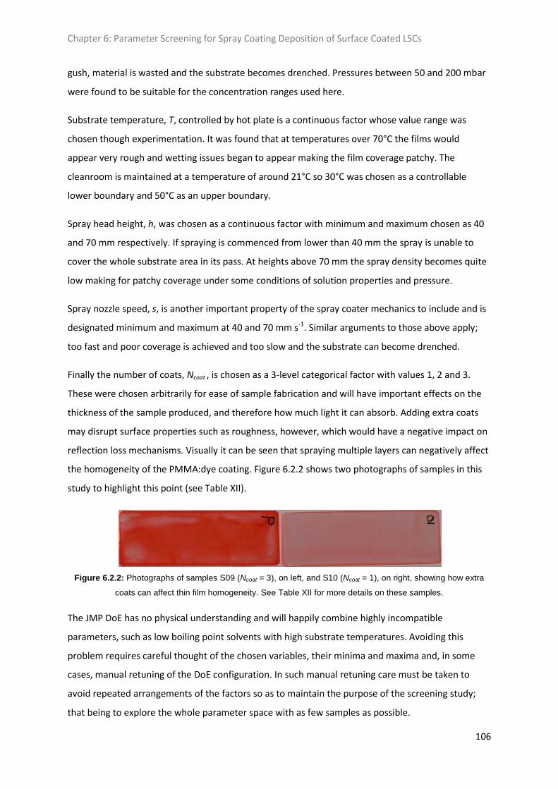
Chapter 6: Parameter Screening for Spray Coating Deposition of Surface Coated LSCs
106
gush, material is wasted and the substrate becomes drenched. Pressures between 50 and 200 mbar
were found to be suitable for the concentration ranges used here.
Substrate temperature, T, controlled by hot plate is a continuous factor whose value range was
chosen though experimentation. It was found that at temperatures over 70°C the films would
appear very rough and wetting issues began to appear making the film coverage patchy. The
cleanroom is maintained at a temperature of around 21°C so 30°C was chosen as a controllable
lower boundary and 50°C as an upper boundary.
Spray head height, h, was chosen as a continuous factor with minimum and maximum chosen as 40
and 70 mm respectively. If spraying is commenced from lower than 40 mm the spray is unable to
cover the whole substrate area in its pass. At heights above 70 mm the spray density becomes quite
low making for patchy coverage under some conditions of solution properties and pressure.
Spray nozzle speed, s, is another important property of the spray coater mechanics to include and is
designated minimum and maximum at 40 and 70 mm s-1. Similar arguments to those above apply;
too fast and poor coverage is achieved and too slow and the substrate can become drenched.
Finally the number of coats, Ncoat , is chosen as a 3-level categorical factor with values 1, 2 and 3.
These were chosen arbitrarily for ease of sample fabrication and will have important effects on the
thickness of the sample produced, and therefore how much light it can absorb. Adding extra coats
may disrupt surface properties such as roughness, however, which would have a negative impact on
reflection loss mechanisms. Visually it can be seen that spraying multiple layers can negatively affect
the homogeneity of the PMMA:dye coating. Figure 6.2.2 shows two photographs of samples in this
study to highlight this point (see Table XII).
Figure 6.2.2: Photographs of samples S09 (Ncoat = 3), on left, and S10 (Ncoat = 1), on right, showing how extra
coats can affect thin film homogeneity. See Table XII for more details on these samples.
The JMP DoE has no physical understanding and will happily combine highly incompatible
parameters, such as low boiling point solvents with high substrate temperatures. Avoiding this
problem requires careful thought of the chosen variables, their minima and maxima and, in some
cases, manual retuning of the DoE configuration. In such manual retuning care must be taken to
avoid repeated arrangements of the factors so as to maintain the purpose of the screening study;
that being to explore the whole parameter space with as few samples as possible.
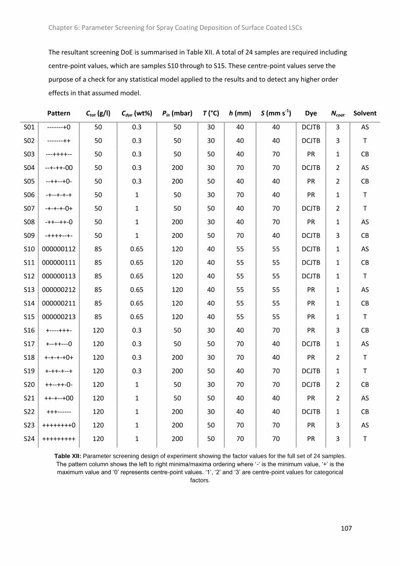
Chapter 6: Parameter Screening for Spray Coating Deposition of Surface Coated LSCs
107
The resultant screening DoE is summarised in Table XII. A total of 24 samples are required including
centre-point values, which are samples S10 through to S15. These centre-point values serve the
purpose of a check for any statistical model applied to the results and to detect any higher order
effects in that assumed model.
Pattern Ctot (g/l) Cdye (wt%) Pin (mbar) T (°C) h (mm) S (mm s-1) Dye Ncoat Solvent
S01 -------+0 50 0.3 50 30 40 40 DCJTB 3 AS
S02 -------++ 50 0.3 50 30 40 40 DCJTB 3 T
S03 ---++++-- 50 0.3 50 50 40 70 PR 1 CB
S04 --+-++-00 50 0.3 200 30 70 70 DCJTB 2 AS
S05 --++--+0- 50 0.3 200 50 40 40 PR 2 CB
S06 -+--+-+-+ 50 1 50 30 70 40 PR 1 T
S07 -+-+-+-0+ 50 1 50 50 40 70 DCJTB 2 T
S08 -++--++-0 50 1 200 30 40 70 PR 1 AS
S09 -++++--+- 50 1 200 50 70 40 DCJTB 3 CB
S10 000000112 85 0.65 120 40 55 55 DCJTB 1 AS
S11 000000111 85 0.65 120 40 55 55 DCJTB 1 CB
S12 000000113 85 0.65 120 40 55 55 DCJTB 1 T
S13 000000212 85 0.65 120 40 55 55 PR 1 AS
S14 000000211 85 0.65 120 40 55 55 PR 1 CB
S15 000000213 85 0.65 120 40 55 55 PR 1 T
S16 +----+++- 120 0.3 50 30 40 70 PR 3 CB
S17 +--++---0 120 0.3 50 50 70 40 DCJTB 1 AS
S18 +-+-+-+0+ 120 0.3 200 30 70 40 PR 2 T
S19 +-++-+--+ 120 0.3 200 50 40 70 DCJTB 1 T
S20 ++--++-0- 120 1 50 30 70 70 DCJTB 2 CB
S21 ++-+--+00 120 1 50 50 40 40 PR 2 AS
S22 +++------ 120 1 200 30 40 40 DCJTB 1 CB
S23 ++++++++0 120 1 200 50 70 70 PR 3 AS
S24 +++++++++ 120 1 200 50 70 70 PR 3 T
Table XII: Parameter screening design of experiment showing the factor values for the full set of 24 samples.
The pattern column shows the left to right minima/maxima ordering where ‘-‘ is the minimum value, ‘+’ is the
maximum value and ‘0’ represents centre-point values. ‘1’, ‘2’ and ‘3’ are centre-point values for categorical
factors.
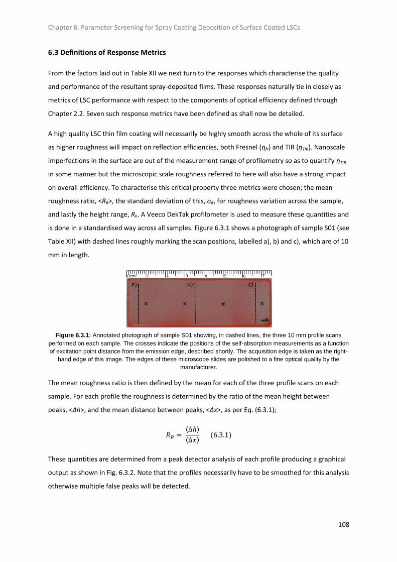
Chapter 6: Parameter Screening for Spray Coating Deposition of Surface Coated LSCs
108
6.3 Definitions of Response Metrics
From the factors laid out in Table XII we next turn to the responses which characterise the quality
and performance of the resultant spray-deposited films. These responses naturally tie in closely as
metrics of LSC performance with respect to the components of optical efficiency defined through
Chapter 2.2. Seven such response metrics have been defined as shall now be detailed.
A high quality LSC thin film coating will necessarily be highly smooth across the whole of its surface
as higher roughness will impact on reflection efficiencies, both Fresnel (ηfr) and TIR (ηTIR). Nanoscale
imperfections in the surface are out of the measurement range of profilometry so as to quantify ηTIR
in some manner but the microscopic scale roughness referred to here will also have a strong impact
on overall efficiency. To characterise this critical property three metrics were chosen; the mean
roughness ratio, <RR>, the standard deviation of this, σR, for roughness variation across the sample,
and lastly the height range, Rh. A Veeco DekTak profilometer is used to measure these quantities and
is done in a standardised way across all samples. Figure 6.3.1 shows a photograph of sample S01 (see
Table XII) with dashed lines roughly marking the scan positions, labelled a), b) and c), which are of 10
mm in length.
Figure 6.3.1: Annotated photograph of sample S01 showing, in dashed lines, the three 10 mm profile scans
performed on each sample. The crosses indicate the positions of the self-absorption measurements as a function
of excitation point distance from the emission edge, described shortly. The acquisition edge is taken as the right-
hand edge of this image. The edges of these microscope slides are polished to a fine optical quality by the
manufacturer.
The mean roughness ratio is then defined by the mean for each of the three profile scans on each
sample. For each profile the roughness is determined by the ratio of the mean height between
peaks, <Δh>, and the mean distance between peaks, <Δx>, as per Eq. (6.3.1);
These quantities are determined from a peak detector analysis of each profile producing a graphical
output as shown in Fig. 6.3.2. Note that the profiles necessarily have to be smoothed for this analysis
otherwise multiple false peaks will be detected.
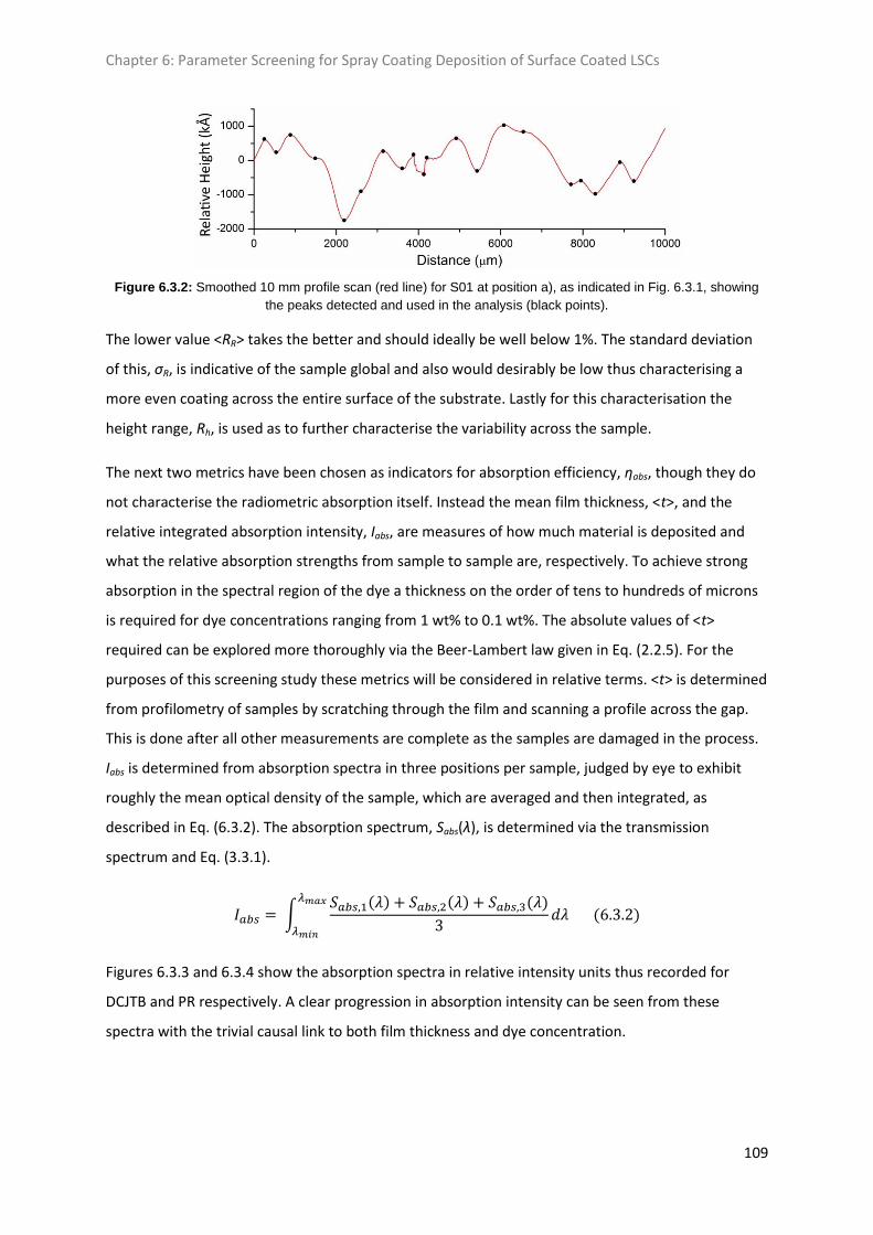
Chapter 6: Parameter Screening for Spray Coating Deposition of Surface Coated LSCs
109
Figure 6.3.2: Smoothed 10 mm profile scan (red line) for S01 at position a), as indicated in Fig. 6.3.1, showing
the peaks detected and used in the analysis (black points).
The lower value <RR> takes the better and should ideally be well below 1%. The standard deviation
of this, σR, is indicative of the sample global and also would desirably be low thus characterising a
more even coating across the entire surface of the substrate. Lastly for this characterisation the
height range, Rh, is used as to further characterise the variability across the sample.
The next two metrics have been chosen as indicators for absorption efficiency, ηabs, though they do
not characterise the radiometric absorption itself. Instead the mean film thickness, <t>, and the
relative integrated absorption intensity, Iabs, are measures of how much material is deposited and
what the relative absorption strengths from sample to sample are, respectively. To achieve strong
absorption in the spectral region of the dye a thickness on the order of tens to hundreds of microns
is required for dye concentrations ranging from 1 wt% to 0.1 wt%. The absolute values of <t>
required can be explored more thoroughly via the Beer-Lambert law given in Eq. (2.2.5). For the
purposes of this screening study these metrics will be considered in relative terms. <t> is determined
from profilometry of samples by scratching through the film and scanning a profile across the gap.
This is done after all other measurements are complete as the samples are damaged in the process.
Iabs is determined from absorption spectra in three positions per sample, judged by eye to exhibit
roughly the mean optical density of the sample, which are averaged and then integrated, as
described in Eq. (6.3.2). The absorption spectrum, Sabs(λ), is determined via the transmission
spectrum and Eq. (3.3.1).
Figures 6.3.3 and 6.3.4 show the absorption spectra in relative intensity units thus recorded for
DCJTB and PR respectively. A clear progression in absorption intensity can be seen from these
spectra with the trivial causal link to both film thickness and dye concentration.

Chapter 6: Parameter Screening for Spray Coating Deposition of Surface Coated LSCs
110
Figure 6.3.3: Averaged relative intensity absorption spectra for DCJTB samples.
Figure 6.3.4: Averaged relative intensity absorption spectra for PR samples.
The final two metrics are the change in Stokes' shift, ΔλPL, and the de-broadening parameter, Δw,
relate directly to the self-absorption loss mechanism, quantified by the efficiency ηself, and use a
spectroscopy method specific to this chapter. This method shown in Fig. 6.3.5. The excitation source
is a 405 nm GaN diode laser with a 1 mW output which is intensity modulated using a continuously
variable reflective ND filter. This is directed perpendicular to the sample's coated surface. The
sample is positioned so that the laser can be scanned across the film surface and any unabsorbed
excitation light passes through and can be ignored. One of the short concentration edges of the
sample faces towards a lens based collimator which collimates light into a fibre optic. Trapped
fluorescence is concentrated along the edges and the lens collimator captures part of this at the
acquisition edge for measurement. The collimator lenses have focal lengths of 10 cm with a diameter

Chapter 6: Parameter Screening for Spray Coating Deposition of Surface Coated LSCs
111
of 23.5 mm giving a numerical aperture of NA = 0.117. This low NA means that some of the wide
angle acquisition edge emission is lost. Additionally the acquisition edge is 2 mm in width, which is
wider than the lens itself and hence focusing the image of this onto a circular fibre optic aperture is
going to include losses. The fibre optic is then connected to an ORIEL Multispec spectrometer
(cooled to 40°C) via a Shamrock reflective optics monochromator with the adjustable slit set to 0.1
mm and with a diffraction grating with 300 grooves mm-1, blazed at 500nm and having a range of
280 nm.
Figure 6.3.5: Schematic of the measurement setup used to determine the response metrics of Stokes' shift, ΔλPL,
and the de-broadening parameter, Δw. the 405 nm GaN source is directed onto a mirror mounted on a translation
track allowing the point of excitation across the sample to be adjusted. Light exiting the acquisition edge is
collimated onto a fibre optic for delivery to the spectrometer.
From this set up four measurements per sample are taken as depicted by the crosses in Fig. 6.3.1.
These are 2cm apart starting with the first excitation point being 0.5 cm from the acquisition edge.
Note that absolute edge emission is not measured but by adjusting the laser intensity a strong signal
can be collected and comparison between the normalised edge emission spectra can be drawn. It is
a comparison between the spectral shape and peak energy that is of interest here for characterising
the self-absorption.
The first self absorption metric from this measurement is the change in Stokes' shift, ΔλPL, due to
self-absorption over a 6 cm change in excitation position relative to the acquisition edge. This is
distinct from the Stokes' shift, Δλ, as it is the change in Δλ. The increased path length through the
device as a function of distance from the acquisition edge results in truncation of the blue tail of the
emission spectrum giving rise to an apparent redshift. Thicker films and higher concentrations will be
expected to magnify this effect. Because absolute edge intensity is not known the spectra are
normalised by the maximum, before ΔλPL is determined.
The final metric, the de-broadening parameter, Δw, is complimentary to that above and uses the fact
that the full width at half maximum, w, (FWHM) of a spectrum is reduced by self-absorption. This is
because the red-shift is not a result of an actual shift in the emission energy, unlike the case of
solvation, but a consequence of preferential attenuation of bluer emission. By fitting a Gaussian
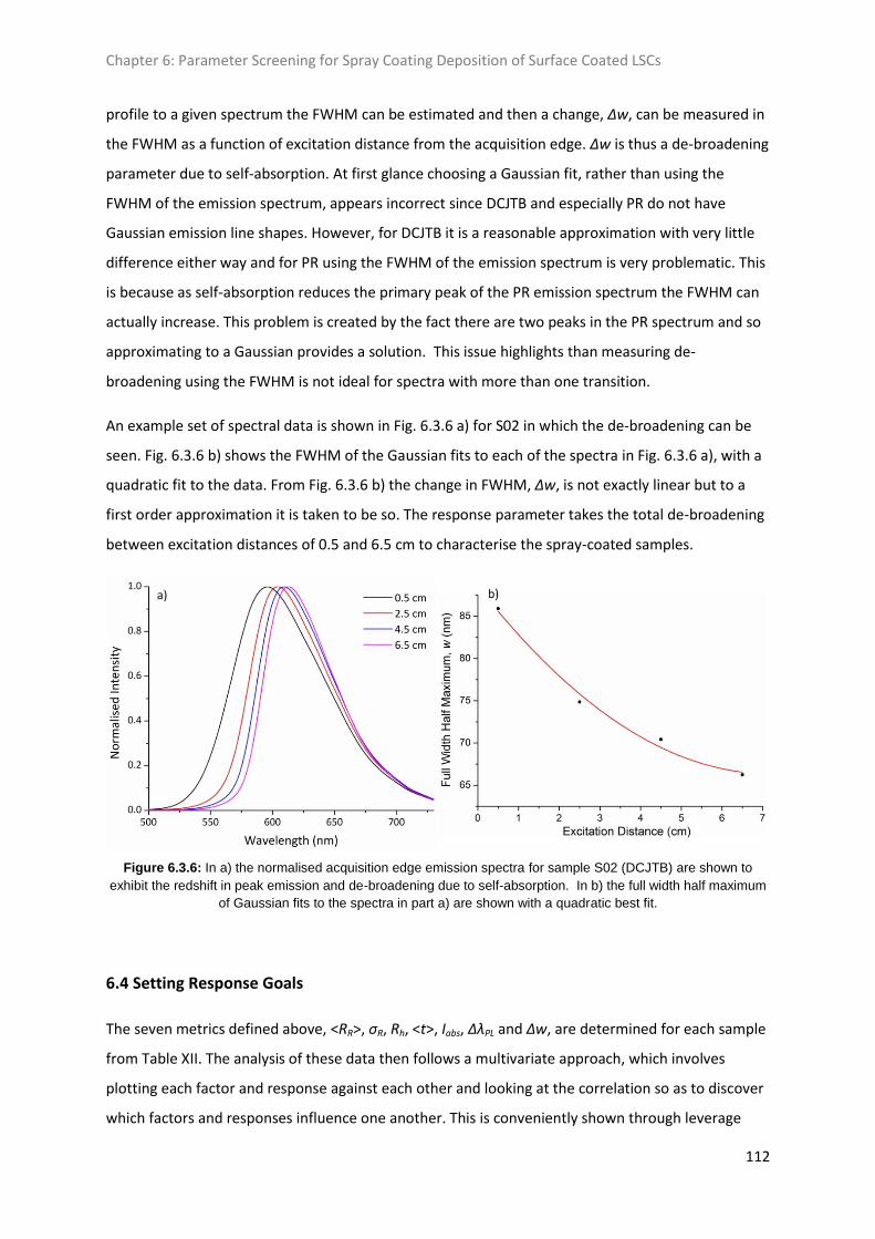
Chapter 6: Parameter Screening for Spray Coating Deposition of Surface Coated LSCs
112
profile to a given spectrum the FWHM can be estimated and then a change, Δw, can be measured in
the FWHM as a function of excitation distance from the acquisition edge. Δw is thus a de-broadening
parameter due to self-absorption. At first glance choosing a Gaussian fit, rather than using the
FWHM of the emission spectrum, appears incorrect since DCJTB and especially PR do not have
Gaussian emission line shapes. However, for DCJTB it is a reasonable approximation with very little
difference either way and for PR using the FWHM of the emission spectrum is very problematic. This
is because as self-absorption reduces the primary peak of the PR emission spectrum the FWHM can
actually increase. This problem is created by the fact there are two peaks in the PR spectrum and so
approximating to a Gaussian provides a solution. This issue highlights than measuring de-
broadening using the FWHM is not ideal for spectra with more than one transition.
An example set of spectral data is shown in Fig. 6.3.6 a) for S02 in which the de-broadening can be
seen. Fig. 6.3.6 b) shows the FWHM of the Gaussian fits to each of the spectra in Fig. 6.3.6 a), with a
quadratic fit to the data. From Fig. 6.3.6 b) the change in FWHM, Δw, is not exactly linear but to a
first order approximation it is taken to be so. The response parameter takes the total de-broadening
between excitation distances of 0.5 and 6.5 cm to characterise the spray-coated samples.
Figure 6.3.6: In a) the normalised acquisition edge emission spectra for sample S02 (DCJTB) are shown to
exhibit the redshift in peak emission and de-broadening due to self-absorption. In b) the full width half maximum
of Gaussian fits to the spectra in part a) are shown with a quadratic best fit.
6.4 Setting Response Goals
The seven metrics defined above, <RR>, σR, Rh, <t>, Iabs, ΔλPL and Δw, are determined for each sample
from Table XII. The analysis of these data then follows a multivariate approach, which involves
plotting each factor and response against each other and looking at the correlation so as to discover
which factors and responses influence one another. This is conveniently shown through leverage
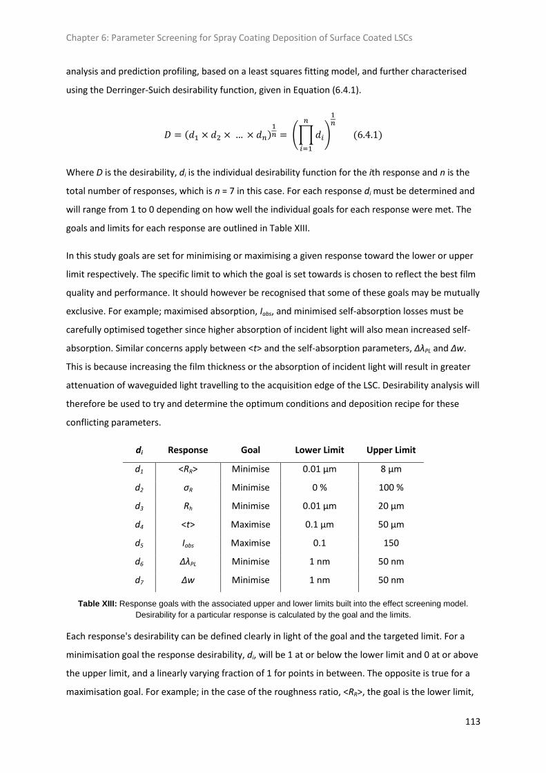
Chapter 6: Parameter Screening for Spray Coating Deposition of Surface Coated LSCs
113
analysis and prediction profiling, based on a least squares fitting model, and further characterised
using the Derringer-Suich desirability function, given in Equation (6.4.1).
Where D is the desirability, di is the individual desirability function for the ith response and n is the
total number of responses, which is n = 7 in this case. For each response di must be determined and
will range from 1 to 0 depending on how well the individual goals for each response were met. The
goals and limits for each response are outlined in Table XIII.
In this study goals are set for minimising or maximising a given response toward the lower or upper
limit respectively. The specific limit to which the goal is set towards is chosen to reflect the best film
quality and performance. It should however be recognised that some of these goals may be mutually
exclusive. For example; maximised absorption, Iabs, and minimised self-absorption losses must be
carefully optimised together since higher absorption of incident light will also mean increased self-
absorption. Similar concerns apply between <t> and the self-absorption parameters, ΔλPL and Δw.
This is because increasing the film thickness or the absorption of incident light will result in greater
attenuation of waveguided light travelling to the acquisition edge of the LSC. Desirability analysis will
therefore be used to try and determine the optimum conditions and deposition recipe for these
conflicting parameters.
di Response Goal Lower Limit Upper Limit
d1 <RR> Minimise 0.01 μm 8 μm
d2 σR Minimise 0 % 100 %
d3 Rh Minimise 0.01 μm 20 μm
d4 <t> Maximise 0.1 μm 50 μm
d5 Iabs Maximise 0.1 150
d6 ΔλPL Minimise 1 nm 50 nm
d7 Δw Minimise 1 nm 50 nm
Table XIII: Response goals with the associated upper and lower limits built into the effect screening model.
Desirability for a particular response is calculated by the goal and the limits.
Each response's desirability can be defined clearly in light of the goal and the targeted limit. For a
minimisation goal the response desirability, di, will be 1 at or below the lower limit and 0 at or above
the upper limit, and a linearly varying fraction of 1 for points in between. The opposite is true for a
maximisation goal. For example; in the case of the roughness ratio, <RR>, the goal is the lower limit,
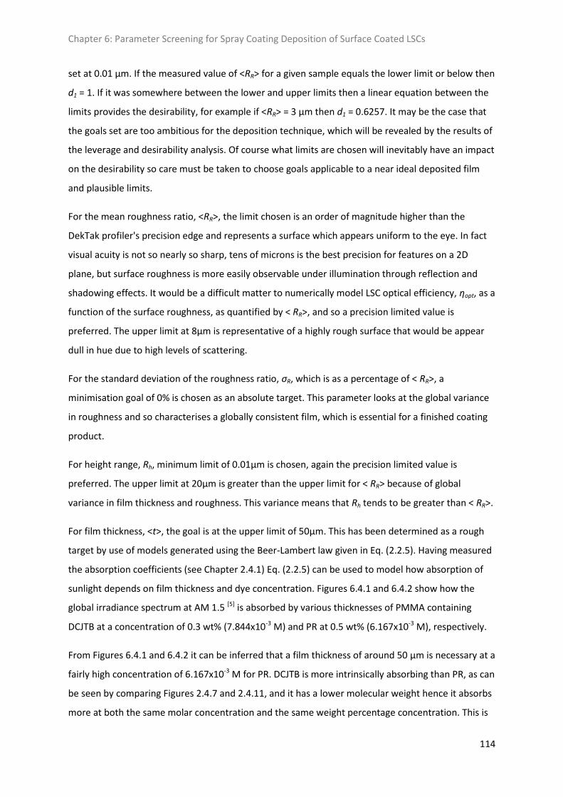
Chapter 6: Parameter Screening for Spray Coating Deposition of Surface Coated LSCs
114
set at 0.01 μm. If the measured value of <RR> for a given sample equals the lower limit or below then
d1 = 1. If it was somewhere between the lower and upper limits then a linear equation between the
limits provides the desirability, for example if <RR> = 3 μm then d1 = 0.6257. It may be the case that
the goals set are too ambitious for the deposition technique, which will be revealed by the results of
the leverage and desirability analysis. Of course what limits are chosen will inevitably have an impact
on the desirability so care must be taken to choose goals applicable to a near ideal deposited film
and plausible limits.
For the mean roughness ratio, <RR>, the limit chosen is an order of magnitude higher than the
DekTak profiler's precision edge and represents a surface which appears uniform to the eye. In fact
visual acuity is not so nearly so sharp, tens of microns is the best precision for features on a 2D
plane, but surface roughness is more easily observable under illumination through reflection and
shadowing effects. It would be a difficult matter to numerically model LSC optical efficiency, ηopt, as a
function of the surface roughness, as quantified by < RR>, and so a precision limited value is
preferred. The upper limit at 8μm is representative of a highly rough surface that would be appear
dull in hue due to high levels of scattering.
For the standard deviation of the roughness ratio, σR, which is as a percentage of < RR>, a
minimisation goal of 0% is chosen as an absolute target. This parameter looks at the global variance
in roughness and so characterises a globally consistent film, which is essential for a finished coating
product.
For height range, Rh, minimum limit of 0.01μm is chosen, again the precision limited value is
preferred. The upper limit at 20μm is greater than the upper limit for < RR> because of global
variance in film thickness and roughness. This variance means that Rh tends to be greater than < RR>.
For film thickness, <t>, the goal is at the upper limit of 50μm. This has been determined as a rough
target by use of models generated using the Beer-Lambert law given in Eq. (2.2.5). Having measured
the absorption coefficients (see Chapter 2.4.1) Eq. (2.2.5) can be used to model how absorption of
sunlight depends on film thickness and dye concentration. Figures 6.4.1 and 6.4.2 show how the
global irradiance spectrum at AM 1.5 [5] is absorbed by various thicknesses of PMMA containing
DCJTB at a concentration of 0.3 wt% (7.844x10⁻³ M) and PR at 0.5 wt% (6.167x10⁻³ M), respectively.
From Figures 6.4.1 and 6.4.2 it can be inferred that a film thickness of around 50 μm is necessary at a
fairly high concentration of 6.167x10⁻³ M for PR. DCJTB is more intrinsically absorbing than PR, as can
be seen by comparing Figures 2.4.7 and 2.4.11, and it has a lower molecular weight hence it absorbs
more at both the same molar concentration and the same weight percentage concentration. This is
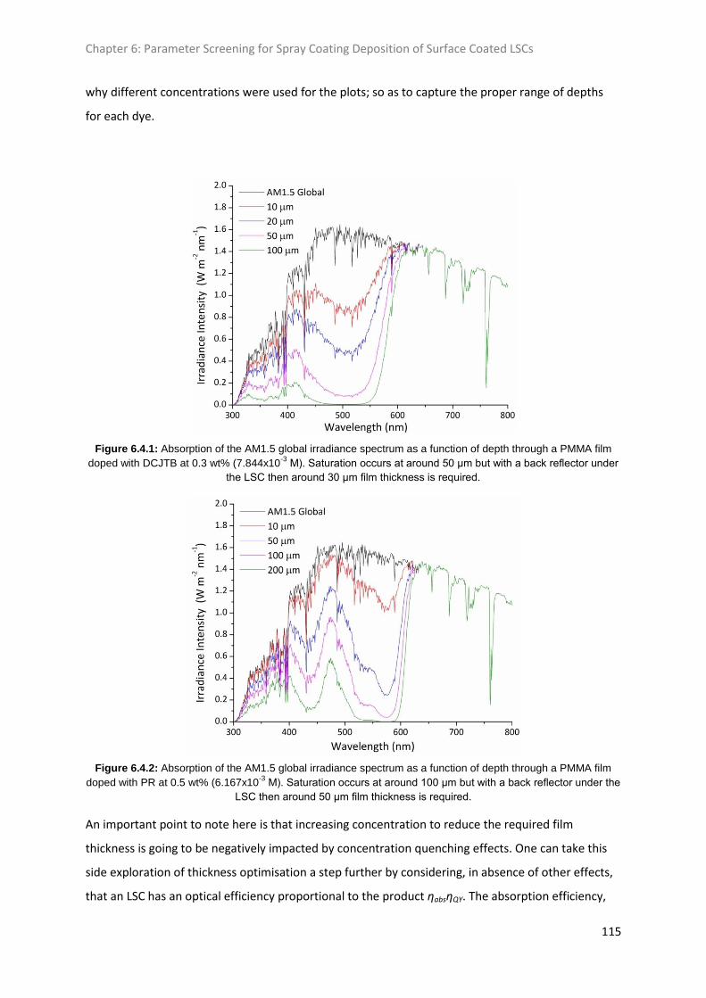
Chapter 6: Parameter Screening for Spray Coating Deposition of Surface Coated LSCs
115
why different concentrations were used for the plots; so as to capture the proper range of depths
for each dye.
Figure 6.4.1: Absorption of the AM1.5 global irradiance spectrum as a function of depth through a PMMA film
doped with DCJTB at 0.3 wt% (7.844x10⁻³
M). Saturation occurs at around 50 μm but with a back reflector under
the LSC then around 30 μm film thickness is required.
Figure 6.4.2: Absorption of the AM1.5 global irradiance spectrum as a function of depth through a PMMA film
doped with PR at 0.5 wt% (6.167x10⁻³
M). Saturation occurs at around 100 μm but with a back reflector under the
LSC then around 50 μm film thickness is required.
An important point to note here is that increasing concentration to reduce the required film
thickness is going to be negatively impacted by concentration quenching effects. One can take this
side exploration of thickness optimisation a step further by considering, in absence of other effects,
that an LSC has an optical efficiency proportional to the product ηabsηQY. The absorption efficiency,
Chapter 6: Parameter Screening for Spray Coating Deposition of Surface Coated LSCs
116
ηabs, for a given film thickness is the integral of the AM1.5 global spectrum minus the same spectrum
after absorption by a given dye and film thickness. By expressing this absorption integral as a
fraction of the total and multiplying by the associated quantum yield, ηQY, one gets an efficiency
estimation for the fluorophores. This enables the optimisation of their properties for thin film LSCs
and as is shown in Fig. 6.4.3 for DCJTB and PR at several concentrations as a function of film
thickness.
Figure 6.4.3: The LSC efficiency estimator, ηabsηQY, is plotted here against film thickness for various
concentrations of DCJTB and PR in PMMA. Weight percentage concentrations are chosen so as to have
comparable molar concentrations; so 0.1 wt% DCJTB is similar to 0.2 wt% PR, 0.3 wt% DCJTB is similar to 0.6
wt% PR and so on.
Fig. 6.4.3 shows PR to be the best dye due to its higher ηQY at a given concentration, though DCJTB
plateaus at lower film thickness due to its higher intrinsic absorption. The figure also reveals, with
careful evaluation, the optimum thicknesses and concentrations to use. The fluorophore
concentration need to be minimised due to reduction of quantum yield by concentration quenching
(see chapter 7). Additionally the film thickness needs to be minimised for the practicalities of
fabrication. For DCJTB a concentration between 0.3 wt% and 0.5 wt% will be ideal with a thickness at
around 30 to 40 μm. As can be seen at this point the absorption has not saturated to a plateau but
with a back reflector it will get close; one can consider a back reflector to essentially double the
effective film thickness. For PR the concentration will be best at around 0.6 wt% at a thickness of 100
μm. Notice how in both cases for DCJTB and PR the circles (0.3 wt% and 0.6 wt% respectively) end up
the highest in collection efficiency as characterised here. This comes about due to the higher
quantum yields, and hence lower concentration quenching, allowing more energy to be harvested
for thicker films. One can see that for film thicknesses well above 200 μm the lowest concentrations
(squares) are likely to reach even higher values of ηabsηQY but such film thicknesses become
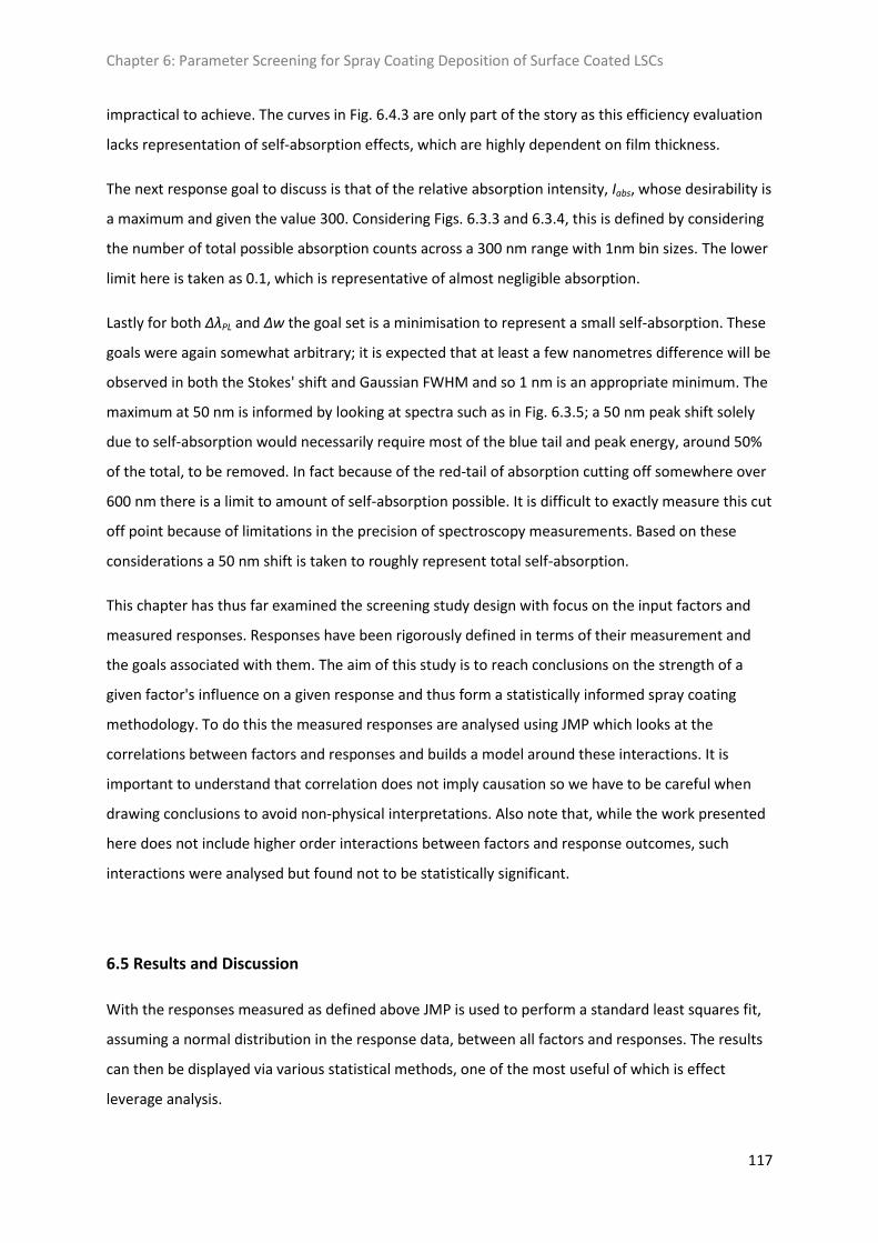
Chapter 6: Parameter Screening for Spray Coating Deposition of Surface Coated LSCs
117
impractical to achieve. The curves in Fig. 6.4.3 are only part of the story as this efficiency evaluation
lacks representation of self-absorption effects, which are highly dependent on film thickness.
The next response goal to discuss is that of the relative absorption intensity, Iabs, whose desirability is
a maximum and given the value 300. Considering Figs. 6.3.3 and 6.3.4, this is defined by considering
the number of total possible absorption counts across a 300 nm range with 1nm bin sizes. The lower
limit here is taken as 0.1, which is representative of almost negligible absorption.
Lastly for both ΔλPL and Δw the goal set is a minimisation to represent a small self-absorption. These
goals were again somewhat arbitrary; it is expected that at least a few nanometres difference will be
observed in both the Stokes' shift and Gaussian FWHM and so 1 nm is an appropriate minimum. The
maximum at 50 nm is informed by looking at spectra such as in Fig. 6.3.5; a 50 nm peak shift solely
due to self-absorption would necessarily require most of the blue tail and peak energy, around 50%
of the total, to be removed. In fact because of the red-tail of absorption cutting off somewhere over
600 nm there is a limit to amount of self-absorption possible. It is difficult to exactly measure this cut
off point because of limitations in the precision of spectroscopy measurements. Based on these
considerations a 50 nm shift is taken to roughly represent total self-absorption.
This chapter has thus far examined the screening study design with focus on the input factors and
measured responses. Responses have been rigorously defined in terms of their measurement and
the goals associated with them. The aim of this study is to reach conclusions on the strength of a
given factor's influence on a given response and thus form a statistically informed spray coating
methodology. To do this the measured responses are analysed using JMP which looks at the
correlations between factors and responses and builds a model around these interactions. It is
important to understand that correlation does not imply causation so we have to be careful when
drawing conclusions to avoid non-physical interpretations. Also note that, while the work presented
here does not include higher order interactions between factors and response outcomes, such
interactions were analysed but found not to be statistically significant.
6.5 Results and Discussion
With the responses measured as defined above JMP is used to perform a standard least squares fit,
assuming a normal distribution in the response data, between all factors and responses. The results
can then be displayed via various statistical methods, one of the most useful of which is effect
leverage analysis.

Chapter 6: Parameter Screening for Spray Coating Deposition of Surface Coated LSCs
118
6.5.1 Effect Leverage Analysis
Effect leverage analysis is performed response by response and looks at the influence of each factor
by plotting the response residuals without the given factor against the response residuals with that
factor included. Thus there are nine leverage plots for each response, too many to display here,
which are usefully combined into a whole model leverage plot where the measured response is
plotted against the predicted response from the least squares model. Figure 6.5.1 shows whole
model leverage plots for the roughness parameters <RR>, σR and Rh.
Figure 6.5.1: Leverage plots of the whole fitted least squares model including each of the nine factors for each of
a) <RR>, b) σR and c) Rh. Data points refer to the measured and predicted response values for each sample, the
dashed-blue line is the y-axis mean for the measured response values, the solid-red line is the least squares fit
and the dashed-red lines are the 5% significance levels. The P value, R2 and RMSE goodness of fit statistics are
also included.
What is immediately clear from Fig. 6.5.1 is that these responses are not significantly influenced by
the chosen factors. The mean roughness ratio <RR> is the best of these with P = 0.086, or over 90%
confidence which is not regarded significant. This is seen by the dashed-red confidence intervals
enclosing the dashed-blue measured response mean. The other goodness of fit statistics further
corroborate this impression from the leverage plots, as shown in Table XIV. One also notices,
particularly for Rh, that the gradients are unstable which is seen by the angle with which the red-
Chapter 6: Parameter Screening for Spray Coating Deposition of Surface Coated LSCs
119
dashed lines depart from least squares fit line. Such instabilities are anathema to a model's
predicting power and come from large sources of unexplained variance.
Why is this the case? It was expected that the roughness of the deposited film would vary more
substantially with the chosen factors, particularly with solvent, T, Ctot, Pin and Ncoat. Despite there
being obvious difference in roughness between samples these results show that it is not possible to
strongly attribute these differences to the chosen factors. It could be concluded from this that
controlling surface roughness, to the limits set in Table XIII, by spray-coating deposition will be very
challenging though there may be other factors that weren't considered here. This does not bode
well for fine tuning the deposition so as to reduce reflection losses at the interface.
Figure 6.5.2 shows leverage plots for the thickness and relative absorption intensity parameters, <t>
and Iabs, respectively. <t> is seen to have a strong dependence on the fitted model which indicates
that there is significant influence on this response from many of the factors. Only the height, h, of
the spray head had a no confidence result and Ncoat, Pin and s are factors with a high significance on
<t>. All other factors had a borderline significance. This is a somewhat trivial result since when more
material is deposited one would expect greater film thickness. More coats, higher pressure and
slower spray head speeds would all be expected to increase film thickness. These relationships do
show the leveraging process is working, which acts as a test of the statistical method; if there was no
significance on <t> then problems with the model would need consideration.
Figure 6.5.2: Leverage plots of the whole fitted least squares model including each of the nine factors for a) <t>
and b) Iabs.
The integrated absorption, Iabs, effect leverage shows significance above the 99.9% confidence
borderline in the model. This comes due to strong confidence in nearly all factors except Ctot and h.
The leverage plots for Iabs by the factors head height, h, and dye concentration, Cdye, are shown in Fig.

Chapter 6: Parameter Screening for Spray Coating Deposition of Surface Coated LSCs
120
6.5.3 to illustrate factors of negligible and strong influence. These factors have the lowest and
highest significance for Iabs, respectively.
Figure 6.5.3: Leverage plots for Iabs against the factors a) Cdye and b) h.
Clearly increased dye concentration has a massive positive effect on the total absorption of incident
radiation from the xenon arc lamp used in the spectrometer. This is to be expected and is a trivial
relationship better described by the Beer-Lambert law. Similarly a strong relationship to the dye
type, because of intrinsic absorption strength, is seen and to be expected. Strong ties with the
thickness parameter also show in the mutually high confidence relations with Ncoat, Pin and s.
Figure 6.5.4 shows leverage plots for the self-absorption parameters, ΔλPL and Δw.
Figure 6.5.4: Leverage plots of the whole fitted least squares model including each of the nine factors for a) ΔλPL
and b) Δw.
The change in Stokes' shift self-absorption parameter, ΔλPL, shows high confidence of above 99% in
the model whereas the de-broadening parameter, Δw, shows a confidence of about 96%. Some
similarities between these two, <t> and Iabs are to be expected in the factors of influence. For ΔλPL
the factors of significance are Ncoat, dye type, Ctot and Cdye whereas for Δw the factors of significance
are Cdye and s. There is a cross over here between ΔλPL, Δw, <t> and Iabs with common factors of
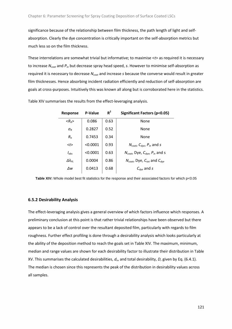
Chapter 6: Parameter Screening for Spray Coating Deposition of Surface Coated LSCs
121
significance because of the relationship between film thickness, the path length of light and self-
absorption. Clearly the dye concentration is critically important on the self-absorption metrics but
much less so on the film thickness.
These interrelations are somewhat trivial but informative; to maximise <t> as required it is necessary
to increase Ncoat and Pin but decrease spray head speed, s. However to minimise self-absorption as
required it is necessary to decrease Ncoat and increase s because the converse would result in greater
film thicknesses. Hence absorbing incident radiation efficiently and reduction of self-absorption are
goals at cross-purposes. Intuitively this was known all along but is corroborated here in the statistics.
Table XIV summarises the results from the effect-leveraging analysis.
Response P-Value R2 Significant Factors (p<0.05)
<RR> 0.086 0.63 None
σR 0.2827 0.52 None
Rh 0.7453 0.34 None
<t> <0.0001 0.93 Ncoat, Cdye, Pin and s
Iabs <0.0001 0.63 Ncoat, Dye, Cdye, Pin and s
ΔλPL 0.0004 0.86 Ncoat, Dye, Ctot and Cdye
Δw 0.0413 0.68 Cdye and s
Table XIV: Whole model best fit statistics for the response and their associated factors for which p<0.05
6.5.2 Desirability Analysis
The effect-leveraging analysis gives a general overview of which factors influence which responses. A
preliminary conclusion at this point is that rather trivial relationships have been observed but there
appears to be a lack of control over the resultant deposited film, particularly with regards to film
roughness. Further effect profiling is done through a desirability analysis which looks particularly at
the ability of the deposition method to reach the goals set in Table XIV. The maximum, minimum,
median and range values are shown for each desirability factor to illustrate their distribution in Table
XV. This summarises the calculated desirabilities, dn, and total desirability, D, given by Eq. (6.4.1).
The median is chosen since this represents the peak of the distribution in desirability values across
all samples.
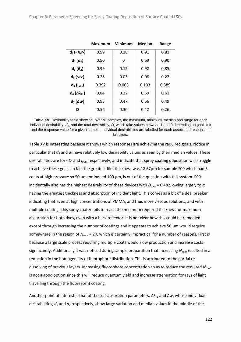
Chapter 6: Parameter Screening for Spray Coating Deposition of Surface Coated LSCs
122
Maximum Minimum Median Range
d1 (<RR>) 0.99 0.18 0.91 0.81
d2 (σR) 0.90 0 0.69 0.90
d3 (Rh) 0.99 0.15 0.92 0.85
d4 (<t>) 0.25 0.03 0.08 0.22
d5 (Iabs) 0.392 0.003 0.103 0.389
d6 (ΔλPL) 0.84 0.22 0.59 0.61
d7 (Δw) 0.95 0.47 0.66 0.49
D 0.56 0.30 0.42 0.26
Table XV: Desirability table showing, over all samples, the maximum, minimum, median and range for each
individual desirability, dn, and the total desirability, D, which take values between 1 and 0 depending on goal limit
and the response value for a given sample. Individual desirabilities are labelled for each associated response in
brackets.
Table XV is interesting because it shows which responses are achieving the required goals. Notice in
particular that d4 and d5 have relatively low desirability values as seen by their median values. These
desirabilities are for <t> and Iabs, respectively, and indicate that spray coating deposition will struggle
to achieve these goals. In fact the greatest film thickness was 12.67μm for sample S09 which had 3
coats at high pressure so 50 μm, or indeed 100 μm, is out of the question with this system. S09
incidentally also has the highest desirability of these devices with Dmax = 0.482, owing largely to it
having the greatest thickness and absorption of incident light. This comes as a bit of a deal breaker
indicating that even at high concentrations of PMMA, and thus more viscous solutions, and with
multiple coatings this spray coater fails to reach the minimum required thickness for maximum
absorption for both dyes, even with a back reflector. It is not clear how this could be remedied
except through increasing the number of coatings and it appears to achieve 50 μm would require
somewhere in the region of Ncoat = 20, which is certainly impractical for a number of reasons. First is
because a large scale process requiring multiple coats would slow production and increase costs
significantly. Additionally it was noticed during sample preparation that increasing Ncoat resulted in a
reduction in the homogeneity of fluorophore distribution. This is attributed to the partial re-
dissolving of previous layers. Increasing fluorophore concentration so as to reduce the required Ncoat
is not a good option since this will reduce quantum yield and increase attenuation for rays of light
travelling through the fluorescent coating.
Another point of interest is that of the self-absorption parameters, ΔλPL and Δw, whose individual
desirabilities, d6 and d7 respectively, show large variation and median values in the middle of the

Chapter 6: Parameter Screening for Spray Coating Deposition of Surface Coated LSCs
123
desirability range. This was understood through the interactions found earlier in the effect leverage
analysis and exhibited in Table XIV; clearly for the ranges of thicknesses produced and dye
concentrations used there is to be significant self-absorption for waveguided light in such an LSC
device. The median average of d6 is 0.59 which corresponds to ΔλPL ≈ 22 nm for light emitted 6cm
from the acquisition edge and this is substantial.
To examine this effect further consider the acquisition edge emission spectrum for S18 and S22 as
shown in Fig. 6.5.5, which have d6 = 0.408 and d6 = 0.572, respectively. In this plot the spectra are
normalised with respect to the spectrum nearest the acquisition edge at 0.5 cm. For DCJTB the
normalisation is done to the intensity of the 0.5 cm spectrum at the peak wavelength of the more
distant spectra. For PR all normalisations for the more distant spectra are on the shoulder at 650 nm.
These normalisations provide an estimation of the relative spectral areas based solely on the red-
shift in emission energy due to self-absorption. This operation is not ideal as the red tails should
overlap, but as an estimator it suffices.
Figure 6.5.5: Sample acquisition edge emission spectra for a) S22 (DCJTB) and b) S18 (PR). For a)
normalisation is done to the intensity of the near edge spectrum at the peak wavelength of the others. For b)
normalisation is done on the shoulder at 650 nm. Intensity integrals are included showing an estimated 35%
(DCJTB) to 38% (PR) total drop in collected energy.
So on average, over a 6cm distance to the acquisition edge, 35-38% of the collected energy is
expected to be lost to self-absorption, the true figure is slightly more. PR suffers this effect more
over shorter distances, which can seen by considering the differences between S18 and S22 via Table
XII and Figs. 6.3.3 and 6.3.4. S22 is actually thinner but has a significantly higher concentration of
DCJTB molecules than PR in S18. Hence S22 actually absorbs more incident light but this analysis
shows that S18 suffers slightly higher self-absorption than S22, and therefore PR suffers more over
shorter distances than DCJTB. Of course some self-absorbed light is re-emitted and trapped again by
TIR, as was explored more thoroughly in the last chapter, but it still represents a severe loss mode
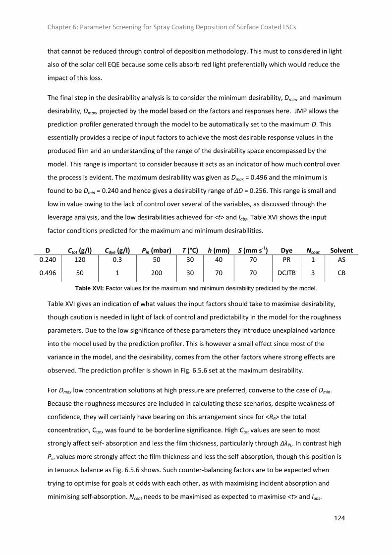
Chapter 6: Parameter Screening for Spray Coating Deposition of Surface Coated LSCs
124
that cannot be reduced through control of deposition methodology. This must to considered in light
also of the solar cell EQE because some cells absorb red light preferentially which would reduce the
impact of this loss.
The final step in the desirability analysis is to consider the minimum desirability, Dmin, and maximum
desirability, Dmax, projected by the model based on the factors and responses here. JMP allows the
prediction profiler generated through the model to be automatically set to the maximum D. This
essentially provides a recipe of input factors to achieve the most desirable response values in the
produced film and an understanding of the range of the desirability space encompassed by the
model. This range is important to consider because it acts as an indicator of how much control over
the process is evident. The maximum desirability was given as Dmax = 0.496 and the minimum is
found to be Dmin = 0.240 and hence gives a desirability range of ΔD = 0.256. This range is small and
low in value owing to the lack of control over several of the variables, as discussed through the
leverage analysis, and the low desirabilities achieved for <t> and Iabs. Table XVI shows the input
factor conditions predicted for the maximum and minimum desirabilities.
D Ctot (g/l) Cdye (g/l) Pin (mbar) T (°C) h (mm) S (mm s-1) Dye Ncoat Solvent
0.240 120 0.3 50 30 40 70 PR 1 AS
0.496 50 1 200 30 70 70 DCJTB 3 CB
Table XVI: Factor values for the maximum and minimum desirability predicted by the model.
Table XVI gives an indication of what values the input factors should take to maximise desirability,
though caution is needed in light of lack of control and predictability in the model for the roughness
parameters. Due to the low significance of these parameters they introduce unexplained variance
into the model used by the prediction profiler. This is however a small effect since most of the
variance in the model, and the desirability, comes from the other factors where strong effects are
observed. The prediction profiler is shown in Fig. 6.5.6 set at the maximum desirability.
For Dmax low concentration solutions at high pressure are preferred, converse to the case of Dmin.
Because the roughness measures are included in calculating these scenarios, despite weakness of
confidence, they will certainly have bearing on this arrangement since for <RR> the total
concentration, Ctot, was found to be borderline significance. High Ctot values are seen to most
strongly affect self- absorption and less the film thickness, particularly through ΔλPL. In contrast high
Pin values more strongly affect the film thickness and less the self-absorption, though this position is
in tenuous balance as Fig. 6.5.6 shows. Such counter-balancing factors are to be expected when
trying to optimise for goals at odds with each other, as with maximising incident absorption and
minimising self-absorption. Ncoat needs to be maximised as expected to maximise <t> and Iabs.
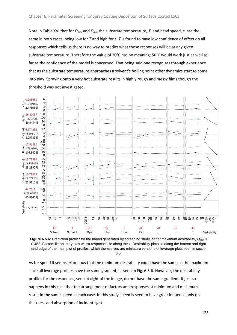
Chapter 6: Parameter Screening for Spray Coating Deposition of Surface Coated LSCs
125
Note in Table XVI that for Dmax and Dmin the substrate temperature, T, and head speed, s, are the
same in both cases, being low for T and high for s. T is found to have low confidence of effect on all
responses which tells us there is no way to predict what those responses will be at any given
substrate temperature. Therefore the value of 30°C has no meaning; 50°C would work just as well as
far as the confidence of the model is concerned. That being said one recognises through experience
that as the substrate temperature approaches a solvent's boiling point other dynamics start to come
into play. Spraying onto a very hot substrate results in highly rough and messy films though the
threshold was not investigated.
Figure 6.5.6: Prediction profiler for the model generated by screening study, set at maximum desirability, Dmax =
0.482. Factors lie on the y-axis whilst responses lie along the x. Desirability plots lie along the bottom and right
hand edge of the main plot of profiles, which themselves are miniature versions of leverage plots seen in section
6.5.
As for speed it seems erroneous that the minimum desirability could have the same as the maximum
since all leverage profiles have the same gradient, as seen in Fig. 6.5.6. However, the desirability
profiles for the responses, seen at right of the image, do not have the same gradient. It just so
happens in this case that the arrangement of factors and responses at minimum and maximum
result in the same speed in each case. In this study speed is seen to have great influence only on
thickness and absorption of incident light.
Chapter 6: Parameter Screening for Spray Coating Deposition of Surface Coated LSCs
126
The choice of solvent was expected to show more interesting influence and so it is surprising to see
that it has only near borderline significance of effect in any response leverage plots. The greatest
effect on a response was for <t> with near borderline significance at 91.8% confidence and saw
toluene as providing greatest thickness. s also shows confidence of 89.3% with the roughness ratio
but in this time with anisole being more desirable with lowest <RR> values. Such a predictions hold
too much uncertainty for definitive statement however, and so does statement that chlorobenzene
proves better than anisole as Table XVI suggests.
For choice of dye and Cdye the model indicates that DCJTB and higher concentration provide the
optimum desirability, but it is absent considerations of concentration quenching of quantum yield,
self-absorption effects and photochemical molecular stability. The model considers DCJTB to be the
best because of its higher intrinsic absorption which has great impact on the relative absorption
intensities, as seen by comparing Figures 6.3.3 and 6.3.4. Dye type also is seen to have a significant
influence, at 99.4% confidence, on the peak shift due to self-absorption, ΔλPL. The leverage analysis
indicates that the least squares mean for DCJTB is at ΔλPL = 18.5 ± 1.3 nm and for PR it is ΔλPL = 24.7 ±
1.3 nm. So based on this model, at high confidence, DCJTB is expected to have significantly lower
self-absorption than PR. This makes sense considering DCJTB has a broader spectrum with a larger
Stokes' shift, as seen comparing Fig. 2.4.7 and 2.4.11. Also consider that the spectrum of PR is
composed of two main transitions where the first of which is largest and lies in the red tail of the
absorption spectrum. Much of this larger component can be consumed by self-absorption over
relatively short distances, as has been seen for DCJTB in Fig.6.5.5. PR does however exhibit higher
quantum yield than DCJTB at all concentrations which, as Fig. 6.4.3 has shown, can improve the
collection efficiency of light. Furthermore PR has much greater photochemical stability with over
80% of the original efficiency remaining after a year long exposure [6], whereas DCM class
fluorophores are known to have low stability.
6.6 Conclusions
The screening design has found success in its ability to assess to value of the spray coating
deposition of LSC bi-layer devices using the Prism Ultra-Coat 300. The clear conclusion based on the
defined response parameters, and their goals set in the desirability analysis, is that this spray coating
system cannot achieve the thicknesses of film required and that the surface roughness cannot be
controlled at all in the range of parameter space explored. Furthermore optimal absorption of
incident light, which cannot be achieved due to the thickness problem, necessitates strong self-
Chapter 6: Parameter Screening for Spray Coating Deposition of Surface Coated LSCs
127
absorption effects over the range of several cm, even with a back reflector considered to reduce
necessary thickness.
The model predicts PR to suffer more from the self-absorption phenomenon than DCJTB which is
supported by considering the spectra of these dyes. The self-absorbed energy in a DCJTB sample
with average change in peak wavelength over 6 cm excitation difference is crudely estimated to be
around 35% based on measured spectra. This shows that self-absorption is strong in these bi-layer
devices which may be exacerbated by longer path lengths due unfavourable scattering from a rough
reflection interface.
6.7 References
[1] K. R. McIntosh, N. Yamada and B. S. Richards, Theoretical Comparison of Cylindrical and Square-
Planar Luminescent Solar Concentrators, App. Phys. B 88, 285-290 (2007)
[2] G. Colantuono, A. Buckley and R. Erdélyi, Ray-Optics Modelling of Rectangular and Cylindrical 2-
Layer Solar Concentrators, J. Light. Tech. 31, 7, 1033 – 1044 (2013)
[3] A. von Eye, P. Mair and E. Y. Mun, Advances in Configural Frequency Analysis, 3rd ed. (Guilford
Press, USA, 2010), Chap. 12, pp. 223–226.
[4] JMP® 8 Design of Experiments Guide, 2nd ed. (SAS Institute Inc., Cary, NC, USA, 2009), Chap. 2
[5] American Society for Testing and Materials (ASTM), ASTM G173-03 Tables, AM 1.5 Solar
Irradiance Reference Spectrum, http://rredc.nrel.gov/solar/spectra/am1.5/
[6] W. G. J. H. M. van Sark et. al., Luminescent Solar Concentrators - A Review of Recent Results, Opt.
Exp. 16, 26, 21773 (2008)

Chapter 7: Concentration Quenching Effects for Organic Fluorophores in the Solid State
128
Chapter 7
Solid State Concentration Quenching Effects for Organic
Fluorophores and Implications for LSC Devices
7.1 Introduction
This chapter reviews a series of results exploring concentration quenching effects in organic
fluorophores in the solid state so as to consider the impacts this loss mechanism will have on LSC
optical efficiency. Concentration quenching is a phenomenon observed with all small molecular
fluorescent materials where increased concentration results in diminished fluorescence efficiency, as
briefly discussed in chapter 2.4. When the term concentration quenching of fluorescence is used
what is really being discussed is a change in the balance of radiative and non-radiative transition
decay rates, and from this an inverse relationship between fluorescence quantum yield and
fluorophore concentration. From Eq. (2.4.1) the quantum yield is understood in terms of the ratio of
radiative decay rate to the sum of all transition rates. Therefore through both quantum yield
measurements (chapter 3.1) and fluorescence lifetime measurements (Chapter 3.5), as a function of
fluorophore concentration, ηQY(Cdye) and τ(Cdye), the influence of concentration quenching can be
explored and quantified.
Explored in this chapter are measurements on samples consisting of single fluorophores doped into
solid polymer hosts. The effect of host type, fluorophore concentration and fluorophore type are all
explored in some detail throughout section 7.2. Quantum yield combined with fluorescence lifetime
data using Eq. (2.4.1) allows the concentration quenching effect to be quantified in two
fluorophores, DCM and C102, in sections 7.3 and 7.4, respectively. These data were not available for
PR or the other fluorophores as it was taken early in my research when thought was not given in
preference of particular fluorophores.
The exact mechanism of concentration quenching depends on the system being studied. Dipole-
dipole deactivation interactions between neighbouring fluorophores have been demonstrated in the
solid state for Iridium based phosphor complexes [1]. In this case an r-6 dependence on fluorophore
separation is observed as predicted by Förster in the case of two interacting point-like dipoles. In
reality the approximation of point-like dipoles may not hold, for example in solid state polymer
blends where point-surface or surface-surface interactions may occur. In such cases the dependence

Chapter 7: Concentration Quenching Effects for Organic Fluorophores in the Solid State
129
on fluorophore separation could be of r-3 or r-2 [2, 3], respectively. Exciplex formation [4] and the
presence of quenching agents [5] have also been identified as forms of quenching in particular cases.
Concentration quenching of fluorescence is therefore the result of a number of mechanisms that act
to reduce the fluorescent emission efficiency of a particular transition of interest. What mechanisms
are actually present will depend on the local environment of the fluorophore, so host properties will
be important, and also on the chemical and photophysical properties of the fluorophore itself. It
therefore may or may not be possible to discern the nature of the quenching in the case of DCM and
C102.
All samples are fabricated by first preparing a stock solutions of host materials in chlorobenzene, or
chloroform for polycarbonate (PC), at Chost = 250 g/l. Blends are made with stock solutions of
fluorophores in chlorobenzene or chloroform at Cdye = 2 g/l or 0.05 g/l. Fluorophore stock solutions
of different Cdye values are needed to achieve dye concentrations in the resultant thin film in the
range 1x10⁻⁴ M < Cdye < 0.1 M. Deposition occurs onto glass substrates by spin coating at 1000 rpm
giving films of thickness in the range (350 < x < 600) ± 30 nm.
7.2 The Impact of Host Material on Fluorescence
This first results section qualitatively explores a selection of results looking at how different host and
fluorescent materials interact and how the fluorescence is affected. Fig. 7.2.1 shows ηQY for a
number fluorophores doped in PMMA plotted as a function fluorophore concentration, Cdye.
Figure 7.2.1: Plot of quantum yield against dye concentration for PMMA doped with various fluorophores
including three DCM class dyes (green), three perylene based dyes (red), R6G (magenta) and C102 (blue).
These fluorophores have spectra and chemical structures exhibited in chapter 2.4.1. Lines are a guide to the eye.
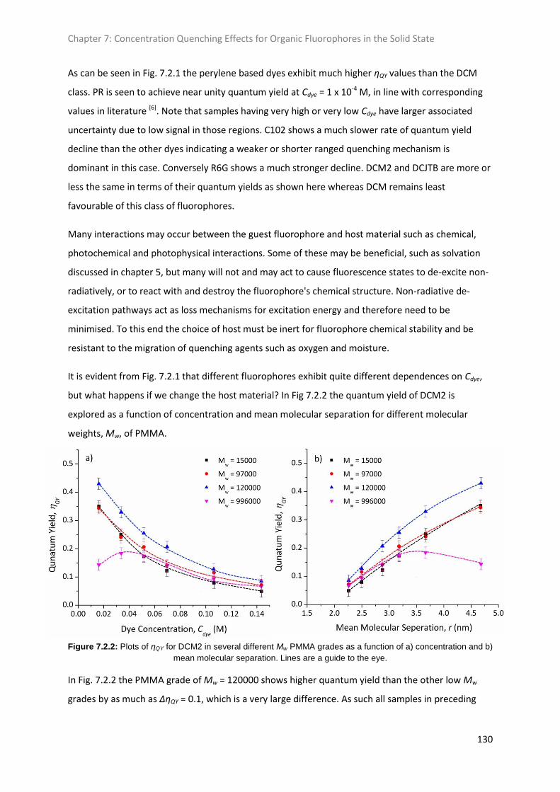
Chapter 7: Concentration Quenching Effects for Organic Fluorophores in the Solid State
130
As can be seen in Fig. 7.2.1 the perylene based dyes exhibit much higher ηQY values than the DCM
class. PR is seen to achieve near unity quantum yield at Cdye = 1 x 10⁻⁴ M, in line with corresponding
values in literature [6]. Note that samples having very high or very low Cdye have larger associated
uncertainty due to low signal in those regions. C102 shows a much slower rate of quantum yield
decline than the other dyes indicating a weaker or shorter ranged quenching mechanism is
dominant in this case. Conversely R6G shows a much stronger decline. DCM2 and DCJTB are more or
less the same in terms of their quantum yields as shown here whereas DCM remains least
favourable of this class of fluorophores.
Many interactions may occur between the guest fluorophore and host material such as chemical,
photochemical and photophysical interactions. Some of these may be beneficial, such as solvation
discussed in chapter 5, but many will not and may act to cause fluorescence states to de-excite non-
radiatively, or to react with and destroy the fluorophore's chemical structure. Non-radiative de-
excitation pathways act as loss mechanisms for excitation energy and therefore need to be
minimised. To this end the choice of host must be inert for fluorophore chemical stability and be
resistant to the migration of quenching agents such as oxygen and moisture.
It is evident from Fig. 7.2.1 that different fluorophores exhibit quite different dependences on Cdye,
but what happens if we change the host material? In Fig 7.2.2 the quantum yield of DCM2 is
explored as a function of concentration and mean molecular separation for different molecular
weights, Mw, of PMMA.
Figure 7.2.2: Plots of ηQY for DCM2 in several different Mw PMMA grades as a function of a) concentration and b)
mean molecular separation. Lines are a guide to the eye.
In Fig. 7.2.2 the PMMA grade of Mw = 120000 shows higher quantum yield than the other low Mw
grades by as much as ΔηQY = 0.1, which is a very large difference. As such all samples in preceding
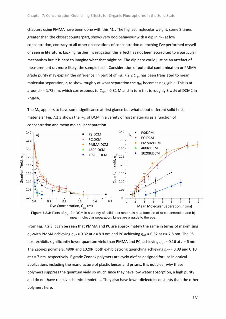
Chapter 7: Concentration Quenching Effects for Organic Fluorophores in the Solid State
131
chapters using PMMA have been done with this Mw. The highest molecular weight, some 8 times
greater than the closest counterpart, shows very odd behaviour with a dip in ηQY at low
concentration, contrary to all other observations of concentration quenching I've performed myself
or seen in literature. Lacking further investigation this effect has not been accredited to a particular
mechanism but it is hard to imagine what that might be. The dip here could just be an artefact of
measurement or, more likely, the sample itself. Consideration of potential contamination or PMMA
grade purity may explain the difference. In part b) of Fig. 7.2.2 Cdye has been translated to mean
molecular separation, r, to show roughly at what separation the ηQY becomes negligible. This is at
around r = 1.75 nm, which corresponds to Cdye = 0.31 M and in turn this is roughly 8 wt% of DCM2 in
PMMA.
The Mw appears to have some significance at first glance but what about different solid host
materials? Fig. 7.2.3 shows the ηQY of DCM in a variety of host materials as a function of
concentration and mean molecular separation.
Figure 7.2.3: Plots of ηQY for DCM in a variety of solid host materials as a function of a) concentration and b)
mean molecular separation. Lines are a guide to the eye.
From Fig. 7.2.3 it can be seen that PMMA and PC are approximately the same in terms of maximising
ηQY with PMMA achieving ηQY = 0.32 at r = 8.9 nm and PC achieving ηQY = 0.32 at r = 7.8 nm. The PS
host exhibits significantly lower quantum yield than PMMA and PC, achieving ηQY = 0.16 at r = 6 nm.
The Zeonex polymers, 480R and 1020R, both exhibit strong quenching achieving ηQY = 0.09 and 0.10
at r = 7 nm, respectively. R grade Zeonex polymers are cyclo olefins designed for use in optical
applications including the manufacture of plastic lenses and prisms. It is not clear why these
polymers suppress the quantum yield so much since they have low water absorption, a high purity
and do not have reactive chemical moieties. They also have lower dielectric constants than the other
polymers here.

Chapter 7: Concentration Quenching Effects for Organic Fluorophores in the Solid State
132
From plot b) in Fig. 7.2.3 the mean r for negligible ηQY is roughly the same as in the case of DCM2 in
Fig. 7.2.2. It is hard to be clearer because only one set of data for PMMA is present and the other
polymers appear to also differ in this respect.
PMMA stands out as the best material in light of processibility but has a lower refractive index than
PC. Going back to the LSC optical efficiency considerations of chapter 2.2, pages 13 - 17, higher
refractive indices reduce transmission efficiency, ηfr, but increase trapping efficiency, ηtrap. We also
learnt in chapter 5, page 76, that increasing refractive index would reduce the influence of solvation
for a fixed value of relative permittivity. It is through this balance of efficiencies that the choice
between PMMA and PC must be made, which is summarised for the product ηfrηtrap in Fig. 2.2.4. A
further consideration is the host absorption coefficients across the visible spectrum; Table IV shows
PMMA to be considerably better than PC in this property.
Finally in this exploration of different solid host materials two other forms of acrylic polymer,
poly(butyl methacrylate) (PBMA) and poly(cyclohexyl methacrylate) (PCHMA), are compared to
PMMA. These polymers were chosen due to their similarities to PMMA and availability from Sigma
Aldrich. In Fig 7.2.4 the fluorescence lifetime of DCM is plotted against log10 of concentration for
these three acrylic polymers.
Figure 7.2.4: Fluorescence lifetime is plotted here against log10 of DCM concentration for three solid acrylic
hosts; PMMA, PBMA and PCHMA.
Fig. 7.2.4 shows a significant difference in the lifetime of the fluorescence state at low
concentrations. This does not necessarily translate to PMMA having a greater quantum yield since
the measured lifetime, τ, is the inverse of the sum of all excited state decay rates. Hence if either the
radiative rate or non-radiative rate decrease then the lifetime with increase. PBMA shows no
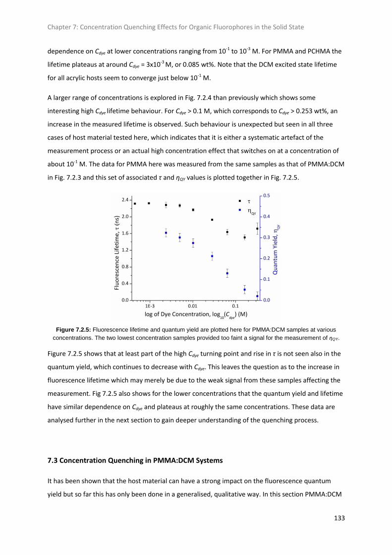
Chapter 7: Concentration Quenching Effects for Organic Fluorophores in the Solid State
133
dependence on Cdye at lower concentrations ranging from 10-1 to 10-3 M. For PMMA and PCHMA the
lifetime plateaus at around Cdye = 3x10⁻³ M, or 0.085 wt%. Note that the DCM excited state lifetime
for all acrylic hosts seem to converge just below 10-1 M.
A larger range of concentrations is explored in Fig. 7.2.4 than previously which shows some
interesting high Cdye lifetime behaviour. For Cdye > 0.1 M, which corresponds to Cdye > 0.253 wt%, an
increase in the measured lifetime is observed. Such behaviour is unexpected but seen in all three
cases of host material tested here, which indicates that it is either a systematic artefact of the
measurement process or an actual high concentration effect that switches on at a concentration of
about 10-1 M. The data for PMMA here was measured from the same samples as that of PMMA:DCM
in Fig. 7.2.3 and this set of associated τ and ηQY values is plotted together in Fig. 7.2.5.
Figure 7.2.5: Fluorescence lifetime and quantum yield are plotted here for PMMA:DCM samples at various
concentrations. The two lowest concentration samples provided too faint a signal for the measurement of ηQY.
Figure 7.2.5 shows that at least part of the high Cdye turning point and rise in τ is not seen also in the
quantum yield, which continues to decrease with Cdye. This leaves the question as to the increase in
fluorescence lifetime which may merely be due to the weak signal from these samples affecting the
measurement. Fig 7.2.5 also shows for the lower concentrations that the quantum yield and lifetime
have similar dependence on Cdye and plateaus at roughly the same concentrations. These data are
analysed further in the next section to gain deeper understanding of the quenching process.
7.3 Concentration Quenching in PMMA:DCM Systems
It has been shown that the host material can have a strong impact on the fluorescence quantum
yield but so far this has only been done in a generalised, qualitative way. In this section PMMA:DCM

Chapter 7: Concentration Quenching Effects for Organic Fluorophores in the Solid State
134
samples are analysed further to attempt to quantify the concentration quenching mechanism and
determine its dependence on mean molecular separation, r. This dependence will give insight into
the quenching mechanism as it defines the strength or range of its effect. A pertinent example is
Förster Resonant Energy Transfer (FRET) based point-like dipole-dipole interactions which have a
rate, kFRET, with a r-6 dependence as given by Eq. (7.3.1).
Where τ0 the intrinsic decay lifetime of the fluorescent state and r0 is the Förster radius for
interacting point-like dipoles at which FRET efficiency is 50%. For point-surface interactions, as
developed in J. Cabanillas-Gonzalez et. al. 2004[2], this rate equation becomes that of Eq. (7.3.2) for
kET;
Where ṟ0 is the Förster radius for point-surface interaction related to r0 by Eq. (7.3.3) in which ρ is
the donor fluorophore density; in this case this is the same as the fluorophore density as the
interaction is between same species fluorophores. To determine the dependence of the
concentration quenching rate, kQ, on r we turn back to the data exhibited in Fig. 7.2.5, but now only
consider the values for Cdye < 0.1 M. This is shown with exponential best fit curves in Fig. 7.3.1.
Figure 7.3.1: Double-y plot showing fluorescence lifetime and quantum yield as a function of mean molecular
separation for PMMA:DCM films. Best fit curves are exponential decay fits extrapolated to the intercept.
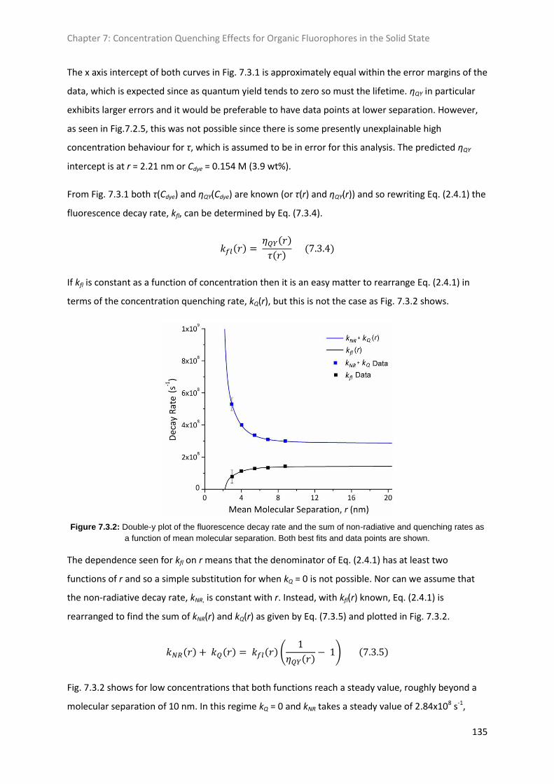
Chapter 7: Concentration Quenching Effects for Organic Fluorophores in the Solid State
135
The x axis intercept of both curves in Fig. 7.3.1 is approximately equal within the error margins of the
data, which is expected since as quantum yield tends to zero so must the lifetime. ηQY in particular
exhibits larger errors and it would be preferable to have data points at lower separation. However,
as seen in Fig.7.2.5, this was not possible since there is some presently unexplainable high
concentration behaviour for τ, which is assumed to be in error for this analysis. The predicted ηQY
intercept is at r = 2.21 nm or Cdye = 0.154 M (3.9 wt%).
From Fig. 7.3.1 both τ(Cdye) and ηQY(Cdye) are known (or τ(r) and ηQY(r)) and so rewriting Eq. (2.4.1) the
fluorescence decay rate, kfl, can be determined by Eq. (7.3.4).
If kfl is constant as a function of concentration then it is an easy matter to rearrange Eq. (2.4.1) in
terms of the concentration quenching rate, kQ(r), but this is not the case as Fig. 7.3.2 shows.
Figure 7.3.2: Double-y plot of the fluorescence decay rate and the sum of non-radiative and quenching rates as
a function of mean molecular separation. Both best fits and data points are shown.
The dependence seen for kfl on r means that the denominator of Eq. (2.4.1) has at least two
functions of r and so a simple substitution for when kQ = 0 is not possible. Nor can we assume that
the non-radiative decay rate, kNR, is constant with r. Instead, with kfl(r) known, Eq. (2.4.1) is
rearranged to find the sum of kNR(r) and kQ(r) as given by Eq. (7.3.5) and plotted in Fig. 7.3.2.
Fig. 7.3.2 shows for low concentrations that both functions reach a steady value, roughly beyond a
molecular separation of 10 nm. In this regime kQ = 0 and kNR takes a steady value of 2.84x10⁸ s-1,
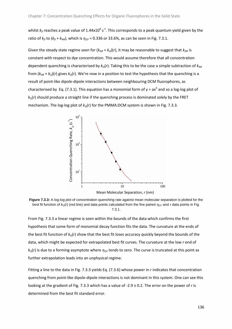
Chapter 7: Concentration Quenching Effects for Organic Fluorophores in the Solid State
136
whilst kfl reaches a peak value of 1.44x10⁸ s-1. This corresponds to a peak quantum yield given by the
ratio of kfl to (kfl + kNR), which is ηQY = 0.336 or 33.6%, as can be seen in Fig. 7.3.1.
Given the steady state regime seen for (kNR + kQ)(r), it may be reasonable to suggest that kNR is
constant with respect to dye concentration. This would assume therefore that all concentration
dependent quenching is characterised by kQ(r). Taking this to be the case a simple subtraction of kNR
from (kNR + kQ)(r) gives kQ(r). We're now in a position to test the hypothesis that the quenching is a
result of point-like dipole-dipole interactions between neighbouring DCM fluorophores, as
characterised by Eq. (7.3.1). This equation has a monomial form of y = axb and so a log-log plot of
kQ(r) should produce a straight line if the quenching process is dominated solely by the FRET
mechanism. The log-log plot of kQ(r) for the PMMA:DCM system is shown in Fig. 7.3.3.
Figure 7.3.3: A log-log plot of concentration quenching rate against mean molecular separation is plotted for the
best fit function of kQ(r) (red line) and data points calculated from the five paired ηQY and τ data points in Fig.
7.3.1.
From Fig. 7.3.3 a linear regime is seen within the bounds of the data which confirms the first
hypothesis that some form of monomial decay function fits the data. The curvature at the ends of
the best fit function of kQ(r) show that the best fit loses accuracy quickly beyond the bounds of the
data, which might be expected for extrapolated best fit curves. The curvature at the low r end of
kQ(r) is due to a forming asymptote where ηQY tends to zero. The curve is truncated at this point as
further extrapolation leads into an unphysical regime.
Fitting a line to the data in Fig. 7.3.3 yields Eq. (7.3.6) whose power in r indicates that concentration
quenching from point-like dipole-dipole interactions is not dominant in this system. One can see this
looking at the gradient of Fig. 7.3.3 which has a value of -2.9 ± 0.2. The error on the power of r is
determined from the best fit standard error.
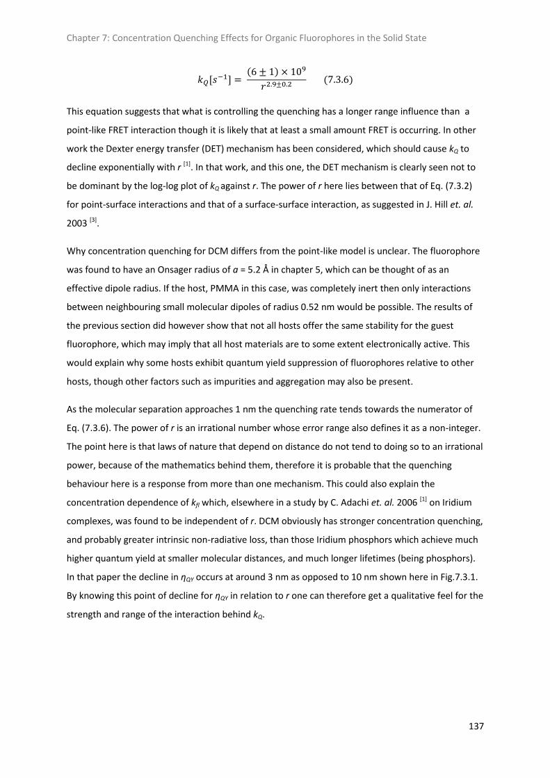
Chapter 7: Concentration Quenching Effects for Organic Fluorophores in the Solid State
137
This equation suggests that what is controlling the quenching has a longer range influence than a
point-like FRET interaction though it is likely that at least a small amount FRET is occurring. In other
work the Dexter energy transfer (DET) mechanism has been considered, which should cause kQ to
decline exponentially with r [1]. In that work, and this one, the DET mechanism is clearly seen not to
be dominant by the log-log plot of kQ against r. The power of r here lies between that of Eq. (7.3.2)
for point-surface interactions and that of a surface-surface interaction, as suggested in J. Hill et. al.
2003 [3].
Why concentration quenching for DCM differs from the point-like model is unclear. The fluorophore
was found to have an Onsager radius of a = 5.2 Å in chapter 5, which can be thought of as an
effective dipole radius. If the host, PMMA in this case, was completely inert then only interactions
between neighbouring small molecular dipoles of radius 0.52 nm would be possible. The results of
the previous section did however show that not all hosts offer the same stability for the guest
fluorophore, which may imply that all host materials are to some extent electronically active. This
would explain why some hosts exhibit quantum yield suppression of fluorophores relative to other
hosts, though other factors such as impurities and aggregation may also be present.
As the molecular separation approaches 1 nm the quenching rate tends towards the numerator of
Eq. (7.3.6). The power of r is an irrational number whose error range also defines it as a non-integer.
The point here is that laws of nature that depend on distance do not tend to doing so to an irrational
power, because of the mathematics behind them, therefore it is probable that the quenching
behaviour here is a response from more than one mechanism. This could also explain the
concentration dependence of kfl which, elsewhere in a study by C. Adachi et. al. 2006 [1] on Iridium
complexes, was found to be independent of r. DCM obviously has stronger concentration quenching,
and probably greater intrinsic non-radiative loss, than those Iridium phosphors which achieve much
higher quantum yield at smaller molecular distances, and much longer lifetimes (being phosphors).
In that paper the decline in ηQY occurs at around 3 nm as opposed to 10 nm shown here in Fig.7.3.1.
By knowing this point of decline for ηQY in relation to r one can therefore get a qualitative feel for the
strength and range of the interaction behind kQ.

Chapter 7: Concentration Quenching Effects for Organic Fluorophores in the Solid State
138
7.4 Concentration Quenching in PMMA:C102 Systems
Now follows an identical analysis to that above in section 7.3 for DCM but for C102, which was seen
in Fig. 7.2.1 to show a significantly slower decline in ηQY with Cdye. The fluorescent lifetime and
quantum yield for PMMA:C102 samples, with exponential best fits, are shown in Fig. 7.4.1 as a
function of mean molecular separation. This time, to avoid τ being non-zero when ηQY = 0, the fit for
τ is constrained to the x-axis intercept for ηQY(r).
Comparing Fig. 7.3.1 and 7.4.1 the point at which ηQY begins to decline also differs; for C102 it is
around 5 nm whereas for DCM it is around 10 nm. From the study by C. Adachi et. al. 2006 [1] we saw
iridium phosphors had a plateau value at around 3 nm. Already then one can guess that the C102
concentration quenching rate, kQ, will not be dominated by a FRET based quenching mechanism as
with the phosphors. It must be a shorter range effect than DCM but longer than the phosphors,
obeying a power law in r whose exponent lies in between -6 and -2.61.
Figure 7.4.1: Double-y plot showing fluorescence lifetime and quantum yield as a function of mean molecular
separation for PMMA:C102 films. Best fit curves are exponential decay fits.
From Fig. 7.4.1 the lifetime and quantum yield are known as a function of molecular separation and
so as before Eq. (7.3.4) allows the fluorescence decay rate, kfl(r), to be determined. For C102 this is
seen to be constant with r, as shown in Fig. 7.4.2. Also plotted is kQ(r) calculated from Eq. (7.3.5).
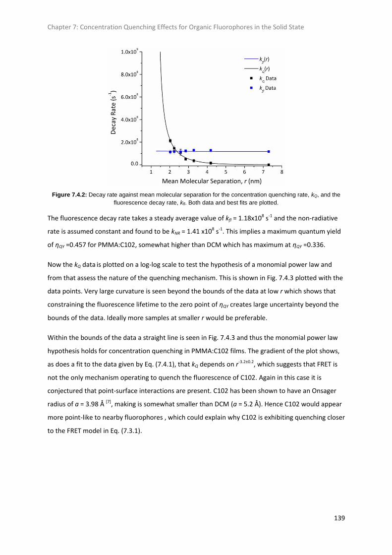
Chapter 7: Concentration Quenching Effects for Organic Fluorophores in the Solid State
139
Figure 7.4.2: Decay rate against mean molecular separation for the concentration quenching rate, kQ, and the
fluorescence decay rate, kfl. Both data and best fits are plotted.
The fluorescence decay rate takes a steady average value of kfl = 1.18x10⁸ s-1 and the non-radiative
rate is assumed constant and found to be kNR = 1.41 x10⁸ s-1. This implies a maximum quantum yield
of ηQY =0.457 for PMMA:C102, somewhat higher than DCM which has maximum at ηQY =0.336.
Now the kQ data is plotted on a log-log scale to test the hypothesis of a monomial power law and
from that assess the nature of the quenching mechanism. This is shown in Fig. 7.4.3 plotted with the
data points. Very large curvature is seen beyond the bounds of the data at low r which shows that
constraining the fluorescence lifetime to the zero point of ηQY creates large uncertainty beyond the
bounds of the data. Ideally more samples at smaller r would be preferable.
Within the bounds of the data a straight line is seen in Fig. 7.4.3 and thus the monomial power law
hypothesis holds for concentration quenching in PMMA:C102 films. The gradient of the plot shows,
as does a fit to the data given by Eq. (7.4.1), that kQ depends on r-3.2±0.2, which suggests that FRET is
not the only mechanism operating to quench the fluorescence of C102. Again in this case it is
conjectured that point-surface interactions are present. C102 has been shown to have an Onsager
radius of a = 3.98 Å [7], making is somewhat smaller than DCM (a = 5.2 Å). Hence C102 would appear
more point-like to nearby fluorophores , which could explain why C102 is exhibiting quenching closer
to the FRET model in Eq. (7.3.1).
Chapter 7: Concentration Quenching Effects for Organic Fluorophores in the Solid State
140
Figure 7.4.3: A log-log plot of concentration quenching rate against mean molecular separation is plotted here for
C102. Both the best fit function of kQ(r) (red line) and data points are shown.
Comparing Eqs. (7.3.5) and (7.4.1) the numerator takes a similar value. For these equations to
balance dimensionally the numerators must have rather odd units; in the case of Eq. (7.4.1) this is
nm4.18s-1. This is attributed to this monomial expression being the empirical equivalent of more than
one quenching mechanism. The powers of r in these equations represent the gradients of the linear
fits to the data in Figs. 7.3.3 and 7.4.3 and the numerators are the values kQ would have at r = 1 nm,
though as has been seen the quantum yield falls to zero before this point anyway.
C102 shows a stronger dependence on r than DCM but this also means that the range of the
quenching process is longer for DCM. The non-radiative rate for DCM is considerably higher at
2.84x10⁸ s-1 compared to 1.41x10⁸ s-1 for C102 whereas DCM has a faster fluorescence rate at
1.44x10⁸ s-1 compared to 1.18x10⁸ s-1. These values give maximum quantum yields of 0.336 and
0.457 for DCM and C102 respectively. This seems to be correct but quantum yield measurements of
very low concentrations for DCM, shown in Fig. 7.2.1, indicate this is not quite accurate since DCM
was measured to have ηQY = 0.45 ± 0.05 at Cdye = 1x10⁻⁴ M (r = 25.44) in PMMA. For a truer analysis
samples over a greater range of fluorophore concentrations should have been measured with
correspondent pairs of quantum yield and fluorescence lifetime data.
Chapter 7: Concentration Quenching Effects for Organic Fluorophores in the Solid State
141
7.5 Conclusion
The results of this chapter have shown that concentration quenching is a significant effect for all
fluorophores and the host material itself has an important role to play in providing a stable, inert
environment. DCM class fluorophores are found to be much less efficient than perylene based ones
and it is apparent that different fluorophores exhibit differing quantum yield dependence on
concentration. This suggests a range of quenching processes are being observed in many of the
organic fluorophores studied.
The quenching process was seen to likely be the result of a combination of quenching mechanisms
for two of the fluorophores studied, DCM and C102, based on the dependence on mean molecular
separation, r, observed. The form of the dependence was seen to be of a monomial power law in
terms of r to the power of -2.9±0.2 and -3.2±0.2 for DCM and C102, respectively. These values tell us
the combined effect of all quenching processes is of longer range than point-like dipole-dipole
interactions, proportional to r-6. Point-surface and surface-surface interactions may be responsible
for this deviation. If aggregates of fluorophores form between host polymer fibres then the
proximity may lead to surface-like dipole distributions. electronic interaction with the host polymer
may also be responsible. The result of a longer range effect is for the quantum yield to fall into
decline at longer r, which is undesirable in LSC devices as lower concentrations and thicker devices
will be necessary.
Chapter 7: Concentration Quenching Effects for Organic Fluorophores in the Solid State
142
7.6 References
[1] Y. Kawamura, J. Brooks, J. J. Brown, H. Sasabe and C. Adachi, Intermolecular Interaction and a
Concentration-Quenching Mechanism of Phosphorescent Ir(III) Complexes in a Solid Film, Phys. Rev.
Lett. 96, 017404 (2006)
[2] J. Cabanillas-Gonzalez, A. M. Fox, J. Hill and D. D. C. Bradley, Model for Energy Transfer in
Polymer/Dye Blends Based on Point-Surface Dipole Interaction, Chem. Mater. 16, 4705-4710 (2004)
[3] J. Hill, S. Y. Heriot, O. Worsfold, T. H. Richardson, A. M. Fox and D. D. C. Bradley, Dynamics of
Förster transfer in polyfluorene-based polymer blends and Langmuir-Blodgett nanostructures, Synth.
Met. 139, 787-790 (2003)
[4] Rabih O. Al-Kaysi et. al., The Photophysical Properties of Chromophores at High (100mM and
above) Concentrations in Polymers and as Neat Solids, Phys. Chem. Chem. Phys. 8, 3453-3459 (2006)
[5] S. A. Bagnich and V. N. Knyukshto, Quenching of Fluorescence of Conjugated Poly(p-Pheylene)
Polymers by Benzil and Dimethylaminobenzil Molecules, J. Appl. Spec. 73, 6 (2006)
[6] F. Fennel and S. Lochbrunner, Long distance energy transfer in a polymer matrix doped with a
perylene dye, Phys. Chem. Chem. Phys. 13, 3527-3533 (2011)
[7] J. Y. Choi, E. J. Park, S. H. Chang and T. J. Kang, Solvent Effects on the Solvatochromism of 7-
Aminocoumarin Derivatives in Neat and Binary Solvent Mixtures: Correlation of the Electronic
Transition Energies with the Solvent Polarity Parameters, Bull. Korean Chem. Soc. 30, 7, 1452-1458
(2009)
Chapter 8: Spectral Based Models and Implications for LSC Devices
143
Chapter 8
Spectral Based Models and Implications for LSC Devices
8.1 Introduction
In this final results chapter many of the preceding results are brought together to build a model in
order to try and answer some fundamental questions about LSC technology and the performances
that can be achieved. What kind of optical concentrations and performances can one expect from an
LSC with the materials studied in this thesis? What are the optimal LSC properties to maximise
output power? What kind of cost efficiencies can be achieved? How will solvation improve LSC
performance?
To answer these kinds of questions on performance we turn back to the definition of optical
concentration and the various associated efficiencies, which were laid out in chapter 2.2 and 2.3.
The optical concentration, Copt, is given in Eq. (2.3.2) as the product of the optical efficiency, ηopt, and
the geometric concentration, G, which are given by Eqs. (2.2.15) and (2.3.1) respectively. By
assuming suitable physical ranges for the different efficiency parameters, and the geometry of the
LSC, various scenarios can be formed in a spectral based modelling approach. In section 8.2 a
hypothetical ideal LSC is realised to calculate an upper limit of optical concentration.
The choice of model chosen for this work is different from those employed in literature [1] due to
time constraints on this thesis and hence a requirement for ease of design. Typically either
thermodynamic [2-4] or ray-tracing approaches [5-8] are used which are more accurate and therefore
deserve discussion in some detail. Both of these modelling techniques require considerably more
computational power than the spectral based model developed here, which stands as a clear
advantage of the current work. However the accuracy and hence applicability to experiment is more
limited in this case, for reasons to be discussed.
Thermodynamic modelling uses detailed balance arguments to relate the absorption and emission in
terms of flux in 3D, allowing the photon chemical potential as a function of position to be
determined. Detailed analytical expressions can be derived from this approach allowing accurate
predictions of LSC device irradiance and power output. Such models can also be expanded using
boundary conditions from experiment, for example when modelling how cholesteric coatings can be
used as wavelength selective mirrors [4]. These models still make idealised assumptions about device

Chapter 8: Spectral Based Models and Implications for LSC Devices
144
properties but are very instructive in optimising LSC performance. Compared to ray-tracing the
thermodynamic approach requires less input data and is computationally less expensive.
3D ray-tracing models work by tracking individual photon paths through the device, the standard
approach being to use a statistically averaged absorption process to reduce computation time [5, 6].
An extension to this in more recent ray-tracing models is to introduce the absorption and emission
of the fluorophore [7, 8]. Ray-tracing provides more flexibility than other modelling approaches as it
can be adapted to include multiple dyes, different LSC geometries and the modelling of thin film
device structures. It has been shown to have a similar accuracy in prediction to the thermodynamic
approach [1] and is fast becoming the dominant method.
The main advantages of the spectral modelling approach used here is in its analytical simplicity and
low computational requirements. It still requires a significant amount of input data, discussed next,
which include all sorts of properties about the different components in the concentration and
conversion process, from sun to LSC to solar cell. The model exhibited here has not been developed
to treat for more complex geometries and device architectures but could in principle do so with the
right inputs and boundary conditions. Therefore it has the potential to be as flexible as ray-tracing
approaches. Considering that it provides poorer accuracy with respect to experiment it is clear as to
why the spectral modelling method not really used, particularly considering the wide availability of
computational power.
Section 8.3 discusses the methods for predicting LSC performance by a detailed spectral analysis and
methods for optimisation. Performance is characterised by the LSC output irradiance, SLSC(λ), the
resultant power generated by an attached solar cell, Pout, and hence the LSC power conversion
efficiency, ηLSC. These quantities are determined by knowing key inputs for the model which are; the
solar irradiance spectrum, Ssun(λ), host refractive index, n2, fluorophore extinction spectrum, ε(λ),
fluorophore quantum yield as a function of concentration, ηQY(Cdye), normalised fluorophore
emission spectrum, SN(λ), and the solar cell power conversion efficiency spectrum, ηPCE(λ). Other
efficiencies on which the optical efficiency of Eq. (2.2.15) depends are calculated through the
spectral model or otherwise given reasonable assumed values from literature. LSC models are
constrained to the square-planar geometry with a range of dimensions and geometric
concentrations, G, explored.
Performance of the modelled LSC structures is also characterised by the £/W cost efficiency, which is
calculated on the basis of the LSC volume and area of solar cells using reasoned cost values
discussed in section 8.4.
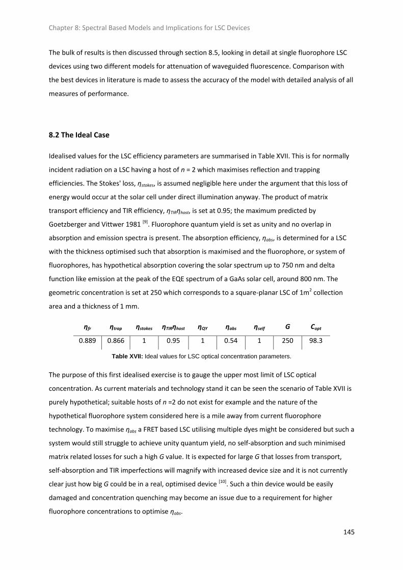
Chapter 8: Spectral Based Models and Implications for LSC Devices
145
The bulk of results is then discussed through section 8.5, looking in detail at single fluorophore LSC
devices using two different models for attenuation of waveguided fluorescence. Comparison with
the best devices in literature is made to assess the accuracy of the model with detailed analysis of all
measures of performance.
8.2 The Ideal Case
Idealised values for the LSC efficiency parameters are summarised in Table XVII. This is for normally
incident radiation on a LSC having a host of n = 2 which maximises reflection and trapping
efficiencies. The Stokes' loss, ηstokes, is assumed negligible here under the argument that this loss of
energy would occur at the solar cell under direct illumination anyway. The product of matrix
transport efficiency and TIR efficiency, ηTIRηhost, is set at 0.95; the maximum predicted by
Goetzberger and Vittwer 1981 [9]. Fluorophore quantum yield is set as unity and no overlap in
absorption and emission spectra is present. The absorption efficiency, ηabs, is determined for a LSC
with the thickness optimised such that absorption is maximised and the fluorophore, or system of
fluorophores, has hypothetical absorption covering the solar spectrum up to 750 nm and delta
function like emission at the peak of the EQE spectrum of a GaAs solar cell, around 800 nm. The
geometric concentration is set at 250 which corresponds to a square-planar LSC of 1m2 collection
area and a thickness of 1 mm.
ηfr ηtrap ηstokes ηTIRηhost ηQY ηabs ηself G Copt
0.889 0.866 1 0.95 1 0.54 1 250 98.3
Table XVII: Ideal values for LSC optical concentration parameters.
The purpose of this first idealised exercise is to gauge the upper most limit of LSC optical
concentration. As current materials and technology stand it can be seen the scenario of Table XVII is
purely hypothetical; suitable hosts of n =2 do not exist for example and the nature of the
hypothetical fluorophore system considered here is a mile away from current fluorophore
technology. To maximise ηabs a FRET based LSC utilising multiple dyes might be considered but such a
system would still struggle to achieve unity quantum yield, no self-absorption and such minimised
matrix related losses for such a high G value. It is expected for large G that losses from transport,
self-absorption and TIR imperfections will magnify with increased device size and it is not currently
clear just how big G could be in a real, optimised device [10]. Such a thin device would be easily
damaged and concentration quenching may become an issue due to a requirement for higher
fluorophore concentrations to optimise ηabs.

Chapter 8: Spectral Based Models and Implications for LSC Devices
146
8.3 Predicting LSC Power Output Using a Spectral Based Approach
Some more realistic scenarios shall now be considered in greater detail using methods developed in
chapter 2.2 and 2.5 to make estimates of the relevant parameters. The relevant parameters are as in
Table XVII on the previous page; Copt, G, ηopt, ηfr, ηtrap, ηstokes, ηTIR, ηhost, ηQY, ηabs and ηself. The total
internal reflection efficiency will take the best value predicted, ηTIR = 0.99, and ηstokes = 0.75 [9] as
discussed in chapter 2, page. For these models square-planar concentrators are considered for
various G and mean path length, <r>, which impacts on self-absorption. Cylindrical LSC devices are
only worth considering for bi-layer structures due to the way trapping efficiency increases with
distance from the centre of the cylinder [5, 11]. Because of this, and the complexity of the
mathematics, bi-layer cylindrical devices cannot be considered here but have elsewhere in ray-
tracing models [5, 8] and for PR doped fibre LSC devices [12].
The aim is to find Copt but also, using Eqs. (2.2.10), (2.2.13) and (2.2.15), to determine the irradiant
intensity of light arriving at the solar cell. Then using external quantum efficiency spectra , ηEQE(λ),
for various solar cells digitised from graphical data with known power conversion efficiencies [13-15],
the power conversion efficiency spectra were determined as discussed in chapter 2.5 using Eq.
(2.5.3). Also note that now, because of Eq. (2.2.13), the optical efficiency, and therefore Copt, is a
function of wavelength due to the self-absorption process. Matrix related losses would also depend
on wavelength but are quantified more simply in this exercise by the host attenuation at 550 nm.
Since only PMMA is considered an attenuation of 3.5x10⁻⁴ cm-1 is adopted for calculating ηhost
throughout the models presented here.
First is to think about the fluorophore to be used; several basic single dye designs will be considered
using DCJTB, PR and Perylene. Other fluorophores were considered but PR shows the best
absorption properties and DCJTB offers the chance to exhibit the solvation enhancement, explored
previously in chapter 5. Perylene is a very high quantum yield blue-green emitter and is therefore a
good choice for the upper plate of a tandem LSC. These fluorophores have properties summarised in
Table II on page 42, chapter 2.4, including extinction coefficients.
With these fluorophores in mind it is important to choose the optimum solar cell for absorbing the
emission wavelengths. Fig. 8.3.1 shows a selection of solar cell ηPCE(λ) spectra with the peak
wavelengths of each dye shown. Clearly the GaAs solar cell will the best choice for each fluorophore
followed by CIGS cells for DCJTB and PR and c:Si cells for Perylene.
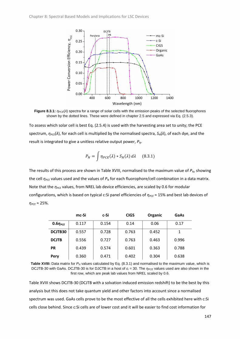
Chapter 8: Spectral Based Models and Implications for LSC Devices
147
Figure 8.3.1: ηPCE(λ) spectra for a range of solar cells with the emission peaks of the selected fluorophores
shown by the dotted lines. These were defined in chapter 2.5 and expressed via Eq. (2.5.3).
To assess which solar cell is best Eq. (2.5.4) is used with the harvesting area set to unity; the PCE
spectrum, ηPCE(λ), for each cell is multiplied by the normalised spectra, SN(λ), of each dye, and the
result is integrated to give a unitless relative output power, PN.
The results of this process are shown in Table XVIII, normalised to the maximum value of PN, showing
the cell ηPCE values used and the values of PN for each fluorophore/cell combination in a data matrix.
Note that the ηPCE values, from NREL lab device efficiencies, are scaled by 0.6 for modular
configurations, which is based on typical c:Si panel efficiencies of ηPCE ≈ 15% and best lab devices of
ηPCE ≈ 25%.
mc-Si c-Si CIGS Organic GaAs
0.6ηPCE 0.117 0.154 0.14 0.06 0.17
DCJTB30 0.557 0.728 0.763 0.452 1
DCJTB 0.556 0.727 0.763 0.463 0.996
PR 0.439 0.574 0.601 0.363 0.788
Pery 0.360 0.471 0.402 0.304 0.638
Table XVIII: Data matrix for PN values calculated by Eq. (8.3.1) and normalised to the maximum value, which is
DCJTB-30 with GaAs. DCJTB-30 is for DJCTB in a host of εr = 30. The ηPCE values used are also shown in the
first row, which are peak lab values from NREL scaled by 0.6.
Table XVIII shows DCJTB-30 (DCJTB with a solvation induced emission redshift) to be the best by this
analysis but this does not take quantum yield and other factors into account since a normalised
spectrum was used. GaAs cells prove to be the most effective of all the cells exhibited here with c:Si
cells close behind. Since c:Si cells are of lower cost and it will be easier to find cost information for

Chapter 8: Spectral Based Models and Implications for LSC Devices
148
them their power conversion spectrum will be used here for the most part. Some models with GaAs
cells are explored since the best devices in literature have used them. It seems reasonable to assume
the very best technology for an LSC since the point is to reduce the area of the solar cells required
and PCE gains are to be had by removing the need for large area modular devices where losses are
greater.
The next step in the recipe is to determine the reflection efficiency, ηfr, and the trapping efficiency,
ηtrap. These depend on the host refractive index, n, and, for ηfr, on the angle of incidence of solar
irradiance. The irradiance entering the device is given by the product of the solar irradiance
spectrum, Ssun(λ), and ηfr, to give the transmitted irradiance, T(λ). The chosen solar spectrum is the
AM1.5 global irradiance spectrum from NREL [16].
The average absorption path length for light, l, is then given by Eq. (8.3.2) through Snell's law.
Where W is the LSC thickness and the factor of 2 comes from the back reflector giving rise to two
passes through the device. A device designed to absorb diffuse light may therefore benefit from
being thinner because the absorption length is on average greater, since diffuse light comes from
many angles, and one could increase G to improve the diffuse yield in this way. At θi = 42.75° for
PMMA we find l = 1.123W, which is a significant increase in absorption length compared to l = W for
normal incidence.
Using the absorption length and the extinction coefficients of the fluorophores allows the absorbed
intensity, S0(λ), to be determined using Eq. (2.2.5) in a similar way to that done in chapter 6.4, but
with the irradiance input T(λ) = ηfrSsun(λ). Then the absorption efficiency, ηabs, is easily found by
comparing the absorbed intensity to the total incident intensity. From S0(λ), measured ηQY values
and using Eq. (2.2.10) the quantum yield corrected equivalent intensity spectrum, S1(λ), is
determined. This is the irradiance spectrum of the first order emission to be propagated through the
device.
For propagation of light through waveguide modes we must consider the self-absorption, host
attenuation and TIR processes. As discussed in chapter 2, page 18, the TIR efficiency is expected to
have a near unity value and is set at ηTIR = 0.99. The host attenuation is modelled using the
absorption coefficient for pure PMMA measured at 550 nm, which is around αh ≈ 3.5x10⁻⁴ cm-1. The
Eq. 2.2.6 in chapter 2 then gives the host efficiency as . Lastly then ηself is

Chapter 8: Spectral Based Models and Implications for LSC Devices
149
described by Eq. (2.2.13) and the mean path length of waveguide modes in square planar
concentrators is described by Eq. (2.2.14). In Eq. (2.2.13) the self-absorbed irradiance spectrum is
seen as , which is set as the new S0(λ) in Eq. (2.2.10) in an iterative process
that generates an irradiance spectrum for each order of emission. The actual emission from a given
order that reaches the solar cell is thus taken to be ηTIRηstokesSp(λ) for the pth
order where ηTIRηstokes = 0.7425. Additionally the final LSC irradiance output, SLSC(λ), must be
corrected for the geometric ratio, G, to take account of the concentration effect. Hence the
combined LSC irradiance output for all p orders is given by the sum in Eq. (8.3.3).
Eq. (8.3.3) generates a spectrum which has been corrected for all losses through the LSC as faithfully
as the available data allows. Strong confidence should be reasonable on both ηQY and ηself given
available spectral and quantum yield information, though local variance in concentration will affect
these values. The lack of information for ηhost, which is likely to have some wavelength dependence,
will result in some deviation in spectral shape and power density distribution from reality. An
example set of LSC spectra calculated using these equations is shown in Fig. 8.3.2 for PR with G =
31.25 and <r> = 26.7 cm.
Figure 8.3.2: Plotted here for the fluorophore PR is; the absorbed irradiance spectrum, S0(λ), the emission
irradiance spectrum for each order of emission after losses, S1(λ), S2(λ), and S3(λ), and their sum, SLSC(λ). LSC
dimensions are W = 4 mm, L = 50 m, hence G = 31.25 and <r> = 26.7 cm. The correction GηTIRηhostηstokes = 22.99
is applied to emission and LSC output spectra, which gives a physical result for the concentrated irradiance,
whereas the absorbed irradiance is scaled by the same factor for illustration.
As Figure 8.3.2 shows that the absorbed intensity is much smaller than the concentrated irradiance
the LSC is outputting to the solar cells. This is due to the geometric concentration, quantified
Chapter 8: Spectral Based Models and Implications for LSC Devices
150
through G. The total irradiance output for the case in Fig. 8.3.2 is equivalent to an optical efficiency
of ηopt ≈ 6% and an optical concentration of Copt = 1.87 suns. Self-absorption is evident but after the
average path length of 26.7 cm there is still some overlap and self-absorption is not exhausted.
With the result in Eq. (8.3.3) an equation similar to Eq. (8.3.1) can now be written to calculate the
output power of the LSC. Replacing Ssun(λ) in Eq. (2.5.4) with SLSC(λ) and then multiplying through by
the area of solar cell, Ahar, gives the power collected, as in Eq. (8.3.4). Note also the power correction
factor, β, which corrects for change in solar cell efficiency with light intensity, as explained in chapter
2, page 48.
As was done in chapter 5 on the solvation enhancement of ηself, the optical efficiency, ηopt, can be
calculated up to the third generation using Eq. (2.2.15), at which point further orders of self-
absorption and emission are considered negligible.
A back reflector, with reflectivity = 0.97, will generally be used to maximise absorption which
introduces a factor of two in absorption path length equations. It also introduces a small
contribution to the LSC output from cone light from all escape cones facing the back reflector,
leading to a modified Eq. (8.3.3) for the output irradiance spectrum. ECL transfer gains of this sort
can be quite large, up to several percent of the total output irradiance with a strong dependence on
dye concentration. The LSC plate emits total S1(λ)/ηtrap for each emission order, determined as
discussed above, and of this a fraction (1 - ηtrap) escapes via ECL, so the irradiance spectrum leaving
via the escape cones, SECL(λ), is given by Eq. (8.3.5).
Note that the ECL irradiance doesn't suffer from a ηTIR; this is because TIR is irrelevant since escape
cone light does not internally reflect. Also note the irradiance for the pth order is divided by ηtrap due
to the definition of Sp(λ) from Eq. (2.2.10). Only one of the two escape cones is directed onto the
back reflector and so the ECL irradiance that is reflected is given by half of Eq. (8.3.5). The angle at
which this occurs is again done on average. For PMMA with n = 1.492 gives critical angle θc = 42.09°
and hence θECL = 21.05°. By replacing θi with θECL in Eq. (8.3.2) the mean absorption path length for
this contribution is determined and hence the self-absorbed irradiance spectrum can be found. Note
that on average light is emitted at height W/2 in the z plane, so the total z distance is 3W/2 for back
Chapter 8: Spectral Based Models and Implications for LSC Devices
151
reflected irradiance. As before the self-absorbed irradiance is translated to an emission irradiance
via Eq. (2.2.10) and this contribution propagated to the LSC edge.
We also need to consider is what values of geometric ratio, G, to use and there are two ways to do
this. First is to optimise G for each dye by the absorption path length of the incident irradiance
(hence the thickness of the LSC plate) in light of the extinction coefficients. DCJTB has greater
extinction than perylene or PR and hence will benefit by reduced thickness and enhanced G. The
other way is to use the same values of G but tune the fluorophore concentration, hence quantum
yield and normalised emission spectrum, of the fluorophores to achieve optimised absorption
efficiency. Here the second approach is preferred as comparing LSC devices of different G values is
unnecessarily complicated.
This is done with the fluorophores detailed above whose optimised concentrations are dictated by
both the need to maximise absorption of incident light and reduce loss across the LSC. The size of
the LSC is critical in this because of self-absorption and host attenuation. Thicker plates achieve peak
output at lower concentrations because they require less dye to maximise absorption of sunlight.
The energy density coming out of the LSC is lower for thicker plates, due to having a lower G, but the
amount of power generated also depends on the area of solar cells, so thicker plates may still
generate more power.
The peak of irradiance output occurs for Cdye between 10-4 M and 10-3 M, depending on which
fluorophore we look at and the LSC plate dimensions. Optimised quantum yield/fluorophore
concentration, self-absorption and absorption of incident radiation are contained within this
characterisation. For the fluorophore concentrations both PR and DCJTB use Cdye = 10-4 M and
perylene uses Cdye = 5x10⁻⁴ M.
Everything that has been developed above leads to determining the optical concentration, Copt, the
LSC output spectrum, SLSC(λ), and from this the power generated by the cell, Pout.. The ratio of the
integral of SLSC(λ) to that of the solar irradiance spectrum, Ssun(λ), should be equal to Copt calculated
by Eqs. (2.2.15) and (2.3.2), since they are determined with the same inputs. One can now also
calculate the LSC power conversion efficiency, ηLSC, which is given by the ratio of power in to power
out as in Eq. (8.3.6).
Where Pin is the integral of solar irradiance spectrum times by collection area, Acol, and Pout is given
by Eq. (8.3.4). As discussed in chapter 2.6 the two best state of the art LSC devices give ηLSC = 7.1% [17]
Chapter 8: Spectral Based Models and Implications for LSC Devices
152
and ηLSC = 6.7% [18] for devices of dimensions 5 x 5 x 0.5 cm (G = 2.5) and a two stack of 2 x 2 x 0.3 cm
(G = 5/3), respectively. Both of these used two dye systems and will make interesting comparison for
some of the models produced here. These LSC devices and others in literature are seen in Table VI,
chapter 2.6, page 50.
8.4 Estimating the Cost Efficiency of a LSC Device
The last thing that can be estimated is the cost per unit power delivered by the modelled device
structures. This has been done in detail alongside LSC device optimisation through ray-tracing
simulations [19]. In that work the performance is characterised through three measures; the cost per
unit area, power output per unit area and their ratio The LSC structure will have a cost per unit
volume for the host and dye materials. The solar cell will have a cost per unit area; production costs
are included by considering the cost of typical c:Si panels available online. These costs are
determined for the given LSC structure of volume, VLSC, dye concentration, Cdye (in mol m-3), and solar
cell area, Ahar. By summing the costs and dividing the result by the power estimated by the model we
arrive at an estimate of the cost per unit power delivered, (£/W)conc, with the target to achieve
< 0.61 £/W (or < 1 $/W). This is given by Eq. (8.4.1).
By canvassing c:Si solar panels online that are available to end users, typically with cost efficiency
around 1$/W, one arrives at a panel cost per unit area of (£c:Si/m2) ≈ £ 120 m-2. This number includes
balance of system (BOS) costs in production and transport which will suffice for approximating the
BOS for our hypothetical LSC devices.
The fluorophores PR, DCJTB and perylene can be found available at various laser accessory retailers
but the profit mark-up and poor economies of scale at such vendors make the prices uneconomic.
For example Photonic Solutions Ltd. sells PR under Exciton trade name Exalite 613 at £140 per g. Not
a great deal; compare this to Rhodamine 6G, a fluorophore often used in LSC research and in other
scientific pursuits, which comes at £15 per g from the same source. Clearly economies of scale allow
for reduction of price by an order of magnitude and will be taken as 2% [20] of the prices found from
sources such as Photonics Solutions Ltd. These are taken to be £1.8 g-1, £2.8 g-1 and £1 g-1 for DCJTB,
PR and perylene respectively. With the cost per gram known the (£dye/mol) cost can be found from
Chapter 8: Spectral Based Models and Implications for LSC Devices
153
the molecular weights, which are 453.63 g mol-1, 963.956 g mol-1 and 252.32 g mol-1 for DCJTB, PR
and perylene, respectively. Now (£dye/mol) ≈ £ 820 mol-1, £2700 mol-1 and £250 mol-1 for DCJTB, PR
and perylene respectively. PR is significantly more expensive by this analysis which will offset gains in
power due to its better performance.
The final cost to approximate is the cost of the host material. PMMA is produced on larges scales by
various techniques. Companies such as Shenzhen Xintao Acrylic Co. Ltd. use extrusion to create
highly uniform sheets of such thermoplastics, which may be a viable large scale production method
for LSC devices. Typical costs are at around £2 per kg of material extruded and 50% should be added
to account for complexities in the process introduced by the requirements of a LSC. So at £3 per kg
with the density of PMMA at ρPMMA = 1180 kg m-3 we find a cost of (£host/m3) ≈ £3500 m-3.
For DCJTB with the solvation enhancement some extra cost must be factored in for some high
permittivity material to induce the effect. TiO2 nanoparticles can be bought, silane coated for
dissolving in solution, at around £360 per kg from companies like SkySpring Nanomaterials, Inc. TiO2
has a relative permittivity around 100 and hence around 28 wt% of TiO2 nanoparticles in PMMA is
required to achieve εr = 30, which is an impractically high concentration. If it were SrBaTiO3, a more
expensive titanate, only 2 wt% would be required as it has a permittivity of 1250. Assuming ten
times the cost for SrBaTiO3, £3600 per kg, then for every m3 of host 23.6 kg of nanoparticles are
needed, hence (£SrBaTiO3/m3) ≈ £85000 m-3. This cost is added in with host costs and greatly increases
the cost of the concentrator.
All of the cost considerations here are based on reasonable approximations but are still quite
arguable. They are meant to give a ballpark cost efficiency to consider, approached with the caution
of appreciation of the large uncertainties involved.
8.5 Spectral Analysis for a Single Fluorophore LSC Devices
In this first results section single fluorophore plates are considered for perylene, PR, DCJTB and
DCJTB-30, which is for DCJTB influenced by the solvation effect with host permittivity at εr = 30. For
each fluorophore the model requires the quantum yield, ηQY(Cdye), extinction coefficients, ε(λ), and
the normalised emission spectrum, SN(λ). The latter two are seen in chapter 2.4 and the fluorophore
quantum yields are determined for a given concentration from fits to the data in Fig. 7.2.1.
Other inputs to model are; the AM1.5 global solar irradiance spectrum, Ssun(λ), which is incident at
normal incidence, θi = 0°, on a host of n = 1.492, that of PMMA. This sets the reflection and trapping
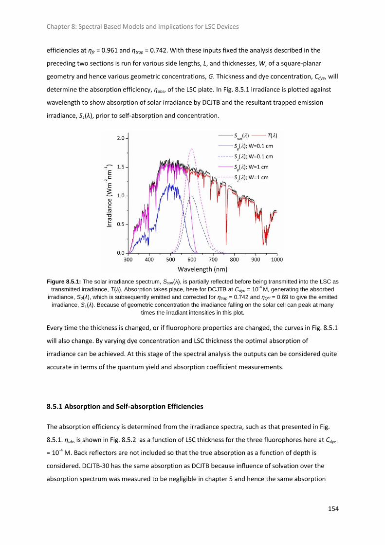
Chapter 8: Spectral Based Models and Implications for LSC Devices
154
efficiencies at ηfr = 0.961 and ηtrap = 0.742. With these inputs fixed the analysis described in the
preceding two sections is run for various side lengths, L, and thicknesses, W, of a square-planar
geometry and hence various geometric concentrations, G. Thickness and dye concentration, Cdye, will
determine the absorption efficiency, ηabs, of the LSC plate. In Fig. 8.5.1 irradiance is plotted against
wavelength to show absorption of solar irradiance by DCJTB and the resultant trapped emission
irradiance, S1(λ), prior to self-absorption and concentration.
Figure 8.5.1: The solar irradiance spectrum, Ssun(λ), is partially reflected before being transmitted into the LSC as
transmitted irradiance, T(λ). Absorption takes place, here for DCJTB at Cdye = 10-4
M, generating the absorbed
irradiance, S0(λ), which is subsequently emitted and corrected for ηtrap = 0.742 and ηQY = 0.69 to give the emitted
irradiance, S1(λ). Because of geometric concentration the irradiance falling on the solar cell can peak at many
times the irradiant intensities in this plot.
Every time the thickness is changed, or if fluorophore properties are changed, the curves in Fig. 8.5.1
will also change. By varying dye concentration and LSC thickness the optimal absorption of
irradiance can be achieved. At this stage of the spectral analysis the outputs can be considered quite
accurate in terms of the quantum yield and absorption coefficient measurements.
8.5.1 Absorption and Self-absorption Efficiencies
The absorption efficiency is determined from the irradiance spectra, such as that presented in Fig.
8.5.1. ηabs is shown in Fig. 8.5.2 as a function of LSC thickness for the three fluorophores here at Cdye
= 10-4 M. Back reflectors are not included so that the true absorption as a function of depth is
considered. DCJTB-30 has the same absorption as DCJTB because influence of solvation over the
absorption spectrum was measured to be negligible in chapter 5 and hence the same absorption
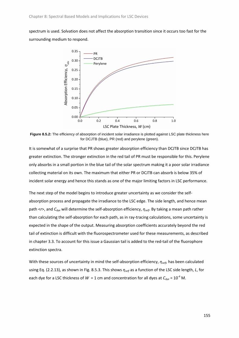
Chapter 8: Spectral Based Models and Implications for LSC Devices
155
spectrum is used. Solvation does not affect the absorption transition since it occurs too fast for the
surrounding medium to respond.
Figure 8.5.2: The efficiency of absorption of incident solar irradiance is plotted against LSC plate thickness here
for DCJTB (blue), PR (red) and perylene (green).
It is somewhat of a surprise that PR shows greater absorption efficiency than DCJTB since DCJTB has
greater extinction. The stronger extinction in the red tail of PR must be responsible for this. Perylene
only absorbs in a small portion in the blue tail of the solar spectrum making it a poor solar irradiance
collecting material on its own. The maximum that either PR or DCJTB can absorb is below 35% of
incident solar energy and hence this stands as one of the major limiting factors in LSC performance.
The next step of the model begins to introduce greater uncertainty as we consider the self-
absorption process and propagate the irradiance to the LSC edge. The side length, and hence mean
path <r>, and Cdye will determine the self-absorption efficiency, ηself. By taking a mean path rather
than calculating the self-absorption for each path, as in ray-tracing calculations, some uncertainty is
expected in the shape of the output. Measuring absorption coefficients accurately beyond the red
tail of extinction is difficult with the fluorospectrometer used for these measurements, as described
in chapter 3.3. To account for this issue a Gaussian tail is added to the red-tail of the fluorophore
extinction spectra.
With these sources of uncertainty in mind the self-absorption efficiency, ηself, has been calculated
using Eq. (2.2.13), as shown in Fig. 8.5.3. This shows ηself as a function of the LSC side length, L, for
each dye for a LSC thickness of W = 1 cm and concentration for all dyes at Cdye = 10-4 M.
Chapter 8: Spectral Based Models and Implications for LSC Devices
156
Figure 8.5.3: Self-absorption efficiency against LSC side length for LSC devices of W = 1cm. Each of DCJTB-30
(black), DCJTB (blue), PR (red) and perylene (green) are shown.
Fig. 8.5.3 gives insight into the workings of the model. DCJTB-30 shows much higher ηself values than
the other fluorophores thanks to solvation induced redshift of emission. The models show that the
self-absorption efficiency reaches a steady value after a certain side length of LSC, which is due to
total absorption of the all irradiance in the extinction region. To ensure optimal absorption of solar
irradiance a perylene based LSC plate must be thicker to achieve lower fluorophore concentrations
and therefore longer lengths. This is an important point if a tandem LSC were considered; it is
desirable to match the side lengths of the stack layers but some layers may find optimum ηLSC for
different thicknesses.
The model shows a sharp dependence on side length below 2.5m, particularly for lower LSC lengths
which indicate that as the LSC side length tends to 0 the self-absorption efficiency will tend to unity.
However, such sizes are not particularly practical in terms of power generation due to low geometric
ratios and sub-solar irradiant output, which means the c:Si solar cell will not be operating at
optimum efficiency.
8.5.2 Optical Concentration
With the absorption and self-absorption efficiencies determined it is now possible to determine both
the optical concentration, Copt, and the LSC output irradiance, SLSC(λ), as outlined in section 8.2. As
stated in that section the ratio of the integral of SLSC(λ) to that of the input solar irradiance, Ssun(λ),
should be equal to Copt. This will not be true when using Eq. (2.2.15) for the optical efficiency, ηopt,
because this does not account for addition of escape cone gains due to back reflection. Since back
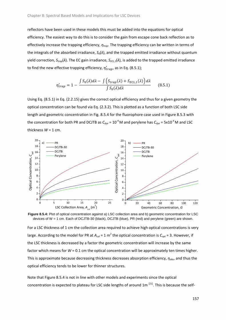
Chapter 8: Spectral Based Models and Implications for LSC Devices
157
reflectors have been used in these models this must be added into the equations for optical
efficiency. The easiest way to do this is to consider the gain from escape cone back reflection as to
effectively increase the trapping efficiency, ηtrap. The trapping efficiency can be written in terms of
the integrals of the absorbed irradiance, S0(λ), and the trapped emitted irradiance without quantum
yield correction, Strap(λ). The EC gain irradiance, SECL,1(λ), is added to the trapped emitted irradiance
to find the new effective trapping efficiency, , as in Eq. (8.5.1);
Using Eq. (8.5.1) in Eq. (2.2.15) gives the correct optical efficiency and thus for a given geometry the
optical concentration can be found via Eq. (2.3.2). This is plotted as a function of both LSC side
length and geometric concentration in Fig. 8.5.4 for the fluorophore case used in Figure 8.5.3 with
the concentration for both PR and DCJTB as Cdye = 10-4 M and perylene has Cdye = 5x10⁻⁴ M and LSC
thickness W = 1 cm.
Figure 8.5.4: Plot of optical concentration against a) LSC collection area and b) geometric concentration for LSC
devices of W = 1 cm. Each of DCJTB-30 (black), DCJTB (blue), PR (red) and perylene (green) are shown.
For a LSC thickness of 1 cm the collection area required to achieve high optical concentrations is very
large. According to the model for PR at Acol = 1 m2 the optical concentration is Copt ≈ 3. However, if
the LSC thickness is decreased by a factor the geometric concentration will increase by the same
factor which means for W = 0.1 cm the optical concentration will be approximately ten times higher.
This is approximate because decreasing thickness decreases absorption efficiency, ηabs, and thus the
optical efficiency tends to be lower for thinner structures.
Note that Figure 8.5.4 is not in line with other models and experiments since the optical
concentration is expected to plateau for LSC side lengths of around 1m [21]. This is because the self-
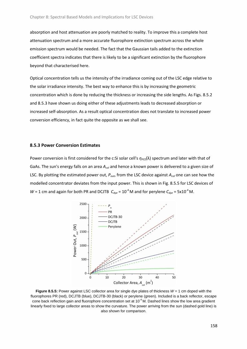
Chapter 8: Spectral Based Models and Implications for LSC Devices
158
absorption and host attenuation are poorly matched to reality. To improve this a complete host
attenuation spectrum and a more accurate fluorophore extinction spectrum across the whole
emission spectrum would be needed. The fact that the Gaussian tails added to the extinction
coefficient spectra indicates that there is likely to be a significant extinction by the fluorophore
beyond that characterised here.
Optical concentration tells us the intensity of the irradiance coming out of the LSC edge relative to
the solar irradiance intensity. The best way to enhance this is by increasing the geometric
concentration which is done by reducing the thickness or increasing the side lengths. As Figs. 8.5.2
and 8.5.3 have shown us doing either of these adjustments leads to decreased absorption or
increased self-absorption. As a result optical concentration does not translate to increased power
conversion efficiency, in fact quite the opposite as we shall see.
8.5.3 Power Conversion Estimates
Power conversion is first considered for the c:Si solar cell's ηPCE(λ) spectrum and later with that of
GaAs. The sun's energy falls on an area Acol and hence a known power is delivered to a given size of
LSC. By plotting the estimated power out, Pout, from the LSC device against Acol one can see how the
modelled concentrator deviates from the input power. This is shown in Fig. 8.5.5 for LSC devices of
W = 1 cm and again for both PR and DCJTB Cdye = 10-4 M and for perylene Cdye = 5x10⁻⁴ M.
Figure 8.5.5: Power against LSC collector area for single dye plates of thickness W = 1 cm doped with the
fluorophores PR (red), DCJTB (blue), DCJTB-30 (black) or perylene (green). Included is a back reflector, escape
cone back reflection gain and fluorophore concentration set at 10-4
M. Dashed lines show the low area gradient
linearly fixed to large collector areas to show the curvature. The power arriving from the sun (dashed gold line) is
also shown for comparison.

Chapter 8: Spectral Based Models and Implications for LSC Devices
159
From Fig. 8.5.5 there is a huge difference seen between the irradiant power coming from the sun
and the electrical power out of the LSC-solar cell combination. One can see that overall LSC power
conversion efficiencies, which shall be exhibited shortly, are of the order of a percent or so. The
gradient of the power curves is closely related to ηLSC and is seen to decrease with collector area due
to the increased self-absorption losses. Importantly there are extra losses due to the attenuation
added into the fluorophore extinction spectra in the red tail.
The dashed lines in Fig. 8.5.5 show that an array of LSC devices will perform much better than one
large one. This must be balanced against extra cost because as we decrease the collection area of
each LSC array element so as to increase the power conversion the number of array elements for a
given total collection area increases. This means more solar cell area per unit volume of
concentrator, which will increase the cost. Such matters will be considered in detail shortly.
With the power out and power in known it is a trivial matter to determine the LSC power conversion
efficiency, as in Eq. (8.3.6). This is shown in Fig. 8.5.6 as a function of the log of collector area for LSC
devices of W = 1cm. The best LSC devices in literature are also added as single data points and for
the configuration of the 7.1% device the model is run for PR as a comparison.
Figure 8.5.6: LSC power conversion efficiency against collector area on a logarithmic scale for single dye plates
of thickness W = 1 cm doped with the fluorophores PR (red), DCJTB (blue), DCJTB-30 (black) or perylene
(green). The extended extinction model is used with a back reflector, escape cone back reflection gain is added
and fluorophore concentration optimised. Some LSC devices from literature, see Table VI on page 48, are shown
for comparison (magenta shapes) and the model is run for PR under the same device configuration as the 7.1%
device (red open square).
For all the modelled plates here severe attenuation of waveguided light begins between 1 m2 and
10 m2. As has been seen by the power curves of Fig. 8.5.5 the best arrangement for a LSC installation
will be some form of array balancing efficiency against device cost. Array elements will certainly

Chapter 8: Spectral Based Models and Implications for LSC Devices
160
need to be less than 1m2 to avoid the severe losses from the extended path lengths for such large
areas.
Comparing Figs. 8.5.4 and 8.5.6 it can be seen that increasing optical concentration necessarily
results in decreased power conversion efficiency. It is not possible to determine the optical
concentration of the devices from literature shown in Fig. 8.5.6 because ηabs and ηself cannot be
calculated from the information presented in those papers. However, the PR (GaAs) device has
Copt ≈ 0.3 for ηLSC = 0.035, which means the irradiance intensity coming from the LSC edge is less than
a third of that of the incident irradiance. By comparison the devices from literature cannot have a
Copt > 1.
The best LSC devices in literature are of very small collection area, which enhances the output but
makes them unlikely to find application as a marketable device. The 7.1% device [17] is a PMMA plate
doped with PR and a yellow coumarin fluorophore, CRS040, with area Acol = 25 cm2 and thickness
W = 0.5 cm. GaAs cells were used on all four sides, which will perform better than the c:Si cells used
for the modelled curves of Fig. 8.5.6. The 6.7% device [18] is a two layer tandem LSC using
fluorophores BA241 and BA856 with Acol = 4 cm2, W = 0.3 cm and GaInP solar cells on all four sides.
The 1.3% device made back in 1981 [22] has DCM as the fluorophore at Cdye = 2.2x10⁻⁴ M, which
makes interesting comparison with DCJTB since they are of the same chemical family. DCJTB has a
higher quantum yield than DCM and was modelled here at 10-4 M so one might expect the blue
curve in Fig. 8.5.6 to sit a little above the open magenta triangle. Additionally the DCM device was
0.4 cm thick whilst the DCJTB model here is run for a 1 cm plate, which means the 1.3% device will
be absorbing less solar irradiance. This tells us that there is a significant difference between the
model and reality, despite the apparently pleasing visual comparison in Fig. 8.5.6. Another point is
that of self-absorption, which may be less for DCM and we must also consider that self-absorption
and attenuation in the model is based on an estimate, not reality.
Another reasonable comparison can be made with the 7.1% device to compare against the single
fluorophore PR LSC of the model. The c:Si ηPCE(λ) spectrum is exchanged with that of GaAs and the
fluorophore concentration is set to 1.2x10⁻⁴M. The result of this is also in Fig. 8.5.6 and the model
predicts this will device will have roughly half of that of the 7.1% device of literature. Again there is a
lot of uncertainty in the model that will account for this discrepancy and the presence of a second
dye will also increase the power conversion to some extent. The 0.6 scaling of the GaAs ηPCE(λ)
spectrum will play an important role as will other assumed parameters in the model such as ηstokes.
Additional differences lie in the electrical characteristics in the real device; for example series and

Chapter 8: Spectral Based Models and Implications for LSC Devices
161
parallel cell circuit configurations are built and also the back reflector they use has 0.97 reflection
efficiency, not unity. Despite these differences and the uncertainties in the model the results
presented here seem to lie in general agreement with that of real devices with perhaps too much
lost by the model to cell efficiency scaling and extended extinction.
The gains from solvation for DCJTB increase as collector area increases because of the steeper
increase in self-absorption seen for pure DCJTB. At about Acol = 1 m2 the enhancement of LSC power
conversion efficiency of DCJTB-30 relative to pure DCJTB is roughly 61.3%, which is significantly
greater than the 23.4% predicted in chapter 5 for DCJTB using the overlap integral, J, to
parameterise the self-absorption. Chapter 5 actually made predictions of the optical efficiency, ηopt,
but the comparison still holds since we're comparing devices of the same geometric concentration,
G. Therefore the only difference between DCJTB-30 and DCJTB is in the irradiant intensity falling on
the solar cells which is governed by ηopt.
There is an issue with this comparison; in chapter 5 the fluorophore concentration was fixed at Cdye =
0.1 wt% or 2.6x10⁻³ M, which means faster extinction. The result of increasing fluorophore
concentration at fixed Acol is to increase the gains from the solvation effect because transport losses
increase faster for pure DCJTB. For Acol = 10-4 m2 the solvation enhancement is reduced to just 13.6%
relative, which is less than that predicted using J. It can be concluded that J is a poor estimator of the
true effect of self-absorption and is a value only appropriate for very small path lengths of around 1
cm. Self-absorption is a stronger effect than characterised in chapter 5 and as a result solvation gives
rise to greater efficiency enhancements than expected from that earlier analysis.
Another effect that can be considered is that of a change in host material and hence refractive index.
Fig 8.5.7 shows LSC efficiency as a function of collector area for the fluorophore PR with several
values of n with W = 1 cm.
Fig. 8.5.7 shows, in a more detailed manner, a similar result to Fig. 2.2.4. Increasing host n results in
various changes; the amount of reflected incident irradiance increases but the escape cone shrinks
increasing the amount of trapped light. Additionally the mean path length increases with increased n
due to the introduction of extra emission rays by the reduced escape cone, which have smaller
angles relative to the LSC surface normal. Because of this the self-absorption efficiency, ηself,
decreases slightly but not significantly enough to stop higher refractive indices delivering higher
power conversion efficiencies. Changing a host material does not just change n, however, but also
host attenuation, film forming and mechanical properties must also be considered.
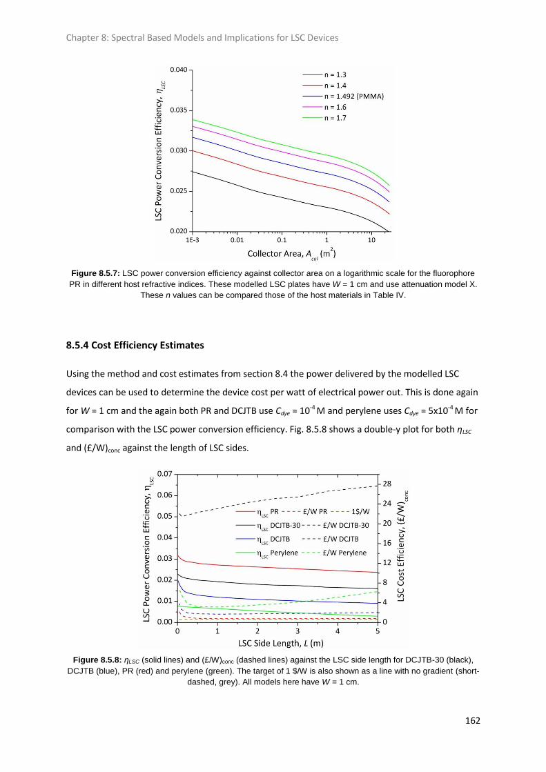
Chapter 8: Spectral Based Models and Implications for LSC Devices
162
Figure 8.5.7: LSC power conversion efficiency against collector area on a logarithmic scale for the fluorophore
PR in different host refractive indices. These modelled LSC plates have W = 1 cm and use attenuation model X.
These n values can be compared those of the host materials in Table IV.
8.5.4 Cost Efficiency Estimates
Using the method and cost estimates from section 8.4 the power delivered by the modelled LSC
devices can be used to determine the device cost per watt of electrical power out. This is done again
for W = 1 cm and the again both PR and DCJTB use Cdye = 10-4 M and perylene uses Cdye = 5x10⁻⁴ M for
comparison with the LSC power conversion efficiency. Fig. 8.5.8 shows a double-y plot for both ηLSC
and (£/W)conc against the length of LSC sides.
Figure 8.5.8: ηLSC (solid lines) and (£/W)conc (dashed lines) against the LSC side length for DCJTB-30 (black),
DCJTB (blue), PR (red) and perylene (green). The target of 1 $/W is also shown as a line with no gradient (short-
dashed, grey). All models here have W = 1 cm.

Chapter 8: Spectral Based Models and Implications for LSC Devices
163
For small scale devices, such as the best in literature discussed earlier, the LSC efficiency is at a peak
due to minimised self-absorption losses. This declines quickly to the regime where self-absorption
saturates except in the extended red tail of extinction, which causes a slower decline in ηLSC with
increased L. At around L = 0.3 m the cost efficiency reaches a minimum which holds for PR, DCJTB
and perylene up to 1 or 2 metres. PR has a minimum of (£/W)conc = 0.76 £/W at around L = 1.7 m;
this length will not give the best power conversion efficiency for the LSC but will deliver the best
economics. According to these models a single dye LSC based on PR should perform at double the
cost per watt as a c:Si solar module. An array of LSC devices using PR based on the results here
would be made of square LSC devices with a side length of 1.7 m. At this size each plate, with c:Si
cells attached, is generating around 160 W and the collector area is Acol = 3 m2. That gives
approximately 53 W/m2 for a total device cost of £120. By contrast a modular c:Si solar panel
generating 160 W/m2 and costs around 0.61 £/W; therefore for an area of Acol = 3 m2 such a panel
would generate 480 W and would cost about £293. It is less costly to cover a larger area with LSC
devices based on PR but the result is less power and poorer economics of wattage.
The cost per watt of power out is seen to be higher at very small L due to the way in which the
different costs vary with LSC geometry. Consider Eq. (8.4.1); the cost of solar cells depends on edge
area, Ahar = 4LW, whilst the host and dye materials depend on LSC volume, VLSC = L2W. Therefore,
since volume grows faster than harvesting area, the costs from host and fluorophore materials will
dominate very quickly. At small lengths L2 is very small and the cost of the cells will dominate, except
in the case of DCJTB-30 using nanoparticles. This is seen in Fig. 8.5.9.
Figure 8.5.9: Log-log plot of costs in pounds (£) for the concentrator (solid lines) and solar cell (dashed line)
components of a W = 1 cm LSC device as a function of LSC side length. DCJTB-30 (black), DCJTB (blue), PR
(red) and perylene (green) dyes are shown.
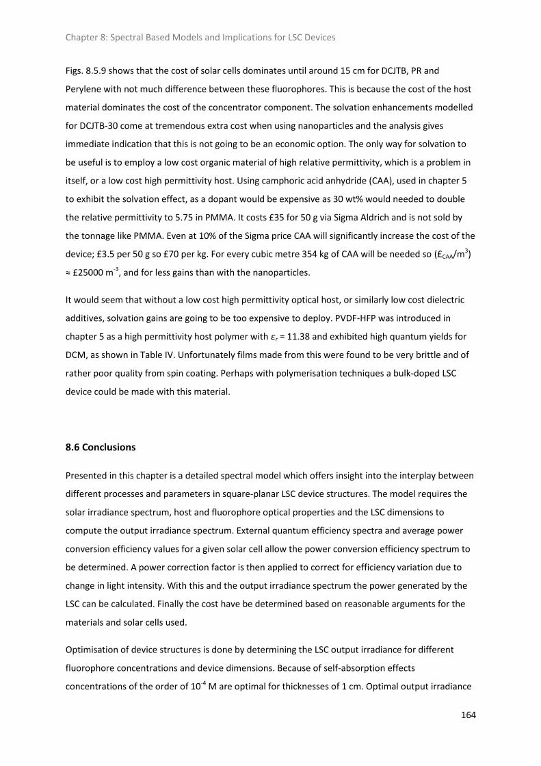
Chapter 8: Spectral Based Models and Implications for LSC Devices
164
Figs. 8.5.9 shows that the cost of solar cells dominates until around 15 cm for DCJTB, PR and
Perylene with not much difference between these fluorophores. This is because the cost of the host
material dominates the cost of the concentrator component. The solvation enhancements modelled
for DCJTB-30 come at tremendous extra cost when using nanoparticles and the analysis gives
immediate indication that this is not going to be an economic option. The only way for solvation to
be useful is to employ a low cost organic material of high relative permittivity, which is a problem in
itself, or a low cost high permittivity host. Using camphoric acid anhydride (CAA), used in chapter 5
to exhibit the solvation effect, as a dopant would be expensive as 30 wt% would needed to double
the relative permittivity to 5.75 in PMMA. It costs £35 for 50 g via Sigma Aldrich and is not sold by
the tonnage like PMMA. Even at 10% of the Sigma price CAA will significantly increase the cost of the
device; £3.5 per 50 g so £70 per kg. For every cubic metre 354 kg of CAA will be needed so (£CAA/m3)
≈ £25000 m-3, and for less gains than with the nanoparticles.
It would seem that without a low cost high permittivity optical host, or similarly low cost dielectric
additives, solvation gains are going to be too expensive to deploy. PVDF-HFP was introduced in
chapter 5 as a high permittivity host polymer with εr = 11.38 and exhibited high quantum yields for
DCM, as shown in Table IV. Unfortunately films made from this were found to be very brittle and of
rather poor quality from spin coating. Perhaps with polymerisation techniques a bulk-doped LSC
device could be made with this material.
8.6 Conclusions
Presented in this chapter is a detailed spectral model which offers insight into the interplay between
different processes and parameters in square-planar LSC device structures. The model requires the
solar irradiance spectrum, host and fluorophore optical properties and the LSC dimensions to
compute the output irradiance spectrum. External quantum efficiency spectra and average power
conversion efficiency values for a given solar cell allow the power conversion efficiency spectrum to
be determined. A power correction factor is then applied to correct for efficiency variation due to
change in light intensity. With this and the output irradiance spectrum the power generated by the
LSC can be calculated. Finally the cost have be determined based on reasonable arguments for the
materials and solar cells used.
Optimisation of device structures is done by determining the LSC output irradiance for different
fluorophore concentrations and device dimensions. Because of self-absorption effects
concentrations of the order of 10-4 M are optimal for thicknesses of 1 cm. Optimal output irradiance

Chapter 8: Spectral Based Models and Implications for LSC Devices
165
depends on device thickness, because absorption of solar irradiance must be maximised, but also on
side length and hence mean path length because of self-absorption effects. The application of back
reflectors also plays a role, because this doubles the effective absorption length. This means thinner
devices and higher G values for the same absorption efficiency.
Although GaAs PV cells were seen to be most appropriate in terms of collecting LSC output
irradiance, the bulk of modelling was done with the c:Si power conversion efficiency spectrum. This
is because c:Si cells are widely available and likely to provide lower cost estimates. Compared to
devices in literature the model provides slightly lower estimates than might be expected. Devices in
literature only provide single data points so available empirical evidence is currently small.
Cost efficiency estimates show that the best modelled structure was using PR with a LSC side length
of L = 1.3 m and thickness W = 1 cm. This gave a cost efficiency of (£/W)conc = 0.76 £/W, double the
target of 1 $/W (0.61 £/W). Such LSC plates in an array would cover a larger area for lower cost than
a c:Si module solar field but would deliver about a third of the power and poorer economics.
8.7 References
[1] W. G. J. H. M. van Sark et. al., Luminescent Solar Concentrators - A Review of Recent Results, Opt.
Exp. 16, 26, 21773 (2008)
[2] A. J. Chatten, K. W. J. Barnham, B. F. Buxton, N. J. Ekins-Daukes and M. A. Malik, Quantum Dot
Solar Concentrators, Semiconductors 38, 8, 909 - 917 (2004)
[3] A. J. Chatten, D. J. Farrell, C. M. Jermyn, P. A. THomas, B. F. Buxton, A. Büchtemann, R. Danz, and
K. W. J. Barnham, Thermodynamic Modelling of the Luminescent Solar Concentrator, Proc. 31st IEEE
Photovoltaic Specialists Conference, pp. 82-85 (2005)
[4] A. J. Chatten, D. J. Farrell, R. Bose, M. G. Debije, A. Büchtemann, and K. W. J. Barnham,
Thermodynamic Modelling of Luminescent Solar Concentrators With Reduced Top Surface Losses, in
Proc. 22nd European Photovoltaic Solar Energy Conference, pp. 349-353 (2007)
[5] G. Colantuono, A. Buckley and R. Erdélyi, Ray-Optics Modelling of Rectangular and Cylindrical 2-
Layer Solar Concentrators, J. Light. Tech. 31, 7, 1033-1044 (2013)
[6] S. J. Gallagher, P. C. Eames and B. Norton, Quantum Dot Solar Concentrator Behaviour, Predicted
Using a Ray Trace Approach, J. Ambient Energy 25, 47-56 (2004)

Chapter 8: Spectral Based Models and Implications for LSC Devices
166
[7] R. Bose, D. J. Farrell, A. J. Chatten, M. Pravettoni, A. Büchtemann, J. Quilitz, A. Fiore, L. Manna
and K. W. J. Barnham, Luminescent Solar Concentrators: Nanorods and Raytrace Modelling, 33rd.
IEEE Photovoltaic Specialists Conference, pp. 1- 5, (2008)
[8] R. Bose, D. J. Farrell, A. J. Chatten, M. Pravettoni, A. Büchtemann and K. W. J. Barnham,
Luminescent Solar Concentrators: Cylindrical Design, Proc. 24nd European Photovoltaic Solar Energy
Conference, pp. 359-362, (2009)
[9] A. Goetzberger and V. Wittwer, Fluorescent Planar Collector-Concentrators: A Review, Solar Cells
4, 3 – 23 (1981)
[10] W. R. L. Thomas, J. M. Drake and M. L. Lesiecki, Light transport in planar luminescent solar
concentrators: the role of matrix losses, Appl. Opt. 22, 12, 3440-3450 (1983)
[11] K. R. McIntosh, N. Yamada and B. S. Richards, Theoretical Comparison of Cylindrical and Square-
Planar Luminescent Solar Concentrators, App. Phys. B 88, 285-290 (2007)
[12] O. Y. Edelenbosch, M. Fisher, L. Patrignani, W. G. J. H. M. van Sark and A. J. Chatten,
Luminescent solar concentrators with fiber geometry, Optics Express 21, S3 (2013)
[13] M. A. Green, K. Emery, Y. Hishikawa, W. Warta and E. D. Dunlop, Solar Cell Efficiency Tables
(Version 38), Prog. Photovolt: Res. Appl. 19, 565-572 (2011)
[14] M. A. Green, K. Emery, Y. Hishikawa, W. Warta and E. D. Dunlop, Solar Cell Efficiency Tables
(Version 39), Prog. Photovolt: Res. Appl. 20, 12-20 (2012)
[15] M. A. Green, K. Emery, Y. Hishikawa, W. Warta and E. D. Dunlop, Solar Cell Efficiency Tables
(Version 44), Prog. Photovolt: Res. Appl. 22, 701-710 (2014)
[16] NREL, AM1.5 Direct Irradiance Spectrum, Excel Data,
http://rredc.nrel.gov/solar/spectra/am1.5/
[17] L. H. Slooff, E. E. Bende, A. R. Burgers, T. Budel, M. Pravettoni, R. P. Kenny, E. D. Dunlop and A.
Büchtemann, A Luminescent Solar Concentrator with 7.1% Power Conversion Efficiency, Phys. Stat.
Sol. (RRL) 2, 257-259 (2008)
[18] J. C. Goldschmidt, M. Peters, A. Bösch, H. Helmers, F. Dimroth, S. W. Gunz and G. Willeke,
Increasing the efficiency of fluorescent concentrator systems, Sol. En. Mater. Sol. Cells 93, 176 - 182
(2009)

Chapter 8: Spectral Based Models and Implications for LSC Devices
167
[19] E. E. Bende, L. H. Slooff, A. R. Burgers, W. G. J. H. M. van Sark and M. Kennedy, Cost & Efficiency
Optimisation of the Fluorescent Solar Concentrator, in Proc. 23rd European Photovoltaic Solar
Energy Conference (2008)
[20] Personal communication, in light of [19], with A. J. Cadby, University of Sheffield (2014)
[21] R. Bose, D. J. Farrell, A. J. Chatten, M. Pravettoni, A. Büchtemann, J. Quilitz, A. Fiore, L. Manna, J.
Nelson, A. P. Alivisatos and K. W. J. Barnham, The Effect of Size and Dopant Concentration on the
Performance of Nanorod Lumienscent Soalr Concentrators, Proc. 23nd European Photovoltaic Solar
Energy Conference, (2008)
[22] J. S. Batchelder, A. H. Zewail, and T. Cole, Luminescent Solar Concentrators 2: Experimental and
Theoretical Analysis of their Possible Efficiencies, Applied Optics 20, 21, 3733 - 3754 (1981)
[23] L. Desmet, A. J. M. Ras, D. K. G. de Boer and M. G. Debije, Monocrystalline silicon photovoltaic
luminescent solar concentrator with 4.2% power conversion efficiency, Opt. Lett. 37, 15, 3087 - 3089
(2012)

168
Chapter 9
Conclusion
9.1 Summary
Over the preceding five chapters the major experimental work of this research project has been
discussed in detail. The findings are summarised here first before framing the results in the context
of luminescent solar concentrator devices and their place in the wider energy market.
In chapter 4 a Gauge R & R (GRR) study design is used on the absolute measurement of fluorescence
quantum yield using an integration sphere so as to assess different sources of variance in the
process. The GRR study shows that most of the variance lies within the measurement system rather
than in sample fabrication. Fluctuations in laser intensity were found to be the largest source of
variance to the total uncertainty in the measurement, although some systematic uncertainty due to
calibration and self-absorption corrections could not be ruled out, even when using the light
emitting polymer F8 as a fluorescence standard. The more stable GaN laser excitation source was
found to achieve a minimum uncertainty on the ηQY of ±0.01. Simultaneous measurement of the
excitation intensity and sample emission, using a beam splitter and second photodetector, would
allow the laser uncertainty to be made negligible. Improving the accuracy of this measurement is an
important goal for optical characterisation, particularly for fluorophores with near unity ηQY.
In chapter 5 improvements in the self-absorption efficiency, ηself, are shown to be possible using the
solvation mechanism in the solid state. This phenomenon occurs for particular fluorophores where
the molecular dipole moment increases upon absorption of a photon. This in turn causes the
surrounding medium to readjust physically and electronically around the new dipole state and in
turn this sets up a reaction field which takes energy from the excited state, shifting the emission
spectrum towards lower energies. By introducing high permittivity small organic molecules into
PMMA along with DCM class fluorophores an improvement in optical efficiency of up to 25% is
shown to be possible when using the overlap integral, J, as a metric for self-absorption. Later on, in
the spectral analytical models of chapter 8, this metric is seen to be far too conservative and much
greater improvement in optical efficiency is predicted in that work. However, the cost efficiency
analysis in chapter 8 indicates that finding suitable dielectric dopants of low enough cost is likely to
be one of the biggest obstacles to employing this method.
Chapter 9: Conclusion
169
In chapter 6 a Prism Ultra-Coat 300 spray-coating deposition tool is assessed for its efficacy in
producing thin films for bi-layer LSC devices. A screening study design of experiment is employed to
assess the influence of different input factors on the deposited film quality. Quality is characterised
by seven response metrics which describe roughness, absorption of incident light and self-
absorption of waveguided light. The deposition system offers low control of roughness but typical
values of the relevant response metrics are in the range of acceptable levels of surface roughness.
Low control is also seen for the self-absorption metrics, which is to be expected since this
phenomenon depends primarily on path length through the waveguide and fluorophore properties,
not on the deposition method itself. In terms of film thickness, and hence absorption of incident
light, the spray coater offers good control in a limited range, which is significantly less than that
required to achieve optimal absorption efficiency, even considering use of back reflectors.
Ultimately, because of constraints on the possible film thickness and on the fluorophore
concentration, this spray-coating deposition system is found to be unsuitable for delivering the
requirements of a bi-layer LSC device. It is thus unclear whether spray deposition would work for bi-
layer LSC devices.
In chapter 7 an exploration of concentration quenching is exhibited showing results of fluorescence
quantum yield and lifetime studies. Different fluorophores are seen to exhibit different forms of
quenching response in terms of range (r dependence) and strength. Explorations of a variety of
organic polymer host materials gives strong indication that the host environment also plays a big
part in stabilising fluorophore excited states. By exploring the quenching rate as a function of
molecular separation for DCM and C102 in the PMMA host the form of the quenching response is
conjectured to be the empirical result of different interactions. The magnitude of the monomial
power law determined for the quenching rate indicates that point-like dipole-dipole deactivation
interactions, as in FRET, are not the sole responsible mechanism of concentration quenching. Other
forms of photophysical interaction are considered to explain this discrepancy including surface-
surface and point-surface electronic interactions.
Finally in chapter 8 a spectral based analytical model for estimating LSC performances is described
and discussed. The AM1.5 solar irradiance spectrum is used under normal incidence to the LSC
collection face of a square-planar LSC geometry. Transmission and absorption of this solar irradiance
are considered through host optical properties, LSC thickness and fluorophore extinction
coefficients. With the quantum yield and normalised emission spectrum of the fluorophore a
corrected equivalent intensity irradiant output is generated from the absorbed irradiance. Trapping
efficiency and transport losses, due to both the matrix and self-absorption by the fluorophore, are
Chapter 9: Conclusion
170
then factored into the model so that an LSC output irradiance spectrum is generated for three
orders of emission. This output irradiance is coupled with c:Si or GaAs solar cell power conversion
efficiency (PCE) spectra to determine the power generated by the modelled LSC device. The LSC PCE
can then be calculated and the cost efficiency determined using reasoned values for the costs of
each LSC component; the host, dye and solar cells.
The spectral models of chapter 8 show that current fluorophore technology can at best achieve
roughly double the 1 $/W cost competitiveness of c:Si modules already on the market.
Advancements in fluorophore technology have not translated to much better LSC devices in
literature. A comparison of the model with LSC devices from literature finds some level of agreement
in the power conversion efficiencies but also that real devices do not occupy a large parameter
space, making it harder to justify the model. Almost all literature devices are square-planar LSC
devices with one or two fluorophores in single plate LSC designs. Many are small in size, particularly
the newest devices, which drives up efficiencies because of reduced light transport losses.
Furthermore the newest devices use solar cells that are better suited to the LSC output spectrum
and so in real terms the improvement in empirical LSC devices is smaller than a first glance would
suggest.
9.2 Implications for LSC Devices
As stated in chapter 1.3 LSC devices are unlikely to see a main role in the global solar energy market.
This is borne out by the models of chapter 8 which show low power conversion efficiencies (PCE) and
poorer economics than competing solar energy technologies. The main costs of LSC devices are
shown to be dominated by the host and dye materials for devices larger than five centimetres in side
length. Therefore to reduce LSC costs most significantly the host and dye materials need to be
synthesised and processed at as low a cost as possible. Including any new components such as extra
dye materials, multiple stacks, more expensive solar cells or photonic band stops will ultimately
result in increasing the device cost.
Current fluorophore technology does not offer the high photostability, high quantum yield, low self-
absorption and strong absorption of the solar spectrum that LSC devices require. The best
fluorophores offer near unity quantum yield for low concentrations, ideal for bulk-doped LSC
structures, but still exhibit strong overlap of absorption and emission spectra. The solvation
mechanism was considered to alleviate this problem but has been shown to introduce too much

Chapter 9: Conclusion
171
extra expense due to the cost of high permittivity dopants. Development in low cost, high
permittivity host materials and suitable fluorophores could solve this and make the technique viable.
The absorption of solar irradiance remains one of the biggest challenges facing fluorophore
technology with single dye systems typically able to absorb up to 30 to 35% of solar energy. If all the
solar energy up to 750 nm could be absorbed then that would give an absorption efficiency of 54%
for AM1.5 irradiance. A concerted, exhaustive effort to explore novel fluorophore compounds is
needed to push absorption efficiency up and ultimately test whether all the requirements on LSC
fluorophores are feasible. Quantum chemical modelling seems an appropriate way to search for
suitable fluorophores without having to synthesise them and test their individual properties.
Current host materials do not offer high enough refractive indices, n, which could increase power
conversion efficiency by up to 10% relative to PMMA, for n = 1.7 or more. Also transport losses due
to host matrix related attenuation must be minimised. Considering the concentration quenching
results of chapter 7 the properties and interactions of the host with the fluorophore also need to be
understood better with a view to improving fluorophore stability and emission efficiency. A more
detailed investigation of quenching processes for different hosts with various fluorophores would be
a step towards this.
In final conclusion LSC devices do not yet offer the power conversion and cost efficiencies required
for marketable devices. The models of chapter 8 suggest that arrays of LSC plates may already find
place in niche market roles such as energy windows, paving slabs and awnings. Such systems, if the
models are correct, could currently generate around 50 W per m2 of LSC plate doped with PR, under
normal incidence AM1.5 irradiance and using c:Si cells. These would cover any given area for less
cost than c:Si modules and could easily be integrated into structures. The power delivered would be
a third of that for PV collection under direct solar irradiance. The hypothetical installations proposed
would probably need the concentrator plate replacing every two years or so, though the c:Si cells
will last much longer. How long the solar cells will last for under LSC output irradiance is another
question. Further research and development is really needed to mature the technology before even
the above niche markets are considered.