optimal control of execution costs for portfolios

OPT^ CONTROL OF EECUTION COSTS FOR PORTFOLIOS The authors apply stochastic dynamic programming to derive trading strategies that minimize the expected cost of executing a portfolio of securities over a fixed time period. They test their strategies using real-world stock data.

he rapid growth in equity investing, driven by the increasing popularity of mutnal fiinds and defined-contri- T hution retirement plans, has led to a

rising concentration of assets among institutional money managers. A typical portfolio inaiiager now oversees a large portfolio of several hundred securities, with individual positions that might constitute a significant fraction of the security’s average daily volume. Both active managers and passive indexers must frequently rebalance their portfolios, to include new stock picks, to sell stocks that are out of favor, or to improve the tracking of a given index or benchmark, This generates sizeable orders across inany stocks that must be cxccuted within a relatively short time horizon, and that innst be executed together so as to maiiitain the portfolio’s risvreward charac- teristics. The transaction costs associated with trading such “lists” of securities-often called execution costs-can he substantial.

Execution costs have several components: explicit costs such as coinmissions and bid/ask spreads, and costs that are harder to quantify, such as the oppmzmity cmt of waiting and the price

1521-96151991110.000 1999 IEEE

impact from trading. @porhinity costs arise because market prices are moving constantly and can move favorably or unfavorably without warning, generating unexpected profits or lost opportunities while a portfolio iiianager hesi- tates. Price impact is the typically unfavorable effect on prices that the act of trading creates, not unlike the turbulence that a ship’s wake gcn- erates. A security’s seller will, by the very act of selling, push down the security’s price, yielding lower proceeds from the sale, and siniilarly for tlie buyer. Moreover, the larger the order, tlie more hcavily the trade affects the price. For portfolios that turn over frequently or havc large positions to trade, these costs can significantly hinder the fund’s overall pcrfonnance.’

Reccnt studies show that institutional investors often break up their larger trades into smaller “packages” that they execute over the course of several days.2-s There is a coinpelling ccononiic rationale for package trading. lrading is fundamentally a dynamic, patli-dependent, stochastic problem. Trading takes time, and the act of trading affccts price and price dynamics, which, in turn, affect execution costs. Control- ling the execution costs of large blocks of stock inust he accomplished by trading over a nuinher of time periods. This was recognized by Dirnitris Bcrtsinias and Andrew Lo, who used stochastic dynamic-progrdinining techniques to

‘I’his article was cditcd to CiSE hriuse style siid space IC- quircmciits. Far the full vcrsian, contact Andrew Lo a t thc addrcss listed for him on p. 23.

40 COMPUTING IN SCIENCE 61 ENGINEERING

derive optimal or be.rt-execution strategies.‘ In this article, we extend the single-asset

framework Bertsirnas and Lo outlined, to coli- struct hest-execution strategies for portfolio problems. Wc devcloped a specification for these problctns that is both einpirically plausible and coinputationally tractable to implcment. T h e closed-form solution provides insight into the naturc of trading portfolios. To quantify the potential cost savings of our strategies, we fit the parameters of our price-impact model using his- torical data on 25 large-cap New York Stock Ex- change (NYSE) stocks.

The portfolio problem Specifically, wc solve this problem:

given fixed blocks of shares in E stocks, 5 = [it Sz . . . in]’, to be purchased within a fixed finite number of periods T, and given a set of pricc dynamics that capture price impact (that is, an individual trade’s execution price as a function of the shares traded and other “state” variables), find the optimal qzmm of trades (as a hnc- tion of the state variables) that minimizes the cxpccted cxecution costs.

Because, as is wcll-known, the short-term de- inand curves for even the most actively traded equities arc not perfectly elastic,’ a market order at date 0 for the entire blockfis clearly not an optimal trading strategy.

(we follow the cotninon convention that all vcctors are column vectors unless they are ex- plicitly transposed, and boldfacc Roman antl Greek letters denote vectors and matrices. For simplicity and without loss in generality, we consider the case of pmchasingfonly. SellingS and a combination of buying certain stocks and selling others can easily he accommodated with the appropriate sign conventions [positive numbers for purchases, negative for sales].)

Let r, = [.rIl, I*,, . . ., S ~ J be the number ofsharcs of each stock acquired in period t at prices p t = {PI,, I]*,, ..., p.,], where t = 1, .._, T. We can ex- press the investor’s objective as

subject to

C S , = 5 (2) t= l

whcre x, is a vector of state variablcs, E, is vector white noise, andff) and g(.) are the state equations or laws of motion that incorporate the price dy- naniics ofpt, the price impact of trading s,, and the dynamics of the state variables. Wc might also wish to impose additional constraints-for exatn- ple, a no-sales constraint, s, t 0-or othcr conditions that are placed on the portfolio manager by institutional restrictions, tax considerations, or other aspects of his or her investment process.

(If a portfolio managcr is attempting to ac- quire a block of securities, selling the same securities during the acquisition pcriod is difficult to justify Lunless, of course, the manager has ex- tremely accuratc neptive information rcgard- ing the security’s price, which is somewhat in- consistent with thc original premise that he is a buiycr]. Indeed, in inany cases, it is illegal because it is considered a violation of the fidnciary trust that portfolio managers have to act in the hest interests of their investors.)

T h e portfolio casc contains several interesting feahlrCS that the single-stock analysis of Bertsi- mas and Lo and others did not capture. Perhaps the most inqiortant feature is the ahility to cap- hire cross-stock relations such as the cross-auto- correlations rcported t)y Andrew Lo and Craig MacI(inlay.* Price niovetnents in one stock can induce similar movements in the price of another, hecausc of cithcr common factors driving both or linked trading strategies-for cxatnple, pairs trading, index arbitragc, antl risk arbitrage. In such cases, the price impact of trading a portfolio might he larger than thc sum of the price impact of trading the individual stocks separately.

Altcrnatively, if some stocks are ncgatively correlated (perhaps because of portfolio suhsti- tution effects) or if the portfolio to be executed includes both purchases and sales, thc portfolio execution cost might be lower than the sum of the individual stocks’ execution costs. This is because of a diversification effect in which trades of one stock lower the price impact of trades in anothcr. Whether execution costs are magnified or mollified in the portfolio case is, of course, an empirical issue that turns on the law of motion for the vector of prices and state variables. In either case, the portfolio setting clearly is considerably tnorc complex than the single-stock case.

The state equations We now present a specification for the state

equations that incorporates a multivariate price- impact fuiiction with cross-stock interactions.

Let the execution priccp, he the sum of two components:

where 3, is a “no-impact” price-the price that would prevail in the ahsence of any market impact-and 6, is the impact. A plausible and ob- servable proxy for the no-impact price is the midpoint of the hid/offer spread, although it can he arbitrary so long as the trade size s, does not affect it. For convenience, and to ensure nonnegative prices, we model fit as vector-gcoinet- ric Brownian motion:

where 2, is a diagonal matrix whose diagonal is a normal random vector zt with mean p z and covariance matrix 4. The exp(.) operator denotes the matrix exponential, which, in this case, reduces to the element-wise exponential of the diagonal entries in Z,.

For 6, we set

S, = P,(APts, + Bx,) , ( 5 )

where PI = diag[jiJ and diag(.) is the diagonaliza- tion operator that maps its vector argument into a diagonal matrix with the vector as the diagonal. This spccification caphlres the impact of trading s, shares on the transaction prices pp It also implies that as a percentage of the no-impact price, j t , the price impact is a linear function of the dollar value of the trade and other state variables xt. The price impact’s form (see Equation 5 ) differs from the single-stock case in that the percentage price-impactfunction for each stock i is a linear function, A’$,, of the dollar values of the wades of all n stocks, not just of stock i. In the special case where A is diagonal, the portfolio problem reduces to n independent single-stock problems solved by Bertsimas and Lo?

This specification of the dynamics ofp, has several advantages over other specifications (see the “Other specifications” sidebar). First, 3, is guaranteed to be noiinegxtive, andp, is guaranteed to be nonnegative under mild restrictions on 6,. Second, separating the transaction price pt into the no-impact componentp, and impact coinpo- ncnt 6, makes the trade’s price impact temporary So, the impact affccts the current transaction price hut docs not affect future prices. Third, the

percentage price impact increases linearly with the trade size, which is empirically plausible.'^"'' Fonrth, Equation 3 implies a nattiral decomposition of execution costs, decoupling market- microstructure effects from price dynamics, which is closely related to AndrC Peroldh notion of implementation shortfall.l2 Finally, we shall see in “The dynamic-programming solution” section that Equation 3 admits a closed-forin solution in which the best-execution strategy is a simple linear function of the state variables and in which the optimal-value function is quadratic.

(Because Equation 3 implies that price inipact is temporary, affecting onlyp, and notfi,, the objective function [see Equation 11 separates into two terms. The first is the no-impact cost of execution and the second is the total impact cost. This decomposition is precisely the one Perold proposed in his definition of implenientation shortfall, but we apply it to executingi In particular, the first term gives the “paper” return or execution cost, and the slim of the two terms gives the actual cost. So the second term is the implementation shortfall in executing i.)

The presence of the vector xt in Equation 5 capturcs the potential influence of changing market conditions or private information about the securities on the price impact 6,. For example, xI might be the return on the S&P 500 index, a common component in the price of most equities. We model xt as a vector with Y elements, allowing for multiple sources of information to influence execution prices (or several lags of a single state variable).

To complete our specification of the state equation, we must specify the dynamics of x,. For simplicity, we let

xt = cx,. I + U*, (6)

where 7, is vector white noise with mean 0 and covariance matrix C,. Because xt is a vector au- toregressive process with one lag (an “AR(l)”), we can capture varying degrees of predictahility in inforination or market conditions. The matrices A and B measure the price impact’s sensitivity to trade size and market conditions. A must be positive definite; B is arbitrary; C must have eigenvalues less than unity in modulus (to ensure stationary of x,).

The dynamic-programming solution We use a stochastic dynamic-programming al-

gorithm to solve the optimal-execution problem

42 COMPUTING IN SCIENCE & ENGINEERING

(see Equation 1). We denote by w, the vector of shares remaining to be bought (or sold) at time t:

WI =s

w'7.+1 = 0 w, = wt-i -si+,

WI = s W?'+] = 0 Linear-percentage price impact

As with all dynamic-programming solutions, we begin a t the end. V, is the optimal value function a t the end of onr trading horizon, period T. By definition,

T h e condition w , ~ ~ = 0 ensures that a11 S shares are cxecuted hy time T. Thc conipletc statement of thc problem is then

Vr(j&,xT,w7.) = M~E,[p&] = ET[p;w.,.]

I NOVEMBER/DECEMBER 1999 43

= [p,.( e,2 + AP, wl. + nz,. ,]'w,. subject to

(7 )

Because this is the last period and w, , ;~ i t l u s t be sct to zero, thc remaining order wT must execute. So, the optimal trade size s+= WT. Becausc &= pT, we can reexprcss Equation 7 as

. . . state eq.at om" in tne ma'n article is oniy v

ole spec fico: IS. For examp e, Dimctris Eer ' mas and Aii- drew Lo' pi ,se a natural multivariate extension of their "in- ear pr'ce ims I specificat on in wnich the state equation is

pr = pr. I Art T Bx, T €1, (A) where A is a posit've clef nite n x n matrix, B ;s an arbitrary 11 x n l matr x. x , is an rn vector of information variaoles, ana t, is n-vector wnite noise w'th meail 0 ana covariance m a t h Xe As before, we assume Ilia1 x , follows d stationary AR(1) process. So,

where C s an rn 4 m matrix with eigenvalLes all less than miry in moaulu:, and 11, IS rn-vector whte no se with meail 0 and cokariance matrix X,, and which is ndependent of e..

Tnir spec'fication dffers I gnilicantly from the linear- percentage price impact in three bas'c respects. Perhaps the most important aifference 'I that EqLar on A imp.ies that the price 'mpact has a "permanent" elfecl on prices, oecatise of the random-walk nature of me price d) narnics. Also. the prcc

tne same dol ar impact on a $1 stock as it w'll on a 31 00 stocd. Finally, un err some ratner unnatural restrictions are placed on E, in EqLatiun A, p, CO&O lane on negative vaILes- clcar y an unrea istic prospect.

01 course, Bertsimas and Lo consider Equat;on A primarily for analytic tractability, not oecause of supporting empirical er'dencc.' luevertheless, it is instructive to compare tnis speci-

of mdiiy possi- state equation. In practice, the sute eqmtion must be erti- mateu empir'cally. For example, several empir cai stJd'es secin IO point to both permanent and temporary price impact in LS equity data.'" However, given the evcr.changing nature of f'nancia markets, 't is cruc'al to reestimate tne state equation for each app ;cat 011 .sing the most recent data sets avel.able.

References I. D BSN rmd$ an" A. -0. 'Opl'ma C~nlro 01 Ekacut on Corti. A Stud) of

Caurmmmi Bonds w'th me S a m MIILIII, Dale ' I, f.mm o Atorheir,

2 M Bsclay an0 R .limberger, "AnnoLncemeiil fffr'rr,olhew Eq. 0 w e , ana the "re of Incrdda, Pr'm Data ' , f nom01 fconomicl do 21

1908 pp 71-100

3. M.Barca, I?", Hainer 'SleilrnlrrangandVulai; I):HnthTradec

M m c P r m ? / Fr'ont'o Iconomrr. "01 34. 1993. pp.281-306.

4. 1 Cnan nnu I. Laionisnu6 ' niiit-1 onal Traaes and Inira.Day Stor" Pr <e

(6) \ 0 1 1,ha 1 .30Apr .1998pp 1-50 xi = cx ,.I + vi,

Ben.+ior,'~ fnonca fwrmar,Vol 31 1993 p)1.173-199.

5 . Chnn dnd I. .J!.OU mob 'Tnr Behnr'or 01 Srou PI .er I~OLIIICI nrl IL-

mpact IS linear, mplying that a 10,000-snare trade will have tiona TWOZI.', rnoncp v0.50 1995,pp 1147-1174.

6. R ho dla.ren. R L d r u . tn. an0 D Ma)err. 7ne Wecl nf a g e Block

Tranm.l on5 an S e c d t y Pr cec A Cro,r-Strlmna Ana ,%'%'', hnao<b

f.onomics, \01 19 IYn?. pp 237-267.

7 R. noltndurm. H Len\r~n, m o D hlayerr ' a g e B ock TianSdcliOm !ne

Speeo of Rripome ana Temporaq ma Permanent SluCK-PMc Ellecu. I f,n.mral tmnoilli~l. VoI.Zb. 1990 pp 71-95.

8 n K r u a r o ~ 1 . 5~011. 'Yrce mpaUroIBoc.Tratl nqnn me he* \ark

VT(pT,xT , U T ) - I I

= e:,PTwT + w+RrA'PTw7. +x; .B'PrwT,

which shows that the optimal value function is linear in xT and linear-quadratic in w?; By con- tinuing recursively in this fashion and applying Bellman's principle of optimality,13 we find that the optimal value function V,-, is

VT-(. = iMinF.,-,[p+-p-(. + V,._(.,, lS.l-,.l

( p ' / ' - k + 1 2 x 7 - k + l , wT-h+l) l

= e:,D,,,e,, + e:Dr,,e, + eiE,x.,_, + xk.,F,e,, t x;.,G,x,.-, + x ; . ~ , H , w , . ~ ,

+ w.~ . . l~T . IxT .k + elK,w>-, +

+ w;-,N,w,-, (8)

This yields the hest-execution strategy

' T - k = Az,(.xT-(. + A w ( . w T - k + A l , k e u (9)

(For explicit expressions for Q,k, D,;,, E&, Fk, Gk, Hk,J(., 4, Lk, ami Nk, and for Ax,,, 44 and Alp, see the Appendix posted at http://coniputer. org/cise.) T h e recursion (see Equation 8) and best-execution strategy (see Equation 9) coin- pletely characterize the solution to our original problem, and yield the expected best-execution cost, Vpk, as a by-product.

Linear price impact Under the law of motion (see Equations A and

B in the sidebar), Bertsimas and Lo6 show that the portfolio problem (see Equation 1) can be solved with Bellman's equation, which yields the following hest-execution strategy,

..;.-, = ( I - L 4 i ! l ' 4 0 w T ~ k +-A,&IB;.ICx 1 -1 .,.. ,, 2 2

(10) and optimal-value function,

VT-(.(~T-,.~I,X?.~,,W.,~~~) = P; . - ( . -~WT_, + W+-p4(.W~-k

+x;.-kn(.wT-I + X ; - , C , X ~ - ( . t (1,

for k = 0, . . ., T- 1, where

I A -A--AA;!,A' , 4

1 I

2

A, = A (.-

B , =-cB,-,(A;,-,)- A'+B', n, = n'

1

4 C, = C ' C , ~ , C - - C ' U , ~ , ( A ~ , ~ l ) ' ~ ' B , . l C , C,, = O

d, = d , - , +I',[?J;.~iC,~lO1.~,], d , = O

The best-execution strategy (scc Equation 10) is qualitatively similar to the optimnl single-stock strategy of Bertsimas and Lo.' However, it has one key difference: in the portfolio case, unless the matrix A is diagonal, the best-execution strategy for one stock will depend on the parameters and state variables of all the other stocks. To see this, observe that the matrix coefficient

tnultiplying w,_, in F.quation 10 will generally not he a diagonal matrix unless A is diagonal. Of course, if A is diagonal, trading in one stock has no price impact on any other stocks (see Equa- tion A in the sidebar). So, the portfolio problem essentially reduces to n independent single-stock problems.

So, whether the portfolio best-execution cost is greater or less than the suni of the individual stocks' bcst-execution costs depends wholly on the values in A . This is an empirical issue that we consider in dctail later.

Imposing constraints Most practical applications will havc con-

straints on the kind of execution strategies that instinitioilal investors can follow. For example, if a block of shares is to be purchased within Tpe- riods, selling the stock (luring these Tperiods is very difficult to jnstify even if such sales are war- ranted by the best-execution stratcgy. (Other common constraints include sector-balance, turnovcr, tax-motivated, and, in the portfolio case, tlollar-balance constraints. This last type of constraint-the portfolio's dollar value at the end of trading mnst lie within some fixed interval-is one of thc most difficult to impwe. 'l'his is because the constraint is a function of the entire vector of prices, which is stochastic. Rertsimas and Lo devised a probabilistic method of imposing such constraints.') So, in practice, buy programs will almost always havc niinnegativity coil- straint.;, and sell programs will almost always have nonpositivity constrain arc often binding for bcst-cxccution strategies, particularly whcn the inforination variable has a large effect on price impact.

44 C O M P U T I N G I N S C I E N C E & E N G I N E E R I N G

http://coniputer

Why constraints are problematic Although there are well-known techniques for

solving constrained-optimization prohleins in a static setting, corresponding techniques for dynamic-optimization problems have not yet been developed. To see why this task is difficult, consider the simplest case of imposing nonnegativity constraints S, 2 0 in the linear percentage price-impact model with only one asset (scalar equations). Without any constraints, the optimal-value function VT-, is quadratic in the state variable W T - ~ , so the Bellman equation can he easily solved in closed form. But if nonnegativity constraints are imposed, VTA becomes a piece- wise-quadratic function, with 3, pieces.

To see how this arises, observe that fork = 0, the optimal control is s$ = wT and VT is a quadratic function of m,., In the next stage, k = l , we calculate the optimal control SF-] by minimizing a quadratic function of sT-l subject to the constraints 0 <sT-, < wT.]. The solution is

where

This partitions the range of Wrq into three intervals; a different optimal control & is over each interval, and a continuous quadratic function of wT_, is within each interval VT-,.

The next stage, k = 2, partitions each of these three intervals into another three intervals, each with a different optimal control sF-2, and so on. The number of intervals grows exponentially with k. Therefore, even in this simple case, cal- culating& and VT-, exactly is only feasible for a very small number of periods T. (For example, when T = 20 there are 3'" = 3,486,784,401 intervals at the last stage of the dynamic program!)

A static-approximation method Faced with these difficulties, we propose an

approximation method to address the optimal control problem with constraints. The dynamic- optimization algorithm we presented for the case without nonnegativity constraints gives the hest- exemtion strategy& (see Equation 9) as a function of the state vector ( x ~ . ~ , wT-,,fiT-,) at time T - k. At time t = 1, the expected execution cost VI is

where Q is a ( n x n) diagonal matrix with entries

R is an (n x n) symmetric matrix with elements

and the matrix dot operator "." denotes an element-wise matrix niukiplication-that is, AeB E

Equation 11 depends on the entire sequence of controls, {SI, sz, . . ., s.J, and the obsemed states at time t = 1, @,and X I . In general, each control variable S, depends on the state at time t. Under the static-approximation method, we will restrict the class of controls to those that s, depend onb on the state at time t = 1. That is, they depend only on prices Pland information vector x I .

la+$.

NOVEMBER/DECEMBER 1999 45

Table 1. Ticker symbols, CUSIPs, company names, and closing prices on a randomly selected day in 1996 for 25 stocks that constitute the sample portfolio for the empirical implementation of the best- execution strateav.

. ,

NS0N.B OHNSON S

1815410 ’ ‘PHILIP MORRIS . ..

.7.1344810 ’ PEPSiCO

Under this approximation, the problem reduces to this quadratic-optimizatioii problem:

We solve Equation 12 at timet = 1 and find the “optimal” controls si,, , ., s;,, where the super- script indicates that this is the period-1 solution of Equation 12. However, we only implement the cnntrol s 1. After we observe the state vector in

period t = 2, we re-solve Equation 12 for time t = 2 aitdfiiidaiiewsetofcuntroIss:, ..., s$,but only implement the control sj . We continue in this fashion, a t each step solving a convex quadratic optimization problem that can he lxindletl efficiently using cointncrcially available packages-for example, C-Plex or Minos.

’l‘lie static-approxitnatioii inethod might not yield adequate approximations in all cases. EIow- ever, in inany of the examples wc explored, the technique performs admirably (for exainplc, the empirical analysis in the next section). Of course, deriving accurate hounrls on the approximation emir in the must ititcresting cases is difficult because the optimal solutions are unknown for these cases. We hope to explore the theoretical properties of the static-approxiination method in future research.

An empirical example We now irnlilenicnt the hcst-cxcaition stratc-

gies for a hypothetical stock portfolio. Specifically, we estimate the parameters of the linear-percentage niodcl in “The state equations” section for each stock. We then constnict scvcral portfolio- rebalancing scenarios and compare the best-exe- cntion strategy with a “naive” strategy nf trading equal-size lots in each time period.

The data Our empirical analysis draws on three data

sources. T h e primary source is a proprietary record oftradcs performed ovcr thc NYSE D O T system by the trading desk at Invesment Tech- nologies Group (ITG) on every trading day hetween 2 January and 3 l December 1996. Each trade is cataloged with this information: order- suhtnissioii datc and time, order cxccution date and time, whether it is a huy or sell order, size in shares, cxccution price, and order type (for exan- plc, market order or limit order). Wc chose the 25 stocks that had the greatest numher ofmarkct orders over the year-long interval (see Table 1).

Bccause of our sclection rule, our sample coli- sists of companies with large market capitaliza- tions. This ensures that we will have enough data to fit the niodcl and arrive a t rcasonably accii- rate estimates of the parameters. I3ut such a satn- ple tends to exhibit a lower-thaii-average price impact hecause stocks that trade very frequently are, by definition, veiy liquid and have much smaller price impact. Such a bias in our satnpling procedure by no means invalidates our example's relevance. If we can demonstrate that our best-

COMPUTING I N SCIENCE & E N G I N E E R I N G 46

Autosignal'" execution strategy is heneficial for highly liquid stocks, our approach's value is likely to be even greater for less liquid stocks, where price impact is significantly higher.

T h e ITG database provides valu- able trade information, bnt we must augment our analysis with NYSE TAQ data to extract quotcs prevailing at the time of ITG trades. 'l'he TAQ database is a complete history of all trades and quotes on the NYSE, AMEX, and Nasdaq exchanges.

Finally, we use S&P 500 tick data providcd by Tick Data Inc. to get in- traday levels for thc S&P 500 index during 1996.

The estimation procedure Our estimation procedure consists of

three steps. First, we estimate the parameters 1~ and of the no-impact price dynamics (see Equation 4) for each stock. Given the geometric-Brownian- motion specification, we know that the continuously compounded returns zit arc independently and identically @ID) nornial random variates:

for cacli stock z, where i = 1, ..., 25 and N(,u,,cr;) is the nornial distribu- tion with mean ,U, and variance 0;. T h e no-impact price is taken to bc the midpoint of thc prcvailing bid and offer prices at time t (hencc the need for quotes):

wherepi andpfl are the hid and ask prices for stock i at time t . For each of our 25 stocks, we collect TAQ quotes a t every half hour over the coursc of the 1996 trading year and calculate the midpoint to construct the no- impact prices,P,. Thus, the time index, t , ranges over half hours, t = 1,2, , , ., Nh, where Nh is the total number of half hours in the 1996 trading year (approximately 250 days times 13 pc- riods per day).

We then form log returns according to Equation 13 and discard any overii- ight returns to eliniiilate noii- synchronous trading effects. This givcs 11s a sample of 2,069 observations of Z, during the 1996 calendar year from which we can estimate pz and Z, in the standard way Table 2 summa- rizcs the results (to conserne spacc, we report estimates only for the first five stocks of Tihle 1). Thc drift and volatility arc expressed in percent per year; we scale them up from the half- hourly units by assuming each of the 250 trading days per year consists of 13 half-hour trading intervals. The drift and volatility estimates are consistent with iiitnition and agree rea- sonably well with othcr data sources such as BARRA.

Our second task is to cstiniatc the parameters of the market-information process in Equation 6. The variable X,

capturcs the potential impact of changing market conditions or private inforination about the security. For example, wc could construct a short- term excess-returns model for this purpose. In our example, X, denotes the half-hourly returns on the S&P 500 index, a cotninon factor that in- fluences thc prices of most securities. For this specification, the AR( 1) coefficients, C, and the covariance manix of the noise, I,,, reduce to scalar quantities, C and O , ~ Using the S&P 500 tick data from 2 January to 3 1 December 1996, we construct the rc- turns xt, where t i s the same time index used previously. We rescale the returns hy subtracting out the mean and dividing by standard deviation. This leaves ns with a zero-mean, unit- standard-devia tion process:

Assuming I CI < 1, we can rewrite Eqnation I 5 as

I, = CI,-, + 77, ,

The maxirnnm likclihood estimator of the AR( 1) coefficient Cis

NOVEMBER/DECEMBER 1999

A timely breakthrough in cutting-edyc

sign a 1 an a lysis Unlike any other tool, AutoSignal has a n easy-tu-use interface that requires no i~i i~grai t rming to filter, process and analyze your cumplex signals wiih interactive grapliics and detailed numcrical reports.

Signal analysis doesn't get any easier - no programming is required! Eveiy ~ i e p o! your analysis i s automated.

Quick ly locate your signal components using m c of 19 built- in spcclrai analysis procedures:

Save precious research time with t h e production fac i l i t y by batch pwccriing up to 2 5 6 data sels 01 COI,IICCI direrily to your hardwart.

Visit our Web site: www.spss.com/software/

science/AutoSignal

(888) 867-8660

e.

Table 2. Parameter estimates and correlations for the no-impact price process Ftfor five stocks, using 2,069 half-hourly observations from 2 january to 31 December 1996. The first and second rows give the annual drift and volatility parameters (percentlyear) scaled up from half-hourly estimates by assuming 250 trading days with 13 half-hour periods per day, The last five rows report t h e correlation coefficients for the half-hourly returns of the five stocks.

To avoid nonsyuchrmous trading effects, we discard all productsGr.f,, that straddle an overnight period in Equation 16's numerator. Similarly, we exclude overnight-rehirn terms from Equation 16's denominator. T h e constants, TI and Tz, arc the number of terms that are included in calcu- lating the numerator and dcnominapr and are 1,902 and 2,078. Our estimate of Cis 0.0354. (Not surprisingly, the level of serial correlation in the S&P 500 index is quite low. If not, profitable trading strategies would hc possible that would quickly drive the predictability of index returns back to a low level.)

Given C, the maximum-likelihood estimator for the standard deviation of 7, is

~

Our estimate is 0.999. T h c parameters Cand o,~ fully characterize the AK(1) process that de- scribes the S&P 500 returns.

Our final task is to estimate the parameters A and B of the price-impact cqnation (sec Equa- tion 5 ) . We can recast the vector equation as 25 separate linear regressions by rearranging terms:

where a, and b, are the ith rows of A and B. This cxprcssion shows that the percentage price impact to the ith security is a linear function of the

dollar volume we intend to trade in the ith secii- rity, the dollar volumes that we and others arc currently trading in the othcr 24 stocks, and the S&P 500 renirn over the preceding half hour.

Obviously, trading in stock i should have a price impact onpi? But less obvious is the role that trading in other stocks might play in dctcrinining the price impact on pit. Such cross-effects have several economic sources. One stock might be a close substitute for another, so a high price impact for one would imply the same for the othcr. Another motivation is that, in a market with sharply risiug (or falling) priccs and high volumc, the overall market impact will likely increase as liquidity providers demand higher premiums above postcd quotes for large market orders.

To estimate A and B, we use a combination of TTG proprietary data, TAQ data, and SPX tick data. For each executed market order in a given stock i, the TTG datahase gives complete information ahout the inarket order except for the prevailing quote. We search the TAQ datahase to find the quote. As befove, we forin the no- impact price,fiit, as the average of the bid and offer (sec Equation 14) and then construct the dependent variables,

a, i)ii

for each trade. T h e ITG database provides one indcpcndent variahle-namely, the dollar vol- nine of stock i: Fitsiv

A difficulty arises in constructing other dollar- volume-related independent variables (that is, fit9? for i #I). The ITG data is too sparse to find nearby trades in time, so we must turn to the TAQ data to rcsolvc this observability problem. One possible solution is to use the nearest TAQ trade that occurs before an ITG market order. Unfortunately, the time alignment of the 'IAQ and ITG data sets can he imprecise because of recording lags by either party To reduce the impact of this type of error, wc define a proxy for the closest trade by forming a 30-second window before each markct order and computing an average dollar volume within it. Although this averaging procedure tends to smooth the data and reduces its information content, it ensures that temporal sequencing is not violated.

Specifically, wc find all Nk trades in stockj that occur within that window. Each tradc is executed at price pa, where k = 1, ..., Nk. Trades that arc executed above or a t the midpoint of their quotes are classified as buys, and the rest as sells. Wc then compute an average dollar volume


within the window for stockj as

Prices higher Using MPI-2: 275 pp. 532.50 paper outside US and set: 555

Finally, for the S&P 500 rchirn, xi, we split the trading day into 13 half-hour intervals and con- puce the return io the half hour before the tradc.

We now have a complete set of data with which to cstimate the parameters of our model's pricc- impact portion. We performed the regressions in SAS; they contaiucd no intcrcept term because the price impact should be zero if no stocks are being traded. Table 3 summarizes the first five oF the 25 rcgressions. For each regression, the tablc reports the parameter estimates for the 26 re- gressors-the lagged returns for the 25 stocks and the S&P 500 lagged return-and their t-statistics. R2 and the sample size appear at the bottom of cach coluinn. (Wc performed diagnostics on the residuals to test for the presence of heteroskedasticity and autocorrelation. The Durbin-Watson test indicated low levels of positive serial correlation, with statistics ranging from 1.12 to 1.69 for the 25 regrcssions. The test of first and second moment specification indicated a very weak pres-

http: / /mitpress.mit .edi

ence of heteroskedasticity, because the p-values were, in general, very low.)

lo develop some intuition for the coefficients, consider the estimated price impact for Ameri- can Home Products i n a caused by trading in AHP, which is 4.97 x lo-'", according to Table 3. If we traded a 100,000-share block of AI-IP at its beginning-of-year price of 1664.0625 with no impact, our total cost would be 100,000 x $64.0625 = $6,406,250. But according to Table 3, the full-impact cost would be

F.

ioo ,ooo~( i ; , +a,) = i o ~ , o n n ~ ( $ 6 4 . o ~ z ~ + a , )

ioo,ooox(p, +s,)=$6,+26,647

8, = p,(4.97 ~ 1 0 ~ ' " x 6, x 100,000) = 0.203069

which implics a price impact of approximately 20 cents per share (ignoring the other factors in the regression). 'Ihis estimated price impact is unacceptably high; no professional trader would submit such a large order except in the most dcs- perate circumstances.

Further inspection of the regression diagnostics shows that R2 ranges from 0.052 to 0.440 for the 25 regrcssions, indicating that the regressions have varying degrees of explanatory power. How-

I The I MIT I Press 1 7-

Using MPI Portable Parallel Programming with the

Message Passing interface second edition

William Gropp, Ewing Lusk, and Anthony S!fiellum

Using MPI-2 Advanced Features of the Message Passing Interface

William Gropp, Ewing Lusk, and Rajeev Thakur

The Message Passing interface (MPI) Specification is widely used for soiving significant Scientific and engineering problems on parallel computers. There exist more than a dozen implementations an computer

platforms ranging from iBM SP-2 supercomputers to ciusters of PCs running Windows NT or Linux ("Beowul? machines). The initial MPI Standard document. MPI-I, was recently updated by the MPi Forum. The new

version. MPi-2, contains both significant enhancements to the existing MPi core and new features.

Using MPI is a completeiy up-to-date version of the authors' 1994 introduction to the core functions of MPI. It adds material on the new C++ and Fortran 90 bindings for MPI throughout the book. it contains

greater discussion of datatype extents, the most frequentiy misunderstood feature of M P i ~ l , as well as material on the new extensions to basic MPI functionality adaed by the MPi~2 Forum in the area

of MPI datatypes and collective operations.

Using MPI~Z covers the new extensions to basic MPi. These include parallel I/O. remote memory access operations, and dynamic process management. The volume also includes materiai on

tuning MPi applications for high performance an modern MPI implementations.

NOVEMBEU/DECEMBER 1999 49

http://mitpress.mit.edi

Table 3. Coefficients of the unconstrained price-impact regressions for five stocks, based on market orders from 2 January to 31 Decem ber 1996. All coefficients have been multiplied by 10" except the SPX coefficients, which have been multiplied by lo5. The last tivo rows contain the sample size Tand R2 coefficients; the t-statistics appear in parentheses below the coefficients.

cvcr, 30% (193 of 625) ofthe t-statistics are significant at the 5% level, implying the importance offactors other than own-stock trading in deter- niioing price impact. Also, 18 of tlie 25 own-stock price-impact term--that is, L ? , ~ (the ith diagonal entry of&arc statistically significant. These terms should be the most dominant in determin- ing price impact, and our regression confirms this conjechlre. Nevertheless, cross-stock effects are significant.

C:onsidcr, for example, the AHP regression: while the own-price effect has a coefficient of 4.97, coefficients for BLS and FNM arc 4.46 and -5.10. '1Bat these two cross-stock coefficients have opposite s i p s underscores tlie portfolio approach's iinportance for miniinizing execution costs. Because of significant cross-stock price- inqiact effects, the expected cost of executing a portfolio is not simply the s u i n of the expected values of executing each security in isolation.

Although some regressions have low explanatory power, recall that we have proposed a rather naive specification for these regressions, omitting many otlicr variables that proprietaiy traders and other professional portfolio managers have at their disposal. But even with onr naive specification, we still achieve RZ's as high as 0.440 (for Merck, not shown in Table 3), which is quite substantial, considering the data's high frequency.

No-arbitrage constraints One additional aspect of the estimation proce-

dure niust be considcrcd: whether or not the parameter estimates yield a well-posed optimization problem (see Equations 1 and 2). In particular, for certain parameter values, the optimization prob- lctn is not convex, so the objectivc function can be made arbitrarily negative. The econoinic in- terpretation for such circumstances is an (rbihuge oppormnity (also known as a "free lunch"), a sima- tion in which riskless profits can be manufachired ont of thin air. Ordinarily, this would be a wel- come state of aftairs for inveshllcnt professionals. In this case, the arbitrage is more likely a spuri- ous side effect of sampling variation in our parameter estimates.

l b avoid these false-arhitragc opportnnities, a no-arbitrage restriction should be iniposcd on the estimation procedure. For the linear-pcrccntage price-impact model, we accomplish this by con- straining ho tha anda . R to be positivc definite matriccs. This, in turn, involves estiinating a constrained linear-regression model. 'IBblc 4 rcports the results of such a procedure. 'Ihe two most significant differences hetween 'Tables 3 and 4 are

SO COMPUTING IN SCIENCE Sr ENGINEERING

that the latter shows lower R*’S and the higher significance of the own-stock coefficients. The for- mer is not surprising, because any constraint is hound to decrease the regression’s explanatory power, although thc decline is rather small for AN and DD. The higher significance of own-stock coefficients follows from the definition of positivc definitcncss-that is, X’AX > 0 for all vectors x. The diagonal elements of A are coefficients of squared terms of the x values in the matrix product x’Ax. Therefore, by making the squared terms sufficiently large relative to the cross-terms, we arrivc at apositive definite matrix.

As ‘Eible 4 shows, the cross-effects are also af- fected by the no-arbitrage consmint, highlighting it? significance in the portfolio context. For example, in NIP’S case, the cocfficients of BLS and FNM are now smaller (3.49 and 0.01) thaninTable 3 (4.46 and -5.10), wlierc the no-arbitrage cow straint has not heen imposed. Howevcr, the coefficients of MCD and WM‘r becoinc larger, increasing to 3.38 and 3.70 froin 2.56 a id 1.58 in ‘kble 3.

‘EThle 5 shows the ratio of the total sum of squared errors of the constrained regressinn to the iincoiistrained regression for all 25 stacks. The increase in squared crrors is approximately 5% overall, a rather modest increase that provides some support for imposing thc restriction, More important, if thc no-arbitrage condition were not in - posed, the dyliarnic-optimization algorithms de- scribed earlier might yield nonsensical results.

The empirical results of Tables 3 to 5 suggest that the state equations nccessary for our dynatnic- optitnization algorithm can be estimated reason- ably accurately and that a portfolio approach to exemtion-cost control has significant benefits.

Monte Carlo analysis Having calibrated the state cquation (see “The

estimation procedure” section) for the linear percentage case (sec “The statc eqmtions” section), we now investigate the performance of the hest- execution strategy through Montc Carlo simnula- tions. Specifically, we consider minimizing the execution costs of purchasing S shares of each of thc 2 5 stocks in ’Table 1 over Tperiods. This occ~irs under the price dynamics (sec Equations 3 to 6) where A and B are the estimates A and B from the constrained regression (see the previous section) and C, pz, and I,, are as we cstimatcd in “The estimation procedure” scction. We assume that the baseline covariance matrix of thc no- imlxict p ice is xz and that the initial no-impact prices are the prices in Table 1 (closing prices se-

Table 4. Coefficients of the constrained price-impact re. gressions for five stocks, based on market orders from 2 January to 31 December 1996. All coefficients have been multiplied by 10”except for the SPX coefficients, which have been multiplied by 10’. The last two rows contain sample size Tand R’coefficients; t-statistics are in Darentheses below the coefficients,

NoVEMBER/DECEMEER 1999 51

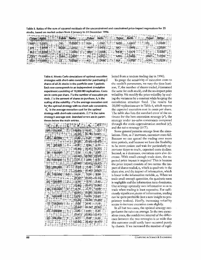
Table 5. Ratios of the sum of squared residuals of the unconstrained and constrained price-impact regressions for 25 stocks. bared on market orders from 2 lanuarv to 31 December 1996.

Table 6. Monte Carlo simulations of optimal execution strategies with short-sales constraints for purchasing 3 shares of all 25 stocks in the portfolio over Tperiods. Each row corresponds to an independent simulation experiment consisting of 10,000 IID replications. Costs are in cents per share. Tis the number of execution periods. i is the amount of shares to purchase. k, i s the scaling of the volatility. seis the average execution cost fo: the optimal strategy with no short-sale constraints.

strategy with short-sale constraints. I I T i s the naive strategy’s average cost. Standard errors are in parentheses below the main entries.

I, i s the average execution cost for the optimal

lected from a random trading day in 1996). To gauge the sensitivity of execution costs to

the model’s parameters, we vary the time horizon, T, the nuinher of shares traded, S (assumed the same for each stock), and the no-impact price volatility. We modify the pricc volatility by scaling the variances by a constant while keeping the correlation Struchlre fixed. The results for 10,000 replications are in Table 6, which reports the expected execution cost in cents per share. The table also lists the standard error of the es- tiinate for the best-execution strategy ($7, the strategy under no-sales constraints computed through the static-approximation method ($3, and the naive strategy (SIT).

Some general patterns enierge from the siniu- lations. First, as Tincreases, execution costs fall. Because we can spread the trading over more time periods, and because we have tlie flexibility to be more paticnt and wait for particularly op- portnne times to trade, expected costs decline. Second, as S decreases, cxecution costs also decrease. With small-enough trade sizes, the expected price impact is negative! This is because the price impact consists of two terms: the impact of shares traded, E,, which is quadratic in the share size, and the impact of information, which is linear in the information variable, .ep When we trade small-enough quantities, the qusdratic term is negligible and the information term dominates. Our strategy optimally uscs information so as to trade when trading is least expensive. For sufficiently significant pieces of information, trading can be quite profitable (not a uew insight to proprietary traders). Finally, increasing volatility seems to increase execution costs slightly.

In all but two cases, the optimal strategy out- performs the naivc on average. In the two anorn- alous cases, the confidence interval of the difference bctwecn the two strategies is so wide that this outcome could easily have occurred pmely by chance. If we increased the number of repli-


cations to 100,000, these two anonlalies would n o doubt disappear.

Another anotnalous result is t h a t for some simulations, t h e constraincd strategy's execotion cost is less than the uticonstraiticd strategy's cost. Although t h e point estimates are indeed reversed in these cases, t h e sampling variation is so great (consider their standard errors) that tnakitig accurate inferences about their relative magnimdes is difficult. Indeed, the differences arc not stat is- tically significant. For thc cases we eonsidcr, the no-sales constraint seems to have relatively lit- tle impact o n the hest-execution strategy's performance, except in cases wi th negative execu- t ion costs. To achieve negative execution costs, the no-sales constraints niust he violated, so imposing them increases the costs dramatically.

Of course, these conclusions are highly portfo- l io- and time-period-specific. Similar analyses should he coiiclucted case by case to determine the value added by the best-execution strategy in a given context.

he remaining challenge i s to integrate these best-execution suatcgies directly into the investment process, which re- T quires solving the portfolio optimiza-

tion problem subject to transactions costs. This i s a formidable challenge t h a t i s both theoretically and cornputationally intensive, and we plan to turn to these problem in fuhlre research. 51

Acknowledgments This research is part of the MIT laboratory for Financial Engineering's Transactions Costs Project. We are grate- ful to Investment Technology Group, the National Sci- ence Foundation (Grants DMI-9610486 and SBR- 9709976), and the sponsors of the LFE for financial support. We thank Dave Cushing, Chris Darnell, Robert Ferstenberg, Rohit D'Souza, john Heaton, Leonid Kogan, Bruce lehmann, Greg Peterson, liang Wang, and seminar participants at Columbia, Harvard, the London Business School, MIT; Northwestern, the NYSE Conference on Best Execution, the Society of Quantitative Analysts, and Yale for heipful comments and discussion.

References I , T. Loeb, "Trading Cost: The Critical Link between Investment In-

formation and Results," Finnonool Analysts I., Vol. 39, 1983, pp. 3944.

2. L. Chan and I. Lakanirhak, "The Behavior of Stock Pricer around InititutionalTrader." 1. Finnonce, Val. 50. 1995, pp. 1147-11 74.

3 . 0. Keim and A. Madhavan, "Analomy of the Trading Procerr: Empirical Evidence on the Behavior of Institutional Traders," I.

Finnancial€conamicr, Vol. 37, No. 3, Mar. 11195, pp. 371-398.

4. D. Keim and A. Madhavan, "The Upstair5 Market for Large-Block Transactions: Analysis and Measurement of Price Effects; Rev. RnonciolStudies, Vol. 9, No. 1 , Spring 1996, pp. 1-36.

5. D. Keim and A. Madhavan, "Execution Costs and Investment Performance: An Empirical Analysis of Institutional Equity Trades." working paper, School of Burinerr Administration, Univ. of Southern California, Lor Angeles, 1995.

6. D. Bert6imas and A. Lo, "Optimal Control ai Execution Costs," I. Finonciol Morkets, Vol. 1 , No. 1 , 30 Apr. 1998, pp. 1-50,

7. A. Shleifer, "Do Demand Culver for Stocks Slope Downy 1. FI- nonce, Vol. 41, 1986, pp. 579-590.

8. A. Lo and C. MscKinlay, "When Are Contrarian Profits Due to Stock Market Overreaction?" Rev. FlnnonWI Studies, Val. 3, No. 2, Summer 1990, pp. 175-205.

9. L. Birinyi, Whot Doer inrtitutional iiodimj Cost! 8irinyi Associates, Greenwich, Cann., 1995.

10. D. Leinweber, "Using Inlormation from Trading in Trading and Portfolio Management," fxecu[im ieihnlquei, True Trodiny Costs, andthe MicrortructureolMarkerr. K. Sherrerd, ed., ai io^. far ln- vestment Management and Research, Charlotterville, Va., 1993.

1 1 . D. Leinweber, "Careful Structuring Reins in Transaction Costs." Pensions ondinveitmentr, 25 iuly 1994, p. 19.

12. A. Perold, "The Implementation Shortfall: Paper v e r i ~ s Reality," 1. Portfolio Monoyernent, Vol. 14, No. 3, Spring 1988, pp. 4-11,

13. D. Bertrekar, Dynamic Programming ond Optimal Control, Val. i, Athena Scientific, Belmont, Mars., 1995.

Dimitris Bertsimas is the Boeing Professor of Opera- tions Research a t the MIT Sloan School of Manage- ment. He studies the theory and practice of optimization, as well as petformance, analysis, and control of large-scale stochastic systems. He received his PhD in operations research and applied mathematics from MiT. Contact him at the MIT Sloan School of Manage- ment and Operations Research Center, Massachusetts inst. of Technology, E53-363, Cambridge, MA 02142- 1347: [email protected].

Paul Hummel is a portfolio strategist a t Long Term Cap- ital Management, His responsibilities include trading in risk arbitrage and special situations; designing automated spread-trading, volume-weighted-average-price, and options-hedging strategies; and research support for short-term, high-frequency trading strategies. He received his MS in mechanical engineering from Cornell University and his MEA from the MIT Sloan School of Management. Contact him at Portfolio Strategist, Long Term Capital Management, One E. Weaver St., Creen- wich, CT 06831; [email protected].

Andrew W. Lo's biography appears on p, 23

NOVEMBER/DECEMBER 1999 53

mailto:[email protected]

mailto:[email protected]

optimal control of execution costs for portfolios

Documents