optimal design of regional wastewater pipelines and...

Optimal Design of Regional WastewaterPipelines and Treatment Plant Systems

Noam Brand, Avi Ostfeld*

ABSTRACT: This manuscript describes the application of a genetic

algorithm model for the optimal design of regional wastewater systems

comprised of transmission gravitational and pumping sewer pipelines,

decentralized treatment plants, and end users of reclaimed wastewater. The

algorithm seeks the diameter size of the designed pipelines and their flow

distribution simultaneously, the number of treatment plants and their size

and location, the pump power, and the required excavation work. The

model capabilities are demonstrated through a simplified example

application using base runs and sensitivity analyses. Scaling of the

proposed methodology to real life wastewater collection and treatment

plants design problems needs further testing and developments. The model

is coded in MATLAB using the GATOOL toolbox and is available from

the authors. Water Environ. Res., 83, 53 (2011).

KEYWORDS: optimization, wastewater, system.

doi:10.2175/106143010X12780288628219

Introduction

The subject of wastewater pipelines and treatment plants

systems optimization is an emerging discipline. Most of the

modeling optimization efforts, to date, concentrated on either the

transmission/sewer pipeline system or the treatment plant.

When designing a regional wastewater pipeline and treatment

plant system that connects cities to treatment plants, engineers are

facing the problem of wastewater links design and operation and

how the treated wastewater from the treatment plants will be

transported to a main concentration point for centralized

transmission. An example of such a system is shown in Figure 1.

The central collection point in Figure 1 represents a regional

mutual disposal/central transmission site. Treatment plants 1 to 3

are characterized through their cost as a function of their required

treated flow. Water quality explicit considerations are not

incorporated in this study. Only flow that needs to be transmitted

and treated is accounted for.

Searching for the best pipeline diameter links and pumping

power for such systems through enumeration is an exhaustive

process. On the other hand, exploring only a limited number of

alternatives substantially reduces the likelihood of finding an

optimal solution. Thus, an efficient search technique is required.

There are almost no optimization models that incorporate the

wastewater sources, pipeline/transmission network, treatment

plants, and end disposals/users, in a single framework. The

objective of this study is to develop and demonstrate a model of

this type.

The developed model in this work addresses a single objective

of minimizing the capital and operational costs of a wastewater

treatment plant (WWTP) system by using a genetic algorithm

(GA) framework. Through a simplified example application, the

potential of the proposed model for solving the design problem of

sizing wastewater collection and treatment plants systems is

demonstrated.

Literature Review

A literature review on wastewater optimization models divided

into optimization models for sewer networks, treatment plants,

and the entire system, is presented herein.

Sewer Networks Optimization. Early studies on sewer

networks optimization used dynamic programming for the least

cost design of sewer systems (Dajani et al., 1977; Nzewi et al.,

1985; Walters, 1985). Dajani et al. (1977) used separable convex,

dynamic, and geometric programming for optimizing the layout

and capacity of a sewer system. Nzewi et al. (1985) developed a

heuristic search methodology coupled with discrete dynamic

programming for the least cost design of sewer networks. Walters

(1985) used dynamic programming for the least cost design of

sewer networks considering the sewers diameters, nodes layout,

diameters, and slopes as decision variables. Abraham et al. (1998)

used deterministic dynamic programming for identifying suitable

sewer rehabilitation techniques during the planning horizon of a

sewer system. deMonsabert et al. (1999) used integer program-

ming to optimize sewer rehabilitation schedules for minimizing

the costs of repairs and the inflow and infiltration associated with

sewer pipeline and manhole defects. Diogo and Graveto (2006)

extended previous studies by presenting a multi-level dynamic

programming model for the optimal deterministic selection of

sewer pumping stations, intermediate manholes, pipe sections, and

pipeline installation depth. The deterministic model was extended

further to incorporate uncertainty through the implementation of a

simulated annealing scheme. Weng and Liaw (2007) used mixed

integer programming coupled with a screening bounded implicit

enumeration algorithm for sewer network optimization, demon-

strating a saving of approximately 12% compared with using

traditional sewer design approaches. Breysse et al. (2007)

developed a technical and economic performance index for asset

aging and maintenance of sewer systems. The index was

demonstrated for optimal inspection, maintenance, and rehabili-

tation strategies of sewer networks. Chang and Hernandez (2008)

outlined several schemes for sewer system optimal expansion

under uncertainty. The methodology included deterministic least-

cost optimization modeling algorithms, which further incorporat-

Technion–Israel Institute of Technology, Haifa, Israel.

* Faculty of Civil and Environmental Engineering, Technion–IsraelInstitute of Technology, Haifa 32000, Israel; e-mail: [email protected].

January 2011 53

ed uncertainty through a grey mixed integer programming model.

Ocampo-Martinez et al. (2008) used a lexicographic optimization

approach in a model predictive control framework for the

prioritization of multi-objective cost functions of sewer networks.

The model effectiveness was demonstrated on a portion of the

Barcelona sewer system.

Treatment Plant Optimization and Control. Numerous

wastewater management studies related to optimizing the design,

calibration, operation, and control of treatment plants were

published in the research literature in the last 3 decades. A

review of selected recent modeling efforts, mostly relevant for

extending the capabilities of the current study, is provided below.

Chang et al. (2001) developed a methodology for industrial

WWTP control by linking a genetic algorithm with a neural

network model for addressing the uncertainty involved in the

operation of WWTP operation. The developed methodology uses

a generic hybrid methodology, which can be adapted to other

WWTP problems. Chen et al. (2001, 2003) used a similar

framework as that of Chang et al. (2001), yet with adding a fuzzy

logic layer for assessing the control of the treatment plants. Chen

and Chang (2007) proposed a special rule-based extraction

analysis for optimal design of an integrated neural-fuzzy process

controller and rules for screening out inappropriate fuzzy

operators. The rule was demonstrated using an aerated submerged

biofilm wastewater treatment process. Chen et al. (2007)

developed a hybrid artificial neural network model coupled with

a genetic algorithm for predicting the effluent water quality data

of a treatment plant. Zeng et al. (2007) developed a model for the

selection of wastewater treatment alternatives based on the

application of an analytic hierarchy process coupled with grey

relational analysis. Beraud et al. (2007) constructed a multi-

objective genetic algorithm optimization model using the

Benchmark Simulation Model 1 (Copp, 2002) for trading off

effluent quality versus energy consumption of a treatment plant.

Holenda et al. (2007) applied a genetic algorithm to optimize the

aerobic and anoxic conditions required for nitrogen removal of a

treatment plant. Pollution loads and energy consumptions were

minimized, showing a substantial improvement over previous

applied control methodologies. Gupta and Shrivastava (2008)

developed a treatment plant reliability-constrained optimal design

model by linking a genetic algorithm with Monte Carlo

simulations. The objective function minimized the cost subject

to design- and reliability-based performance constraints. Saveyna

et al. (2008) used a quadratic model for the assessment of the

relative importance of different sludge and polyelectrolyte

variables with regard to sludge pressure dewatering.

System Optimization. Optimization of complete wastewater

systems started to receive attention only recently. This is both

because of the understanding that optimizing the sewer network

and the treatment plant separately can result in sub-optimal

solutions, and as the use of generic heuristic optimization search

techniques such as genetic algorithms (Goldberg, 1989; Holland,

1975) are becoming more common in engineering practices,

allowing a holistic representation of the system for optimizing its

performance.

Vollertsen et al. (2002) linked a model for in-sewer microbial

process simulations with treatment plant design. The model was

implemented for optimizing the layout of a sewer system for

meeting the requirements of various treatment plant treatment

scenarios. Butler and Schutze (2005) developed a coupled

simulation and control methodology for integrated real-time control

strategies of urban wastewater systems. Leitao et al. (2005)

suggested a decision support tool based on geographic information

systems and two greedy algorithms for optimal planning of regional

wastewater systems. Joksimovic et al. (2008) presented an

integrated decision support framework for optimization of

treatment and distribution aspects of water reuse and end-users

selection. Lim et al. (2008) minimized the capital and operational

costs associated with a total wastewater treatment network system,

including distributed and terminal water treatment plants, using

life-cycle assessment and life-cycle costing.

The models cited in the literature review deal with optimizing

portions of a wastewater and treatment plant system. None of

them address the problem of optimizing the entire system, with an

explicit description of the system hydraulics, sewer flows as

decision variables, excavation costs, and pipelines and pumping

system costs, as this study is proposing.

Model Formulation

In this section, the objective function components, constraints,

and decision variables are outlined. The selected model coeffi-

cients herein are empirical, based on Dekel (2006) and Friedler

and Pisanty (2006). Friedler and Pisanty (2006) derived cost

functions expressing the effects of design flow and treatment level

on construction costs, through the analysis of 55 municipal

WWTPs in Israel (secondary, advanced secondary, and advanced

treatment). Dekel (2006) is an Israeli price list database

specialized in civilian engineering and construction. Its data set

is established according to results of tenders of governmental

offices, authorities, and private bodies. The database includes

prices of sections in the fields of civil engineering, construction

works, concrete, installations, electricity, and various construction

Figure 1—Schematic layout of a regional wastewaterpipeline and treatment plant system.

Brand and Ostfeld

54 Water Environment Research, Volume 83, Number 1

materials. Other coefficients using different empirical data likely

could be adopted.

Objective Function. The objective function is the total cost

of construction (eqs 1 to 4) and operation (eq 5), comprised of the

following parts:

(1) Pumping pipeline construction cost:

Cpp~C1

.FRCpp int, nppð Þ~382:5 D1:455

p L ð1Þ

Where

Cpp ($) 5 pipeline construction cost;

C1 ($/year) 5 annual pumping pipeline construc-

tion cost;

FRCpp (int, npp) 5 annual pipe cost return coefficient,

which is equal to int (1 + int)npp / [(1

+ int)npp 2 1], where int 5 annual

interest, npp (years) 5 life span of

the pipeline; Dp (cm) 5 pipeline

(steel) diameter for pumping line;

and L (km) 5 pipeline length.

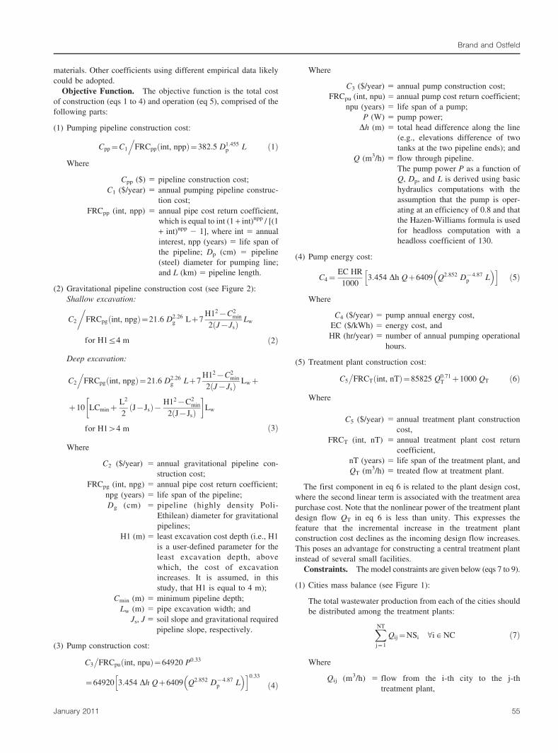
(2) Gravitational pipeline construction cost (see Figure 2):

Shallow excavation:

C2

�FRCpg int, npgð Þ~21:6 D2:26

g Lz7H12{C2

min

2 J{Jsð Þ Lw

for H1ƒ4 m ð2Þ

(2) Deep excavation:

C2

.FRCpg int, npgð Þ~21:6 D2:26

g Lz7H12{C2

min

2 J{Jsð Þ Lwz

z10 LCminzL2

2J{Jsð Þ{ H12{C2

min

2 J{Jsð Þ

� �Lw

for H1w4 m ð3Þ

Where

C2 ($/year) 5 annual gravitational pipeline con-

struction cost;

FRCpg (int, npg) 5 annual pipe cost return coefficient;

npg (years) 5 life span of the pipeline;

Dg (cm) 5 pipeline (highly density Poli-

Ethilean) diameter for gravitational

pipelines;

H1 (m) 5 least excavation cost depth (i.e., H1

is a user-defined parameter for the

least excavation depth, above

which, the cost of excavation

increases. It is assumed, in this

study, that H1 is equal to 4 m);

Cmin (m) 5 minimum pipeline depth;

Lw (m) 5 pipe excavation width; and

Js, J 5 soil slope and gravitational required

pipeline slope, respectively.

(3) Pump construction cost:

C3

�FRCpu int, npuð Þ~64920 P0:33

~64920 3:454 Dh Qz6409 Q2:852 D{4:87p L

� �h i0:33

ð4Þ

Where

C3 ($/year) 5 annual pump construction cost;

FRCpu (int, npu) 5 annual pump cost return coefficient;

npu (years) 5 life span of a pump;

P (W) 5 pump power;

Dh (m) 5 total head difference along the line

(e.g., elevations difference of two

tanks at the two pipeline ends); and

Q (m3/h) 5 flow through pipeline.

The pump power P as a function of

Q, Dp, and L is derived using basic

hydraulics computations with the

assumption that the pump is oper-

ating at an efficiency of 0.8 and that

the Hazen-Williams formula is used

for headloss computation with a

headloss coefficient of 130.

(4) Pump energy cost:

C4~EC HR

10003:454 Dh Qz6409 Q2:852 D{4:87

p L� �h i

ð5Þ

Where

C4 ($/year) 5 pump annual energy cost,

EC ($/kWh) 5 energy cost, and

HR (hr/year) 5 number of annual pumping operational

hours.

(5) Treatment plant construction cost:

C5

�FRCT int, nTð Þ~85825 Q0:71

T z1000 QT ð6Þ

Where

C5 ($/year) 5 annual treatment plant construction

cost,

FRCT (int, nT) 5 annual treatment plant cost return

coefficient,

nT (years) 5 life span of the treatment plant, and

QT (m3/h) 5 treated flow at treatment plant.

The first component in eq 6 is related to the plant design cost,

where the second linear term is associated with the treatment area

purchase cost. Note that the nonlinear power of the treatment plant

design flow QT in eq 6 is less than unity. This expresses the

feature that the incremental increase in the treatment plant

construction cost declines as the incoming design flow increases.

This poses an advantage for constructing a central treatment plant

instead of several small facilities.

Constraints. The model constraints are given below (eqs 7 to 9).

(1) Cities mass balance (see Figure 1):

(1) The total wastewater production from each of the cities should

be distributed among the treatment plants:

XNT

j~1

Qij~NSi Vi [ NC ð7Þ

Where

Qij (m3/h) 5 flow from the i-th city to the j-th

treatment plant,

Brand and Ostfeld

January 2011 55

NSi (m3/h) 5 total wastewater production of the i-th

city,

NC 5 number of cities, and

NT 5 number of treatment plants.

(2) Treatment plant mass balance:

(2) The total incoming wastewater to a treatment plant should be

equal to the total treated flow effluents, as follows:

XNC

i~1

Qij~TSj Vj [ NT ð8Þ

Where

TSj (m3/h) 5 total effluents outlet from the j-th

treatment plant.

(3) Gravitational min-max flow:

(3) The Manning’s equation for flow in a non-full cross-section of

80% of the pipeline diameter is used for gravitational

pipelines. This leads to an average cross-section velocity, Vg

(m/s), as in eq 9, using a Manning’s headloss coefficient of

0.013.

Vg~1:615 D0:667g J0:5 ð9Þ

Minimum and maximum velocity requirements of 0.6 (m/s) and

2.5 (m/s), respectively, are imposed to avoid particles accumu-

lation and to protect the pipeline.

Decision Variables. The decision variables are the vectors of

flows (Q), diameters (D), and required gravitational pipeline slopes

(J). The flows (Q) and the required gravitational pipeline slopes (J)

are continuous decision variables. The vector of diameter D is

discrete in reality, but, in this study, is treated as continuous. This is

a model simplification justified by the assumption that the influence

on the objective function value, resulting from choosing the nearest

appropriate commercial pipe diameter, or two pipelines in series,

which generate the same hydraulic headloss as the model diameter

selection, is small. Such a simplification was used previously (e.g.,

Fujiwara and Khang, 1990) for distribution system optimization

and is made to ease the model solution scheme. However, it is not a

necessity, as a genetic algorithm is used. No constraints are imposed

on the required pump capacities.

Complete Model. The complete mathematical formulation of

the model is as follows:

MinimizeQ, D, J§0

X5

k~1

Ck Q, D, Jð Þ ð10Þ

Which is subject to the following:

XNT

j~1

Qij~NSi Vi [ NC ð11Þ

XNC

i~1

Qij~TSj Vj [ NT ð12Þ

0:6ƒVgƒ2:5 Vg [ G ð13Þ

Where

Ck 5 k-th component of the objective function total

annual cost (e.g., C1 5 vector of all pumping

pipeline construction costs); and

G 5 set of all gravitational pipelines.

Solution SchemeA MATLAB code using the genetic algorithm toolbox

GATOOL based on Chipperfield et al. (1994) was implemented

Figure 2—Schematic of a gravitational pipeline layout.

Brand and Ostfeld


for solving the model outlined in eqs 10 to 13. Although other

genetic algorithm tools could have been selected (e.g., optiGA,

2002), the MATLAB environment was chosen, as it provides

convenient access to additional modeling and built-in simulation

software especially suited for control problems. It should be noted

that other evolutionary computational schemes, such as Ant

Colony (Dorigo et al., 1996), likely could be implemented.

Genetic algorithms (Goldberg, 1989; Holland, 1975) are

heuristic combinatorial search techniques that imitate the

mechanics of natural selection and natural genetics of Darwin’s

evolution principle. The basic idea is to simulate the natural

evolution mechanisms of chromosomes (represented by string

structures), involving selection, crossover, and mutation. This is

accomplished by creating a random search technique, which

combines survival of the fittest among string structures with a

randomized information exchange. As genetic algorithms are

already very well-known schemes for heuristic optimization, the

reader is refereed to any genetic algorithm text book (e.g.,

Goldberg, 1989) for further technical information.

Example Application

The layout of an example application is shown in Figure 3. The

system is comprised of two cities connected through four optional

gravitational and pumping pipelines to three possible treatment

plants, which are further linked using three gravitational pipelines

to a central collection point. The problem base run parameters are

provided in Table 1.

The example application incorporates the following subsec-

tions:

(1) Genetic algorithm base run and genetic algorithm parameters

statistics sensitivity runs,

(2) Results for the best base-run-obtained solution, and

(3) Problem-oriented sensitivity runs.

Genetic Algorithm Base Run and Parameters StatisticsSensitivity Runs. Figures 4 and 5 summarize the data and

results of statistics of 100 model runs for each of 10 cases—1 base

run and 9 genetic algorithm additional parameter sensitivities (i.e.,

a total of 1000 model repetition trials) using the MATLAB genetic

algorithm toolbox GATOOL on a Dual Core 2.26 GHz, 4GB

RAM PC.

The following genetic algorithm base run parameters were

used:

N Population size of 100—100 individuals in each generation;

N Fitness scaling of type rank—scales the population individ-

uals according to their rank within the population sorted scores;

N Selection method of type stochastic uniform—selects parents

for reproduction using a line in which each parent corresponds

to a section of a line of a length proportional to its expectation;

N Elite count of 2—specifies the number of best individuals in

each generation that move unchanged to the next generation;

N Crossover fraction of 0.8—defines the next generation

fraction produced by crossover;

N Crossover of type scattered—uses a random binary vector for

gene combinations of individual parents for reproduction;

N Mutation of type Gaussian, with a scale of 2 and a shrink of

1—generates a random number for mutation for each individual

string using a Gaussian distribution centered on zero. The scale

of 2 specifics a standard deviation of 2 for the first generation,

which shrinks linearly to zero at the last generation with a

shrink parameter of 1; and

N Stopping criteria—the foremost to occur among the use of a

maximum of 2000 generations or a computational time

exceeding 20 seconds with no model improvement.

In GA-SA1 (genetic algorithm sensitivity analysis 1), the

selection method was altered to tournament of size 2 (i.e., a

tournament between two randomly selected individuals, from

which the better is chosen as a parent); in GA-SA2, a roulette

wheel was applied for selection (i.e., using a roulette wheel for

parents selection, with the roulette area partitioned into segments,

where each segment is proportional to an individual expectation

according to its fitness); in GA-SA3, the elite count was modified

to 5; in GA-SA4, the crossover fraction was altered to 0.9; in GA-

SA5 and GA-SA6, a 1-point crossover (i.e., a single crossover

location on each individual string) and 2-points crossover (i.e., 2-

points crossover locations on each individual string) were used,

respectively; in GA-SA7, the Gaussian mutation scale was altered

to 4; in GA-SA8, the population size was increased to 200; and, in

GA-SA9, the population size was modified to 200 and the

stopping criteria to a maximum of 4000 generations and a

maximum computational time of 60 seconds with no results

improvement.

The top and bottom of Figure 4 describe the genetic algorithm

data and results, respectively. Figure 4 shows that the best result

was attained for the base run for all cases in which the population

size remained unchanged (i.e., GA-SA1 to SA7). As the

population size increased, a better solution was received (i.e.,

GA-SA8, SA9). Increasing the population size and relaxing the

stopping criteria in GA-SA9 resulted in the best solution, although

Figure 3—Example application layout.

Brand and Ostfeld

January 2011 57

Table 1—Example application base run data.

Parameter Description Value (Units)

Cmin Minimum pipeline depth Assumed very close to the surface (i.e.,

approximately zero)

EC Energy cost 0.1 ($/kWh)

FRCpp (int, npp); FRCpg (int, npg) Annual cost return coefficient for pipeline

construction

0.075 (2)

FRCpu (int, npu) Annual cost return coefficient for pump

construction

0.110 (2)

FRCT(int, nT) Annual cost return coefficient for treatment plant

construction

0.072 (2)

H1 Least excavation cost depth 4 (m)

HR Number of annual pumping operation hours 8760 (h/year)

int Annual interest 7 (%)

Js Soil slope assumed zero or very close to zero

Lw Pipe excavation width pipe diameter + 0.6 (m)

L1, …, L7 Link length 1 (km)

NS1, NS2 Total wastewater production for city 1 and city

2, respectively

1000 (m3/h)

npp, npg Life span of pipeline 40 (years)

npu Life span of pump 15 (years)

nT Life span of treatment plant 50 (years)

Vg, min ; Vg, max Minimum and maximum gravitational pipeline

velocities, respectively

0.6, 2.5 (m/s)

Dh Total head difference along a line 10 (m)

Figure 4—Genetic algorithm sensitivity analysis.

Brand and Ostfeld


with minor improvement (i.e., 1 818 468 $/year in GA-SA8

compared with 1 816 130 $/year in GA-SA9). The best solution

obtained in GA-SA9 used the maximum number of function

fitness evaluations and the highest computational price of 0.308

(i.e., ratio of average number of function fitness evaluations to

convergence to average solution).

Figure 5 scales the best solution acquired in GA-SA9 to all

other cases and the corresponding computational price. Figure 5

shows that the worst result among all cases (i.e., SA-GA5) has the

lowest computational price of 0.059. It is relatively distant from

the best solution (i.e., GA-SA9) by approximately 3.6%.

Figure 6 shows a typical progression of the genetic algorithm; the

first feasible solution is obtained at generation 66 at an annual cost of

approximately 1.9 3 106 ($/year); the algorithm then progresses in a

‘‘stair-like’’ manner, with the best attained solution of approximately

1.86 3 106 ($/year) received after 500 generations.

Detailed Base Run Results. Figure 7 presents the best base-

run-obtained results, and Table 2 presents detailed results for the

best base run and three problem-oriented sensitivity analyses runs.

Figure 7 shows that gravitational pipeline 1 and pumping pipeline

3 were selected to transmit the cities’ wastewater production to

treatment plant 1, and gravitational pipeline 5 was selected to

Figure 5—Genetic algorithm runs comparison.

Figure 6—Typical progression of the genetic algorithm.

Brand and Ostfeld

January 2011 59

transmit the cities’ wastewater production to the central collection

point. To guarantee a minimum pipeline diameter, links were

excluded during the solution process (i.e., assigned a zero flow) if

their capacity was less than 10% of the entire cities’ wastewater

production. Using this heuristics links 2, 4, 6, and 7, and, as a

result, treatment plants 2 and 3 were excluded from the final

solution. It should be noted that the 10% figure for pipes

elimination is heuristic for simplification purposes (i.e., similar to

treating pipe diameters as continuous instead of discrete

variables). Incorporating a decision of ‘‘elimination’’ is binary

(i.e., 0 or 1) and can be used in principle as a genetic algorithm is

used.

The best base run solution obtained was a total cost of

1 821 248 ($/year), with most of its portion (83.3%) devoted to

the treatment plant construction cost, 15.1% for the pumping

pipeline, and only 1.6% for the gravitational transmission. As the

treatment plant construction cost dominates the solution costs,

only one treatment plant was selected. The velocity (2.3 m/s) at

gravitational pipeline 5 is close to the maximum allowable

gravitational pipeline velocity of 2.5 m/s.

Problem-Oriented Sensitivity Analysis Runs. Four sensi-

tivity analysis runs aimed at testing the model solution behavior to

modifications made in the problem data or the constraints, as

compared with the base run results, are explored herein.

In sensitivity analysis 1 (SA1), each city’s wastewater

production was doubled (i.e., 2000 m3/h compared with

1000 m3/h at the base run). As a result (Table 2), the total system

cost was increased to 2 964 332 ($/year) (85.5% for the treatment

plant cost, 12.6% for the pumping pipeline, and 1.9% for the

gravitational transmission). The results of SA1 show that the

entire system capacity was increased, and the system layout (i.e.,

the selection of pipelines 1, 3, and 5, and treatment plant 1)

remained unchanged; the gravitational pipelines 1 and 3 diameters

were increased to 60 and 82 cm, respectively (compared with 43

and 58 cm, respectively, at the base run); the pumping pipeline

diameter was increased to 90 cm (75 cm at the base run), and the

pumping power was increased to 74 kW (36 kW at the base run).

The SA1 results demonstrate, as in the base run, the dominance of

the treatment plant cost; thus, the model selects to increase

capacity, yet not to alter the base run model layout.

In sensitivity analysis 2 (SA2), pumping pipeline 3 is excluded

(i.e., only pipelines 1, 2, 4, 5, 6, and 7 are considered). The model

selects four gravitational pipelines—1, 4, 5, and 7, all with the

same diameter of 43 cm at a slope of 0.013, and two treatment

plants (1 and 3). The total system cost is 1 871 536 ($/year), out

of which, 97.4% is for the treatment plants cost and 2.6% is for the

pipelines. Note that the obtained cost of 1 871 536 ($/year) is an

increase over the base run solution of 1 821 248 ($/year). This is

the result of the removal of pipeline 3, which imposes an

additional constraint to the model, thus reducing the feasible

domain, which results in an increase in cost.

In sensitivity analysis 3 (SA3), the length of links 1, 3, and 5 are

increased to 20 km (1 km at the base run; i.e., the distance of

treatment plant 1 to the cities and to the central collection point is

increased substantially). As a result, pumping pipeline 2 is

selected (with the same properties as pipeline 3 in the base run),

with gravitational pipelines 4, 6, and 7, and treatment plants 2 and

3. The total system cost is increased to 2 133 444 ($/year), out of

which, 85.4% is for the treatment plants construction, 12.9% is for

the pumping pipeline, and 1.7% is for the gravitational pipelines.

In sensitivity analysis 4 (SA4), the model was run with different

annual interest rates—5 to 10% (7% at the base run). Figure 8

shows the tradeoff (i.e., the exchange) between the system’s cost

results and the annual interest rate (best solutions out of 100 trials

for each explored interest rate). Figure 8 shows that the system’s

cost increased approximately linearly as the interest rate

increased.

Figure 9 is a graphical summary of the best base run and SA1-

SA3 sensitivity runs, as described above, showing the relative

percentage in all runs of the objective function components C1,

…C5. For example, the gravitational pipeline construction relative

cost (C2) is 17% (29 181 $/year) for the base run, 33% (56 305 $/

year) for SA1, 29% (48 812 $/year) for SA2, and 21% (35 852 $/

year) for SA3.

Conclusions

A genetic algorithm model for optimizing regional wastewater

treatment systems comprised of transmission gravitational and

pumping sewer pipelines, decentralized treatment plants, and end-

users of reclaimed wastewater was developed and demonstrated.

The model was coded in MATLAB using the GATOOL toolbox,

which provides a convenient environment for genetic algorithm

analysis and further access to control simulation tools.

The model contribution to wastewater pipelines and treatment

plants systems optimization is in providing an integrated model

for optimizing a total regional wastewater treatment network

system, considering the following:

(1) An explicit formulation of the system’s hydraulics for both the

sewers and pumping pipelines;

(2) Pipeline flows as decision variables, where previous studies

optimized the system for a given flow distribution, which

Figure 7—Best base run results.

Brand and Ostfeld


substantially narrowed the feasibility domain and thus the

ability to obtain good solutions; and

(3) Possible modifications in the system’s layout, by initially

suggesting a ‘‘rich’’ layout setup and allowing the model to

select and size the most appropriate pipelines, pumps, and

treatment plants.

A simplified example application was explored for 1 base run

and 13 sensitivity analysis cases—9 for the influence of modifying

genetic algorithm parameters and 4 for altering problem-

dependent data. The genetic algorithm sensitivity results showed

the following:

(1) Convergence in all cases to the vicinity of the best obtained

solution, with a maximum relative difference of 3.6%, and

(2) That the most significant genetic algorithm parameter was the

population size.

The problem-oriented sensitivity runs produced explanatory

outcomes, showing a close-to-linear tradeoff between the system

cost and the annual interest rate. However, it should be

emphasized that the example application is a simplified

representation of reality and was meant to demonstrate a ‘‘proof

of concept’’. Extension of the proposed methodology to real-world

problems with a network of pipes and geographical constraints

will need to address issues such as the following:

(1) Different pipe materials, routes, and cross-sections;

(2) Locations of pumping stations with diverse characteristics;

(3) Storage facilities and their effects;

(4) Pipes network layout complexities;

(5) Multiple loadings;

(6) An improved representation of the cost functions and, in

particular, the treatment plant construction and operation

costs, as related to the treated wastewater quality and

geographical location; and

(7) Multi-objective optimization frameworks (e.g., reliability/risk

versus cost).

In reality, the system will be highly complex; it is anticipated

that the parameters that will be the most dominant in determining

Table 2—Best base run and sensitivity analysis detailed results.*

Component Feature BR SA1 SA2 SA3

Pipeline 1 (G) PICC ($/year); EXC ($/year) 7965; 2395 16 912; 2790 7965; 4237 NS

TC ($/year) 10360 19 702 12 203

J (2); D (cm) 0.008; 43 0.008; 60 0.013; 43

Q (m3/h); V (m/s) 1000; 1.8 2000; 2.2 1000; 2.3

Pipeline 2 (P) Q (m3/h); D (cm); P (kW) NS NS NS 1000; 75; 36

PUCC ($/year); EC ($/year);

PICC ($/year)

227 774; 31 749;

15 345

TC ($/year) 274 868

Pipeline 3 (P) Q (m3/h); D (cm); P (Kw) 1000; 75; 36 2000; 90; 74 RC NS

PUCC ($/year); EC ($/year);

PICC ($/year)

227 774; 31 749;

15 345

288 454; 64 947;

20 006

TC ($/year) 274 868 373 407

Pipeline 4 (G) PICC ($/year); EXC ($/year) NS NS 7965; 4237 10 213; 2141

TC ($/year) 12203 12 354

J (2); D (cm) 0.013; 43 0.007; 48

Q (m3/h); V (m/s) 1000; 2.3 1000; 1.8

Pipeline 5 (G) PICC ($/year); EXC ($/year) 15 664; 3157 34 260; 2343 7965; 4237 NS

TC ($/year) 18 821 36 603 12203

J (2); D (cm) 0.009; 58 0.006; 82 0.013; 43

Q (m3/h); V (m/s) 2000; 2.3 4000; 2.4 1000; 2.3

Pipeline 6 (G) PICC ($/year); EXC ($/year) NS NS NS 7553; 4196

TC ($/year) 11 749

J (2); D (cm) 0.013; 42

Q (m3/h); V (m/s) 1000; 2.2

Pipeline 7 (G) PICC ($/year); EXC ($/year) NS NS 7965; 4237 7553; 4196

TC ($/year) 12 203 11 749

J (2); D (cm) 0.013; 43 0.013; 42

Q (m3/h); V (m/s) 1000; 2.3 1000; 2.2

TP1 TC ($/year) 1 517 199 253 4619 911 362 NS

TP2 TC ($/year) NS NS NS 911 362

TP3 TC ($/year) NS NS 911 362 911 362

Total system cost

($/year)

1 821 248 296 4332 1 871 536 2 133 444

* Legend:

BR 5 base run; SA1 5 sensitivity analysis 1; Pipeline 1 (G), Pipeline 2 (P) 5 optional gravitational pipeline 1 and pumping pipeline 2,

respectively; TP1 5 treatment plant 1; PICC, EXC, TC ($/year) 5 annual pipeline construction, excavation, and total cost, respectively; J

(2) 5 pipeline slope; D (cm) 5 pipeline diameter; Q (m3/h) 5 pipeline flow; V (m/s) 5 pipeline velocity; P (kW) 5 pump power; PUCC, EC

($/year) 5 annual pump construction, and energy cost, respectively; NS 5 not selected; and RC 5 removed connection.

Brand and Ostfeld

January 2011 61

the total cost will differ as a function of the particular systems

layout, components, cost functions, and imposed loadings. As

genetic algorithms prove to be robust and reliable schemes, we

believe that such extensions are doable, yet with an anticipated

increase in computational costs.

Nomenclature

C1 ($/year) 5 annual pumping pipeline construction cost,

C2 ($/year) 5 annual gravitational pipeline construction cost,

C3 ($/year) 5 annual pump construction cost,

C4 ($/year) 5 pump annual energy cost,

C5 ($/year) 5 annual treatment plant construction cost,

Ci 5 vector of the i-th component of the objective function,

Cmin (m) 5 minimum pipeline depth,

Cpp ($) 5 pipeline construction cost,

Dg (cm) 5 pipeline (highly density Poli-Ethilean) diameter for

gravitational pipelines,

Dp (cm) 5 pipeline (steel) diameter for pumping line,

D (cm) 5 vector of pipeline diameters,

EC ($/kWh) 5 energy cost,

FRCpu (int, npu) 5 annual pump cost return coefficient,

FRCpg (int, npg), FRCpp (int, npp) 5 annual pipe cost return

coefficient,

FRCT (int, nT) 5 annual treatment plant cost return coef-

ficient,

H1 (m) 5 least excavation cost depth (assuming 4 m),

Figure 8—Tradeoff between the system cost and annual interest rate.

Figure 9—Best base run and sensitivity analysis summary results.

Brand and Ostfeld


HR (h/year) 5 number of annual pumping operation hours,

int 5 annual interest,

Js, J 5 soil slope and gravitational required pipeline slope,

respectively,

J 5 vector of required gravitational pipeline slopes,

L (km) 5 pipeline length,

Lw (m) 5 pipe excavation width,

NC 5 number of cities,

NSi (m3/h) 5 total wastewater production of the i-th city,

NT 5 number of treatment plants,

npg (years) 5 life span of the pipeline,

npp (years) 5 life span of the pipeline,

nT (years) 5 life span of the treatment plant,

npu (years) 5 life span of a pump,

O (k) 5 k-th generated population,

P (W) 5 pump power,

Q (m3/h) 5 flow through pipeline,

Q (m3/h) 5 vector of flows through pipeline,

QT (m3/h) 5 treated flow at treatment plant,

TSj (m3/h) 5 total outlet effluents of the j-th treatment plant,

Vg (m/s) 5 average cross-section velocity, and

Dh (m) 5 total head difference along the line (e.g., elevations

difference of two tanks at the two pipeline ends).

Credits

This study was supported by the Technion Grand Water

Research Institute (GWRI) (Haifa, Israel).

Submitted for publication December 8, 2009; revised manu-

script submitted July 31, 2010; accepted for publication August 9,

2010.

ReferencesAbraham, D. M.; Wirahadikusumah, R.;, Short, T. J.; Shahbahrami, S.

(1998) Optimization Modeling for Sewer Network Management. J.

Const. Eng. Manage., 124, 402–410.

Beraud, B.; Steyer, J. P.; Lemoine, C.; Latrille, E.; Manic, G.; Printemps-

Vacquier, C. (2007) Towards a Global Multi Objective Optimization

of Wastewater Treatment Plant Based on Modeling and Genetic

Algorithms. Water Sci. Technol., 56 (9), 109–116.

Breysse, D.; Vasconcelos, E.; Schoefs, F. (2007) Estimating the Capital

Cost of Wastewater System. Comput.-Aided Infrastr. Eng., 22, 462–

477.

Butler, D.; Schutze, M. (2005) Integrating Simulation Models with a View

to Optimal Control of Urban Wastewater Systems. Environ. Model.

Softw., 20, 415–426.

Chang, N. B.; Chen, W. C.; Shieh, W. K. (2001) Optimal Control of

Wastewater Treatment Plant via Integrated Neural Network and

Genetic Algorithms. Civil Eng. Environ. Syst., 18 (1), 1–17.

Chang, N. B.; Hernandez, E. A. (2008) Optimal Expansion Strategy for a

Sewer System Under Uncertainty. Environ. Model. Assess., 13, 93–

113.

Chen, H. W.; Ning, S. K.; Yu, R. F.; Hung, M. S. (2007) Optimizing the

Monitoring Strategy of Wastewater Treatment Plants by Multi-

objective Neural Networks Approach. Environ. Model. Assess., 125,

325–332.

Chen, J. C.; Chang, N. B. (2007) Mining the Fuzzy Control Rules of

Aeration in a Submerged Biofilm Wastewater Treatment Process.

Eng. Appl. Artif. Intel., 20, 959–969.

Chen, W. C.; Chang, N. B.; Chen, J. C. (2003) Rough Set-Based Hybrid

Fuzzy Neural Controller Design for Industrial Wastewater Treatment.

Water Res., 37 (1), 95–107.

Chen, W. C.; Chang, N. B.; Shieh, W. K. (2001) Advanced Hybrid Fuzzy-

Neural Controller for Industrial Wastewater Treatment. ASCE J.

Environ. Eng., 127, 1048–1059.

Chipperfield, A. J.; Fleming, P. J.; Fonseca, C. M. (1994) Genetic

Algorithm Tools for Control Systems Engineering. Proceedings of

Adaptive Computing in Engineering Design and Control, Plymouth

Engineering Design Centre, Plymouth, United Kingdom, Sept. 21–22,

128–133.

Copp, J. B. (Ed.) (2002) The Cost Simulation Benchmark-Description and

Simulator Manual; Office for Official Publications of the European

Communities: Luxembourg.

Dajani, J. S.; Hasit, Y.; Stephen, D. (1977) Mathematical Programming in

Sewer Network Design. Eng. Optimiz., 3 (1), 27–35.

Dekel (2006) Dekel Price List Data-Base. Dekel: Tel-Aviv, Israel, http://

www.dekel.co.il (accessed June 21, 2010).

deMonsabert, S.; Ong, C.; Thornton, P. (1999) An Integer Program for

Optimizing Sanitary Sewer Rehabilitation Over a Planning Horizon.

Water Environ. Res., 71, 1292–1297.

Diogo, A. F.; Graveto, V. M. (2006) Optimal Layout of Sewer Systems: A

Deterministic Versus a Stochastic Model. J. Hydraul. Eng., 132, 927–

943.

Dorigo, M.; Maniezzo, V.; Colorni, A. (1996) Ant System: Optimization

by a Colony of Cooperating Agents. IEEE Trans. Syst. Man

Cybernetics B, 26 (1), 29–41.

Friedler, E.; Pisanty, E. (2006) Effects of Design Flow and Treatment

Level on Construction and Operation Costs of Municipal Wastewater

Treatment Plants and Their Implications on Policy Making. Water

Res., 40, 3751–3758.

Fujiwara, O.; Khang, D. B. (1990) A Two-Phase Decomposition Method

for Optimal Design of Looped Water Distribution Networks. Water

Resour. Res., 26, 539–549.

Goldberg, D. E. (1989) Genetic Algorithms in Search, Optimization, and

Machine Learning; Addison-Wesley: New York.

Gupta, A. K.; Shrivastava, R. K. (2008) Optimal Design of Water

Treatment Plant Under Uncertainty Using Genetic Algorithm.

Environ. Prog., 27 (1), 91–97.

Holenda, B.; Domokos, E.; Redey, A.; Fazakas, J. (2007) Aeration

Optimization of a Wastewater Treatment Plant Using Genetic

Algorithm. Optimal Control Applic. Methods, 28 (3), 191–208.

Holland, J. H. (1975) Adaptation in Natural and Artificial Systems; The

University of Michigan Press: Ann Arbor, Michigan.

Joksimovic, D.; Savic, D. A.; Walters, G. A.; Bixio, D.; Katsoufidou, K.;

Yiantsios, S. G. (2008) Development and Validation of System

Design Principles for Water Reuse Systems. Desalination, 218, 142–

153.

Leitao, J. P.; Matos, J. S.; Goncalves, A. B.; Matos, J. L. (2005)

Contribution of Geographic Information Systems and Location

Models to Planning of Wastewater Systems. Water Sci. Technol.,

52 (3), 1–8.

Lim, S. R.; Park, D.; Park, J. M. (2008) Environmental and Economic

Feasibility Study of a Total Wastewater Treatment Network System.

J. Environ. Manage., 88, 564–575.

Nzewi, E. U.; Gray, D. D.; Houck, M. H. (1985) Optimal Design Program

for Gravity Sanitary Sewers. Civil Eng. Environ. Syst., 2 (3), 132–

141.

Ocampo-Martinez, C.; Ingimundarson, A.; Puig, V.; Quevedo, J. (2008)

Objective Prioritization Sing Lexicographic Minimizers for MPC of

Sewer Networks. IEEE Trans. Control Syst. Technol., 16 (1), 113–

121.

optiGA (2002) ActiveX Control for Genetic Algorithms. optiGA: Haifa,

Israel, http://www.optiwater.com (accessed June 21, 2010).

Saveyna, H.; Curversa, D.; Thasb, O.; der Meerena, P. V. (2008)

Optimization of Sewage Sludge Conditioning and Pressure Dewater-

ing by Statistical Modelling. Water Res., 42, 1061–1074.

Vollertsen, J.; Hvitved-Jacobsen, T.; Ujang, Z.; Talib, S. A. (2002)

Integrated Design of Sewers and Wastewater Treatment Plants. Water

Sci. Technol., 46 (9), 11–20.

Brand and Ostfeld

January 2011 63

Walters, G. A. (1985) The Design of the Optimal Layout for a Sewer

Network. Eng. Optimiz., 9 (1), 37–50.

Weng, H. T.; Liaw, S. L. (2007) An Optimization Model for Urban Sewer

System Hydraulic Design. J. Chinese Inst. Eng., 30 (1), 31–42.

Zeng, G. M.; Jiang, R.; Huang, G. H.; Xu, M.; Li, J. B. (2007)

Optimization of Wastewater Treatment Alternative Selection by

Hierarchy Grey Relational Analysis. J. Environ. Manage., 82, 250–

259.

Brand and Ostfeld


optimal design of regional wastewater pipelines and...

Documents