optimal detection with imperfect channel estimation for...
TRANSCRIPT

Optimal Detection with Imperfect ChannelEstimation for Wireless Communications
This thesis is submitted in partial fulfilment of the requirements for
Doctor of Philosophy (Ph.D.)
Junruo Zhang
Communications Research Group
Department of Electronics
University of York
September 2009

Abstract
In communication systems transmitting data through unknown fading channels, tradi-
tional detection techniques are based on channel estimation (e.g., by using pilot signals),
and then treating the estimates as perfect in a minimum distance detector. In this thesis,
we derive and investigate an optimal detector that does not estimate the channel explicitly
but jointly processes the received pilot and data symbols torecover the data. This optimal
detector outperforms the traditional detectors (mismatched detectors). In order to approx-
imate correlated fading channels, such as fast fading channels and frequency-selective
fading channels, basis expansion models (BEMs) are used due to high accuracy and low
complexity.
There are various BEMs used to represent the time-variant channels, such as
Karhunen-Loeve (KL) functions, discrete prolate spheroidal (DPS) functions, general-
ized complex exponential (GCE) functions, B-splines (BS), andthe others. We derive the
mean square error (MSE) of a generic BEM-based linear channelestimator with perfect
or imperfect knowledge of the Doppler spread in time-variant channels. We compare the
performance and complexity of minimum mean square error (MMSE) and maximum like-
lihood (ML) channel estimators using the four BEMs, for the case with perfect Doppler
spread. Although all BEM-based MMSE estimators allow achievement of the optimal
performance of the Wiener solution, the complexity of estimators using KL and DPS
BEMs is significantly higher than that of estimators using BS and GCE BEMs. We then
investigate the sensitivity of BEM-based estimators to the mismatched Doppler spread.
All the estimators are sensitive to underestimation of the Doppler spread but may be ro-
bust to overestimation. The results show that the traditional way of estimating the fading
statistics and generating the KL and DPS basis functions by using the maximum Doppler
spread will lead to a degradation of the performance. A better performance can be ob-
J. Zhang, Ph.D. Thesis, Department of Electronics, University of York
1
2009

tained by using an overestimate of the Doppler spread instead of using the maximum
Doppler spread. For this case, due to the highest robustnessand the lowest complexity,
the best practical choice of BEM is the B-splines.
We derive a general expression for optimal detection for pilot-assisted transmission
in Rayleigh fading channels with imperfect channel estimation. The optimal detector is
specified for single-input single-output (SISO) Rayleigh fading channels. The slow (time-
invariant) fading channels and fast (time-variant) fadingchannels following Jakes’ model
are considered. We use the B-splines to approximate the channel gain time variations
and compare the detection performance of the optimal detector with that of different mis-
matched detectors using ML or MMSE channel estimates. Furthermore, we investigate
the detection performance of an iterative receiver implementing the optimal detector in
the initial iteration and mismatched detectors in following iterations in a system transmit-
ting turbo-encoded data. Simulation results show that the optimal detection outperforms
the mismatched detection with ML channel estimation. However, the improvement in the
detection performance compared to the mismatched detection with the MMSE channel es-
timation is modest. We then extend the optimal detector to channels with more unknown
parameters, such as spatially correlated MIMO Rayleigh fading channels, and compare
the performance of the optimal detector with that of mismatched detectors. Simulation re-
sults show that the benefit in detection performance caused by using the optimal detector
is not affected by the spatial correlation between antennas, but becomes more significant
when the number of antennas increases.
This optimal detector is extended to the case of orthogonal frequency-division mul-
tiplexing (OFDM) signals in frequency-selective fading channels. We compare the per-
formance and complexity of this optimal detector with that of mismatched detectors us-
ing ML and MMSE channel estimates in SISO and MIMO channels. In SISO systems,
the performance of the optimal detector is close to that of the mismatched detector with
MMSE channel estimates. However, the optimal detector significantly outperforms the
mismatched detectors in MIMO channels.

Acknowledgements
I would firstly like to gratefully acknowledge my supervisorYuriy Zakharov for his help-
ful support and constant encouragement. I have learned an incredible amount from him
throughout my Ph.D. research. He has been actively interested in my work and has al-
ways been available to advise me. I am deeply benefited from his motivation, enthusiasm,
preciseness, patience, and immense knowledge in signal processing that, taken together,
make him a great mentor.
I would also like to thank all my colleagues in the Communications Research Group
for being the surrogate family during the period of my study.
This thesis is dedicated to my parents. I am forever indebtedto them for their under-
standing, endless encouragement and patience. Their unconditional love is the source of
my strength which is going to drive and motivate me forever.
Finally, I will dedicate this thesis to my grandfather. I know you are always loving and
encouraging me in heaven.
J. Zhang, Ph.D. Thesis, Department of Electronics, University of York
i
2009

Declaration
Some of the research presented in this thesis has resulted insome publications. These
publications are listed at the end of Chapter 1.
All work presented in this thesis as original is so, to the best knowledge of the author.
References and acknowledgements to other researchers have been given as appropriate.
J. Zhang, Ph.D. Thesis, Department of Electronics, University of York
ii
2009

Glossary
AWGN AdditionalWhiteGaussianNoise
BEM BasisExpansionModel
BER Bit-Error-Rate
BS B-Splines
BPSK BinaryPhaseShift Keying
CE ComplexExponential
CP Cyclic Prefix
dB Decibel
DPS DiscreteProlateSpheroidal
FEC ForwardError Correction
Hz Hertz
ICI Inter-CarrierInterference
ISI Inter-Symbol Interference
IDFT InverseDiscreteFourierTansform
GCE GeneralizedComplexExponential
KL Karhunen-Loeve
LLR Log-L ikelihoodRatio
MAP MaximumA Posteriori
MIMO Multiple-InputMultiple-Output
ML MaximumL ikelihood
MLSE MaximumL ikelihoodSequentialEstimation
MMSE M inimum MeanSquareError
MSE MeanSquareError
NSC Non-SystematicConvolutional
OFDM OrthogonalFrequencyDivision Multiplexing
PCI PerfectChannelInformation
PDF ProbabilityDensityFunction
PSAM Pilot Symbol AssistedModulation
PSK Phase-Shift Keying
QAM QuadratureAmplitudeModulation
rms root-mean-square
RSC RecursiveSystematicConvolutional
J. Zhang, Ph.D. Thesis, Department of Electronics, University of York
iii
2009

SIHO Soft-InputHard-Output
SISO Soft-InputSoft-Output
SISO Single-InputSingle-Output
SNR Signal toNoiseRatio
STBC Space-TimeBlock Codes
STTC Space-TimeTrellis Codes
SVD SingularValueDecomposition

Contents
Acknowledgements . . . . . . . . . . . . . . . . . . . . . . . . . . . . . i
Declaration . . . . . . . . . . . . . . . . . . . . . . . . . . . . . . . . . ii
Glossary . . . . . . . . . . . . . . . . . . . . . . . . . . . . . . . . . . . iii
List of Figures . . . . . . . . . . . . . . . . . . . . . . . . . . . . . . . . x
List of Tables . . . . . . . . . . . . . . . . . . . . . . . . . . . . . . . . x
1 Introduction 1
1.1 Overview . . . . . . . . . . . . . . . . . . . . . . . . . . . . . . . . . . 1
1.2 Contributions . . . . . . . . . . . . . . . . . . . . . . . . . . . . . . . . 3
1.3 Thesis Outline . . . . . . . . . . . . . . . . . . . . . . . . . . . . . . . . 4
1.4 Notations . . . . . . . . . . . . . . . . . . . . . . . . . . . . . . . . . . 6
1.5 Publication List . . . . . . . . . . . . . . . . . . . . . . . . . . . . . . . 6
2 Fundamental Techniques 9
2.1 Simulator of time-variant fading channels . . . . . . . . . . .. . . . . . 9
J. Zhang, Ph.D. Thesis, Department of Electronics, University of York
v
2009

2.1.1 The reference model and its simplifications . . . . . . . . .. . . 11
2.1.2 An improved simulation model . . . . . . . . . . . . . . . . . . . 14
2.2 Basis expansion models . . . . . . . . . . . . . . . . . . . . . . . . . . . 19
2.3 Turbo codes . . . . . . . . . . . . . . . . . . . . . . . . . . . . . . . . . 25
2.3.1 Turbo encoder . . . . . . . . . . . . . . . . . . . . . . . . . . . 25
2.3.2 Turbo decoder . . . . . . . . . . . . . . . . . . . . . . . . . . . 27
2.4 Conclusions . . . . . . . . . . . . . . . . . . . . . . . . . . . . . . . . . 33
3 Channel Estimation of Time-Varying Channels Based on Basis Expansion
Models 34
3.1 Introduction . . . . . . . . . . . . . . . . . . . . . . . . . . . . . . . . . 34
3.2 Transmission model and BEMs . . . . . . . . . . . . . . . . . . . . . . . 36
3.3 MSE of a generic linear channel estimator . . . . . . . . . . . . .. . . . 40
3.3.1 BEM-based estimator . . . . . . . . . . . . . . . . . . . . . . . . 40
3.3.2 Wiener solution . . . . . . . . . . . . . . . . . . . . . . . . . . . 42
3.4 Approach 1: Channel estimation using perfect knowledge of the Doppler
spread . . . . . . . . . . . . . . . . . . . . . . . . . . . . . . . . . . . . 43
3.4.1 BEM-based MMSE estimator . . . . . . . . . . . . . . . . . . . 43
3.4.2 BEM-based ML estimator . . . . . . . . . . . . . . . . . . . . . 46
3.5 Approach 2: Channel estimation using the maximum Dopplerspread . . . 49

3.5.1 MSE performance . . . . . . . . . . . . . . . . . . . . . . . . . 51
3.5.2 Complexity . . . . . . . . . . . . . . . . . . . . . . . . . . . . . 52
3.6 Approach 3: Channel estimation using an estimate of the Doppler spread 53
3.6.1 MSE performance . . . . . . . . . . . . . . . . . . . . . . . . . 55
3.6.2 Complexity . . . . . . . . . . . . . . . . . . . . . . . . . . . . . 58
3.7 Conclusions . . . . . . . . . . . . . . . . . . . . . . . . . . . . . . . . . 59
4 Optimal and Mismatched Detection in SISO Frequency-Flat Fading Chan-
nels with Imperfect Channel Estimation 62
4.1 Introduction . . . . . . . . . . . . . . . . . . . . . . . . . . . . . . . . . 62
4.2 Transmission model . . . . . . . . . . . . . . . . . . . . . . . . . . . . . 64
4.3 Generic optimal detection . . . . . . . . . . . . . . . . . . . . . . . . .. 65
4.4 Generic mismatched detection . . . . . . . . . . . . . . . . . . . . . .. 67
4.5 Optimal and mismatched detection in time invariant SISOchannels . . . . 69
4.6 Optimal and mismatched detection in SISO time variant channels . . . . . 70
4.6.1 Transmission model . . . . . . . . . . . . . . . . . . . . . . . . 70
4.6.2 Optimal detection . . . . . . . . . . . . . . . . . . . . . . . . . . 72
4.6.3 Mismatched detection . . . . . . . . . . . . . . . . . . . . . . . 73
4.6.4 Iterative receivers . . . . . . . . . . . . . . . . . . . . . . . . . . 74
4.7 Simulation results . . . . . . . . . . . . . . . . . . . . . . . . . . . . . . 77

4.8 Conclusions . . . . . . . . . . . . . . . . . . . . . . . . . . . . . . . . . 84
5 Optimal and Mismatched Detection in MIMO Frequency-Flat Fading Chan-
nels with Imperfect Channel Estimation 88
5.1 Introduction . . . . . . . . . . . . . . . . . . . . . . . . . . . . . . . . . 89
5.2 Optimal and mismatched detection in MIMO time invariantchannels . . . 90
5.2.1 Optimal detector . . . . . . . . . . . . . . . . . . . . . . . . . . 91
5.2.2 Mismatched detectors . . . . . . . . . . . . . . . . . . . . . . . 91
5.3 Optimal and mismatched detection in MIMO time variant channels . . . . 92
5.3.1 Transmission Model . . . . . . . . . . . . . . . . . . . . . . . . 92
5.3.2 Optimal detection . . . . . . . . . . . . . . . . . . . . . . . . . . 95
5.3.3 Mismatched detection . . . . . . . . . . . . . . . . . . . . . . . 96
5.4 The equivalence between the optimal detector and the mismatched detec-
tor with MMSE channel estimates in SIMO channels with PSK modulation 97
5.4.1 Mismatched detector with MMSE channel estimates . . . .. . . 99
5.4.2 Optimal detector . . . . . . . . . . . . . . . . . . . . . . . . . . 99
5.5 Simulation results . . . . . . . . . . . . . . . . . . . . . . . . . . . . . . 100
5.5.1 MIMO time invariant channels . . . . . . . . . . . . . . . . . . . 101
5.5.2 MIMO time variant channels . . . . . . . . . . . . . . . . . . . . 103
5.6 Conclusions . . . . . . . . . . . . . . . . . . . . . . . . . . . . . . . . . 108

6 Optimal Detection of OFDM Signals in Frequency-SelectiveFading Channels
with Imperfect Channel Estimation 110
6.1 Introduction . . . . . . . . . . . . . . . . . . . . . . . . . . . . . . . . . 110
6.2 Transmission model . . . . . . . . . . . . . . . . . . . . . . . . . . . . 112
6.3 BEM of channel frequency response . . . . . . . . . . . . . . . . . . . .114
6.3.1 CE basis functions . . . . . . . . . . . . . . . . . . . . . . . . . 116
6.3.2 GCE basis functions . . . . . . . . . . . . . . . . . . . . . . . . 116
6.3.3 Cubic B-splines functions . . . . . . . . . . . . . . . . . . . . . 117
6.3.4 Slepian sequences . . . . . . . . . . . . . . . . . . . . . . . . . 117
6.3.5 KL BEM . . . . . . . . . . . . . . . . . . . . . . . . . . . . . . 118
6.4 Optimal and mismatched detectors . . . . . . . . . . . . . . . . . . .. . 118
6.4.1 Optimal detection . . . . . . . . . . . . . . . . . . . . . . . . . . 118
6.4.2 Mismatched detection . . . . . . . . . . . . . . . . . . . . . . . 120
6.4.3 Complexity analysis . . . . . . . . . . . . . . . . . . . . . . . . 121
6.5 Iterative receiver . . . . . . . . . . . . . . . . . . . . . . . . . . . . . . 123
6.6 Simulation Results . . . . . . . . . . . . . . . . . . . . . . . . . . . . . 125
6.7 Conclusions . . . . . . . . . . . . . . . . . . . . . . . . . . . . . . . . . 131
7 Conclusions and Further Work 134
7.1 Conclusions . . . . . . . . . . . . . . . . . . . . . . . . . . . . . . . . . 134

7.2 Further Work . . . . . . . . . . . . . . . . . . . . . . . . . . . . . . . . 137
Bibliography 1

List of Figures
2.1 Autocorrelation of the simulated real part of the fading, hr(t) and the
reference. . . . . . . . . . . . . . . . . . . . . . . . . . . . . . . . . . . 17
2.2 Autocorrelation of the simulated imaginary part of the fading,hi(t) and
the reference. . . . . . . . . . . . . . . . . . . . . . . . . . . . . . . . . 17
2.3 Cross-correlation of the simulated real and imaginary parts of the fading,
h(t) and the reference. . . . . . . . . . . . . . . . . . . . . . . . . . . . 18
2.4 Cross-correlation of two independent fading channelsh1(t) andh2(t) and
reference. . . . . . . . . . . . . . . . . . . . . . . . . . . . . . . . . . . 18
2.5 Prefilter-sampling-postfilter scheme describing spline approximation of
the processx(t), . . . . . . . . . . . . . . . . . . . . . . . . . . . . . . . 24
2.6 Structure of a Turbo encoder. . . . . . . . . . . . . . . . . . . . . . . .. 26
2.7 Example of a Recursive Systematic Convolutional (RSC) encoder. . . . . 27
2.8 Example of a Non-Systematic Convolutional (NSC) encoder.. . . . . . 28
2.9 Structure of a Turbo decoder. . . . . . . . . . . . . . . . . . . . . . . .29
2.10 BER performance of turbo codes with rate 1/3, 8 states, 1024 bits, Log-
MAP, over AWGN channels. . . . . . . . . . . . . . . . . . . . . . . . . 32
J. Zhang, Ph.D. Thesis, Department of Electronics, University of York
xi
2009

3.1 Structure of transmitted block. . . . . . . . . . . . . . . . . . . . .. . . 37
3.2 MSE performance of the BEM-based MMSE channel estimatorsversus
the number of basis functions,M , with perfect knowledge of the Doppler
spread,N = 100, SNR = 30 dB,νTs = 0.02. . . . . . . . . . . . . . . . 44
3.3 MSE performance of the BEM-based MMSE channel estimatorsversus
the number of basis functions,M , with perfect knowledge of the Doppler
spread,N = 100, SNR = 30 dB,νTs = 0.05. . . . . . . . . . . . . . . . 44
3.4 MSE performance of the BEM-based ML channel estimators versus the
number of basis functions,M , with perfect knowledge of the Doppler
spread,N = 100, SNR = 30 dB,νTs = 0.02. . . . . . . . . . . . . . . . 47
3.5 MSE performance of the BEM-based ML channel estimators versus the
number of basis functions,M , with perfect knowledge of the Doppler
spread,N = 100, SNR = 30 dB,νTs = 0.05. . . . . . . . . . . . . . . . 47
3.6 MSE performance of estimators with all BEMs using the maximum
Doppler spread,νmaxTs = 0.05,N = 100,M = 26 and SNR = 30dB. . . 51
3.7 MSE performance of MMSE estimators in the third approachversus the
change of the Doppler spread,νTs = 0.02, N = 100, M = 13 and SNR
= 30dB. . . . . . . . . . . . . . . . . . . . . . . . . . . . . . . . . . . . 56
3.8 MSE performance of ML estimators in the third approach versus the
change of the Doppler spread,νTs = 0.02, N = 100, M = 13 and
SNR = 30dB. . . . . . . . . . . . . . . . . . . . . . . . . . . . . . . . . 56
3.9 MSE performance of MMSE and ML estimators in the third approach
versus the change of the Doppler spread,νTs = 0.02, N = 100, M = 13
and SNR = 30dB. . . . . . . . . . . . . . . . . . . . . . . . . . . . . . . 57

3.10 MSE performance of the BEM-based MMSE estimators using all BEMs
with different estimated Doppler spreads,N = 100, M = 26, νmaxTs =
0.05, ρ = 0.1 and20%ν overestimation. . . . . . . . . . . . . . . . . . . 57
4.1 Structure of the transmitted data block. . . . . . . . . . . . . .. . . . . 71
4.2 Transmitter. . . . . . . . . . . . . . . . . . . . . . . . . . . . . . . . . . 74
4.3 Receiver with soft-input hard-output (SIHO) turbo-decoder. . . . . . . . 76
4.4 Receiver with soft-input soft-output (SISO) turbo-decoder. . . . . . . . . 76
4.5 BER performance of the optimal detector in time-invariant frequency-flat
Rayleigh fading channel with 16QAM modulation;Np = 1. . . . . . . . 78
4.6 MSE performance of approximation of the fading Jake’s model by cubic
B-splines; no noise;M the number of basis functions;P−1 is the number
of data symbols between 2 neighboring pilot symbols;Np is the number
of pilot symbols in the block andt0 is the position of the first pilot symbol. 79
4.7 BER performance of the optimal and mismatched detectors in time-
variant frequency-flat Rayleigh fading channel with 16QAM modulation;
νTs = 0.01,N = 507,M = 23,Np = 24, P = 22, t1 = 1. . . . . . . . . 81
4.8 MSE performance of the ML,ǫ-ML, and MMSE estimators of Jake’s fad-
ing model;N = 507,M = 23, νTs = 0.01, t1 = 1. . . . . . . . . . . . . 82
4.9 MSE performance of theMMSE-MMSEiterative receiver with a soft-
input soft-output turbo decoder versusEb/N0 with respect to the number
of iterations; code rate-1/3, νTs = 0.01, N = 507, M = 23, Np = 24,
t1 = 1. . . . . . . . . . . . . . . . . . . . . . . . . . . . . . . . . . . . 83
4.10 BER performance of the iterative receivers with a soft-input hard-output
turbo decoder after 4th iteration in a time-variant frequency-flat Rayleigh
fading channel with 16QAM modulation; code rate-1/3, νTs = 0.01,
N = 507,M = 23,Np = 24, t1 = 1. . . . . . . . . . . . . . . . . . . . 84
4.11 MSE performance of the iterative receivers with a soft-input hard-output
turbo decoder after 4th iteration in a time-variant frequency-flat Rayleigh
fading channel with 16QAM modulation; code rate-1/3, νTs = 0.01,
N = 507,M = 23,Np = 24, t1 = 1. . . . . . . . . . . . . . . . . . . . 85
4.12 BER performance of the iterative receivers with a soft-input soft-output
after 4th iteration in a time-variant frequency-flat Rayleigh fading channel
with 16QAM modulation; code rate-1/3, νTs = 0.01,N = 507,M = 23,
Np = 24, P = 22, t1 = 1. . . . . . . . . . . . . . . . . . . . . . . . . . 86
4.13 MSE performance of the iterative receivers with a soft-input soft-output
turbo decoder after 4th iteration in a time-variant frequency-flat Rayleigh
fading channel with 16QAM modulation; code rate-1/3, νTs = 0.01,
N = 507,M = 23,Np = 24, t1 = 1. . . . . . . . . . . . . . . . . . . . 87
5.1 Structure of transmitted data blocks transmitted from all antennas. . . . . 92
5.2 BER performance of the optimal and mismatched detectors for BPSK
signals in2 × 2 MIMO time-invariant fading channels,Nt = 2, Nr = 2,
Np = 3; a)ρ = 0 and b)ρ = 0.9. . . . . . . . . . . . . . . . . . . . . . . 102
5.3 BER performance of the optimal and mismatched detectors for BPSK
signals in2 × 4 MIMO time-invariant fading channels,Nt = 2, Nr = 4,
Np = 3; a)ρ = 0 and b)ρ = 0.9. . . . . . . . . . . . . . . . . . . . . . . 102
5.4 BER performance of the optimal and mismatched detectors for BPSK
signals in4 × 4 MIMO time-invariant fading channels,Nt = 4, Nr = 4,
Np = 5; a)ρ = 0 and b)ρ = 0.9. . . . . . . . . . . . . . . . . . . . . . . 103

5.5 BER performance of the optimal and mismatched detectors for 16QAM
signals in2 × 2 MIMO time-invariant fading channels,Nt = 2, Nr = 2,
Np = 3; a)ρ = 0 and b)ρ = 0.9. . . . . . . . . . . . . . . . . . . . . . . 104
5.6 BER performance of the optimal and mismatched detectors for 16QAM
signals in2 × 4 MIMO time-invariant fading channels,Nt = 2, Nr = 4,
Np = 3; a)ρ = 0 and b)ρ = 0.9. . . . . . . . . . . . . . . . . . . . . . . 104
5.7 BER performance of the optimal and mismatched detectors for 16QAM
signals in1× 1 and1× 2 channels;N = 507, P = 22, Pp = 1,M = 23. 105
5.8 BER performance of the optimal and mismatched detectors for 16QAM
signals in a2× 2 channel ;N = 507, P = 22, Pp = 2,M = 23. . . . . . 106
5.9 BER performance of the optimal and mismatched detectors for BPSK
signals in1× 1 and1× 2 channels;N = 507, P = 22, Pp = 1,M = 23. 107
5.10 BER performance of the optimal and mismatched detectorsfor BPSK
signals in2× 2 and2× 4 channels;N = 507, P = 22, Pp = 2,M = 23. 108
6.1 Structure of an OFDM symbol transmitted from one transmit antenna. . . 112
6.2 Block-diagram of the transmitter with turbo encoder and channel inter-
leaver for SISO channels. . . . . . . . . . . . . . . . . . . . . . . . . . 124
6.3 Block-diagram of the iterative receiver for SISO channels. . . . . . . . . 124
6.4 MSE performance of MMSE channel estimators with different BEMs for
BPSK signals in SISO channels,L = 6, Lmax = 10, N = 461, P = 20,
Pp = 1,M = 23, τrms = 5T . . . . . . . . . . . . . . . . . . . . . . . . . 127
6.5 BER performance of the optimal detector againstG for the transmission
of BPSK signals in SISO channels;L = 6, Lmax = 10, τrms = 5T ,
N = 461, P = 20, Pp = 1,M = 23. . . . . . . . . . . . . . . . . . . . . 128

6.6 BER performance of iterative receivers applying optimaland/or mis-
matched detection for 16QAM signals in SISO channels, rate 1/3 turbo
code, 4 iterations;L = 6, Lmax = 10, τrms = 5T , N = 461, P = 20,
Pp = 1,M = 23. . . . . . . . . . . . . . . . . . . . . . . . . . . . . . . 129
6.7 BER performance of the optimal and mismatched detectors for 16QAM
signals in MIMO channels,L = 6, Lmax = 10, τrms = 5T , N = 461,
P = 20, Pp = Nt,M = 23; (a)1× 1 and1× 2 MIMO channels, and (b)
2× 2 MIMO channels. . . . . . . . . . . . . . . . . . . . . . . . . . . . 132
6.8 BER performance of the optimal and mismatched detectors for BPSK
signals in MIMO channels,L = 6, Lmax = 10, τrms = 5T , N = 461,
P = 20, Pp = Nt,M = 23; (a)1× 1 and1× 2 MIMO channels, and (b)
2× 2 and2× 4 MIMO channels. . . . . . . . . . . . . . . . . . . . . . . 133

List of Tables
3.1 The number of complex multiplications required by MMSE estimators
using different BEMs in the first approach using perfect knowledge of the
Doppler spread. . . . . . . . . . . . . . . . . . . . . . . . . . . . . . . . 46
3.2 The number of complex multiplications required by ML estimators us-
ing different BEMs in the first approach using perfect knowledge of the
Doppler spread. . . . . . . . . . . . . . . . . . . . . . . . . . . . . . . . 48
3.3 The number of complex multiplications required by MMSE estimators
using different BEMs in the second approach. . . . . . . . . . . . . . .. 52
3.4 The number of complex multiplications required by ML estimators using
different BEMs in the second approach. . . . . . . . . . . . . . . . . . . 52
3.5 The number of complex multiplications required by MMSE estimators us-
ing different BEMs in the third approach using an estimate of the Doppler
spread. . . . . . . . . . . . . . . . . . . . . . . . . . . . . . . . . . . . . 58
3.6 The number of complex multiplications required by ML estimators using
different BEMs in the third approach using an estimate of the Doppler
spread. . . . . . . . . . . . . . . . . . . . . . . . . . . . . . . . . . . . . 59
6.1 Complexity of the optimal detector and the mismatched detector with
MMSE channel estimates. . . . . . . . . . . . . . . . . . . . . . . . . . 123
J. Zhang, Ph.D. Thesis, Department of Electronics, University of York
xvii
2009

Chapter 1
Introduction
Contents
1.1 Overview . . . . . . . . . . . . . . . . . . . . . . . . . . . . . . . . . 1
1.2 Contributions . . . . . . . . . . . . . . . . . . . . . . . . . . . . . . 3
1.3 Thesis Outline . . . . . . . . . . . . . . . . . . . . . . . . . . . . . . 4
1.4 Notations . . . . . . . . . . . . . . . . . . . . . . . . . . . . . . . . . 6
1.5 Publication List . . . . . . . . . . . . . . . . . . . . . . . . . . . . . 6
1.1 Overview
Many wireless communication techniques and components require knowledge of the
channel state to achieve their optimal performance. In practice, this knowledge is of-
ten acquired by estimation. The estimation can be performedblindly by using only un-
known data symbols, but more frequently, it is performed with the aid of pilot symbols
which are known at the receiver side. Although occupying transmission bandwidth and
energy, pilot-based channel estimation and detection offers reliable performance with a
relatively low complexity, especially for time-variant orfrequency-selective fading chan-
nels. Therefore, pilot symbol assisted modulation (PSAM) is widely proposed to detect
data symbols in fading channels by inserting known pilot symbols into data blocks [1–18].
In this thesis, we investigate the channel estimation and data symbol detection techniques
J. Zhang, Ph.D. Thesis, Department of Electronics, University of York
1
2009

CHAPTER 1. INTRODUCTION 2
in PSAM systems in Rayleigh fading channels such as time-invariant flat fading chan-
nel, time-variant flat fading channel and frequency selective fading channel. Specifically,
we define that a time-invariant fading channel is quasi-stationary, which indicates that in
each transmission block, the channel coefficients are constant over all symbols but obey
Rayleigh fading between different blocks.
Accurately estimating time-variant and/or frequency-selective fading channels is a
challenge and the estimation results affect the system performance. In order to ap-
proximate the channel coefficients at data positions by using pilot symbols, basis ex-
pansion models (BEMs) are widely used, due to their reliable performance and lower
complexity than the Wiener filter [19]. For example, with a BEM, estimation of a re-
alization of the random process describing the time-variant channel is transformed into
estimation of a few time-invariant expansion coefficients [20]. There are different BEMs,
such as complex exponential (CE) model [19, 21–24], generalized complex exponential
(GCE) model [25], B-splines (BS) [26–28], discrete prolate spheroidal (DPS) basis func-
tions [20, 29, 30] and Karhunen-Loeve (KL) basis functions [31, 32] to model correlated
fading channels. In this thesis, the BEM-based channel estimators are investigated in
time-variant Rayleigh fading channels following Jakes’ model. We derive mean square er-
ror (MSE) of minimum mean square error (MMSE) and maximum likelihood (ML) chan-
nel estimators based on different BEMs, and compare their performance and complexity
for the case with perfect and/or inaccurate knowledge of theDoppler spread. Based on
this comparison, the estimator using B-splines is chosen andapplied to approximate the
time-variant channel in this thesis.
Due to noise and to the finite number of pilot symbols in a transmission block, the
channel estimate is not perfect. In [33, 34], the effects of channel estimation errors on
the detection performance of PSAM systems were evaluated. However, most of works
in [1–18] consider a traditional minimum distance detectorwhich suffers an extra error
on detection performance by treating channel estimates as perfect. In order to achieve
better detection performance, optimal detection with imperfect channel estimates in com-
munication systems with PSAM was proposed and investigatedin [35, 36]. The optimal
detector does not estimate the channel explicitly, but jointly processes received pilot and
data symbols to recover the data. The optimal detector in [35] is obtained for commu-
nication scenarios in channels with uncorrelated fading and white Gaussian noise, and
J. Zhang, Ph.D. Thesis, Department of Electronics, University of York 2009

CHAPTER 1. INTRODUCTION 3
its performance is compared with a minimum distance detector (mismatched detector)
using ML channel estimates. In [36], the performance of optimal and mismatched de-
tectors in single-input single-output (SISO) channels with time-variant Rayleigh fading
was investigated. In this thesis, we derive a generic optimal detector and apply it for dif-
ferent scenarios, i.e., time-variant flat channels obeyingthe Clarke’s model, time invari-
ant frequency-selective channels, and spatially correlated multiple-input multiple-output
(MIMO) channels, and compare its performance with mismatched detectors using ML,
regularized-ML and MMSE channel estimates. We obtain this optimal detector for the
case when the channel gain time variations and channel frequency response are approxi-
mated by using BEMs.
It is well known that the estimation of time variations in time-variant channels are
very challenging at low signal-to-noise ratio (SNR). Our solution is to apply forward
error correcting (FEC) channel codes, such as turbo codes anditerative channel estima-
tion/detection schemes by feeding the output information of the FEC decoder back to the
channel estimator or detector. In this thesis, we compare the performance of iterative
receivers applying ML, regularized-ML and MMSE channel estimation with soft-input
hard-output and soft-input and soft-output turbo decodingschemes. We also investigate
the iterative receiver implementing the optimal detector,and compare its bit-error-rate
(BER) performance with that of iterative receivers applying mismatched detectors.
1.2 Contributions
Major contributions in this thesis can be summed up as follows:
• MSE of a generic BEM-based linear channel estimator for time-variant fading chan-
nels has been derived. The MSE performance and complexity ofestimators using
different BEMs have been compared in cases with perfect and inaccurate knowl-
edge of the Doppler spread. The estimators have been shown tobe very sensitive
to underestimation of the Doppler spread but may have littlesensitivity to over-
estimation. The estimation using a slight overestimate of the Doppler spread to
calculate the fading statistics and generate the basis functions can significantly out-
J. Zhang, Ph.D. Thesis, Department of Electronics, University of York 2009

CHAPTER 1. INTRODUCTION 4
perform the estimation using the maximum Doppler spread. The B-splines have
been shown to be the best practical choice for BEM providing good performance
and low complexity.
• The optimal detection has been derived for general correlated fading channels. The
optimal detection is shown to outperform mismatched detection with ML and reg-
ularized ML channel estimation. In SISO Rayleigh fading channels, when QAM
signals are transmitted, the performance of the mismatcheddetection with MMSE
estimation is shown to be close to that of the optimal detection.
• It has been proved that the symbol-by-symbol optimal detection of PSK symbols
in spatial uncorrelated SIMO Rayleigh fading channels is equivalent to the mis-
matched detection with the MMSE channel estimation.
• The optimal detector has been specified for MIMO Rayleigh fading channels. The
optimal detector has been shown to significantly outperformmismatched detectors
when the number of antennas increases.
• The optimal detection has been specified for orthogonal frequency division multi-
plexing (OFDM) transmission in SISO and MIMO frequency-selective fading chan-
nels. The optimal detector has been shown to significantly outperform mismatched
detectors when the number of antennas increases.
• The performance of an iterative receiver incorporating theoptimal detector with
soft-input soft-output turbo decoder has been investigated. The iterative receiver
applying the optimal detector in the initial iteration has been shown to outperform
iterative receivers applying mismatched detectors in all iterations.
1.3 Thesis Outline
The rest of the report is separated into following chapters,according to the different sys-
tems investigated and analyzed.
• Chapter 2: Fundamental Techniques
J. Zhang, Ph.D. Thesis, Department of Electronics, University of York 2009

CHAPTER 1. INTRODUCTION 5
In this chapter, fundamental techniques used throughout this thesis are introduced.
We firstly compare different simulators of time-variant channels and apply the one
whose statistics match to those of the desired reference Clarke’s model. We also
describe the basic principles of BEMs, which are used to approximate the fading
channels. Turbo encoder and decoder are also briefly introduced.
• Chapter 3: Basis expansion model based channel estimation of time-varying chan-
nels
In this chapter, we investigate the pilot assisted channel estimators based on BEMs
in time-variant Rayleigh fading channels. We derive the MSE of a generic linear
channel estimator with a linearly independent BEM. We also compare the perfor-
mance and complexity of ML and MMSE estimators using different BEMs, such as
KL, DPS, GCE and BS BEMs for the cases with perfect and inaccurateknowledge
of the Doppler spread.
• Chapter 4: Optimal and mismatched detection in SISO frequency-flat Rayleigh
fading channels with imperfect channel estimation
This chapter presents the basic principles of the pilot assisted optimal detection
which does not require estimating the channel explicitly but jointly processes the
received data and pilot symbols to recover the data with minimum error. We derive
a generic optimal detector, and compare its performance with that of mismatched
detectors in single-input single output (SISO) time-invariant fading channels. We
then extend the optimal detector to the case of time-variantchannels and use B-
splines as basis functions to approximate the time variations of the channel gain.
The comparison of bit-error-rate (BER) and MSE performance between iterative
receivers applying optimal detector and mismatched detectors is also presented.
• Chapter 5: Optimal and mismatched detection in MIMO frequency-flat Rayleigh
fading channels with imperfect channel estimation
In this chapter, we firstly specify the optimal detector for spatially correlated MIMO
time-invariant Rayleigh fading channels and investigate the benefit caused by using
the optimal detector. We then extend the optimal detector toMIMO time-variant
fading channels with temporal fading correlation following Jakes’ model and com-
pare its detection performance with that of mismatched detectors. We also prove
that the optimal symbol-by-symbol detector in spatially uncorrelated single-input
J. Zhang, Ph.D. Thesis, Department of Electronics, University of York 2009

CHAPTER 1. INTRODUCTION 6
multiple-output (SIMO) channels with PSK modulation is equivalent to the mis-
matched detector with MMSE channel estimates.
• Chapter 6: Optimal and mismatched detection of OFDM signals in MIMO
frequency-selective time-invariant fading channels withimperfect channel estima-
tion
In this chapter, we specify the optimal detector for OFDM signals in SISO and
MIMO frequency-selective fading channels and compare its performance with that
of mismatched detectors. We compare the complexity of different BEMs and inves-
tigate their performance of approximating the channel frequency response. We also
investigate the performance of iterative receivers incorporating the optimal detector
in the initial iteration for turbo coded transmission in SISO channels, and compare
the performance of the optimal detector with that of the mismatched detectors.
1.4 Notations
In this thesis, we use capital and small bold fonts to denote matrices and vectors, i.e.,A
anda, respectively. Elements of the matrix and vector are denoted asAm,n = [A]m,n and
am = [a]m. The symbolj is an imaginary unitj =√−1. We denoteℜ· andℑ·
as the real and imaginary components of a complex number, respectively; (·)∗ denotes
complex conjugate;IQ denotes anQ × Q identity matrix; (·)T and(·)H denote matrix
transpose and Hermitian transpose, respectively.⊗ denotes the Kronecker product.⌈·⌉denotes the smallest integer.E· denotes the statistical expectation operator and tr·denotes the trace operator.
1.5 Publication List
Journal Papers [37,38]
1. J. Zhang, Y. V. Zakharov, and V. M. Baronkin, “Optimal detection in MIMO OFDM
J. Zhang, Ph.D. Thesis, Department of Electronics, University of York 2009

CHAPTER 1. INTRODUCTION 7
systems with imperfect channel estimation”, accepted by IET Communications,
2009.
2. Y. V. Zakharov, V. M. Baronkin, and J. Zhang, “Optimal and mismatched detection
of QAM signals in fast fading channels with imperfect channel estimation”, IEEE
Trans. on Wireless Commun., vol. 8, no. 2, pp. 617-621, 2009.
3. J. Zhang, R. N. Khal and Y. V. Zakharov, “The sensitivity of channel estimators us-
ing basis expansion models to the mismatched Doppler frequency”, under revision
in IET Communications, 2009.
Conference Papers [39–48]
1. J. Zhang and Y. V. Zakharov, “Iterative B-spline estimatorusing superimposed
training in doubly-selective fading channels”, 41st Asilomar Conf. Signals, Sys-
tems and Computers, ACSSC 2007, Pacific Grove, CA, US, Nov., 2007.
2. Y. V. Zakharov, V. M. Baronkin, and J. Zhang, “Optimal detection of QAM signals
in fast fading channels with imperfect channel estimation”, ICASSP’2008, 3205–
3208, Las Vegas, USA, March, 2008.
3. J. Zhang, V. M. Baronkin and Y. V. Zakharov, “Optimal detector of OFDM signals
for imperfect channel estimation”, EUSIPCO’2008, Lausanne, Switzerland, Aug.,
2008.
4. J. Zhang, Y. V. Zakharov, and V. M. Baronkin, “Optimal detection in MIMO
Rayleigh fast fading channels with imperfect channel estimation”, 42st Asilomar
Conf. Signals, Systems, and Computers, ACSSC 2008, Pacific Grove, CA, US,
Oct., 2008.
5. R. N. Khal, Y. V. Zakharov, and J. Zhang, “Joint channel and frequency offset
estimators for frequency-flat fast fading channels”, 42st Asilomar Conf. Signals,
Systems, and Computers, ACSSC 2008, Pacific Grove, CA, US, Oct.,2008.
6. J. Zhang, Y. V. Zakharov, and R. N. Khal, “Optimal detectionfor STBC MIMO
systems in spatially correlated Rayleigh fast fading channels with imperfect channel
estimation”, 43st Asilomar Conf. Signals, Systems, and Computers, ACSSC 2009,
Pacific Grove, CA, US, 2009.
J. Zhang, Ph.D. Thesis, Department of Electronics, University of York 2009

CHAPTER 1. INTRODUCTION 8
7. R. N. Khal, J. Zhang, and Y. V. Zakharov, “Robustness of jointBayesian frequency
offset and channel estimation based on basis expansion models”, 43st Asilomar
Conf. Signals, Systems, and Computers, ACSSC 2009, Pacific Grove, CA, US,
2009.
8. J. Zhang, and Y. V. Zakharov, “Optimum detection in spatially uncorrelated SIMO
Rayleigh fast fading channels with imperfect channel estimation”, under revision
by ICASSP’2010, Dallas, USA.
9. J. Zhang, R. N. Khal, and Y. V. Zakharov, “Sensitivity of MMSE channel esti-
mator with B-splines to the mismatched Doppler frequency”, under revision by
ICASSP’2010, Dallas, USA.
10. R. N. Khal, Y. V. Zakharov, and J. Zhang, “B-spline based joint channel and fre-
quency offset estimation in doubly-selective fading channels”, under revision by
ICASSP’2010, Dallas, USA.
J. Zhang, Ph.D. Thesis, Department of Electronics, University of York 2009

Chapter 2
Fundamental Techniques
Contents
2.1 Simulator of time-variant fading channels . . . . . . . . . . . . . . . 9
2.2 Basis expansion models . . . . . . . . . . . . . . . . . . . . . . . . . 19
2.3 Turbo codes . . . . . . . . . . . . . . . . . . . . . . . . . . . . . . . 25
2.4 Conclusions . . . . . . . . . . . . . . . . . . . . . . . . . . . . . . . . 33
In this chapter, fundamental techniques used throughout this thesis are introduced:
simulators of time-variant fading channels, BEMs and turbo codes.
2.1 Simulator of time-variant fading channels
In this thesis, we will investigate the channel estimation and signal detection in time-
variant Rayleigh fading channels. Before comparing the performance of different esti-
mation and detection schemes, we should firstly model and simulate the fading channel
accurately. This section introduces a simulator of time-variant Rayleigh fading channels,
which is used in the subsequent chapters.
After 1960’s, Clarke’s model [49] and its simplified version by Jakes [50] are widely
used to simulate time-variant Rayleigh fading channels. Although the simplicity of the
J. Zhang, Ph.D. Thesis, Department of Electronics, University of York
9
2009

CHAPTER 2. FUNDAMENTAL TECHNIQUES 10
original Jakes’ model makes it popular, there are two deficiencies that can not be ig-
nored [51]: the original Jakes’ model is a deterministic model and it is difficult to generate
the multiple independent fading channels, such as frequency-selective (multipath) fading
and MIMO channels. Various modifications [52–55] and improvements [51,56,57] have
been reported for generating multiple uncorrelated fadingwaveforms needed for mod-
eling frequency selective fading and MIMO channels, such asInverse Discrete Fourier
Transform (IDFT) [58] and the autoregressive approach [59]. It is pointed in [60] that
Jakes’ simulator is not wide-sense stationary when averaged across the physical ensem-
ble of fading channels. In [60], an improved simulator, named Pop-Beaulieu simulator,
is applied to remove this stationarity problem by introducing random phase shifts in the
low-frequency oscillators. However, it is shown that the Pop-Beaulieu simulator has defi-
ciencies in some of its high-order statistics [57].
Based on the Pop-Beaulieu simulator, novel sum-of-sinusoidsstatistical simulation
models with small number of sinusoids are proposed for Rayleigh fading channels
in [51,57]. These modified models improve the original Jakes’ model by introducing ran-
dom path gain, random initial phase and random Doppler frequency for sinusoids within
these models [57]. The high-order statistical properties of these novel models, such as
the autocorrelations and cross-correlations of the quadrature components, the autocorre-
lation of the complex envelop, and the probability density functions (PDFs) of the fading
envelop, asymptotically approach the desired ones as the number of sinusoids approaches
infinity [51,57].
In this section, we introduce the reference Clarke’s model mathematically and analyze
the deficiencies of the Jakes’ model and the Pop-Beaulieu model. Then, we introduce a
modified model proposed in [51,57] which provides good convergence of the probability
density functions of the envelope, the level crossing rate,the average fading duration, and
the autocorrelation of the squared fading envelope, even when the number of sinusoids is
as small as 8 [57]. This modified model is used to generate multiple independent time-
variant channels in this thesis.
J. Zhang, Ph.D. Thesis, Department of Electronics, University of York 2009

CHAPTER 2. FUNDAMENTAL TECHNIQUES 11
2.1.1 The reference model and its simplifications
Clarke’s model serves as a mathematical reference model for the other sum-of-sinusoid
simulation models. This model assumes that the field incident on the wireless receiver
consists of a number of azimuthal plane waves with arbitrarycarriers phases, arbitrary
arrival angles and equal average amplitude [49]. A low-passfading process can be used
to describe a frequency-flat fading channel containingN propagation channels as
g(t) = E0
N∑
n=1
Cn exp [j(ωdt cosαn + φn)] , (2.1)
whereE0 is a constant scaling the fading energy,Cn, αn andφn are the random path gain,
arrival angle of incoming waves and initial phase corresponding to then-th propagation
channel;ωd = 2πν is the maximum angular Doppler frequency, whereν is the maximum
Doppler frequency, which depends on the motion velocityv, the carrier frequencyfC .
The Doppler frequency can be calculated by
ν =vfCc0
(2.2)
wherec0 is the speed of light. For example, we consider a system operating at carrier
frequencyfC = 2GHz, with the user moving with velocityv = 30m/s, and symbol
duration10−4s. Based on these parameters, the normalized Doppler spread isνTs = 0.02.
The Doppler frequency of then-th propagation channel is calculated by
νn = ν cosαn. (2.3)
Both αn andφn are uniformly distributed over[−π, π) for all n and they are mutually
independent.
In complex form, (2.1) can be decomposed as
g(t) = gr(t) + jgi(t), (2.4)
where
gr(t) =√
E0
N∑
n=1
Cn cos (ωdt cosαn + φn) (2.5)
and
gi(t) =√
E0
N∑
n=1
Cn sin (ωdt cosαn + φn) . (2.6)
J. Zhang, Ph.D. Thesis, Department of Electronics, University of York 2009

CHAPTER 2. FUNDAMENTAL TECHNIQUES 12
WhenN is large,gr(t) andgi(t) can be modeled as Gaussian random processes according
to the central limit theorem [50]. The statistics for fadingsimulators, such as autocorrela-
tion, cross-correlation functions and are given by
Rgrgr(τ) = E gr(t)gr(t+ τ) = J0(ωdτ),
Rgigi(τ) = J0(ωdτ),
Rgrgi(τ) = Rgigr = 0, (2.7)
Rgg(τ) = 2J0(ωdτ),
R|g|2|g|2(τ) = 4 + 4J20 (ωdτ),
whereJ0(·) is the zero-order Bessel function of the first kind. For simplicity, we set
E0 =√2 and
∑N1 EC2
n = 1. For Clarke’s model, the fading envelope|g(t)| is Rayleigh
distributed while the phaseΘg(t) = arctan[gr(t), gi(t)] is uniformly distributed [49], i.e.
f|g|(x) = x exp(−x2
2), x ≥ 0 (2.8)
and
fΘg(θg) =
1
2π, θg ∈ [−π, π). (2.9)
Jakes’ model is well known as a simplified model of the Clarke’smodel. If the phase,
amplitude and arrival angle for each incoming propagation channel are fixed, Clarke’s
model is transformed to Jakes’ model. Specifically, the following parameters are set
Cn =1√N, n = 1, 2, . . . , N,
αn =2πn
N, n = 1, 2, . . . , N, (2.10)
φn = 0, n = 1, 2, . . . , N.
The normalized low-pass fading processes of this model are given by
µ(t) = µr(t) + jµi(t),
µr(t) =2√N
M∑
n=0
an cos(ωnt), (2.11)
µi(t) =2√N
M∑
n=0
bn cos(ωnt),
J. Zhang, Ph.D. Thesis, Department of Electronics, University of York 2009

CHAPTER 2. FUNDAMENTAL TECHNIQUES 13
whereN = 4M + 2, and
an =
√2 cos β0, n = 0,
2 cos βn, n = 1, 2, . . . ,M,
bn =
√2 sin β0, n = 0,
2 sin βn, n = 1, 2, . . . ,M,(2.12)
βn =
π4, n = 0,
πnM, n = 1, 2, . . . ,M,
ωn =
ωd, n = 0,
ωd cos2πnN, n = 1, 2, . . . ,M.
The simplification in (2.10) makes this simulation model deterministic [52, 53].
In [60], it is shown that the statistical variance of the Jakes’ simulator fading process is
time variant and therefore, Jakes’ model averaged across the ensemble of physical fading
channels is wide-sense nonstationary. Various approachesare applied to conquer these
deficiencies [54, 55, 58–61]. Among these approaches, the Pop-Beaulieu simulator in-
troduced in [60] is wide-sense stationary and widely used asthe foundation of further
researches on the simulators.
The normalized low-pass fading process of the Pop-Beaulieu simulator is given by
f(t) = fr(t) + jfi(t), (2.13)
where
fr(t) =2√N
M∑
n=0
an cos (ωnt+ φn) (2.14)
and
fi(t) =2√N
M∑
n=0
bn sin (ωnt+ φn) , (2.15)
wherean andbn are the same as those defined in (2.12). It is clear that the Pop-Beaulieu
simulator addsφn, a random phase uniformly distributed on[−π, π), to the original Jakes’
model which assumes thatφn = 0 for all n. The introduction of the randomφn allows the
Pop-Beaulieu simulator becoming wide-sense stationary. However, some problems with
high order statistics remain [51].
J. Zhang, Ph.D. Thesis, Department of Electronics, University of York 2009

CHAPTER 2. FUNDAMENTAL TECHNIQUES 14
The autocorrelation and cross-correlation functions of the Pop-Beaulieu simulator are
given by [62]
Rfrfr(τ) =4
N
[
M∑
n=0
a2n2
cos(ωnτ)
]
,
Rfifi(τ) =4
N
[
M∑
n=0
b2n2cos(ωnτ)
]
,
Rfrfi(τ) =4
N
[
M∑
n=0
anbn2
cos(ωnτ)
]
, (2.16)
Rfifr(τ) = Rfrfi(τ),
Rff (τ)(τ) =4
N
[
M∑
n=0
2 cos(ωnτ) + cos(ωdτ)
]
,
R|f |2|f |2(τ) = 4 + 2R2frfr(τ) + 4R2
frfi+
8
NJ0(2ωdτ) +
16(N − 1)
N2.
By comparing (2.16) with (2.7), it is clear that the second-order statistics
[Rfrfr(τ), Rfifi(τ), Rfrfi(τ), Rfifr(τ)] of the Pop-Beaulieu simulator approach those of
the desired Clarke’s model only ifM is infinite. WhenM is finite, these second-order
statistics will significantly deviate from the desired values [51]. Moreover, even ifM
is infinite, the higher-order statistics[
Rff (τ), R|f |2|f |2(τ)]
can not match to the desired
ones [62].
In order to overcome these deficiencies, an improved simulation model, whose statisti-
cal properties can perfectly match the desired Clarke’s model, is introduce by Zheng and
Xiao in [51,57], and we will describe this improved model in the next section.
2.1.2 An improved simulation model
An improved simulation model proposed in [51, 57] solves thedeficiencies of Jakes’
model by reintroducing the randomness of the three variablesCn, αn andφn. The nor-
malized low-pass fading process of the model is defined as
h(t) =√
E0
N∑
n=1
Cn exp[j(ωdt cos αn + φn)], (2.17)
J. Zhang, Ph.D. Thesis, Department of Electronics, University of York 2009

CHAPTER 2. FUNDAMENTAL TECHNIQUES 15
and
Cn =exp(jψn)√
N, n = 1, 2, . . . , N, (2.18)
an =2πn− π + θ
N, n = 1, 2, . . . , N. (2.19)
It should be clarified thatN/2 is an integer, andψn, θ, andφn are mutually independent
random variables uniformly distributed on[−π, π) [51, 57]. By substituting (2.18) into
(2.17), we obtain the improved simulation model as
h(t) =
√E0√N
N/2∑
n=1
ejψn[
ej(ωdt cos an+φn) + e−j(ωdt cos an+φn)]
, (2.20)
in which ej(ωdt cos an+φn) represents the waves with Doppler frequencies from the range
[ωd cos(2π/N), ωd] to the range[−ωd cos(2π/N),−ωd], while e−j(ωdt cos an+φ) repre-
sents the waves with Doppler frequencies from the range of[−ωd cos(2π/N),−ωd] to
[ωd cos(2π/N), ωd]. The Doppler frequencies are overlapped [51]. Equation (2.20) can
be further simplified to be
h(t) =
√E0√N
M∑
n=1
√2ejψn
[
ej(ωnt+φn) + e−j(ωnt+φn)]
, (2.21)
whereM = N/4, andωn = ωd cos an. A new simulation model can be defined based on
(2.21) as
h(t) = hr(t) + jhi(t) ,
hr(t) =
√
2
M
M∑
n=1
cos(ψn) cos [ωdt cos(αn) + φn] , (2.22)
hi(t) =
√
2
M
M∑
n=1
sin(ψn) cos [ωdt cos(αn) + φn] ,
where
αn =2πn− π + θ
4M, n = 1, . . . ,M, (2.23)
andθ, φn, ϕn are statistically independent and uniformly distributed on [−π, π). In [51],
the value ofφn has been chosen to be the same for alln, which is incorrect. This leads to
a mistake on the probability density function of the time-invariant fading envelop where
ωd = 0 [20]. Here we follow the corrected version used in [57] and reintroduce the
randomness ofφn. Therefore,ψn andφn can be combined together and (2.21) can be
further simplified as
h(t) =
√E0√N
M∑
n=1
√2[
ej(ωnt+χn) + e−j(ωnt+χn)]
, (2.24)
J. Zhang, Ph.D. Thesis, Department of Electronics, University of York 2009

CHAPTER 2. FUNDAMENTAL TECHNIQUES 16
whereχn = (ψn+φn) and the PDF ofχ is the convolution of the density functions ofψn
andφ.
The statistics of this simulation model are derived in [51] as
Rhrhr(τ) = J0(ωdτ),
Rhihi(τ) = J0(ωdτ),
Rhrhi(τ) = Rhihr = 0, (2.25)
Rhh(τ) = 2J0(ωdτ),
R|h|2|h|2(τ) = 4 + 4J20 (ωdτ), if M is infinite.
It is clear that except the autocorrelation function of the squared envelopR|h|2|h|2(τ),
the statistics of this improved model do not depend on the value of M , and exactly
the same as the desired statistics of Clarke’s model described by (2.7). Furthermore,
the high-order statisticR|h|2|h|2(τ) asymptotically approaches the desired autocorrelation
R|g|2|g|2(τ) whenM increases. Numerical results in [51] show that a good approximation
has been observed whenM is as small as 8.
In order to evaluate the improved fading simulator, we compare its simulation perfor-
mance with analytical results of the corresponding mathematical reference model. We set
thatM = 8, and the normalized Doppler frequencyνTs = 0.02, whereTs is the duration
of a transmitted symbol. The simulation results are based onensemble averages of 100
and 1000 random trials.
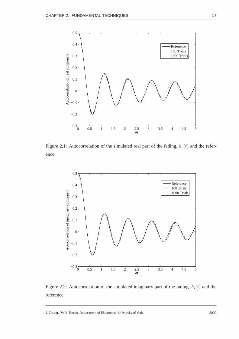
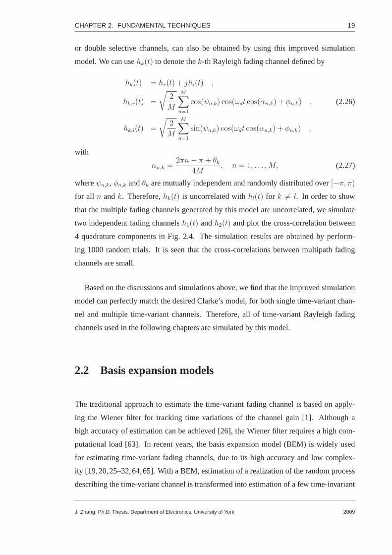
Firstly, we consider the case of a time-variant channel. Fig. 2.1 and Fig. 2.2 show
simulation results for autocorrelations of real and imaginary components of the fading,
respectively, and Fig. 2.3 shows the cross-correlation of the real and imaginary parts of
the fading. The reference is calculated based on (2.7) for the purpose of comparison. Note
thatRhrhi is almost the same asRhihr , therefore, onlyRhihr is shown here.
It is observed that the simulated autocorrelations and cross-correlations match the de-
sired ones closely even whenM is as small as 8 and the number of random trials is only
100. A better match can be obtained if more random trials are performed.
Multiple mutual uncorrelated fading channels, which are required for MIMO channels
J. Zhang, Ph.D. Thesis, Department of Electronics, University of York 2009
CHAPTER 2. FUNDAMENTAL TECHNIQUES 17
0 0.5 1 1.5 2 2.5 3 3.5 4 4.5 5−0.3
−0.2
−0.1
0
0.1
0.2
0.3
0.4
0.5
ντ
Aut
ocor
rela
tion
of r
eal c
ompo
nent
Reference100 Trials1000 Trials
Figure 2.1: Autocorrelation of the simulated real part of the fading,hr(t) and the refer-
ence.
0 0.5 1 1.5 2 2.5 3 3.5 4 4.5 5−0.3
−0.2
−0.1
0
0.1
0.2
0.3
0.4
0.5
ντ
Aut
ocor
rela
tion
of im
agin
ary
com
pone
nt
Reference100 Trials1000 Trials
Figure 2.2: Autocorrelation of the simulated imaginary part of the fading,hi(t) and the
reference.
J. Zhang, Ph.D. Thesis, Department of Electronics, University of York 2009

CHAPTER 2. FUNDAMENTAL TECHNIQUES 18
0 0.5 1 1.5 2 2.5 3 3.5 4 4.5 5−0.2
−0.15
−0.1
−0.05
0
0.05
0.1
0.15
0.2
ντ
Cro
ss−
corr
elat
ion
Reference100 Trials1000 Trials
Figure 2.3: Cross-correlation of the simulated real and imaginary parts of the fading,h(t)
and the reference.
0 0.5 1 1.5 2 2.5 3 3.5 4 4.5 5−0.1
−0.05
0
0.05
0.1
Cro
ss−
corr
elat
ion
0 0.5 1 1.5 2 2.5 3 3.5 4 4.5 5−0.1
−0.05
0
0.05
0.1
ντ
Cro
ss−
corr
elat
ion
Rh
1,ih
2,i
Rh
1,rh
2,r
Reference
Rh
1,rh
2,i
Rh
1,ih
2r
Reference
Figure 2.4: Cross-correlation of two independent fading channelsh1(t) andh2(t) and
reference.
J. Zhang, Ph.D. Thesis, Department of Electronics, University of York 2009
CHAPTER 2. FUNDAMENTAL TECHNIQUES 19
or double selective channels, can also be obtained by using this improved simulation
model. We can usehk(t) to denote thek-th Rayleigh fading channel defined by
hk(t) = hr(t) + jhi(t) ,
hk,r(t) =
√
2
M
M∑
n=1
cos(ψn,k) cos(ωdt cos(αn,k) + φn,k) , (2.26)
hk,i(t) =
√
2
M
M∑
n=1
sin(ψn,k) cos(ωdt cos(αn,k) + φn,k) ,
with
αn,k =2πn− π + θk
4M, n = 1, . . . ,M, (2.27)
whereψn,k, φn,k andθk are mutually independent and randomly distributed over[−π, π)for all n andk. Therefore,hk(t) is uncorrelated withhl(t) for k 6= l. In order to show
that the multiple fading channels generated by this model are uncorrelated, we simulate
two independent fading channelsh1(t) andh2(t) and plot the cross-correlation between
4 quadrature components in Fig. 2.4. The simulation resultsare obtained by perform-
ing 1000 random trials. It is seen that the cross-correlations between multipath fading
channels are small.
Based on the discussions and simulations above, we find that the improved simulation
model can perfectly match the desired Clarke’s model, for both single time-variant chan-
nel and multiple time-variant channels. Therefore, all of time-variant Rayleigh fading
channels used in the following chapters are simulated by this model.
2.2 Basis expansion models
The traditional approach to estimate the time-variant fading channel is based on apply-
ing the Wiener filter for tracking time variations of the channel gain [1]. Although a
high accuracy of estimation can be achieved [26], the Wienerfilter requires a high com-
putational load [63]. In recent years, the basis expansion model (BEM) is widely used
for estimating time-variant fading channels, due to its high accuracy and low complex-
ity [19,20,25–32,64,65]. With a BEM, estimation of a realization of the random process
describing the time-variant channel is transformed into estimation of a few time-invariant
J. Zhang, Ph.D. Thesis, Department of Electronics, University of York 2009

CHAPTER 2. FUNDAMENTAL TECHNIQUES 20
expansion coefficients [64], and the time-variant channel can be modeled as
h = Ba, (2.28)
where theM × 1 vectora = [a1, . . . , aM ]T contains the expansion coefficients, and the
N ×M matrixB = [b1, . . . ,bm, . . . ,bM ] collectsM linearly independent columnsbm.
According to the different ways to generate the matrixB, the family of BEMs can be
categorized into two categories. The first category appliesthe basis functions whose gen-
eration depends on the physical (e.g. fading rate) or statistical information of the fading
channel [20, 29–32, 64], while the second group employs a simple series representation
such as complex exponential or polynomial series [19, 25, 27, 28, 64]. In this section, we
will introduce two BEMs for each category:
The widely used BEMs in the first category are Karhunen-Loeve (KL) [31, 32] and
discrete prolate spheroidal (DPS) [20, 29, 30, 64] BEMs. The generation of KL and DPS
basis functions depends on the knowledge of statistical information of fading. The prob-
lem though is that if the assumed channel statistics deviatefrom the true ones, e.g., due to
inaccurate information of the maximum velocity of the mobile, the performance of these
BEMs may degrade. An alternative approach is to use the secondcategory of BEMs with
fixed functions. In this category, the generalized complex exponential (GCE) and B-spline
(BS) BEMs are widely used.
KL BEM
The KL BEM provides the best performance among these four BEMs [32, 64], since it
assumes that the statistical information of fading is perfectly known at the receiver side.
The KL basis functionsvm(n) are eigenvectors of the fading covariance matrix. For
example, the covariance matrix of Jakes’ fading process is defined as
[Υ]t1,t2 = J0[2πν(t1 − t2)]. (2.29)
We order the eigenvaluesλm of Υ as:λ1 ≥ λ2 ≥ . . . ≥ λN ≥ 0, and assume that when
m is larger than a fixed valueM << N , λm decreases rapidly and can be neglected [32].
Then, the matrixB of the KL BEM can be represented as
[B]n,m = vm(n), m = 1, . . . ,M, n = 1, . . . , N. (2.30)
J. Zhang, Ph.D. Thesis, Department of Electronics, University of York 2009

CHAPTER 2. FUNDAMENTAL TECHNIQUES 21
DPS BEM
Although the modeling error introduced by the KL BEM is insignificant [31, 32], the
covariance matrix of fading is not always available at the receiver side in a practical sce-
nario. Alternatively, a BEM based on DPS functions was proposed in [20]. The DPS
BEM corresponds to the discrete KL BEM with a rectangular spectrum [20]. The DPS
basis functions are also named Slepian sequences, which arebandlimited to the Doppler
spread[−ν, ν] and simultaneously most concentrated in the certain time interval of length
M [66]. DPS sequences are widely used for channel estimation both in time and fre-
quency domains [20, 30, 67]. Here we will introduce the principle of DPS sequences
briefly.
The target is to find the sequencesu[m] which maximize the energy concentration in
the interval with lengthN [20]
λ =
∑N−1n=0 |u[n]|2
∑∞n=−∞|u[n]|2
, (2.31)
while being bandlimited toν; hence
u[n] =
∫ ν
−ν
U(ν)ej2πnνdν, (2.32)
where
U(ν) =∞∑
n=−∞
u[n]e−j2πnν , (2.33)
and0 ≤ λ ≤ 1.
The solution of this constrained maximization problem are the DPS sequences [66],
which are the eigenvectors of the following eigenvalue equation
N∑
q=1
sin(2πν(q − n))
π(q − n)um(q) = λmum(n), (2.34)
whereum(n) is themth basis function with lengthN bandlimited to the frequency range
[−ν, ν], andλm is an eigenvalue indicating the fraction of energy contained in the fre-
quency range[−ν, ν] of the corresponding eigenvector [67].
The DPS sequenceu0[n] is the unique sequence that is bandlimited and most time-
concentrated in a given interval with lengthN , u1[n] is the next sequence having maxi-
mum energy energy concentration among the DPS sequences orthogonal tou0[n], and so
J. Zhang, Ph.D. Thesis, Department of Electronics, University of York 2009

CHAPTER 2. FUNDAMENTAL TECHNIQUES 22
on. Thus, the DPS sequences are a set of orthogonal sequenceswhich are bandlimited
and high (but not complete) time-concentrated in a certain interval with lengthN [20].
The eigenvaluesλm are a measure for this energy-concentration and ordered starting with
the maximum one asλ1 ≥ λ2 ≥ . . . ≥ λN ≥ 0. Therefore,um(n) is themth function
corresponding to themth most maximum eigenvalue;M should be chosen to provideλm
close to 1 whenm << M and close to 0 whenm >> M [29]. The option ofM is
described in [66], as
M = 2⌈νN⌉+ 1, (2.35)
⌈x⌉ denotes the smallest integer value larger than or equal tox. The rigorous proof can
be found in [68]. Then, the matrixB containing samples of the DPS basis functions can
be represented as
[B]n,m = um(n), m = 1, . . . ,M, n = 1, . . . , N. (2.36)
GCE BEM
The GCE BEM, which is also known as oversampled complex exponential (CE)
model [25] or non-critically sampled CE model [69], is a modified model of the the CE
BEM. The CE BEM is introduced in [19] to approximate the time variant fading channels.
Its basis functions are complex exponentials that have a period equal to the length of the
considered interval. Normally, the channel modeled by CE BEM is represented as [23,70]
h(n) =M∑
m=1
amej2π
N(n−1)[(m−1)−M/2], m = 1, . . . ,M, n = 1, . . . , N. (2.37)
Although the CE BEM is widely used to approximate the time-variant fading channel [21,
23, 71–74], the modeling error of CE BEM is significant. The rectangular window in
(2.37), which corresponds to critically sampling the Doppler spectrum, results in spectral
leakage, which means, the energy from low frequency CE coefficients leaks to the full
frequency range [20]. This results in a floor in the BER performance for time-variant
channels with Doppler spread as shown in [75].
Since only a limit Doppler range of windowed channel is considered, the sidelobes
might be significantly eliminated and more samples are takenin within that range [25].
An improved modeling performance is obtained by using the GCEBEM, which applies a
J. Zhang, Ph.D. Thesis, Department of Electronics, University of York 2009

CHAPTER 2. FUNDAMENTAL TECHNIQUES 23
set of complex exponentials with the period longer than the window length related to the
CE BEM [25,70]. This corresponds to oversampling the Doppler spectrum of windowed
channel. For the GCE BEM, elements of the matrixB are given by [25,70]
[B]n,m = ej2π
κN(n−1)[(m−1)−M/2], m = 1, . . . ,M, n = 1, . . . , N, (2.38)
whereκ is a real number larger than1; usually,κ = 2 is used [25].
BS BEM
The B-splines have previously been investigated in application to estimating the Clarke’s
model [26–28,65,76] since its high approximation accuracyand low computational com-
plexity. An optimal spline of orderq, approximating the random processh(t) with zero
mean and varianceσ2h, is a spline providing an MSE which is defined as
ε2 =1
σ2hT
∫ T
0
E[h(t)− h(t)]2dt, (2.39)
whereh(t) is an approximation ofh(t) by applying splines, andT is the sampling interval.
An optimal spline of orderq can be represented as
h(t) =m=∞∑
−∞
ambq(t−mT ), (2.40)
wherebq(t) is the B-spline of orderq, andam are spline coefficients.bq(t) is a (q + 1)
fold convolution of the B-spline of zero degree [77]
b0(t) =
1, if |t| < T2
12, if |t| = T
2
0, otherwise,
(2.41)
whereT is the sampling interval. Usually,bq(t) are described by the Fourier trans-
form [27]
Bq(ω) =
∫ ∞
−∞
bq(t)e−jωtdt = T
[
sin(ωT2)
ωT2
]q+1
. (2.42)
The optimal spline approximation can be described by a “prefilter-sampling-postfilter”
scheme which is shown in Fig.2.5 [27] whereG(ω) andF (ω) are transfer functions of
the prefilter and postfilter, andδ(t) is the Dirac delta function [78]. The postfilter transfer
J. Zhang, Ph.D. Thesis, Department of Electronics, University of York 2009

CHAPTER 2. FUNDAMENTAL TECHNIQUES 24
Figure 2.5: Prefilter-sampling-postfilter scheme describing spline approximation of the
processx(t),
functionF (ω) is the Fourier transform of the B-splines,F (ω) = Bq(ω), while the prefilter
has the transform function [27]
G(ω) =
[
(ωT
2) sin(
ωT
2)
]−q−1
×[
∞∑
n=−∞
(
ωT
2+ nπ
)−2q−2]−1
. (2.43)
If the the random processh(t) obeys Clarke’s model, the MSE of the approximation by
applying optimal splines of an arbitrary orderq can be calculated by [27]
ε2 ≈ π2q+2B2q+2
[(q + 1)!]2γ2q+2+π2q+4(q + 1)(2q + 3)B2q+4
[(q + 2)!]2γ2q+4, (2.44)
whereBn are Bernoulli numbers [79], and the sampling factorγ = 1/(νT ).
To build the basis functions, we use the B-spline of orderq [76]
Bq(t) =1
q!
q+1∑
i=0
(−1)i(
q + 1
i
)(
t
T+q + 1
2− i
)q
+
, (2.45)
whereT = (N−1)/(M−q) is the sampling interval separating two adjacent BS functions,
and(x)+ = max0, x. In this case, elements of the basis function matrix are given by
[B]n,m = Bq
(
(n− 1)−(
m− q + 1
2
)
T
)
, m = 1, . . . ,M, n = 1, . . . , N.
(2.46)
The accuracy and complexity of B-spline approximation depend on the orderq of the
spline.
As shown above, the KL and DPS BEMs can approximate the time-variant fading
channel with insignificant modeling error but require the statistics of fading and have to
J. Zhang, Ph.D. Thesis, Department of Electronics, University of York 2009

CHAPTER 2. FUNDAMENTAL TECHNIQUES 25
suffer extra error caused by inaccurate estimation of thesestatistics. Although the GCE
and BS BEMs do not require the knowledge of the statistical information of fading by
using a simple series representation as basis functions, they will introduce higher model-
ing errors than KL and DPS BEMs. We will compare the performance and complexity of
these four BEMs in Chapter 3 and use the one which can provide a good performance and
affordable complexity to approximate the fading channels in this thesis.
2.3 Turbo codes
Turbo codes were first introduced by Berrou, Glavieux and Thitimajshima at the Inter-
national Conference on Communication (ICC) in 1993 [80]. In AWGN channels, the
performance of a half rate turbo code is only 0.7 dB away from the Shannon capacity
limit at BER= 10−5. The remarkable achievement terminates the conventional thought
that the Shannon limit can only be approached by using extraordinarily long codes with
extremely complex decoding processes [81]. As one of the most powerful error-control
codes, Turbo codes have been developed rapidly and attract substantial attention in wire-
less communication community due to its outstanding ability of error correction [82–88].
Turbo codes are based on two fundamental concepts, concatenated coding and iterative
decoding, the latter of which is the core of the ‘turbo principle’ since it is the method
that allows the outstanding performance of turbo codes. As turbo codes will be used in
some chapters of this thesis, we will briefly introduce the structure of the turbo encoder
and main turbo decoding algorithms, i.e., the optimal maximum a posteriori(MAP) and
Log-MAP algorithms, and the suboptimal MAX-Log-MAP algorithm. For more detailed
description of turbo codes, readers are referred to [89–91].
2.3.1 Turbo encoder
The structure of the turbo encoder used in this report can be explained by its formal name,
parallel concatenated recursive systematic convolutional (RSC) code. Fig. 2.6 gives an
example of the structure of a turbo encoder. Two RSC encoders are concatenated and
J. Zhang, Ph.D. Thesis, Department of Electronics, University of York 2009

CHAPTER 2. FUNDAMENTAL TECHNIQUES 26
an interleaver is in between them. Comparing with non-systematic convolutional (NSC)
codes, RSC codes apply a feedback loop (recursive part) and set one of the outputs equal
to the input data (systematic part). The structure of a RSC encoder and the corresponding
NSC encoder are shown in Fig. 2.7 and Fig. 2.8, respectively.For both encoders, the
code rate is1 and the constraint length is3. The generator polynomials of the feedback
and output connectivity in the RSC encoder are[7, 5] in octal notations, respectively.
The working principles of the turbo encoder are described here. A lengthN data
sequenced = [d[1], . . . , d[N ]] is encoded by the first RSC encoder, the output of which
is a lengthN coded sequencex1p = [x1p[1], . . . , x
1p[N ]]. Then, the original data sequence
is interleaved and encoded by the seconde RSC encoder to generate another lengthN
coded sequencex2p = [x2p[1], . . . , x
2p[N ]]. Finally, d, x1
p andx2p are multiplexed together
to generate the final turbo coded sequence. Without puncturing, this results in a code rate
of 1/3. Higher code rates can be obtained by applying a puncturing scheme.
Figure 2.6: Structure of a Turbo encoder.
The interleaver is a device that simply reorders the input data sequence, while an dein-
terleaver, which will be used in the decoder to recover the original order of the data se-
quence. It is the joint influence of the interleaver and RSC encoder leading to a high code
weight composite codeword for most of the time which is critical to the performance of
turbo code [92]. There are numerous interleavers that can beused in the turbo encoders,
i.e. pseudo-random [93], block [94], and s-random interleavers [95–98]. In this report, we
apply the s-random interleaver due to its superior performance [90]. The output pattern
J. Zhang, Ph.D. Thesis, Department of Electronics, University of York 2009

CHAPTER 2. FUNDAMENTAL TECHNIQUES 27
Figure 2.7: Example of a Recursive Systematic Convolutional (RSC) encoder.
of such an interleaver is generated randomly, with the constraint that any two input bits at
a distance smaller thans bits will be separated by at leasts bits after interleaving.
2.3.2 Turbo decoder
Fig. 2.9 illustrates the turbo decoder corresponding to theencoder in Fig. 2.6. It is seen
that two RSC decoders are linked by an deinterleaver/interleaver, which is similar to that
used in the encoder.
The turbo decoder works iteratively and in each iteration the two RSC decoders ex-
change the decoded information to help each other. Before decoding iterations, the re-
ceived signalsy[k] = (yd[k], y1p[k], y
2p[k]) from the demodulator are demultiplexed to
sequencesyd[k], y1p[k] andy2p[k], respectively, whereyd[k] corresponds to the received
systematic codes,y1p[k] corresponds to the received 1st parity bits, andy2p[k] corresponds
to the received 2nd parity bits. The first RSC decoder appliesyd[k] andy1p[k] as input
sequences and the second RSC decoder appliesyd[k] andy2p[k]. When the parity bits of a
given RSC encoder are punctured before transmission, the corresponding decoder’s inputs
are set to zeros at the punctured positions. In the initial iteration, the first RSC decoder
takes onlyyd[k] andy1p[k] to generate soft information of the data bits,LE,1(d[k]). Then
the second RSC decoder can perform decoding with the soft information ofLE,1(d[k])
J. Zhang, Ph.D. Thesis, Department of Electronics, University of York 2009

CHAPTER 2. FUNDAMENTAL TECHNIQUES 28
Figure 2.8: Example of a Non-Systematic Convolutional (NSC) encoder.
andLap,1(d[k]) from the first RSC decoder, in addition to the receivedyd[k] andy2p[k].
The output of the second decoder is another soft decoding informationLE,2(d[k]), which
will be deinterleaved to generateLap,2(d[k]) and fed back to the first RSC decoder. In
the subsequent iterations, the first RSC decoder takesLap,2(d[k]) from the second RSC
decoder in the previous iteration as additional information to yd[k] andy1p[k], to generate
LE,1(d[k]). The performance of the turbo decoder improves as the numberof iterations
increases. However, the improvement from iteration to iteration decreases as the num-
ber of iterations increases. This process is repeated iteratively until two RSC decoders’s
estimates of the original data bits converge. Eight iterations are commonly used, as a
compromise between the performance and complexity [81]. Finally, the outputa pos-
teriori informationL(d[k]) of a data bitd[k] delivered from the second RSC decoder is
deinterleaved and used for the final hard decision.
In general, each RSC decoder performs decoding by using its input received signals
(yd[k] andyip[k], i = 1, 2) and thea priori information (Lap,i(d[k]), i = 1, 2) from the other
RSC decoder, and provides the extrinsic informationLE,i(d[k]) for the other decoder.
Note that the extrinsic information is only exchanged between decoders as intermediate
information during the decoding process. The soft information exchanging between two
RSC decoders is the reason why the turbo decoder is called soft-input soft-output decoder,
J. Zhang, Ph.D. Thesis, Department of Electronics, University of York 2009

CHAPTER 2. FUNDAMENTAL TECHNIQUES 29
Figure 2.9: Structure of a Turbo decoder.
which accepts softa priori informationLap,i(d[k]) at one of its inputs from the previous
decoding process and generates soft informationLE,i(d[k]) as its output. Soft information
means that besides decoded bits, the associated probability that each bit has been decoded
correctly is also provided, usually in the form of log-likelihood ratio (LLR). This indicates
that the decoder yields not only the coded bits but also how reliable they are. As its name
implies, the LLR is the logarithm of the ratio of two probabilities in the case of binary
transmission, e.g., the outputa posterioriinformation (L(d[k])) is generally given by
L(d[k]) = logP (d[k] = +1|y)P (d[k] = −1|y) , (2.47)
where the numerator and denominator are probabilities of the transmitted bitd[k] = +1
andd[k] = −1 conditioned on the received sequencey. Based on (2.47), the more positive
the value ofL(d[k]) is, the more reliably the transmitted bit was ‘1’, or the morenegative
the value ofL(d[k]) is, the more likely ‘0’ was transmitted.
In the turbo decoder shown in Fig. 2.9, the outputL(d[k]), a posterioriinformation of
an information bitd[k], is a sum of
L(d[k]) = L(d[k]) + Lap(d[k]) + LE(d[k]) , (2.48)
J. Zhang, Ph.D. Thesis, Department of Electronics, University of York 2009

CHAPTER 2. FUNDAMENTAL TECHNIQUES 30
whereL(d[k]) is the channel information,Lap(d[k]) is the a priori information and
LE(d[k]) is the extrinsic information.
The channel informationL(d[k]) can be extracted directly fromy[k] which are the
received signals ofd[k]. Supposing thatd[k] are transmitted withEs transmitted energy
per symbol, over an AWGN channel, the received signal is
y[k] = a · d[k] + n[k] , (2.49)
wherenk denotes an AWGN with a variance ofσ2n, anda is the fading amplitude in a
fading channel or a constant value in an AWGN channel. For sucha model, the channel
information is given by [81]
L(d[k]) = logexp
(
− Es
2σ2n(y[k]− a)2
)
exp(
− Es
2σ2n(y[k] + a)2
)
= log
(
exp
(
2aEsσ2n
y[k]
))
= Lc · y[k], (2.50)
whereLc = 2aEs/σ2n is the channel reliability factor, which reflects the reliability of
estimating the transmitted signal from the received signal. For example,Lc will be large
if SNR in the channel is high, and we can estimate the transmitted signal from the received
signal correctly with a high probability. In such a case, thereceived signal will impact
heavily on the final outputa posterioriLLR.
Thea priori informationLap(d[k]) used here is the deinterleaved extrinsic information
from the other RSC decoder.
The extrinsic informationLE(d[k]) is the information that decoder exploits from the
whole received sequence anda priori information, but excludes these of the bits which
are currently being decoded in this iteration. It is only theextrinsic information that the
decoders exchange between each other since the same information should not be used
more than once at each decoding step.
Taking all these three types of information above into account, the turbo decoder de-
livers thea posterioriinformation of data bits. The final decision of the decoding is based
on thea posterioriinformation of data bits.
J. Zhang, Ph.D. Thesis, Department of Electronics, University of York 2009

CHAPTER 2. FUNDAMENTAL TECHNIQUES 31
There are 3 typical decoding algorithms applied widely: MAPalgorithm, MAX-Log-
MAP algorithm and Log-MAP algorithm [80,92,99–102]. All ofthese algorithm will be
introduced briefly in follows.
The Maximuma Posteriorialgorithm was firstly proposed by Bahl, Cocke, Jelinek
and Raviv in [92] and modified by Berrou, Glavieuv and Thitmajshima in [80]. Com-
pared with the conventional maximum likelihood sequence estimation (MLSE) algorithm
which can be efficiently implemented by the Viterbi algorithm [103], the MAP algorithm
is a symbol-by-symbol detection algorithm based on maximuma posterioriinformation.
It is optimal in the sense of minimizing the probability of a symbol error by takinga
priori information of the coded bits into account and providing soft information about
estimated bits. The performance of the MAP and MLSE algorithms would be the same
when there is noa priori information to be exploited. However, whena priori informa-
tion is available, for example, in the soft-input soft-output turbo decoder exchanging the
extrinsic information between two RSC decoders, the MAP algorithm will outperform the
conventional MLSE one [80].
Although the MAP algorithm is the optimal decoding scheme, it is too complicated
to be realized for implementation since the exact representation of probabilities used in
the MAP algorithm requires a high dynamic range [81]. Moreover, there are many non-
linear functions and numerous multiplications proposed inthe scheme [81]. Working in
the logarithmic domain instead of the linear domain for the probability used in the MAP
algorithm and invoking the approximation
ln(ex1 + . . .+ exn) ≈ maxi∈1,2...,n
xi, (2.51)
the MAX-Log-MAP algorithm reduces the complexity significantly. However, it is obvi-
ous that the MAX-Log-MAP algorithm is suboptimal since onlya part of information is
exploited due to the approximation.
This approximation can be avoided by applying the Jacobian logarithm to calculate
x = ln(ex1 + . . .+ exn). The Jacobian logarithm [104,105] is given by
ln(ex1 + ex2) = max(x1, x2) + ln(1 + e−|x1−x2|)
= max(x1, x2) + fc(|x1 − x2|)
= gc(x1, x2), (2.52)
J. Zhang, Ph.D. Thesis, Department of Electronics, University of York 2009

CHAPTER 2. FUNDAMENTAL TECHNIQUES 32
wherefc(|x1 − x2|) can be regarded as a correction term. Robertson, Hoeher and Ville-
brun in [100] proposed a method to show how to use the Jacobianlogarithm to calculate
ln(ex1 + . . .+ exn) accurately. They supposedx = ln(ex1 + . . .+ exn−1) is known. Then,
they obtained
ln(ex1 + . . .+ exn) = ln(ex + exn)
= max(x, xn) + fc(|x− xn|). (2.53)
This method is referred to as the Log-MAP algorithm [100]. Itwas also shown that the
correction termfc(|x1−x2|) can be implemented efficiently by an one dimension look-up
table to avoid real time computation, moreover, only a few values are needed for the table.
By applying the Jacobian logarithm, the Log-MAP algorithm retains the optimality of the
original MAP algorithm, while preserves the computationalsimplicity of the MAX-Log-
MAP algorithm. For interested readers, more details about the MAP, MAX-Log-MAP
and Log-MAP algorithms can be obtained from [99,101,102].
0 0.2 0.4 0.6 0.8 1 1.2 1.410
−7
10−6
10−5
10−4
10−3
10−2
10−1
100
Eb/N
0, dB
BE
R
1st iteration2nd iteration3th iteration4th iteration5th iteration8th iteration10th iteration
Figure 2.10: BER performance of turbo codes with rate 1/3, 8 states, 1024 bits, Log-MAP,
over AWGN channels.
Fig. 2.10 shows the BER performance of the turbo codes over theAWGN channels.
A turbo code with rate1/3, 8 states is employed in the simulation. The generator polyno-
mials of the RSC encoders are[13, 15] in octal for their feedback and output connections
respectively. The length of frame is 1024, giving a sufficient s-parameter of 20 for the
s-random interleaver. The turbo decoder applies the Log-MAPalgorithm and the number
J. Zhang, Ph.D. Thesis, Department of Electronics, University of York 2009

CHAPTER 2. FUNDAMENTAL TECHNIQUES 33
of decoding iterations are 1, 2, 3, 4, 5, 8 and 10. Simulation results show that the BER
performance of turbo codes improves but the improvement between two consecutive it-
erations decreases as the number of iterations increases. When the number of iterations
is larger than8, the improvement almost decreases to zero. Thus, in this thesis, we will
apply 8 turbo decoding iterations in simulations.
2.4 Conclusions
In this chapter, we have introduced fundamental techniques, such as the simulator of time-
variant channels, BEMs and Turbo codes, which will be used throughout this thesis. After
briefly introducing the reference Clarke’s model and the deficiencies of Jakes’ model and
Pop-Beaulieu simulator, we have adopted the model introduced by Zheng and Xiao [51,
57] to generate multiple fading channels. We have also provided simulation results for
second-order statistics of this model, which have shown that this model can accurately
match to the desired Clarke’s model. Therefore, all time-variant channels considered in
this thesis are generated by using this improved simulationmodel.
We have also introduced BEMs used to approximate the fading channels. Advantages
and disadvantages of the most widely used BMEs, such as KL, DPS, GCE and BS BEMs,
have been briefly discussed. In the next chapter, we will compare these four BEMs in
application to time-variant fading channels and will show that the BS BEM is the best
practical choice providing good performance and low complexity.
Finally, we have introduced the turbo encoder and decoder with different decoding al-
gorithms, such as MAP algorithm, MAX-Log-MAP algorithm andLog-MAP algorithm.
After describing the advantages and disadvantages of each decoding algorithm, we have
chosen Log-MAP decoding algorithm and will be using it in thesubsequent chapters to
realize the soft-input soft-output turbo decoding schemes.
J. Zhang, Ph.D. Thesis, Department of Electronics, University of York 2009

Chapter 3
Channel Estimation of Time-Varying
Channels Based on Basis Expansion
Models
Contents
3.1 Introduction . . . . . . . . . . . . . . . . . . . . . . . . . . . . . . . 34
3.2 Transmission model and BEMs . . . . . . . . . . . . . . . . . . . . . 36
3.3 MSE of a generic linear channel estimator . . . . . . . . . . . . . . 40
3.4 Approach 1: Channel estimation using perfect knowledge of the
Doppler spread . . . . . . . . . . . . . . . . . . . . . . . . . . . . . . 43
3.5 Approach 2: Channel estimation using the maximum Doppler spread 49
3.6 Approach 3: Channel estimation using an estimate of the Doppler
spread . . . . . . . . . . . . . . . . . . . . . . . . . . . . . . . . . . 53
3.7 Conclusions . . . . . . . . . . . . . . . . . . . . . . . . . . . . . . . 59
3.1 Introduction
In mobile communications, the Doppler effect causes the time variant fading. The pa-
rameter used to measure this Doppler effect is the Doppler spread. Usually, this fading is
J. Zhang, Ph.D. Thesis, Department of Electronics, University of York
34
2009

CHAPTER 3. CHANNEL ESTIMATION OF TIME-VARYING CHANNELS BASED ON BASIS
EXPANSION MODELS 35
well described by Jakes’ model [50], or more generally, by Clarke’s model [49,106]. For
Jakes’ model, the channel gain is a stationary random process with a correlation function
described as the zero-order Bessel function of the first kind parameterized by the Doppler
spread.
In order to approximate the time-variant fading channels, basis expansion mod-
els (BEMs) are widely used [19, 20, 25–32, 64, 65]. The most often used BEMs are
the Karhunen-Loeve (KL) functions [31, 32], discrete prolate spheroidal (DPS) func-
tions [20, 29, 30, 64], generalized complex exponential (GCE) functions [19, 25, 64], and
B-splines (BS) [26–28,65]. With a BEM, estimation of a realization of the random process
describing the time-variant channel is transformed into estimation of a few time-invariant
expansion coefficients [20].
The MSE performance of BEM-based channel estimators is considered in [20, 32, 64,
69, 107–109]. Analytical results in [32, 107, 108] are basedon the assumption that the
Doppler spread is perfectly known, whereas in practice, theDoppler spread is estimated
with some errors [110]. In [20], instead of assuming that theDoppler spread is perfectly
known, the maximum Doppler spread is used to generate the DPSbasis functions. This
method is widely used in the works investigating the DPS BEM [64, 109]. Although the
use of the maximum Doppler spread is more practical and may reduce the complexity of
BEM-based estimators, it may also lead to a significant degradation in the MSE perfor-
mance.
The Doppler spread can be estimated based on correlation andvariation of channel
estimates. For example, in [111], the Doppler estimation scheme based on the autocor-
relation of complex channel estimates is described. Instead of using channel estimates,
the received signal can also be used directly in estimating Doppler spread information.
In [112], the mobile speed is estimated as a function of the deviation of the averaged sig-
nal envelope in flat fading channels. In [110], an efficient Doppler estimation algorithms
for wireless mobile radio systems is introduced by using an ML approach relying on a
periodic channel estimation. In [69], the performance of BEM-based MMSE estimators
using the mismatched Doppler spread has been investigated.However, the derivation of
MSE in [69] is limited to the MMSE estimator using BEMs with orthogonal basis func-
tions; as a result, it cannot be applied to the BS and GCE BEMs.
J. Zhang, Ph.D. Thesis, Department of Electronics, University of York 2009

CHAPTER 3. CHANNEL ESTIMATION OF TIME-VARYING CHANNELS BASED ON BASIS
EXPANSION MODELS 36
In this chapter, we derive the MSE of a generic linear channelestimator using lin-
early independent basis functions, and specify the error for MMSE and ML estimators.
The MSE performance of the Wiener solution is considered andused as a lower MSE
bound. We then investigate and compare the MSE performance and complexity for three
approaches to estimating time-variant channels with perfect or inaccurate knowledge of
the Doppler spread:
1) channel estimation using perfect knowledge of the Doppler spread;
2) channel estimation using the maximum Doppler spread as suggested in [20];
3) channel estimation using an estimate of the Doppler spread.
The first approach provides the best MSE performance; however, it might be very com-
plicated depending on the BEM used and the assumption of a perfectly known Doppler
spread is impractical. Both the second and third approaches are based on inaccurate
knowledge of the Doppler spread; we will investigate which one can provide a better
MSE performance and lower complexity. The complexity of each approach depends on
the BEM used. Therefore, we will compare the MSE performance and complexity of
estimators using different BEMs for each approach, and give apractical choice of the
approach and BEM providing the best performance and the lowest complexity.
The remainder of this chapter is organized as follows. In Section 3.2, the transmission
model and different BEMs are introduced. Section 3.3 describes the MSE derivation for
a generic BEM-based linear channel estimator. The performance and complexity of the
first approach using perfect knowledge of the Doppler spreadare described in Section 3.4.
Then, the MSE performance and complexity of the second and third approaches both
based on inaccurate knowledge of the Doppler spread are investigated and compared in
Section 3.5 and Section 3.6, respectively, followed by conclusions in Section 3.7.
3.2 Transmission model and BEMs
We consider a PSAM system and assume that a block ofN pilot symbols is transmitted
and there areNd data symbols transmitted between two neighboring pilot symbols, e.g.
as shown in Fig. 3.1. The received pilot signal can be writtenin the time-domain as
z(i) = s(i)h(i) + n(i), i = 0, · · · , N − 1, (3.1)
J. Zhang, Ph.D. Thesis, Department of Electronics, University of York 2009

CHAPTER 3. CHANNEL ESTIMATION OF TIME-VARYING CHANNELS BASED ON BASIS
EXPANSION MODELS 37
Figure 3.1: Structure of transmitted block.
where at theith observed instance,s(i) is the transmitted pilot symbol of a power|s(i)|2 =σ2s , h(i) is the (time variant) channel coefficient andn(i) is the complex additive white
Gaussian noise (AWGN) with zero mean and varianceσ2n. The matrix form of (3.1) is
given by
z = Sh+ n, (3.2)
wherez, h andn areN × 1 vectors with elementsz(i), h(i) andn(i), respectively, andS
is anN ×N diagonal matrix with diagonal elementss(i).
We consider time-variant Rayleigh fading channels following Jakes’ model [50, 51].
The covariance matrix of such a channel is anN ×N matrixΥ with elements
[Υ]t1,t2 = ρ(t1 − t2), (3.3)
wheret1, t2 = 1, . . . , N , andρ(τ) is the autocorrelation function [50]
ρ(τ) = σ2hJ0(2πντ), (3.4)
σ2h is the variance of channel coefficients,J0(·) is the zero-order Bessel function of the
first kind andν is the Doppler spread.
The time-variant fading channel can be represented by a BEM. We define anN ×M
matrixB containing samples of basis functions corresponding toN transmitted symbols,
whereM is the number of basis functions. The time-variant channel can be modeled as
h = Ba, (3.5)
where the vectora = [a1, . . . , aM ]T contains the expansion coefficients and[·]T denotes
matrix transpose. The difference betweenh andh is due to a modeling error. By applying
J. Zhang, Ph.D. Thesis, Department of Electronics, University of York 2009

CHAPTER 3. CHANNEL ESTIMATION OF TIME-VARYING CHANNELS BASED ON BASIS
EXPANSION MODELS 38
a BEM, the task of estimatingN time varying channel coefficients is transformed into
estimating onlyM expansion coefficients with usuallyM << N . As mentioned above,
we will consider the following BEMs: KL, DPS, GCE, and BS basis functions.
KL BEM
The KL BEM is introduced in [32,107] as a BEM with perfect knowledge of the statistical
information of fading channels. The KL basis functionsvm(n) are the eigenvectors of the
covariance matrix of the fadingΥ, which is obtained in (3.3). We order the eigenvalues
λm of Υ asλ1 ≥ λ2 ≥ . . . ≥ λN ≥ 0. Then, the matrixB of the KL BEM can be
represented as
[B]n,m = vm(n), m = 1, . . . ,M, n = 1, . . . , N. (3.6)
DPS BEM
The DPS functions are a set of orthogonal functions bandlimited to the range[−ν, ν].We considerM basis functionsum(n) of lengthN . Such sequences are defined as the
real-value solution of the following equation [20]
N−1∑
q=0
sin(2πν(q − n))
π(q − n)um(q) = λmum(n), n = 0, . . . , N − 1, (3.7)
whereλm andum are the eigenvalues and eigenvectors of the matrix
[C]i,j =sin(2πν(i− j))
π(i− j), i, j ∈ 1, . . . , N. (3.8)
λm indicates the fraction of energy ofum(n) contained in the range[−ν, ν] [67]. The
eigenvalues are ordered in the descending orderλ1 ≥ λ2 ≥ . . . ≥ λN ≥ 0. Then, the
matrixB of the DPS BEM can be represented as
[B]n,m = um(n), m = 1, . . . ,M, n = 1, . . . , N. (3.9)
J. Zhang, Ph.D. Thesis, Department of Electronics, University of York 2009

CHAPTER 3. CHANNEL ESTIMATION OF TIME-VARYING CHANNELS BASED ON BASIS
EXPANSION MODELS 39
GCE BEM
For the GCE BEM, elements of the matrixB are given by [25,70]
[B]n,m = ej2π
κN(n−1)((m−1)−(M−1)/2), m = 1, . . . ,M, n = 1, . . . , N, (3.10)
whereκ is a real number larger than1. Forκ = 1, the GCE BEM becomes the complex
exponential (CE) BEM. However, the CE BEM results in a large modeling error [25,70].
The GCE BEM introduces a lower modeling error; usually,κ = 2 is used [25].
BS BEM
The B-splines have previously been investigated in application to estimating the Clarke’s
model [26–28,65]. To build the basis functions, we use the B-spline of orderq [76]
Bq(t) =1
q!
q+1∑
i=0
(−1)i(
q + 1
i
)(
t
T+q + 1
2− i
)q
+
, (3.11)
whereT = (N − 1)/(M − q) is the sampling interval separating two adjacent B-spline
functions, and(x)+ = max0, x. In this case, elements of the basis function matrix are
given by
[B]n,m = Bq
(
(n− 1)−(
m− q + 1
2
)
T
)
, m = 1, . . . ,M, n = 1, . . . , N.
(3.12)
The accuracy and complexity of B-spline approximation depend onq, and normally, the
B-spline of orderq = 3 is widely used since it provides the trade-off between complexity
and accuracy [27,76]. Here, we use the cubic BS BEM and compare its performance and
complexity with those of the other BEMs. For this case, from (3.11) we have
B3(t) =
23− t2
T 2 +|t|3
2T 3 , if |t| < T,
16(2− |t|
T)3, if T ≤ |t| < 2T ,
0, otherwise,
(3.13)
and (3.12) becomes
[B]n,m = B3 ((n− 1)− (m− 2)T ) , m = 1, . . . ,M, n = 1, . . . , N. (3.14)
J. Zhang, Ph.D. Thesis, Department of Electronics, University of York 2009

CHAPTER 3. CHANNEL ESTIMATION OF TIME-VARYING CHANNELS BASED ON BASIS
EXPANSION MODELS 40
It is clear that for cubic B-splines, theN ×M matrixB is a sparse matrix, and there are
only 4 nonzero elements in each row andK nonzero elements in each column, where
K = ⌈4T ⌉ = ⌈4(N − 1)/(M − 3)⌉, (3.15)
and⌈x⌉ denotes the smallest integer value larger than or equal tox.
3.3 MSE of a generic linear channel estimator
3.3.1 BEM-based estimator
A BEM-based channel estimate is given by
h = Ba, (3.16)
wherea is a vector of estimates of expansion coefficients, the estimation ofh is transfer-
ring to the estimation ofa. In this chapter, we consider linear channel estimators based
on BEMs, i.e., ML channel estimator and MMSE channel estimator.
The ML channel estimator has the asymptotic properties of being unbiased and have
a Gaussian PDF [113]. We consider the case with white Gaussian noise with PDF
NC(0, σ2nIN). Under these condition the PDF of received signalz is [113]
p(z; a) =1
(2π)N/2 σnNexp
[
−1
2(z− SBa)H (z− SBa)
]
, (3.17)
therefore, the ML channel estimation ofa is found by minimizing
J(a) = (z− SBa)H (z− SBa) . (3.18)
Since this is a quadratic function of the elements ofa andσ2nIN is a positive definite
matrix, differentiation will produce the global minimum [113]. Thus, we have
∂ ln p(z; a)
∂a=∂J(a)
∂a= σ−2
n
∂(SBa)H
∂a(z− SBa). (3.19)
By setting (3.19) equal zero we have
SBH(z− SBa) = 0. (3.20)
J. Zhang, Ph.D. Thesis, Department of Electronics, University of York 2009

CHAPTER 3. CHANNEL ESTIMATION OF TIME-VARYING CHANNELS BASED ON BASIS
EXPANSION MODELS 41
Therefore, the ML estimate ofa is given by [113]
aML = (BHSHSB)−1BHSHz. (3.21)
The MMSE channel estimator solving the estimation problem by minimizing
J(a) = E
(z− SBa)H (z− SBa)
. (3.22)
In (3.22), since the matricesS andB and vectorz are perfectly known, the only random
unknown variable is the vectora. Therefore, the expectation in (3.22) is overa. We can
solve the estimation problem by set
∂J(a)
∂a= 0. (3.23)
After some algebra, we obtain the MMSE estimates ofa as [113]
aMMSE = Ea+(
BHSHSB+ σ2n
(
EaaH)−1)−1
BHSH(z− SBEa). (3.24)
Here we consider the Rayleigh fading channels and therefore,we haveEa = 0 and
we define thatEaaH = Ra is the covariance matrix of expansion coefficients, and
represented as [65]
Ra = (BHB)−1BHΥB(BHB)
−1. (3.25)
Then, (3.24) is simplified as [113]
aMMSE =(
BHSHSB+ σ2nR
−1a
)−1BHSHz. (3.26)
Considering a general expression of a BEM-based linear channel estimator, the vector
a can be represented as
a = Az, (3.27)
whereA is a matrix defined by the channel estimation scheme. For MMSEestimation,
we have
AMMSE = (BHSHSB+ σ2nR
−1a )−1BHSH . (3.28)
For ML channel estimation, we have
AML = (BHSHSB)−1BHSH . (3.29)
J. Zhang, Ph.D. Thesis, Department of Electronics, University of York 2009

CHAPTER 3. CHANNEL ESTIMATION OF TIME-VARYING CHANNELS BASED ON BASIS
EXPANSION MODELS 42
Here we derive the MSE of a generic BEM-based linear estimatorand specify it for
different estimation schemes. The MSE is represented as
MSE=1
tr E [hhH ] tr
E
[
(
h− h)(
h− h)H]
, (3.30)
where tr· denotes the trace operator,(·)H denotes the Hermitian transpose andE[·]denotes the expectation. By substituting (3.16) and (3.27) into (3.30), we obtain
MSE=1
tr Υ tr
E[
(h−BA(Sh+ n)) (h−BA(Sh+ n))H]
=1
σ2hN
tr
E[
hhH]
− E[
h (Sh+ n)H AHBH]
− E [BA (Sh+ n)h]
+E[
BA(Sh+ n)(Sh+ n)HAHBH]
=1
σ2hN
tr
Υ− 2ℜ
E[
hhH]
SHAHBH
+BAS
E[
hhH]
SHAHBH
+BA
E[
nnH]
AHBH
=1
σ2hN
tr
Υ+BASΥSHAHBH − 2ℜBASΥ+ σ2nBAAHBH
, (3.31)
whereℜ· denotes the real part. The MSE in (3.31) describes the overall error of a BEM-
based channel estimator and can be easily specified for any particular channel estimator,
i.e., the MMSE estimator and the ML estimator with perfect orinaccurate knowledge of
the Doppler spread.
3.3.2 Wiener solution
To evaluate the MSE performance of the BEM-based estimators,the MSE performance
of the Wiener solution is considered and used as a lower boundindicating the optimal
performance that can be achieved. The channel coefficientsh can be estimated by using
the Wiener solution [113]:
hW =(
SHS+ σ2nΥ
−1)−1
SHz. (3.32)
The MSE of the Wiener solution is minimum and given by [113]
MSEW =σ2n
σ2hN
tr
(
SHS+ σ2nΥ
−1)−1
. (3.33)
We will consider MSEW as a lower bound. The Wiener solution relies on anN -parameter
model, while a BEM-based estimator exploits anM -parameter model withM << N .
J. Zhang, Ph.D. Thesis, Department of Electronics, University of York 2009
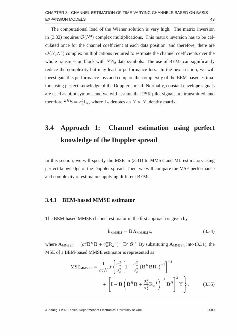
CHAPTER 3. CHANNEL ESTIMATION OF TIME-VARYING CHANNELS BASED ON BASIS
EXPANSION MODELS 43
The computational load of the Wiener solution is very high. The matrix inversion
in (3.32) requiresO(N3) complex multiplications. This matrix inversion has to be cal-
culated once for the channel coefficient at each data position, and therefore, there are
O(NdN4) complex multiplications required to estimate the channel coefficients over the
whole transmission block withNNd data symbols. The use of BEMs can significantly
reduce the complexity but may lead to performance loss. In the next section, we will
investigate this performance loss and compare the complexity of the BEM-based estima-
tors using perfect knowledge of the Doppler spread. Normally, constant envelope signals
are used as pilot symbols and we will assume that PSK pilot signals are transmitted, and
thereforeSHS = σ2sIN , whereIN denotes anN ×N identity matrix.
3.4 Approach 1: Channel estimation using perfect
knowledge of the Doppler spread
In this section, we will specify the MSE in (3.31) to MMSE and ML estimators using
perfect knowledge of the Doppler spread. Then, we will compare the MSE performance
and complexity of estimators applying different BEMs.
3.4.1 BEM-based MMSE estimator
The BEM-based MMSE channel estimator in the first approach is given by
hMMSE,1 = BAMMSE,1z, (3.34)
whereAMMSE,1 = (σ2sB
HB+ σ2nR
−1a )−1BHSH . By substitutingAMMSE,1 into (3.31), the
MSE of a BEM-based MMSE estimator is represented as
MSEMMSE,1 =1
σ2hN
tr
σ2n
σ2s
[
I+σ2n
σ2s
(
BHBRa
)−1]−2
+
[
I−B
(
BHB+σ2n
σ2s
R−1a
)−1
BH
]2
Υ
. (3.35)
J. Zhang, Ph.D. Thesis, Department of Electronics, University of York 2009

CHAPTER 3. CHANNEL ESTIMATION OF TIME-VARYING CHANNELS BASED ON BASIS
EXPANSION MODELS 44
0 2 4 6 8 10 12 14 16 18 20−45
−40
−35
−30
−25
−20
−15
−10
−5
0
Number of basis functions, M
MS
E, d
B
GCEBSDPSKLWiener
Figure 3.2: MSE performance of the BEM-based MMSE channel estimators versus the
number of basis functions,M , with perfect knowledge of the Doppler spread,N = 100,
SNR = 30 dB,νTs = 0.02.
0 5 10 15 20 25 30−40
−35
−30
−25
−20
−15
−10
−5
0
Number of basis funtions, M
MS
E, d
B
GCEBSDPSKLWiener
Figure 3.3: MSE performance of the BEM-based MMSE channel estimators versus the
number of basis functions,M , with perfect knowledge of the Doppler spread,N = 100,
SNR = 30 dB,νTs = 0.05.
J. Zhang, Ph.D. Thesis, Department of Electronics, University of York 2009

CHAPTER 3. CHANNEL ESTIMATION OF TIME-VARYING CHANNELS BASED ON BASIS
EXPANSION MODELS 45
Fig. 3.2 and Fig. 3.3 show the MSE performance of the BEM-basedMMSE channel
estimators for time-variant channels withνTs = 0.02 andνTs = 0.05, respectively. We
setN = 100 and SNR= 30dB. It can be seen that the MSE of the BEM-based MMSE
estimators decrease when more basis functions are applied,and for different BEMs, the
number of basis functions required to achieve the lower bound is different. The MMSE
estimator using BS BEM requires a larger number of basis functions than the others to
provide the same performance. This indicates that the modeling error of the BS BEM is
larger than that of the others. However, the MMSE estimatorsusing all BEMs can achieve
the identical lower bound and when the number of basis functions approachesN , there is
no performance loss. Note that these numerical results are based on (3.35), which match
to the results obtained by simulations in which the MSE of estimated are calculated and
averaged over time variant Rayleigh fading channels generated by using the improved
simulator (2.22) introduced in Chapter 3.
The complexity of the BEM-based estimators depends on the BEM used. The gener-
ation of KL and DPS basis functions requires the knowledge ofthe Doppler spread and
uses the singular value decomposition (SVD) to calculate the eigenvectors of theN ×N
matrixΥ. Therefore, for anyν, the generation of KL and DPS basis functions requires
O(N3) complex multiplications [114]. Note that the matrixBHB for KL or DPS BEM
is anM ×M identity matrix, since the basis functions are orthogonal.
For BS and GCE BEMs, which do not require the knowledge of the Doppler spread,
the basis functions can be precalculated and the matricesB, BHB,(
BHB)−1
BH can be
saved in a memory, and therefore, the complexity of generating basis functions is negli-
gible. Moreover, since the matrixB of the BS BEM is a sparse matrix, the complexity of
the MMSE estimator using BS BEM is lower than that of the estimator using GCE BEM
as shown in Table. 3.1.
Table 3.1 shows the number of complex multiplications required by MMSE estimators
using different BEMs in the first approach, whereq is the order of the B-splines and
K = ⌈4(N−1)M−q
⌉ is the number of non-zero elements in each column of the matrix B of
the BS BEM. It can be seen that the complexity of the MMSE estimators using KL and
DPS BEMs is of the same order. The number of complex multiplications required by the
MMSE estimator using GCE BEM isO(N3) less than that required by estimators using
J. Zhang, Ph.D. Thesis, Department of Electronics, University of York 2009

CHAPTER 3. CHANNEL ESTIMATION OF TIME-VARYING CHANNELS BASED ON BASIS
EXPANSION MODELS 46
Calculation KL DPS BS GCE
B O(N3) O(N3) − −
Ra MN2 +M2N MN2 +M2N MN2 +M2N MN2 +M2N
R−1a O(M3) O(M3) O(M3) O(M3)
V =(
σ2sB
HB+ σ2nR
−1a
)
−1
O(M3) O(M3) O(M3) O(M3)
AMMSE,1 = VBHSH (M2 +M)N (M2 +M)N (q + 1)N + (q + 1)KM (M2 +M)N
aMMSE,1 = AMMSE,1z MN MN MN MN
To estimateNNd channel coefficients MNdN MNdN (q + 1)NdN MNdN
Table 3.1: The number of complex multiplications required by MMSE estimators using
different BEMs in the first approach using perfect knowledge of the Doppler spread.
KL and DPS BEMs. WhenM << N , the termO(N3) dominates in the complexity of
the estimators using KL and DPS BEMs. For this case, the complexity of the MMSE
estimator using the GCE BEM is much lower than that of the estimators using KL and
DPS BEMs. WhenM < 5, the complexity of the MMSE estimators using cubic BS
(q = 3) and GCE BEMs is close. However, whenM increases, the complexity of the
MMSE estimator using the GCE BEM is much higher than that of the estimator using the
BS BEM.
3.4.2 BEM-based ML estimator
The BEM-based ML channel estimator is given by
hML,1 = BAML,1z, (3.36)
whereAML,1 = (BHSHSB)−1BHSH . By substitutingAML,1 into (3.31) and taking
SHS = σ2sIN into account, the MSE of the BEM-based ML estimator is represented
as
MSEML,1 =1
σ2hN
tr
(
I−B(BHB)−1BH)
Υ+σ2n
σ2s
B(
BHB)−1
BH
=1
σ2hN
tr(
I−B(BHB)−1BH)
Υ
+σ2nM
σ2sσ
2hN
(3.37)
= δ2m,ML + δ2s,ML, (3.38)
whereδ2m,ML = 1σ2hN
tr(
I−B(BHB)−1BH)
Υ
andδ2s,ML = σ2nM
σ2sσ
2hN
= MβN
, andβ =σ2hσ2s
σ2n
as the signal-to-noise ratio (SNR). WhenM increases,δ2m,ML reduces butδ2s,ML rises up.
J. Zhang, Ph.D. Thesis, Department of Electronics, University of York 2009

CHAPTER 3. CHANNEL ESTIMATION OF TIME-VARYING CHANNELS BASED ON BASIS
EXPANSION MODELS 47
0 2 4 6 8 10 12 14 16 18 20−45
−40
−35
−30
−25
−20
−15
−10
−5
0
Number of basis functions, M
MS
E, d
B
GCEBSDPSKLMSE
ML
Lower
Figure 3.4: MSE performance of the BEM-based ML channel estimators versus the num-
ber of basis functions,M , with perfect knowledge of the Doppler spread,N = 100, SNR
= 30 dB,νTs = 0.02.
0 5 10 15 20 25 30−40
−35
−30
−25
−20
−15
−10
−5
0
Number of basis functions, M
MS
E, d
B
GCEBSDPSKLLower
Figure 3.5: MSE performance of the BEM-based ML channel estimators versus the num-
ber of basis functions,M , with perfect knowledge of the Doppler spread,N = 100, SNR
= 30 dB,νTs = 0.05.
J. Zhang, Ph.D. Thesis, Department of Electronics, University of York 2009

CHAPTER 3. CHANNEL ESTIMATION OF TIME-VARYING CHANNELS BASED ON BASIS
EXPANSION MODELS 48
For the case with fixedN , νTs and SNR, there is a value ofM , below which, the term
δ2m,ML dominates in MSEML,1 and above whichδ2s,ML dominates in MSEML,1. We call this
the optimal number of basis functions, because, for thisM the ML estimator provides
the best performance. The optimal values ofM for different BEMs can be identified, as
shown in Fig. 3.4 and Fig. 3.5 for the cases withνTs = 0.02 andνTs = 0.05, respectively.
We setN = 100 and SNR to30dB. Note that these numerical results also match to the
simulation results. By comparing Fig. 3.4 and Fig. 3.5 with Fig. 3.2 and Fig. 3.3,
we find that unlike the MMSE estimators, the MSE performance of the BEM-based ML
estimators degrades when the number of basis functions is larger than the optimal value
of M .
Calculation KL DPS BS GCE
B O(N3) O(N3) − −
AML,1 =(
σ2sB
HB)
−1BHSH MN +M2 MN +M2 MN +M2 MN +M2
aML,1 = AML,1z MN MN MN MN
To estimateNNd channel coefficients MNdN MNdN (q + 1)NdN MNdN
Table 3.2: The number of complex multiplications required by ML estimators using dif-
ferent BEMs in the first approach using perfect knowledge of the Doppler spread.
We also investigate the complexity of the BEM-based ML estimators. Table. 3.2
shows the number of complex multiplications required by ML estimators with different
BEMs in the first approach using perfect knowledge of the Doppler spread. By comparing
Table. 3.2 with Table. 3.1, we find that for BS and GCE BEMs, the complexity of the ML
estimator is significantly lower than that of the MMSE estimator, since the ML estimators
do not require the matrixRa. However, the complexity of the ML estimators using KL
and DPS BEMs is still high due to the computational load required for the generation of
basis functions.
The results show that in the first approach, the MMSE estimator outperforms the ML
estimator but requires more complex multiplications. WhenM increases, the MMSE
estimators for all BEMs can provide a good performance close to that of the Wiener
solution. The complexity of the estimators using KL and DPS BEMs is much higher than
that of the estimators using BS and GCE BEMs. Among all BEM-based estimators, the
complexity of the one using BS BEM is the lowest.
J. Zhang, Ph.D. Thesis, Department of Electronics, University of York 2009

CHAPTER 3. CHANNEL ESTIMATION OF TIME-VARYING CHANNELS BASED ON BASIS
EXPANSION MODELS 49
Although the performance of the first approach can be very close to the Wiener solu-
tion, the estimators using KL and DPS are too complicated to be implemented in practice.
Moreover, the assumption of perfectly known Doppler spreadis also impractical. In the
next section, we will investigate the performance and complexity of the second approach
using the maximum Doppler spread and compare them with thoseof the first approach.
3.5 Approach 2: Channel estimation using the maximum
Doppler spread
In practical scenarios, the Doppler spread is not always available. Therefore, in [20], the
maximum Doppler spread,νmax, is suggested to generate the DPS basis functions. This
method can also be applied for the KL BEM. For this approach, the generation of KL
and DPS basis functions depends onνmax. Therefore, like the BS and GCE BEMs, the
KL and DPS basis functions can be precalculated and saved in memory. This method can
significantly reduce the complexity of the estimators usingKL and DPS BEMs, but may
also lead to degradation of the performance due to the mismatch between the maximum
Doppler spread and the real Doppler spread. In this section,we will investigate the de-
crease in the complexity and degradation in the MSE performance of the second approach
compared to the first approach where the Doppler spread is perfectly known.
In the second approach, we can precalculate the mismatched covariance matrixΥ for
the Doppler spreadνmax and save it in memory. Elements ofΥ are calculated as
[Υ]t1,t2 = ρ(t1 − t2), (3.39)
where
ρ(τ) = σ2hJ0(2πνmaxτ). (3.40)
The corresponding mismatched covariance matrix of the expansion coefficients is calcu-
lated by
Ra = (BHB)−1BHΥB(BHB)
−1. (3.41)
For KL and DPS BEMs,B is a matrix containing samples of the basis functions generated
by usingνmax. For BS and GCE BEMs,B = B.
J. Zhang, Ph.D. Thesis, Department of Electronics, University of York 2009
CHAPTER 3. CHANNEL ESTIMATION OF TIME-VARYING CHANNELS BASED ON BASIS
EXPANSION MODELS 50
By applying matrices ofB andRa, the expressions of Wiener solution, MMSE esti-
mator and ML estimators are modified as below.
Mismatched Wiener solution
In the second approach, the mismatched Wiener solution is given by
hW,2 =(
σ2sIN + σ2
nΥ−1)−1
SHz. (3.42)
The MSE of the mismatched Wiener solution is represented as
MSEW,2 =1
σ2hN
tr
Υ−[
2Υ−Υ
(
I+σ2n
σ2s
Υ−1
)(
I+σ2n
σ2s
Υ−1
)−1]
(
I+σ2n
σ2s
Υ−1
)−1
.
(3.43)
BEM-based MMSE estimator
The MMSE channel estimator in the second approach is given by
hMMSE,2 = AMMSE,2z, (3.44)
whereAMMSE,2 =(
σ2sB
HB+ σ2nRa
)−1BHSH , and the MSE is represented as:
MSEMMSE,2 =1
σ2hN
tr
σ2n
σ2s
[
I+σ2n
σ2s
(
BHBRa
)−1]−2
+
[
I− B
(
BHB+σ2n
σ2s
R−1a
)−1
BH
]2
Υ
. (3.45)
BEM-based ML estimator
The ML estimator using in the second approach is given by
hML,2 = AML,2z, (3.46)
whereAML,2 =(
σ2sB
HB)−1
BHSH , and the MSE in represented as
MSEML,2 =1
σ2hN
tr(
I− B(BHB)−1BH)
Υ
+σ2nM
σ2sσ
2hN
. (3.47)
J. Zhang, Ph.D. Thesis, Department of Electronics, University of York 2009

CHAPTER 3. CHANNEL ESTIMATION OF TIME-VARYING CHANNELS BASED ON BASIS
EXPANSION MODELS 51
3.5.1 MSE performance
0.005 0.01 0.015 0.02 0.025 0.03 0.035 0.04 0.045 0.05−44
−43
−42
−41
−40
−39
−38
−37
−36
−35
−34
The normalized Doppler spread νTs
MS
E, d
B
ML2
MMSE2
MMSE1
Figure 3.6: MSE performance of estimators with all BEMs usingthe maximum Doppler
spread,νmaxTs = 0.05,N = 100,M = 26 and SNR = 30dB.
Fig. 3.6 shows the degradation in the MSE performance of the second approach com-
pared with the first approach. We setN = 100, SNR= 30dB andνmaxTs = 0.05. Based
on the results shown in Fig. 3.3, we useM = 26 basis functions to guarantee that all
BEMs provide the best performance forνmaxTs = 0.05. In Fig. 3.6, ML2 and MMSE2
indicate the ML and MMSE estimators in the second approach, respectively, and MMSE1
denotes the MMSE estimators in the first approach. It can be seen that, in the second ap-
proach, the MMSE estimators for all BEMs provide a similar performance as that of the
mismatched Wiener solution usingνmax. In the second approach, the ML estimators using
all BEMs provide a similar performance, which is 3.2dB inferior to that of the MMSE
estimators.
Compared with the performance of MMSE estimators in the first approach, the per-
formance of the MMSE estimator in the second approach degrades whenν significantly
mismatches withνmax. For example, whenν = νmaxTs = 0.05, which indicates that there
is no mismatch, the performance of the MMSE estimator in the second approach is the
J. Zhang, Ph.D. Thesis, Department of Electronics, University of York 2009

CHAPTER 3. CHANNEL ESTIMATION OF TIME-VARYING CHANNELS BASED ON BASIS
EXPANSION MODELS 52
same as that of the MMSE estimators in the first approach. However, whenνTs = 0.01,
the performance of the MMSE estimators usingνmaxTs = 0.05 is 4.2dB inferior to the
performance of the MMSE estimators in the first approach.
3.5.2 Complexity
Calculation KL DPS BS GCE
B − − − −
Ra − − − −
R−1a − − − −
V =(
σ2sB
HB+ σ2nR
−1a
)
−1
O(M3) O(M3) O(M3) O(M3)
AMMSE,2 = VBHSH (M2 +M)N (M2 +M)N (M2 +M)N (M2 +M)N
aMMSE,2 = AMMSE,2z MN MN MN MN
To estimateNNd channel coefficients MNdN MNdN (q + 1)NdN MNdN
Table 3.3: The number of complex multiplications required by MMSE estimators using
different BEMs in the second approach.
Calculation KL DPS BS GCE
B − − − −
AML,2 =(
σ2sB
HB)
−1BHSH MN +M2 MN +M2 MM +M2 MN +M2
aML,2 = AML,2z MN MN MN MN
To estimateNNd channel coefficients MNdN MNdN (q + 1)NdN MNdN
Table 3.4: The number of complex multiplications required by ML estimators using dif-
ferent BEMs in the second approach.
Now, we will investigate the complexity of BEM-based estimators in the second ap-
proach. Table. 3.3 shows the number of complex multiplications required by MMSE
estimators using different BEMs. The matricesB, Υ andR−1a can be precalculated and
saved in memory. Therefore, the estimators with KL and DPS BEMs are significantly
simplified. However, for the estimators using BS and GCE BEMs, the simplification is
not significant. We also find that the MMSE estimators using all BEMs require a similar
number of multiplications whenM < 5. For the case withM > 5, the complexity of the
estimator using the BS BEM is lower than that of the others.
Table. 3.4 shows the number of complex multiplications required by ML estimators
using different BEMs in the second approach. By comparing withTable. 3.2, it can be
seen that the complexity of the ML estimators using KL and DPSBEMs is significantly
J. Zhang, Ph.D. Thesis, Department of Electronics, University of York 2009

CHAPTER 3. CHANNEL ESTIMATION OF TIME-VARYING CHANNELS BASED ON BASIS
EXPANSION MODELS 53
reduced. However, the complexity of the ML estimators usingBS and GCE BEMs is the
same as that of the estimators in the first approach.
The results shown in this section indicate that the use of themaximum Doppler spread
can significantly simplify the estimation when using KL and DPS BEMs. However, for
the estimation using BS and GCE BEMs, the simplification is not significant. Note that
in the second approach, the complexity of the estimator using BS BEM is still the lowest.
The MSE performance of the estimators in the second approachis worse than that of the
estimators in the first approach, especially whenνmax >> ν. In the next section, we will
investigate the third approach using an estimate of the Doppler spread, and compare its
performance and complexity with those of the second approach.
3.6 Approach 3: Channel estimation using an estimate of
the Doppler spread
In this approach, we useν, an estimate of the Doppler spread, to computeRa and generate
the KL and DPS basis functions. The Doppler spread can be estimated based on corre-
lation and variation of channel estimates. For example, in [111], the Doppler estimation
scheme based on the autocorrelation of complex channel estimates is described. Instead
of using channel estimates, the received signal can also be used directly in estimating
Doppler spread information. In [112], the mobile speed is estimated as a function of the
deviation of the averaged signal envelope in flat fading channels. By using the estimate
of the Doppler spread, elements of the estimated covariancematrix,Υ, can be calculated
by
[Υ]t1,t2 = ρ(t1 − t2), (3.48)
where
ρ(τ) = σ2hJ0(2πντ). (3.49)
The estimated covariance matrix of the expansion coefficients is given by
Ra = (BHB)−1BHΥB(BHB)
−1. (3.50)
J. Zhang, Ph.D. Thesis, Department of Electronics, University of York 2009

CHAPTER 3. CHANNEL ESTIMATION OF TIME-VARYING CHANNELS BASED ON BASIS
EXPANSION MODELS 54
For KL and DPS BEMs,B is a matrix containing samples of the basis functions generated
by usingν. For BS and GCE BEMs,B = B.
By applying matricesB andRa, we obtain the MSE for the mismatched Wiener solu-
tion, as well as the MMSE and ML estimators.
Mismatched Wiener solution
The mismatched Wiener solution in the third approach is given by
hW,3 =(
σ2sIN + σ2
nΥ−1)−1
SHz. (3.51)
The MSE of the mismatched Wiener solution is represented as
MSEW,3 =1
σ2hN
tr
Υ−[
2Υ−Υ
(
I+σ2n
σ2s
Υ−1
)(
I+σ2n
σ2s
Υ−1
)−1]
(
I+σ2n
σ2s
Υ−1
)−1
.
(3.52)
BEM-based MMSE estimators
The MMSE channel estimator in the third approach is given by
hMMSE,3 = AMMSE,3z, (3.53)
whereAMMSE,3 =(
σ2sB
HB+ σ2nRa
)−1
BHSH , and the MSE is represented as:
MSEMMSE,3 =1
σ2hN
tr
σ2n
σ2s
[
I+σ2n
σ2s
(
BHBRa
)−1]−2
+
[
I− B
(
BHB+σ2n
σ2s
R−1a
)−1
BH
]2
Υ
. (3.54)
BEM-based ML estimator
The ML estimator in the third approach is given by
hML,3 = AML,3z, (3.55)
J. Zhang, Ph.D. Thesis, Department of Electronics, University of York 2009

CHAPTER 3. CHANNEL ESTIMATION OF TIME-VARYING CHANNELS BASED ON BASIS
EXPANSION MODELS 55
whereAML,3 =(
σ2sB
HB)−1
BHSH , and the MSE is represented as
MSEML,3 =1
σ2hN
tr(
I− B(BHB)−1BH)
Υ
+σ2nM
σ2sσ
2hN
. (3.56)
3.6.1 MSE performance
Generally, an estimate ofν can be represented as
ν = ν +∆ν, (3.57)
where∆ν corresponds to overestimation (∆ν > 0) or underestimation (∆ν < 0) of the
Doppler spread. The sensitivity of the estimators to overestimation and underestimation
is different.
Fig. 3.7 shows the MSE performance of the BEM-based MMSE estimators in the third
appraoch versus∆ν for the case withN = 100, SNR= 30dB, andνTs = 0.02. We set
M = 13. The mismatched Wiener solution and MMSE estimators using all BEMs are
sensitive to underestimation of the Doppler spread (∆ν < 0). In the case of overestima-
tion (∆ν > 0), the performance of the MMSE estimators using BS and GCE BEMs is
similar and close to that of the mismatched Wiener solution.However, the performance
of the MMSE estimators using KL and DPS BEMs degrades when the Doppler spread is
significantly overestimated.
Fig. 3.8 shows the MSE performance of the BEM-based ML estimators in the third
approach versus∆ν for the case withN = 100, SNR= 30dB, andνTs = 0.02. We also
setM = 13. It is seen that the performance of ML estimators using BS and GCE BEMs
is not that significantly affected by∆ν. However, the performance of the ML estimators
using KL and DPS BEMs degrades significantly whenν is underestimated or significantly
overestimated. Therefore, the estimators using BS and GCE BEMsare more robust than
the estimators using KL and DPS BEMs.
In Fig. 3.9, we plot the MSE performance of the MMSE and ML estimation in the
third approach together and find that the MMSE estimators aremore sensitive to under-
estimation of the Doppler spread, but provide better performance than the ML estimators
J. Zhang, Ph.D. Thesis, Department of Electronics, University of York 2009

CHAPTER 3. CHANNEL ESTIMATION OF TIME-VARYING CHANNELS BASED ON BASIS
EXPANSION MODELS 56
−0.02 −0.01 0 0.01 0.02 0.03 0.04 0.05−45
−40
−35
−30
−25
−20
−15
−10
−5
0
∆ ν Ts
MS
E, d
B
GCEBSDPSKLWiener
3
Figure 3.7: MSE performance of MMSE estimators in the third approach versus the
change of the Doppler spread,νTs = 0.02,N = 100,M = 13 and SNR = 30dB.
−0.02 −0.01 0 0.01 0.02 0.03 0.04 0.05−45
−40
−35
−30
−25
−20
−15
−10
−5
0
∆ ν Ts
MS
E, d
B
GCEBSDPSKL
Figure 3.8: MSE performance of ML estimators in the third approach versus the change
of the Doppler spread,νTs = 0.02,N = 100,M = 13 and SNR = 30dB.
J. Zhang, Ph.D. Thesis, Department of Electronics, University of York 2009
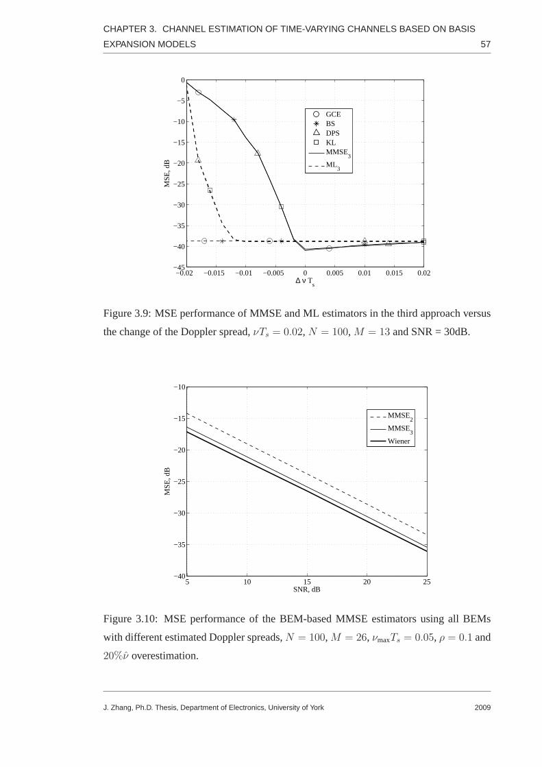
CHAPTER 3. CHANNEL ESTIMATION OF TIME-VARYING CHANNELS BASED ON BASIS
EXPANSION MODELS 57
−0.02 −0.015 −0.01 −0.005 0 0.005 0.01 0.015 0.02−45
−40
−35
−30
−25
−20
−15
−10
−5
0
∆ ν Ts
MS
E, d
B
GCEBSDPSKLMMSE
3
ML3
Figure 3.9: MSE performance of MMSE and ML estimators in the third approach versus
the change of the Doppler spread,νTs = 0.02,N = 100,M = 13 and SNR = 30dB.
5 10 15 20 25−40
−35
−30
−25
−20
−15
−10
SNR, dB
MS
E, d
B
MMSE2
MMSE3
Wiener
Figure 3.10: MSE performance of the BEM-based MMSE estimators using all BEMs
with different estimated Doppler spreads,N = 100,M = 26, νmaxTs = 0.05, ρ = 0.1 and
20%ν overestimation.
J. Zhang, Ph.D. Thesis, Department of Electronics, University of York 2009
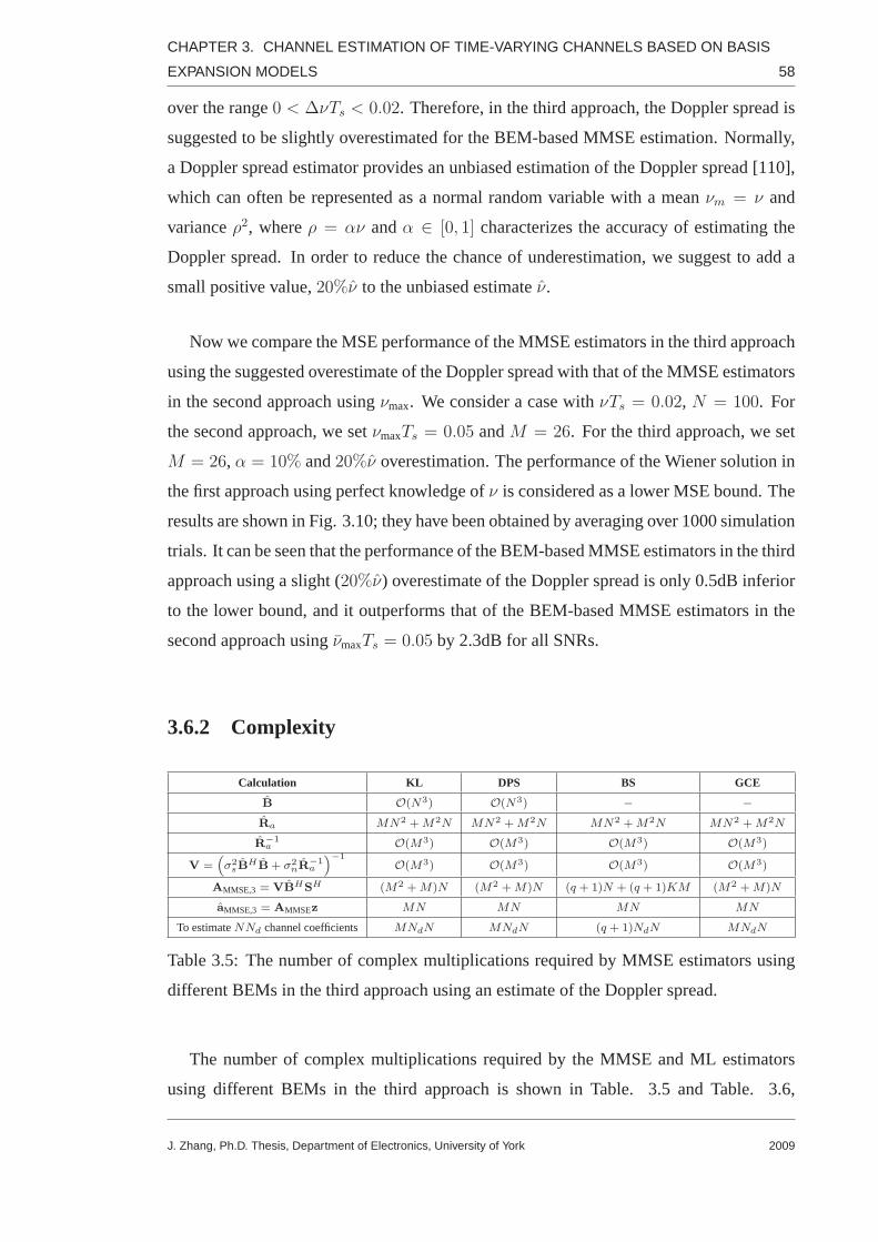
CHAPTER 3. CHANNEL ESTIMATION OF TIME-VARYING CHANNELS BASED ON BASIS
EXPANSION MODELS 58
over the range0 < ∆νTs < 0.02. Therefore, in the third approach, the Doppler spread is
suggested to be slightly overestimated for the BEM-based MMSE estimation. Normally,
a Doppler spread estimator provides an unbiased estimationof the Doppler spread [110],
which can often be represented as a normal random variable with a meanνm = ν and
varianceρ2, whereρ = αν andα ∈ [0, 1] characterizes the accuracy of estimating the
Doppler spread. In order to reduce the chance of underestimation, we suggest to add a
small positive value,20%ν to the unbiased estimateν.
Now we compare the MSE performance of the MMSE estimators in the third approach
using the suggested overestimate of the Doppler spread withthat of the MMSE estimators
in the second approach usingνmax. We consider a case withνTs = 0.02, N = 100. For
the second approach, we setνmaxTs = 0.05 andM = 26. For the third approach, we set
M = 26, α = 10% and20%ν overestimation. The performance of the Wiener solution in
the first approach using perfect knowledge ofν is considered as a lower MSE bound. The
results are shown in Fig. 3.10; they have been obtained by averaging over 1000 simulation
trials. It can be seen that the performance of the BEM-based MMSE estimators in the third
approach using a slight (20%ν) overestimate of the Doppler spread is only 0.5dB inferior
to the lower bound, and it outperforms that of the BEM-based MMSE estimators in the
second approach usingνmaxTs = 0.05 by 2.3dB for all SNRs.
3.6.2 Complexity
Calculation KL DPS BS GCE
B O(N3) O(N3) − −
Ra MN2 +M2N MN2 +M2N MN2 +M2N MN2 +M2N
R−1a O(M3) O(M3) O(M3) O(M3)
V =(
σ2sB
HB+ σ2nR
−1a
)
−1
O(M3) O(M3) O(M3) O(M3)
AMMSE,3 = VBHSH (M2 +M)N (M2 +M)N (q + 1)N + (q + 1)KM (M2 +M)N
aMMSE,3 = AMMSEz MN MN MN MN
To estimateNNd channel coefficients MNdN MNdN (q + 1)NdN MNdN
Table 3.5: The number of complex multiplications required by MMSE estimators using
different BEMs in the third approach using an estimate of the Doppler spread.
The number of complex multiplications required by the MMSE and ML estimators
using different BEMs in the third approach is shown in Table. 3.5 and Table. 3.6,
J. Zhang, Ph.D. Thesis, Department of Electronics, University of York 2009

CHAPTER 3. CHANNEL ESTIMATION OF TIME-VARYING CHANNELS BASED ON BASIS
EXPANSION MODELS 59
Calculation KL DPS BS GCE
B O(N3) O(N3) − −
AML,3 =(
σ2sB
HB
)
−1
BHSH MN +M2 MN +M2 MN +M2 MN +M2
aML,3 = AML,3z MN MN MN MN
To estimateNNd channel coefficients MNdN MNdN (q + 1)NdN MNdN
Table 3.6: The number of complex multiplications required by ML estimators using dif-
ferent BEMs in the third approach using an estimate of the Doppler spread.
respectively. It is clear that the complexity of the third approach is the same as that of
the first approach. The complexity of the estimators using KLand DPS BEMs in the
third approach is much higher than that of the estimators in the second approach. For the
estimation using BS and GCE BEMs in the third approach, the complexity is close to that
of the estimation in the second approach.
By comparing the third approach using a slight (20%ν) overestimate of the Doppler
spread with the second approach using the maximum Doppler spread, we find that al-
though the complexity of the second approach is lower, its performance is worse than that
of the third approach. Moreover, the increase of the complexity in the third approach is
only significant for the estimation using KL and DPS BEMs. For the estimation using
BS and GCE BEMs, the complexity of the third approach is close to that of the second
approach. It is also worthy to emphasize that the complexityof the estimators using BS
BEM is the lowest in all approaches. Therefore, the BS BEM is the most practical choice
due to its highest robustness and lowest complexity.
3.7 Conclusions
In this chapter, BEM-based estimators for time-variant fading channels have been inves-
tigated. The MSE of a generic linear channel estimator with linearly independent BEMs
has been derived. We have investigated and compared the MSE performance and com-
plexity for three approaches using different BEMs, such as KL, DPS, GCE and BS BEMs
for estimation with perfect or inaccurate knowledge of the Doppler spread:
1) channel estimation using perfect knowledge of the Doppler spread;
J. Zhang, Ph.D. Thesis, Department of Electronics, University of York 2009

CHAPTER 3. CHANNEL ESTIMATION OF TIME-VARYING CHANNELS BASED ON BASIS
EXPANSION MODELS 60
2) channel estimation using the maximum Doppler spread as suggested in [20];
3) channel estimation with an estimate of the Doppler spread.
In the first approach based on the impractical assumption of perfect knowledge of the
Doppler spread, when the number of basis functions increases, all BEM-based MMSE
estimators can provide a similar performance close to that of the Wiener solution. How-
ever, the performance of the ML estimator degrades after an optimal number of basis
functions. Although the B-splines require slightly more basis functions than the other
BEMs to achieve the same estimation performance, the complexity of the estimator using
B-splines is still lower than that of the others.
In the second approach, the maximum Doppler spread is used tocalculate the fading
statistics and generate the KL and DPS basis functions. Although the estimation is sim-
plified with respect to the first approach, the significant mismatch between the maximum
Doppler spread and the real Doppler spread leads to degradation in the MSE performance.
Moreover, the decrease of the complexity is only significantfor the estimation using KL
and DPS BEMs, but not significant for the estimation using BS andGCE BEMs.
The third approach uses an estimate of the Doppler spread to compute the fading statis-
tics and generate the KL and DPS basis functions. In this approach, all estimators are
sensitive to underestimation of the Doppler spread but may have little sensitivity to over-
estimation depending on the BEM used. The estimators using BS and GCE BEMs are
more robust than the estimators using KL and DPS BEMs. The estimation in this ap-
proach using a slight (20%) overestimate of the Doppler spread outperforms the estima-
tion in the second approach using the maximum Doppler spread. The MSE performance
of the MMSE estimation in the third approach is very close to the performance of the
Wiener solution with perfect knowledge of the Doppler spread. In this approach, the esti-
mation with KL and DPS BEMs is more complicated than those in the second approach.
However, the increase of complexity for the estimation using BS and GCE BEMs in this
approach is close to that in the second approach.
It is also worthy to emphasize that the complexity of the estimation using BS BEM
is the lowest in each approach. Therefore, the BS-based estimation using a slight (e.g.,
20%) overestimate of the Doppler spread is a good practical choice providing a good
J. Zhang, Ph.D. Thesis, Department of Electronics, University of York 2009
CHAPTER 3. CHANNEL ESTIMATION OF TIME-VARYING CHANNELS BASED ON BASIS
EXPANSION MODELS 61
performance, high robustness and low complexity.
In the following chapters, we will investigate the best performance that can be obtained
by using the optimal detection with imperfect channel estimation. Therefore, we will
assume that the Doppler spread is perfectly known. Moreover, the cubic BS BEM will be
used to approximate the time-variant channels.
J. Zhang, Ph.D. Thesis, Department of Electronics, University of York 2009
Chapter 4
Optimal and Mismatched Detection in
SISO Frequency-Flat Fading Channels
with Imperfect Channel Estimation
Contents
4.1 Introduction . . . . . . . . . . . . . . . . . . . . . . . . . . . . . . . 62
4.2 Transmission model . . . . . . . . . . . . . . . . . . . . . . . . . . . 64
4.3 Generic optimal detection . . . . . . . . . . . . . . . . . . . . . . . . 65
4.4 Generic mismatched detection . . . . . . . . . . . . . . . . . . . . . 67
4.5 Optimal and mismatched detection in time invariant SISO channels 69
4.6 Optimal and mismatched detection in SISO time variant channels . 70
4.7 Simulation results . . . . . . . . . . . . . . . . . . . . . . . . . . . . 77
4.8 Conclusions . . . . . . . . . . . . . . . . . . . . . . . . . . . . . . . . 84
4.1 Introduction
In communication systems transmitting data through unknown channels, traditional de-
tection techniques are based on channel estimation (e.g., by using pilot signals), and then
J. Zhang, Ph.D. Thesis, Department of Electronics, University of York
62
2009

CHAPTER 4. OPTIMAL AND MISMATCHED DETECTION IN SISO FREQUENCY-FLAT
FADING CHANNELS WITH IMPERFECT CHANNEL ESTIMATION 63
treating the estimates as perfect in a minimum distance detector; we call such detectors
mismatched(after [35]). A better detection performance can be obtained in anoptimal
detector that does not estimate the channel explicitly but jointly processes the received
pilot and data symbols to recover the data [35]. The optimal detector in [35] was obtained
for communication scenarios with space-time coding in a channel with uncorrelated fad-
ing and additive white noise. In this chapter, we consider a more general scenario that is
applicable to channels with correlated fading. We derive the generic optimal detector and
specify it for frequency-flat fading channels. We then compare its detection performance
with that of mismatched detectors using different channel estimation techniques for both
cases of time-invariant and time-variant fading.
In time-variant fading channels, the channel estimation isdifficult, especially in sys-
tems with powerful channel codes, such as turbo codes, generally operating at low SNR
where pilot-based channel estimates are often of low accuracy. Iterative channel esti-
mation and decoding over flat fading channels has been proposed to improve the esti-
mates [63, 115]. In this chapter, we will consider representation of channel gain time
variations by using basis functions. As shown in Chapter 3, compared with the other
BEMs, the B-splines provide high accuracy of approximation and require lower complex-
ity. Therefore, we consider approximation of the channel time variations by B-splines,
and, for this case, investigate the detection performance of the optimal detector. We then
investigate iterative receivers that exchange channel anddata estimates in a system trans-
mitting turbo-encoded data. Four channel estimation schemes are considered: the ML
estimator, MMSE estimator, regularized ML estimator, and an estimator providing statis-
tics for the optimal detector.
This chapter is organized as follows. In Section 4.2, the transmission model is in-
troduced. The generic optimal detection and mismatched detection are derived and de-
scribed in Section 4.3 and Section 4.4, respectively. In Section 4.5, the optimal detector is
specified for time-invariant channels. Section 4.6 specifies the optimal detector for time-
variant fading channels approximated by B-splines and describes iterative receivers with
soft-input hard-output and/or soft-input soft-output turbo decoding scheme. Numerical
results are given in Section 4.7. Section 4.8 concludes the chapter.
J. Zhang, Ph.D. Thesis, Department of Electronics, University of York 2009

CHAPTER 4. OPTIMAL AND MISMATCHED DETECTION IN SISO FREQUENCY-FLAT
FADING CHANNELS WITH IMPERFECT CHANNEL ESTIMATION 64
4.2 Transmission model
We assume that the data transmission is split into two parts,pilot and data transmission.
For the pilot transmission, the received signal is modeled as
zp = Ψpa+ np (4.1)
wherezp is anNp × 1 received signal vector andΨp is anNp ×M matrix formed from
pilot symbols (for time-invariant channels) or formed fromthe multiplication of pilot
symbols and basis functions (for time-variant channels). TheNp × 1 complex-valued
noise vectornp has a zero mean Gaussian PDFNC(0,Rp) with covariance matrixRp =
EnpnHp . The vectora = [a1, . . . , aM ]T is anM × 1 vector of complex-valued channel
gains (for time-invariant channels) or basis coefficients (for time-invariant channels) with
the Gaussian PDF
f(a) = NC(0,Ra) (4.2)
whereRa = EaaH is anM × M covariance matrix. The functionf(a) defines a
Rayleigh fading channel. The definition of the vectora depends on the considered chan-
nel. In time-invariant channels,a contains the channel gains, i.e.,a = h, and in time-
variant channels,a contains the expansion coefficients, i.e.,a = [a1, . . . , aM ]H . Cor-
respondingly, the structure ofΨp and is modified. In time-invariant channels,Ψp =
sp = [sp(1), . . . , sp(i), . . . , sp(Np)]H wheresp(i) is an transmitted pilot symbols. In time-
variant channels,Ψp andΨd become matrices as
Ψp = DpBp, (4.3)
whereDp being a diagonal matrix defined as
Dp = diagsp(t1), . . . , sp(tNp), (4.4)
The matricesBp contain samples of the basis functions at the pilot instants. The de-
tails will be introduced in section 4.5 and section 4.6.1 corresponding to time-invariant
channels and time-variant channels, respectively.
The PDF of the received signal vectorzp for a given vectora is
p(zp|a) = NC(Ψpa,Rp). (4.5)
J. Zhang, Ph.D. Thesis, Department of Electronics, University of York 2009

CHAPTER 4. OPTIMAL AND MISMATCHED DETECTION IN SISO FREQUENCY-FLAT
FADING CHANNELS WITH IMPERFECT CHANNEL ESTIMATION 65
For the data transmission, the received signal is modeled as
zd = Ψda+ nd (4.6)
wherezd is the receivedNd × 1 data vector andΨd is anNd × M matrix which de-
pends on a vectord of transmitted data symbols. In time-variant channels,Ψd =
[d(1), . . . , d(i), . . . , d(Nd)]H whered(i) is an transmitted data symbol, andΨd = DdBd,
whereDd = diagd1, . . . , dNd andBd contains samples of the basis functions at the data
instants. TheNd × 1 noise vectornd has the Gaussian PDFNC(0,Rd) with covariance
matrix Rd = EndnHd . The PDF of the vectorzd for given vectorsd anda is also
Gaussian:
p(zd|d, a) = NC(Ψda,Rd). (4.7)
The transmission model presented in (4.1) and (4.6) is quitegeneral. It can be used to
describe single-input single-output or multi-input multi-output systems in both frequency-
flat and frequency-selective fading channels or in time invariant or variant channels. For
different channels, the structure of matrices or vectors defined above, i.e.,Ψd, Ψp, zp, zd
anda should be modified. The modifications of these matrices and vectors corresponding
are declared in following chapters corresponding to different channels considered.
4.3 Generic optimal detection
For the described transmission model, the optimal detectoris derived by maximizing the
PDFp(zd|d, zp) of the signalzd received at the data stage, conditioned on the transmitted
symbolsd and the signalzp received at the pilot stage, over the data set (alphabet)A:
dopt = argmaxd∈A
p(zd|d, zp)
= argmaxd∈A
ln [p(zd|d, zp)] . (4.8)
In the case of QAM transmission, the alphabetA includes all symbols corresponding to
the QAM constellation points. The PDFp(zd|d, zp) is obtained from the PDFp(zd|d, a)in (4.7) by integrating out the channel parametersa which are now treated asnuisance
parameters:
p(zd|d, zp) =∫
p(zd|d, a)f(a|zp)da (4.9)
J. Zhang, Ph.D. Thesis, Department of Electronics, University of York 2009

CHAPTER 4. OPTIMAL AND MISMATCHED DETECTION IN SISO FREQUENCY-FLAT
FADING CHANNELS WITH IMPERFECT CHANNEL ESTIMATION 66
where theposteriorPDF f(a|zp) of channel parameters is conditioned on the received
pilot signalzp. Since (4.1) is theBayesian general linear model, the PDFf(a|zp) is also
Gaussian (see [113], pp.326),
f(a|zp) = NC(ma,Sa), (4.10)
with meanma and covarianceSa given by
ma = (Γp +R−1a )−1Lp, (4.11)
Sa = (Γp +R−1a )−1, (4.12)
where
Lp = ΨHp R
−1p zp, (4.13)
Γp = ΨHp R
−1p Ψp. (4.14)
If Rp = σ2nINp
(i.e., the noise is white with varianceσ2n), then we have
Lp = σ−2n ΨH
p zp, (4.15)
Γp = σ−2n ΨH
p Ψp, (4.16)
whereINpdenotes anNp ×Np identity matrix.
By substituting (4.7) in (4.9), we obtain
p(zd|d, zp) = c3
∫
e2ℜ(aHLd)−aHΓdaf(a|zp)dℜ(a)dℑ(a) (4.17)
whereℜ(·) denotes the real part andℑ(·) denotes the imaginary part,
c3 =1
πNd|Rd|e−zH
dR
−1
dzd > 0
is a constant, and|Rd| denotes the determinant of the matrixRd. By substituting (4.10)
in (4.17) and taking into account (7.3) in Appendix A, we obtain
p(zd|d, zp) =c3
|SaΓd + IM | exp
(Ld + Lp)H(Γd + S−1
a)−1(Ld + Lp)
(4.18)
=c3
|SaΓd + IM | exp
2ℜ[LHd (SaΓd + IM)−1ma] + LHd (SaΓd + IM)−1SaLd
−mHaΓd(SaΓd + IM)−1ma
(4.19)
where
Ld = ΨHd R
−1d zd, (4.20)
Γd = ΨHd R
−1d Ψd. (4.21)
J. Zhang, Ph.D. Thesis, Department of Electronics, University of York 2009

CHAPTER 4. OPTIMAL AND MISMATCHED DETECTION IN SISO FREQUENCY-FLAT
FADING CHANNELS WITH IMPERFECT CHANNEL ESTIMATION 67
For the white noise case, we haveRd = σ2nINd
and
Ld = σ−2n ΨH
d zd, (4.22)
Γd = σ−2n ΨH
d Ψd. (4.23)
Finally, the optimal detector (4.8) is given by
dopt = argmind∈A
λ(d) . (4.24)
where the metricλ(d) to be minimized is given by
λ(d) = −(Ld + Lp)H(Γd + Γp +R−1
a )−1(Ld + Lp) + ln |Γd + Γp +R−1a | (4.25)
= ln |SaΓd + IM | − 2ℜ[LHd (SaΓd + IM)−1ma]− LHd (SaΓd + IM)−1SaLd
+mHaΓd(SaΓd + IM)−1ma. (4.26)
The first presentation (4.25) of the optimal metricλ(d) shows how this metric is ex-
pressed in terms of the channel statisticLp, which is a vector of outputs of filters matched
to the pilot signals, and the correlation matrixΓp of the pilot signals. The second pre-
sentation (4.26) shows how the optimal metric is expressed in terms of the meanma and
covarianceSa of the posterior PDFf(a|zp).
If the perfect channel information (PCI) is available, we canwrite ma = a andSa =
0M , where0M is anM ×M zero matrix. In this case, the metric (4.26) takes the form
λ(d) = −2ℜ(LHd a) + aHΓda. (4.27)
The detector minimizing the metric (4.27) is equivalent to the classical minimum distance
detector
dPCI = argmind∈A
||zd −Ψda||2R−1
d
. (4.28)
In what follows, we will only consider scenarios with additive white noise.
4.4 Generic mismatched detection
The vectorma in (4.11) is known to be the MMSE estimate of the channel parametersa,
i.e.,
aMMSE = ma, (4.29)
J. Zhang, Ph.D. Thesis, Department of Electronics, University of York 2009

CHAPTER 4. OPTIMAL AND MISMATCHED DETECTION IN SISO FREQUENCY-FLAT
FADING CHANNELS WITH IMPERFECT CHANNEL ESTIMATION 68
and this estimate is unbiased and has the covariance matrixSa (4.12) [113]. At high SNR,
i.e.,σ2n → 0, we obtain
f(a|zp) → δ(a−ma), (4.30)
whereδ(a−ma) is an analog of the Dirac delta function for a vector argument. Then the
integration in (4.9) results in
p(zd|d, zp) → p(zd|d, a = aMMSE), (4.31)
and the optimal detector (4.8) becomes a mismatched detector where the MMSE channel
estimates
aMMSE = (Γp +R−1a Lp (4.32)
are treated as perfect when minimizing the Euclidean distance:
dMMSE = argmind∈A
(zd −ΨdaMMSE)H(zd −ΨdaMMSE)
. (4.33)
This motivates us to compare the optimal detector with the MMSE-mismatched detec-
tor. The mismatched detector with MMSE channel estimates exploits the samea priori
information as the optimal detector, but, in a different way. It minimizes the error of
channel estimates, while the optimal detector minimizes the probability of detection er-
rors. Therefore, when comparing the detection performanceof the two detectors, we
expect the optimal detector to outperform the mismatched detector with MMSE channel
estimates.
The optimal detector and mismatched detector with MMSE channel estimates require
the knowledge of the fading statistics that are not always available. Therefore, it is of
interest to consider the mismatched detector with ML channel estimates
dML = argmaxd∈A
(zd −ΨdaML )H(zd −ΨdaML )
(4.34)
where the ML channel estimates are given by
aML = (ΨHp Ψp)
−1ΨHp zp = Γ−1
p Lp. (4.35)
When comparing (4.32) and (4.35), it is seen that the inverse of the fading covariance ma-
trix Ra in (4.32) plays a regularization role. This, however, requires the fading covariance
to be known. Therefore, we will also consider a mismatched detector
dǫ = argmaxd∈A
(zd −Ψdaǫ)H(zd −Ψdaǫ)
(4.36)
J. Zhang, Ph.D. Thesis, Department of Electronics, University of York 2009

CHAPTER 4. OPTIMAL AND MISMATCHED DETECTION IN SISO FREQUENCY-FLAT
FADING CHANNELS WITH IMPERFECT CHANNEL ESTIMATION 69
with channel estimates using regularization based on the diagonal loading
aǫ = (Γp + ǫIM)−1Lp (4.37)
whereǫ ≥ 0 is a regularization parameter. Such regularization does not require the fading
statistics to be available. Note that forǫ = 0, we haveaǫ = aML .
Thus, we are going to investigate the detection performanceof the following detectors:
1) optimal detector defined by (4.24) and (4.25);
2) mismatched detector with MMSE channel estimates given by(4.33);
3) mismatched detector with ML channel estimates given by (4.34); and
4) mismatched detector withǫ-ML channel estimates given by (4.36).
The relationship (4.24) describes the optimal detector applicable to many communi-
cations scenarios. However, in this chapter we are only interested in investigating single-
user systems in SISO frequency-flat time-invariant and time-variant Rayleigh fading chan-
nels.
4.5 Optimal and mismatched detection in time invariant
SISO channels
In this section, we specify the optimal detector for time-invariant fading channels with
QAM transmission and show that for signals with constant envelope the mismatched de-
tectors are optimal.
Consider the transmission in a SISO time invariant channel, described as
zp = hsp + np (4.38)
zd = hsd + nd (4.39)
i.e.,M = 1, a = h is a complex-valued scalar,Ra = σ2h = E|h|2, andΨp = sp is a
Np × 1 vector of pilot symbols. We consider symbol-by-symbol detection, i.e.,Nd = 1
J. Zhang, Ph.D. Thesis, Department of Electronics, University of York 2009

CHAPTER 4. OPTIMAL AND MISMATCHED DETECTION IN SISO FREQUENCY-FLAT
FADING CHANNELS WITH IMPERFECT CHANNEL ESTIMATION 70
andΨd = d. We only consider the white noise case, i.e.,Rd = σ2n andRp = σ2
nINp.
Denoteη = σ2a/σ
2n, γp = sHp zp, andγd = d∗zd. Then, from (4.12) and (4.11), we obtain
Sa = σ2a(Epη + 1)−1 andma = ηγp(Epη + 1)−1, whereEp = sHp sp is the energy of the
pilot signal. We also obtainLp = γpσ−2n , Γp = Epσ
−2n , Ld = γdσ
−2n , andΓd = |d|2σ−2
n .
With these notations, from (4.25) we arrive at the optimal detector
dopt = argmaxd∈A
|d∗zd + γp|2σ2n(|d|2 + Ep + 1/η)
− ln
(
|d|2 + Ep +1
η
)
. (4.40)
For signals with constant envelope|d| = const, such as PSK signals, from (4.40) we
obtain
dopt = argmaxd∈A
ℜ(γ∗pγd)
= dML = dMMSE = dǫ. (4.41)
The data symbol estimate (4.41) is equivalent to the mismatched detectors with the fol-
lowing estimates of the channel gain:
aML = γp/Ep, (4.42)
aMMSE = γp/(Ep + 1/η), (4.43)
aǫ = γp/(Ep + σ2n), (4.44)
correcting the received signal according to these estimates (z0 = a∗MLzd or z0 = a∗MMSEzd
or z0 = a∗ǫzd), and, finally, deciding on the transmitted symbold by mappingz0 to the PSK
constellationA. Thus, for constant envelope signals (such as PSK signals) all the three
mismatched detectors are optimal. In other cases of QAM signals, the optimal detector is
given by (4.40).
4.6 Optimal and mismatched detection in SISO time
variant channels
4.6.1 Transmission model
Now we consider single-user transmission in time variant channels. We assume that a
data block ofN symbols is transmitted,Np of which are pilot symbols and the other
J. Zhang, Ph.D. Thesis, Department of Electronics, University of York 2009

CHAPTER 4. OPTIMAL AND MISMATCHED DETECTION IN SISO FREQUENCY-FLAT
FADING CHANNELS WITH IMPERFECT CHANNEL ESTIMATION 71
Figure 4.1: Structure of the transmitted data block.
Nd = N −Np are data symbols as shown in Fig. 4.1. The received signal corresponding
to the pilot and data parts of the data block are modeled, respectively, as
zp(tk) = sp(tk)h(tk) + n(tk), k = 1, . . . , Np, (4.45)
zd(τk) = sd(τk)h(τk) + n(τk), k = 1, . . . , Nd, (4.46)
wheresd(τk) = dk is a data symbol transmitted at timeτk, n(t) is the noise, andh(t)
states a Rayleigh fading channel following Jakes’ model [50,51]. The covariance matrix
of such fading channels is anN ×N matrix with elements
[Υ]t1,t2 = ρ(t1 − t2), (4.47)
wheret1, t2 = 1, . . . , N , andρ(τ) is the autocorrelation function of Jakes’ fading process
[50] as shown by (3.4) in Chapter 3
ρ(τ) = σ2hJ0(2πντ), (4.48)
σ2h is the variance of the channel coefficients,J0(·) is the zero-order Bessel function of
the first kind,ν is the Doppler frequency.
As shown in Chapter 3, BEMs can be used to approximate the time-variant fading
channels following Jakes’ model. With a BEM, the task of estimatingN time variant
channel gains transforms to estimating onlyM time invariant expansion coefficients,
whereM << N , and the time-varying channel is represented as a series
h(t) =M∑
m=1
amϕm(t), t = 0, . . . , N − 1, (4.49)
J. Zhang, Ph.D. Thesis, Department of Electronics, University of York 2009

CHAPTER 4. OPTIMAL AND MISMATCHED DETECTION IN SISO FREQUENCY-FLAT
FADING CHANNELS WITH IMPERFECT CHANNEL ESTIMATION 72
whereϕm(t)Mm=1 are basis functions. In the matrix form, (4.49) can be represented by
h = Ba, (4.50)
whereB is anN × M matrix with elements[B]t,m = ϕm(t), t = 0, . . . , N − 1, and
a = [a1, . . . , am, . . . , aM ]T is anM×1 vector corresponding to the expansion coefficients.
We can represent the received data and pilot signals in the matrix form (4.1) and (4.6),
respectively, with
Ψp = DpBp, Ψd = DdBd, (4.51)
andDp andDd being diagonal matrices defined as
Dp = diagsp(t1), . . . , sp(tNp), (4.52)
Dd = diagd1, . . . , dNd. (4.53)
The matricesBp andBd contain samples of the basis functions at the pilot and data
symbol instants, respectively:
[Bp]k,m = ϕm(tk), [Bd]k,m = ϕm(τk). (4.54)
Using these notations, and denoting
βd = DHd zd, βp = DH
p zp (4.55)
and
Fd = DHd Dd, Fp = DH
p Dp, (4.56)
we obtain:
Ld = σ−2n BH
d βd, Lp = σ−2n BH
p βp, (4.57)
and
Γd = σ−2n BH
d FdBd, Γp = σ−2n BH
p FpBp. (4.58)
4.6.2 Optimal detection
The optimal detector becomes very complicated for highNd. We want to consider the
simplest case of symbol-by-symbol detection of data symbols in a data block. In this
J. Zhang, Ph.D. Thesis, Department of Electronics, University of York 2009
CHAPTER 4. OPTIMAL AND MISMATCHED DETECTION IN SISO FREQUENCY-FLAT
FADING CHANNELS WITH IMPERFECT CHANNEL ESTIMATION 73
case, expressions above are simplified:Dd = d, Fd = |d|2 andβd = d∗zd are now
scalars;Bd is a(1×M) vector whose elements are values of the basis functions at the data
symbol instant;Ld = σ−2d∗zdBHd ; andΓd = σ−2|d|2BH
d Bd. The optimal detector (4.24)
minimizes the metricλ(d) which is now given by
λ(d) = − 1
σ2n
(
BHd βd +BH
p βp)H (|d|2BH
d Bd +BHp FpBp + σ2
nR−1a
)−1
×(
BHd βd +BH
p βp)
+ ln∣
∣|d|2BHd Bd +BH
p FpBp + σ2nR
−1a
∣
∣ . (4.59)
The optimal detector based on modeling time-variant fadingusing a BEM requires an
explicit expression for the fading covarianceRa. To obtainRa, we can use the transform
(3.25)
Ra = (BHB)−1BHΥB(BHB)−1. (4.60)
If the perfect channel information is available, for the PDFf(a|zp) = NC(ma,Sa) we
can writema = a andSa = 0M . In this case, the optimal metric (4.59) takes the form
λ(d) = −2ℜ(LHd a) + aHΓda. The detector minimizing this metric is equivalent to the
classical minimum distance detector
dPCI = argmind∈A
(zd −Ψda)H(zd −Ψda)
. (4.61)
4.6.3 Mismatched detection
As introduced above, we will consider the mismatched detectors using MMSE, ML and
ǫ-ML channel estimates and compare their performance with that of the optimal detector.
Since we have used a BEM to approximate time-variant channelshere, and therefore, the
task of the channel estimator becomes to estimateM expansion coefficients. The MMSE
channel estimates are given by
aMMSE = (BHp FpBp + σ2
nR−1a)−1BH
p DHp zp. (4.62)
Correspondingly, a mismatched detector that treatsaMMSE as perfect and minimizes the
Euclidean distance is represented as
dMMSE = argmind∈A
(zd −ΨdaMMSE)H(zd −ΨdaMMSE)
. (4.63)
J. Zhang, Ph.D. Thesis, Department of Electronics, University of York 2009

CHAPTER 4. OPTIMAL AND MISMATCHED DETECTION IN SISO FREQUENCY-FLAT
FADING CHANNELS WITH IMPERFECT CHANNEL ESTIMATION 74
The ML channel estimates are given by
aML = (BHp FpBp)
−1BHp D
Hp zp. (4.64)
and a mismatched detector applying the ML channel estimatesis represented as
dML = argmind∈A
(zd −ΨdaML )H(zd −ΨdaML )
(4.65)
Theǫ-ML channel estimates are given by
aǫ = (BHp FpBp + ǫσ2
nIM)−1BHp D
Hp zp, (4.66)
whereǫ ≥ 0 is a regularization parameter andIM denotes anM ×M identity matrix.
Such regularization does not require the fading statisticsto be available. A mismatched
detector using theǫ-ML estimates is represented as
dǫ = argmind∈A
(zd −Ψdaǫ)H(zd −Ψdaǫ)
. (4.67)
Note that forǫ = 0, we haveaML = aǫ. It can be shown that theǫ-ML channel estimate
provides the minimum MSE ifǫ = σ−2a ; this value ofǫ is used in our simulations.
4.6.4 Iterative receivers
Figure 4.2: Transmitter.
The transmission system with QAM modulation is shown in Fig .4.2. In the trans-
mitter, information bits are firstly encoded by a turbo encoder of 1/3 rate with generator
polynomials [013,015] in octal notation. The output bits ofthe turbo encoder are channel-
interleaved and grouped into QAM symbols. Then, pilot symbols are inserted periodically
every(P − 1) data symbols as shown in Fig. 4.1.
Fig. 4.3 or Fig. 4.4 show the structure of soft-input hard-output (SIHO) or soft-input
soft-output (SISO) turbo decoders, respectively.
J. Zhang, Ph.D. Thesis, Department of Electronics, University of York 2009

CHAPTER 4. OPTIMAL AND MISMATCHED DETECTION IN SISO FREQUENCY-FLAT
FADING CHANNELS WITH IMPERFECT CHANNEL ESTIMATION 75
The receiver applying SIHO turbo decoder (Fig. 4.3) recovers the transmitted coded
bits by applying a turbo encoder same as the one used in the transmitter to encoding the
hard output of the decoder. The soft metrics output from the detector are de-interleaved
and then passed to a turbo decoder. The SIHO turbo decoder in Fig. 4.3 outputs the
decoded bits which are then turbo encoded. This receiver is too complicated for practical
scenarios, and moreover, its performance is much worse thanthat of the iterative receiver
with SISO Turbo decoder as shown in following simulations.
The receiver applying SISO turbo decoder (Fig. 4.4) performs several iterations, in
which channel estimation and decoding are refined. The receiver uses an SISO turbo
decoder. For every bitck = ±1 of a received symbol,k = 1, . . . , K, the a posteriori
log-likelihood ratio (LLR) is computed as [116,117]
λck = ln
[∑
d∈A+
ke−λ(d)
∏
i 6=k P (ci)∑
d∈A−
ke−λ(d)
∏
i 6=k P (ci)
]
, (4.68)
where thea priori probabilityP (ci) of a symbol bit is expressed in terms of itsa priori
LLR L(ci) [118]:
P (ci) =1
2
[
1 + ci tanh
(
1
2L(ci)
)]
,
A±k = d ∈ A|ck = ±1, and the metricλ(d) depends on the detector used. For the first
iteration, we have
λck = ln∑
d∈A+
k
e−λ(d) − ln∑
d∈A−
k
e−λ(d). (4.69)
The LLRsλck are de-interleaved and passed to a turbo-decoder that outputs both a se-
quence of the symbol bit LLRs and decoded bits; the LLRs are thentransformed to re-
cover coded bits by hard decision. After interleaving, QAM mapping, and adding the
pilot symbols, the whole recovered sequence of the QAM symbols is used for channel
estimation in the next iteration.
Actually, this iterative receiver with SISO turbo decoder is not optimal since the hard
decision after the output of turbo decoder leads to a loss of soft information of coded bits
and causes extra error in the QAM Mapper. A better performance can be obtained by
using the soft mapping scheme to generate the data symbols based on the soft output of
the turbo decoder directly [119]. However, the complexity of this soft mapping is higher.
In this thesis, we focus on the hard mapping and the performance of the iterative receiver
with soft mapping scheme will be investigated in further works.
J. Zhang, Ph.D. Thesis, Department of Electronics, University of York 2009

CHAPTER 4. OPTIMAL AND MISMATCHED DETECTION IN SISO FREQUENCY-FLAT
FADING CHANNELS WITH IMPERFECT CHANNEL ESTIMATION 76
Figure 4.3: Receiver with soft-input hard-output (SIHO) turbo-decoder.
Figure 4.4: Receiver with soft-input soft-output (SISO) turbo-decoder.
J. Zhang, Ph.D. Thesis, Department of Electronics, University of York 2009

CHAPTER 4. OPTIMAL AND MISMATCHED DETECTION IN SISO FREQUENCY-FLAT
FADING CHANNELS WITH IMPERFECT CHANNEL ESTIMATION 77
Functions of the channel estimator and detector are also varying depending on the
detector used and whether it is the first or a subsequent iteration:
1) ML-ML receiver: The ML channel estimation is used in all iterations. At the first it-
eration, the channel estimator provides the ML channel estimateaML according to (4.64).
In the following iterations, it provides ML estimates with re-defined matricesDp andFp
to include all (pilot and data) symbols; the matrixBp is replaced by the matrixB. The
metricλ(d) is calculated as
λ(d) = σ−2n |zd − ad|2, (4.70)
wherea is a channel estimate given bya = BdaML .
2) ǫ-ML-ǫ-ML receiver: The receiver is similar to theML-ML receiver with the channel
estimates given bya = Bdaǫ.
3) MMSE-MMSEreceiver: The receiver is similar to theML-ML receiver with the
channel estimates given bya = BdaMMSE.
4) Opt-ǫ-ML receiver: At the first iteration, the channel estimator provides the vector
Lp = σ−2n BH
p DHp zp required for the optimal detector. In subsequent iterations, it provides
ǫ-ML estimates with re-defined matricesDp andFp to include all symbols; the matrixBp
is replaced by the matrixB. At the first iteration, the LLR (4.69) withλ(d) given by (4.59)
is calculated. At other iterations, the LLR (4.68) is calculated withλ(d) from (4.70) and
a = Bdaǫ.
5) Opt-MMSEreceiver: The receiver is similar to theOpt-ǫ-ML receiver with channel
estimates given bya = BdaMMSE.
4.7 Simulation results
We first consider the time-invariant fading channel. Fig. 4.5 shows the BER performance
of the optimal detector in Rayleigh fading channel with 16QAMmodulation. In this
scenario, only one pilot symbol is transmitted (Np = 1). In the simulation trials, the pilot
symbol is chosen randomly from the alphabetA. It is seen a small gain (less than 0.1
J. Zhang, Ph.D. Thesis, Department of Electronics, University of York 2009

CHAPTER 4. OPTIMAL AND MISMATCHED DETECTION IN SISO FREQUENCY-FLAT
FADING CHANNELS WITH IMPERFECT CHANNEL ESTIMATION 78
0 5 10 15 20 25 3010
−4
10−3
10−2
10−1
100
Eb/N
0 (dB)
BE
R
MLMMSEOptimalPCI
Figure 4.5: BER performance of the optimal detector in time-invariant frequency-flat
Rayleigh fading channel with 16QAM modulation;Np = 1.
dB) due to the use of the optimal detector with respect to the MLand MMSE mismatched
detectors. Simulation for other modulation schemes has shown even a smaller gain. Thus,
in time-invariant fading channels, the optimal detector provides little improvement in the
detection performance compared to that of the mismatched detectors.
Then, we consider a time-variant fading channel with the Doppler spread factorνTs =
0.01, whereTs is the duration of a symbol. The time variant channel coefficients are
modeled by cubic B-splines with basis functions calculated by [76,120]
ϕ(t) = B3(t) =
23− t2
T 2 +|t|3
2T 3 , if |t| < T,
16(2− |t|
T)3, if T ≤ |t| < 2T,
0, otherwise
(4.71)
whereT is a sampling interval. For approximation ofh(t) on an intervalt ∈ [0, N − 1],
we setT = (N − 1)/(M − 3); then the basis functionsϕm(t) are given by
ϕm(t) = ϕ(t−mT + 2T ), m = 1, . . . ,M. (4.72)
Fig. 4.6 shows the mean squared error (MSE) of approximationof the fading process
J. Zhang, Ph.D. Thesis, Department of Electronics, University of York 2009

CHAPTER 4. OPTIMAL AND MISMATCHED DETECTION IN SISO FREQUENCY-FLAT
FADING CHANNELS WITH IMPERFECT CHANNEL ESTIMATION 79
2 3 4 5 6 7 8 9 10−90
−80
−70
−60
−50
−40
−30
−20
−10
0
10
Sampling factor
MS
E, d
B
N=100, M=7, P=1, Np=100, t
0=1
N=100, M=7, P=16, Np=7, t
0=3
N=500, M=23, P=1, Np=500, t
0=1
N=500, M=23, P=11, Np=46, t
0=1
N=507, M=23, P=22, Np=24, t
0=1
N=500, M=23, P=22, Np=23, t
0=8
Theory
Figure 4.6: MSE performance of approximation of the fading Jake’s model by cubic B-
splines; no noise;M the number of basis functions;P − 1 is the number of data symbols
between 2 neighboring pilot symbols;Np is the number of pilot symbols in the block and
t0 is the position of the first pilot symbol.
h(t) with Jakes’ autocorrelation by cubic BS BEM with spline coefficients (4.64) as a
function of the sampling factorγ = 1/(νT ). These results are obtained by simulation for
the case of no additive noise. The MSE depends on the lengthN of the data block, the
numberNp and positionstn = t0 + (n − 1)P of pilot symbols within the block. If all
the symbols are pilots (Np = N ), then the MSE is very close to the ‘theoretical’ MSE of
approximation of Jakes’ model by using the optimal splines of an arbitrary orderq [27]
ε2q ≈π2q+2B2q+2
[(q + 1)!]2γ2q+2+π2q+4(q + 1)(2q + 3)B2q+4
[(q + 2)!]2γ2q+4, (4.73)
whereBm are Bernoulli numbers [79]. For the cubic B-splines (q = 3), from (4.73) we
have
ε23 ≈0.549
γ8+
17.736
γ10. (4.74)
The MSE is still close to the theoretical calculation, if there are at least 1.5 pilot symbols
per sampling intervalT . If the number of pilot symbols is close to one symbol per sam-
pling interval, the MSE performance becomes sensitive to positions of the pilot symbols.
J. Zhang, Ph.D. Thesis, Department of Electronics, University of York 2009

CHAPTER 4. OPTIMAL AND MISMATCHED DETECTION IN SISO FREQUENCY-FLAT
FADING CHANNELS WITH IMPERFECT CHANNEL ESTIMATION 80
When comparing two scenarios,[N = 500, Np = 23] and[N = 507, Np = 24], it is seen
that there is a significant difference between the MSE performance of these two cases.
However, even for the worst-case scenario, the MSE is betterthan -20 dB forγ ≥ 3 and
better than -36 dB forγ ≥ 4. To avoid degradation in the detection performance with
respect to the case of perfect channel information, “the estimation error should be negli-
gible compared to the reciprocal of the signal-to-noise ratio” [121]. Thus, in the scenarios
considered, the MSE is low enough for many modulation techniques (operating at SNR
lower than 30 dB), i.e., for these cases, in our derivations, we can neglect the modeling
error of cubic B-spline approximation of Jakes’ model of time-variant fading channels.
Therefore, we setγ = 4 in all simulations following.
Fig. 4.7 shows simulation results for a scenario with 16QAM modulation in a sys-
tem without coding. It is seen that for BER= 10−2, the optimal detector outperforms the
mismatched detector with ML channel estimates by about 5.6 dB and is inferior to the
receiver with perfect channel knowledge by about 2.1 dB. The mismatched detector with
ǫ-ML channel estimates is inferior to the optimal detector by1.5 dB. However, the mis-
matched detector with MMSE channel estimates provides nearly the same performance
as the optimal one.
Now, we will consider the iterative receiver with turbo decoder.
Firstly, we will consider the upper and lower bound of the MSEperformance of chan-
nel estimators in the iterative receiver. Fig. 4.8 shows thedependence of the MSE on
Eb/N0 for 16QAM modulation andνTs = 0.01. At the first iteration, the channel estima-
tors only deal with pilot symbols. When the number of pilot symbols is small with respect
to the number of data symbols (P = 22), the ML estimator provides the worst MSE, and
the MMSE estimator provides the best performance, while theǫ-ML estimator with the
optimalǫ = σ−2a has an intermediate MSE performance. These curves forP = 22 show
the upper MSE bounds for channel estimation performance in the iterative receivers, or,
in other words, they are equivalent to the performance of thereceiver without iterations.
In following iterations, after correcting by the FEC decoder, recovered data symbols are
also treated as pilot and involved in channel estimation. The MSE performance will be
improved and approach the lower bound given by the caseP = 1, i.e., when all symbols
are pilot symbols. It is seen that, in this case, the ML andǫ-ML estimators have similar
J. Zhang, Ph.D. Thesis, Department of Electronics, University of York 2009

CHAPTER 4. OPTIMAL AND MISMATCHED DETECTION IN SISO FREQUENCY-FLAT
FADING CHANNELS WITH IMPERFECT CHANNEL ESTIMATION 81
0 5 10 15 20 25 3010
−4
10−3
10−2
10−1
100
Eb/N
0, dB
BE
R
MLε−MLMMSEOptimalPCI
Figure 4.7: BER performance of the optimal and mismatched detectors in time-variant
frequency-flat Rayleigh fading channel with 16QAM modulation; νTs = 0.01,N = 507,
M = 23,Np = 24, P = 22, t1 = 1.
MSE performance, whereas, at low SNRs, the MMSE estimator outperforms the others.
The curves forP = 1 show the lower bounds for channel estimation performance inthe
iterative performance. We can expect that the MSE performance of the channel estimation
at the initial iteration is the same as the upper bounds and improves iteration by iteration.
Fig. 4.9 shows the MSE performance of theMMSE-MMSEiterative receiver versus
the number of iterations increases. The SISO turbo decoder is implemented here. It can
be seen that the MSE performance of channel estimation in theMMSE-MMSEiterative
receiver does improve and the improvement between two consecutive iterations reduces
when the number of iterations increases. However, the improvement of MSE performance
can’t be distinguished after 4 iterations. Therefore, in this thesis, the iterative receiver will
perform 4 iterations at which it can provide acceptable performance and require affordable
complexity.
Two iterative receivers with SIHO and SISO turbo decoders are considered here. Fig.
J. Zhang, Ph.D. Thesis, Department of Electronics, University of York 2009

CHAPTER 4. OPTIMAL AND MISMATCHED DETECTION IN SISO FREQUENCY-FLAT
FADING CHANNELS WITH IMPERFECT CHANNEL ESTIMATION 82
0 5 10 15 20 25 30−45
−40
−35
−30
−25
−20
−15
−10
−5
0
5
Eb/N
0 (dB)
MS
E (
dB)
ML, P=22ε−ML, P=22MMSE, P=22ML, P=1ε−ML, P=1 MMSE, P=1
Figure 4.8: MSE performance of the ML,ǫ-ML, and MMSE estimators of Jake’s fading
model;N = 507,M = 23, νTs = 0.01, t1 = 1.
4.10 shows the BER performance of the iterative receivers with a SIHO turbo decoder
after 4th iteration in a scenario with 16QAM modulation and1/3 rate turbo code. The
Optimal-MMSEandOptimal-ǫ-ML iterative receivers, i.e., receivers using the optimal de-
tector at the first iteration, significantly outperform the iterative receivers with ML channel
estimation. At BER= 10−2, the improvement in the detection performance is about 5.4
dB against theML-ML iterative receiver and about 1.9 dB against theǫ-ML-ǫ-ML iterative
receiver. However, theMMSE-MMSEiterative receiver is only 0.3 dB inferior to the iter-
ative receivers with optimal detection. Fig. 4.11 shows theMSE performance of channel
estimation for this scenario. When comparing Fig. 4.11 and Fig. 4.8, it is seen that, at
high SNRs, MSEs of the estimators approach corresponding lower MSE bounds shown
in Fig. 4.8. However, it can be seen from Fig. 4.10 that the gapbetween the detection
performance of receivers with the optimal detector and a receiver with perfect channel
information is still significant (about 2.6 dB). This gap can be reduced if a SISO turbo
decoder is used.
Fig. 4.12 shows the BER performance of the iterative receivers with a SISO turbo
J. Zhang, Ph.D. Thesis, Department of Electronics, University of York 2009

CHAPTER 4. OPTIMAL AND MISMATCHED DETECTION IN SISO FREQUENCY-FLAT
FADING CHANNELS WITH IMPERFECT CHANNEL ESTIMATION 83
0 5 10 15 20 25 30−45
−40
−35
−30
−25
−20
−15
−10
−5
Eb/N
0, dB
MS
E, d
B
1 iteration2 iterations3 iterations4 iterations5 iterationsMMSE, P=1
Figure 4.9: MSE performance of theMMSE-MMSEiterative receiver with a soft-input
soft-output turbo decoder versusEb/N0 with respect to the number of iterations; code
rate-1/3, νTs = 0.01,N = 507,M = 23,Np = 24, t1 = 1.
decoder in the same scenario. The gap between the detection performance of theOptimal-
MMSEreceiver and a receiver with PCI is only 0.3 dB at BER=10−3. The gap between
the Optimal-MMSEand ǫ-ML-ǫ-ML receivers is only 1.5 dB. The performance of the
MMSE-MMSEreceiver is only 0.16 dB to that of theOptimal-MMSEreceiver.
Fig. 4.13 shows the MSE performance of channel estimation for this scenario. When
comparing Fig. 4.13 with Fig. 4.11, it is seen a significant improvement in the MSE
performance at low SNRs when using SISO decoder.
From the simulation results, we can conclude that the MMSE channel estimation al-
lows the detection performance of the mismatched detector to approach that of the optimal
detector in both uncoded and coded systems; the difference in the performance is at most
0.16 dB. However, both the optimal detector and the mismatched detector with MMSE
channel estimates require the channel covariance matrix tobe known. The mismatched
detector with regularized ML channel estimates does not need the knowledge of the fading
J. Zhang, Ph.D. Thesis, Department of Electronics, University of York 2009

CHAPTER 4. OPTIMAL AND MISMATCHED DETECTION IN SISO FREQUENCY-FLAT
FADING CHANNELS WITH IMPERFECT CHANNEL ESTIMATION 84
0 2 4 6 8 10 12 1410
−6
10−5
10−4
10−3
10−2
10−1
100
Eb/N
0 (dB)
BE
R
ML−MLε−ML−ε−MLMMSE−MMSEOptimal−ε−MLOptimal−MMSEPCI
Figure 4.10: BER performance of the iterative receivers witha soft-input hard-output
turbo decoder after 4th iteration in a time-variant frequency-flat Rayleigh fading channel
with 16QAM modulation; code rate-1/3, νTs = 0.01, N = 507, M = 23, Np = 24,
t1 = 1.
statistical characteristics. The payment for thisa priori uncertainty is a worse detection
performance. However, the performance degradation is not significant.
4.8 Conclusions
We have derived an optimal detector for pilot-assisted transmission in Rayleigh fad-
ing channels with unknown parameters. The results obtainedare applicable to a wide
range of communications scenarios, including single-input single-output and multi-input
multi-output systems, single-user and multiuser systems in frequency-flat and frequency-
selective time-invariant and time-variant fading channels. They can be used for correlated
fading channels and non-white additive noise.
J. Zhang, Ph.D. Thesis, Department of Electronics, University of York 2009

CHAPTER 4. OPTIMAL AND MISMATCHED DETECTION IN SISO FREQUENCY-FLAT
FADING CHANNELS WITH IMPERFECT CHANNEL ESTIMATION 85
0 5 10 15 20 25 30−45
−40
−35
−30
−25
−20
−15
−10
−5
0
Eb/N
0 (dB)
MS
E (
dB)
ML−MLε−ML−ε−MLOptimal−MMSEMMSE−MMSEOptimal−ε−ML
Figure 4.11: MSE performance of the iterative receivers with a soft-input hard-output
turbo decoder after 4th iteration in a time-variant frequency-flat Rayleigh fading channel
with 16QAM modulation; code rate-1/3, νTs = 0.01, N = 507, M = 23, Np = 24,
t1 = 1.
In this chapter, we were only interested in investigation ofsingle-input single-ouput
systems in frequency-flat fading channels. For slow fading channels, it has been shown
that, in the case of constant-envelope (e.g., PSK) modulation, the mismatched detectors
are equivalent to the optimal detector, while, in a general case of QAM modulation, the
optimal detector outperforms the mismatched detectors. Intime-variant fading channels,
we have considered B-spline approximation of the channel gain time variations. Simula-
tion results for uncoded data transmission have shown that,in such channels, the optimal
detector can significantly improve the detection performance compared to that of the mis-
matched detectors exploiting ML channel estimates. However, the MMSE-mismatched
detector provides nearly optimal detection performance. We have also investigated the
detection performance of iterative receivers that exchange information between a channel
estimator and decoder. It is shown by simulation that the iterative receiver with the op-
timal detector at the first iteration outperforms the receiver using ML or regularized ML
channel estimates. However, the use of MMSE channel estimates makes the detection
J. Zhang, Ph.D. Thesis, Department of Electronics, University of York 2009

CHAPTER 4. OPTIMAL AND MISMATCHED DETECTION IN SISO FREQUENCY-FLAT
FADING CHANNELS WITH IMPERFECT CHANNEL ESTIMATION 86
0 2 4 6 8 10 1210
−5
10−4
10−3
10−2
10−1
100
Eb/N
0, dB
BE
R
ML−MLε−ML−ε−MLOptimal−ε−MLMMSE−MMSEOptimal−MMSEPCI
Figure 4.12: BER performance of the iterative receivers witha soft-input soft-output
after 4th iteration in a time-variant frequency-flat Rayleigh fading channel with 16QAM
modulation; code rate-1/3, νTs = 0.01,N = 507,M = 23,Np = 24, P = 22, t1 = 1.
performance close to that of the receiver with the optimal detector at the first iteration.
In the next chapter, we will apply this optimal detector to MIMO Rayleigh flat fad-
ing channels, and compare its performance with those of the mismatched detectors. We
expect that the improvement of the performance by using thisoptimal detector will be-
come more obvious. We will focus on the comparison between the optimal detector and
the mismatched detector with MMSE channel estimation and investigate the conditions
under which these two detectors are equivalent.
J. Zhang, Ph.D. Thesis, Department of Electronics, University of York 2009

CHAPTER 4. OPTIMAL AND MISMATCHED DETECTION IN SISO FREQUENCY-FLAT
FADING CHANNELS WITH IMPERFECT CHANNEL ESTIMATION 87
0 5 10 15 20 25 30−45
−40
−35
−30
−25
−20
−15
−10
−5
0
Eb/N
0 (dB)
MS
E (
dB)
ML−MLε−ML−ε−MLOptimal−ε−MLMMSE−MMSEOptimal−MMSE
Figure 4.13: MSE performance of the iterative receivers with a soft-input soft-output
turbo decoder after 4th iteration in a time-variant frequency-flat Rayleigh fading channel
with 16QAM modulation; code rate-1/3, νTs = 0.01, N = 507, M = 23, Np = 24,
t1 = 1.
J. Zhang, Ph.D. Thesis, Department of Electronics, University of York 2009

Chapter 5
Optimal and Mismatched Detection in
MIMO Frequency-Flat Fading
Channels with Imperfect Channel
Estimation
Contents
5.1 Introduction . . . . . . . . . . . . . . . . . . . . . . . . . . . . . . . 89
5.2 Optimal and mismatched detection in MIMO time invariant channels 90
5.3 Optimal and mismatched detection in MIMO time variant channels 92
5.4 The equivalence between the optimal detector and the mismatched
detector with MMSE channel estimates in SIMO channels with
PSK modulation . . . . . . . . . . . . . . . . . . . . . . . . . . . . . 97
5.5 Simulation results . . . . . . . . . . . . . . . . . . . . . . . . . . . . 100
5.6 Conclusions . . . . . . . . . . . . . . . . . . . . . . . . . . . . . . . 108
J. Zhang, Ph.D. Thesis, Department of Electronics, University of York
88
2009
CHAPTER 5. OPTIMAL AND MISMATCHED DETECTION IN MIMO FREQUENCY-FLAT
FADING CHANNELS WITH IMPERFECT CHANNEL ESTIMATION 89
5.1 Introduction
In the previous chapter, we have investigated a pilot assisted optimal detector which out-
performs the mismatched detectors in SISO Rayleigh fading channel. The optimal detec-
tor does significantly outperform mismatched detectors with ML or ǫ-ML channel esti-
mates, but slightly outperforms the one with MMSE channel estimates even for the case
with turbo code and iterative receiver. Similar conclusions are also presented in [36].
Simulation results in [36] show that the BER performance of the optimal detection is
close to that of the mismatched detector with MMSE channel estimates.
We can expect that the use of the optimal detection will bringa more significant ben-
efit in channels with a large number of unknown parameters. Inthis chapter, we con-
sider a more general channel, the MIMO channel. After deriving the optimal detector for
spatially correlated MIMO Rayleigh time-invariant fading channels, we then extend the
optimal detector to MIMO Rayleigh time-variant fading channels, in particular with the
fading correlation following Jakes’ model [50], and specify it for MIMO time-variant fad-
ing channels. The time-variant fading channel is modeled byusing BEMs; specifically,
cubic B-spline functions are used [76].
In [35, 36], the analysis and simulation results show that inSISO channels with PSK
modulation, the symbol-by-symbol optimal detection is equivalent to the mismatched de-
tection with MMSE channel estimates. However, this equivalence is only true for SISO
channels. In this chapter, we consider more general cases and prove that in spatially
uncorrelated SIMO channels the optimal symbol-by-symbol detection of PSK signals is
equivalent to the mismatched detection with MMSE channel estimation. However, this is
not the case for signals with non-constant envelope and/or multi-antenna transmission.
The rest of this chapter is structured as follows. In Section5.2, the optimal detector is
specified for spatially correlated MIMO time-invariant Rayleigh fading channels. Section
5.3 describes the proposed optimal and mismatched detectors for MIMO time-variant
Rayleigh fading channels. The conditions of equivalence between the optimal detector
and the mismatched detector with MMSE channel estimates arediscussed in Section 5.4.
Simulation results are given in Section 5.5, followed by conclusions in Section 5.6.
J. Zhang, Ph.D. Thesis, Department of Electronics, University of York 2009

CHAPTER 5. OPTIMAL AND MISMATCHED DETECTION IN MIMO FREQUENCY-FLAT
FADING CHANNELS WITH IMPERFECT CHANNEL ESTIMATION 90
5.2 Optimal and mismatched detection in MIMO time
invariant channels
In this section, we consider a system withNt transmit antennas andNr receive antennas
over MIMO time-invariant Rayleigh fading channels. We setΨd = INr⊗ sd, where
sd = [s1, . . . , sk, . . . , sNt] is an1×Nt vector, andsk is the data symbol transmitted from
thekth transmit antenna, andINris aNr ×Nr identity matrix. Correspondingly, we also
defineΨp = INr⊗ Sp, whereSp is anNp ×Nt matrix with element[Sp]k,i = pk(i), and
Np is the number of pilot symbols transmitted from each antennaandpk(i) is the pilot
symbol transmitted fromkth transmit antenna at theith instance, andi = 1, . . . , Np. ⊗denotes the Kronecker product. The received pilot and data signals are given by
zp = Ψph+ np, (5.1)
zd = Ψdh+ nd, (5.2)
whereh, anNtNr × 1 vector of channel coefficients, is given by
h = [h1, . . . ,hr, . . . ,hNr]T ,
hr = [hr,1, . . . , hr,k, . . . , hr,Nt],
hr,k is the channel coefficient between thekth transmit antenna andrth receive antenna,
andnp andnd are the noise observed at the data symbol and pilot symbol positions, re-
spectively. We consider the scenario where the noise samples at different receive antennas
are uncorrelated and assume that the noise temporal covariance matrix,Rn0, which char-
acterizes time-correlation of noise samples for a single receive antenna, is the same for
all receive antennas. We also assume that the variance of thepath between any pair of
transmit and receive antennas is normalized to 1 (σ2hr,k
= 1). We then define the spatial
correlation matrix of transmit antennas as anNt×Nt symmetric matrixRt with elements
[Rt]i,i = 1 and[Rt]i,j = ρ, i 6= j, wherei, j = 1, . . . , Nt, while the spatial correlation
matrix of receive antennas is anNr ×Nr symmetric matrixRr with elements[Rr]i,i = 1
and[Rr]i,j = ρ, i 6= j, wherei, j = 1, . . . , Nr. The joint spatial covariance matrix of
the MIMO channel is given by [122,123]
Υ = EhhH = Rr ⊗Rt. (5.3)
J. Zhang, Ph.D. Thesis, Department of Electronics, University of York 2009

CHAPTER 5. OPTIMAL AND MISMATCHED DETECTION IN MIMO FREQUENCY-FLAT
FADING CHANNELS WITH IMPERFECT CHANNEL ESTIMATION 91
5.2.1 Optimal detector
By substituting these notations into the general expression(4.24), the optimal detector for
spatial multiplexing signals in MIMO time-invariant fading channels is given by
sd,opt = arg maxsd∈ANt
ln
[∫
p(zd|sd, a)f(a|zp)da]
= arg maxSd∈ANt
σ−2n
(
ΨHd zd +ΨH
p zp)H (
ΨHd Ψd +ΨH
p Ψp + σ2nΥ
−1)−1
×(
ΨHd zd +ΨH
p zp)
− ln∣
∣ΨHd Ψd +ΨH
p Ψp + σ2nΥ
−1∣
∣
. (5.4)
5.2.2 Mismatched detectors
Correspondingly to the notations above, the channel estimators described in the last chap-
ter are also modified. In MIMO time-invariant fading channels, the ML channel estimates
are given by
hML = (ΨHp Ψp)
−1ΨHp zp. (5.5)
Theǫ-ML channel estimates become:
hǫ = (ΨHp Ψp + ǫσ2
nINtNr)−1ΨHp zp, (5.6)
where the regularization parameterǫ = 1.
The MMSE channel estimates that take the joint spatial covariance matrix of the
MIMO channel fading into account are given by
hMMSE = (ΨHp Ψp + σ2
nΥ−1)
−1ΨHp zp. (5.7)
A mismatched detector uses the minimum distance detector that treats the channel
estimates as perfect channel information and decides on thetransmitted data symbols by
minimizing the Euclidean distance
sd,mis = arg minsd∈ANt
∥
∥
∥zd −Ψdh
∥
∥
∥
2
σ2n
, (5.8)
whereh = hML for ML channel estimates (5.5), ora = hǫ for ǫ-ML channel estimates
(5.6) ora = hMMSE for MMSE channel estimates (5.7).
J. Zhang, Ph.D. Thesis, Department of Electronics, University of York 2009

CHAPTER 5. OPTIMAL AND MISMATCHED DETECTION IN MIMO FREQUENCY-FLAT
FADING CHANNELS WITH IMPERFECT CHANNEL ESTIMATION 92
Figure 5.1: Structure of transmitted data blocks transmitted from all antennas.
5.3 Optimal and mismatched detection in MIMO time
variant channels
5.3.1 Transmission Model
We now consider the transmission overNt × Nr MIMO time-variant Rayleigh fading
channels. We assume that a data matrix ofN × Nt symbols is transmitted,Np × Nt of
which are pilot symbols and the othersNd ×Nt are data symbols, whereNd = N −Np.
In this chapter, we consider the case that the pilot symbols are transmitted in groups ofPp
symbols with the group period ofP symbols, which is similar to the pattern scheme in-
troduced in [24]. We assume thatPp ≥ Nt. The structure of data blocks transmitted from
transmit antennas is shown in Fig. 5.1. Note that from different antennas, random pilot
symbols are transmitted at the same time instances. There are some other designs of pilot
patterns for estimating MIMO channels, i.e., the optimal placement of pilot symbols [124]
and the non-overlapping pilot structure [125]. The performance of the optimal detection
with these pilot patterns will be investigated in further work. The received signal at the
J. Zhang, Ph.D. Thesis, Department of Electronics, University of York 2009

CHAPTER 5. OPTIMAL AND MISMATCHED DETECTION IN MIMO FREQUENCY-FLAT
FADING CHANNELS WITH IMPERFECT CHANNEL ESTIMATION 93
rth receive antenna at timei can be written as:
zr(i) =Nt∑
k=1
hrk(i)sk(i) + nr(i), i = 0, · · · , N − 1, r = 1, · · · , Nr, (5.9)
wherehrk(i) is the channel coefficient linking thekth transmit antenna to therth receive
antenna;sk(i) is a symbol transmitted from thekth transmit antenna andnr(i) is the
additive white Gaussian noise observed at therth receive antenna. We denote a vector
of the received signal asz = [zT1 , . . . , zTr , . . . , z
TNr]T , wherezr = [zr(0), . . . , zr(N −
1)]T ; a noise vectorn = [nT1 , . . . ,nTr , . . . ,n
TNr]T , wherenr = [nr(0), . . . , nr(N −
1)]T ; a vector of the MIMO channel coefficientsh = [h1, . . . ,hr, . . . ,hNr]T , hr =
[h(0)r , . . . ,h
(i)r , . . . ,h
(N−1)r ] andh(i)
r = [hr1(i), . . . , hrk(i), . . . , hrNt(i)]; (·)T denotes ma-
trix transpose.We also assume that the noise samples at different receive antennas are
uncorrelated and assume thatRn0 is the same for all receive antenna. TheN ×N matrix
Rn0 characterizes time-correlation of noise samples for a single receive antenna. Here we
assume that the noise samples are uncorrelated in time andRn0 = σ2nIN , whereσ2
n is the
noise variance. Then the total noise covariance matrix is given byRn = INr⊗Rn0.
We consider MIMO time variant channels, which are temporally correlated following
Jakes’ model [50,51]. The temporal covariance matrix of thetime-variant fading channel
is aN ×N matrix with elements[Υ0]t1,t2 = ρ(t1 − t2), t1, t2 = 1, . . . , N , whereρ(τ) is
the autocorrelation function of Jakes’ fading process
ρ(τ) = σ2hr,k
J0(2πντ), (5.10)
σ2hr,k
is the variance of the channel coefficients which is the same for all paths,J0(·) is the
zero-order Bessel function of the first kind, andν is the Doppler frequency. The spatial
correlation matrix of transmit antennas isRt, and the spatial correlation matrix of receive
antennas isRr as defined in Section 5.2. The joint spatial and temporal covariance matrix
of the MIMO channel is given by [122]
Υ = EhhH = Rr ⊗Υ0 ⊗Rt. (5.11)
Time variations in the MIMO time-variant fading channels are represented by the cubic
B-splines which is given by
ϕ(t) =
23− t2
T 2 +|t|3
2T 3 , if |t| < T,
16(2− |t|
T)3, if T ≤ |t| < 2T ,
0, otherwise,
(5.12)
J. Zhang, Ph.D. Thesis, Department of Electronics, University of York 2009

CHAPTER 5. OPTIMAL AND MISMATCHED DETECTION IN MIMO FREQUENCY-FLAT
FADING CHANNELS WITH IMPERFECT CHANNEL ESTIMATION 94
whereT = (N − 1)/(M − 3) andM is the number of basis functionsϕm(t) = ϕ[t −(m − 2)T ], m = 1, · · · ,M . These basis functions are used to model the time-variant
fading channel linking thekth transmit antenna and therth receive antenna:
hrk(i) =M∑
m=1
a(rk)m ϕm(i), (5.13)
wherea(rk)m are expansion spline coefficients. An approximation (model) error between
hrk(i) andhrk(i) can be neglected if the number of basis functionsM is large enough [27].
In the matrix form, the series (5.13) is given by
hrk = Ba(rk), (5.14)
wherea(rk) = [a(rk)1 , . . . , a
(rk)M ]T andB is anN ×M matrix with elements
[B]i,m = ϕm(i), i = 0, . . . , N − 1, m = 1, . . . ,M, (5.15)
which are samples of the basis functions at the symbol positions. The matrixB can be
split into two parts as follows. TheNp×M matrixBp contains samples of basis functions
at the pilot symbol instants:[Bp]i,m = φm(τi). TheNd ×M matrixBd contains samples
of basis functions at the data symbol instants:[Bd]i,m = φm(ti). According to these
notations, the received signal can be represented as
z = Ψa+ n, (5.16)
where
a = [a(1), . . . , a(r), . . . , a(Nr)]T ,
a(r) = [a(r1), . . . , a(rk), . . . , a(rNt)],
a(rk) = [a(rk)1 , . . . , a(rk)m , . . . , a
(rk)M ],
Ψ = INr⊗ ΨNt
, ΨNt= [Ψ(1), . . . ,Ψ(k), . . . ,Ψ(Nt)], Ψ(k) = SkB, and Sk =
diag[sk(0), . . . , sk(i), . . . , sk(N−1)]. The received signal corresponding to data and pilot
parts of the transmitted data block are modeled, respectively, as
zd = Ψda+ nd, zp = Ψpa+ np. (5.17)
According to (5.17), the vectorz can be split into a vector of received data symbols:zd =
[vT1 , . . . ,vTr , . . . ,v
TNr]T , where[vr]i = zr(ti), and a vector of received pilot symbolszp =
J. Zhang, Ph.D. Thesis, Department of Electronics, University of York 2009

CHAPTER 5. OPTIMAL AND MISMATCHED DETECTION IN MIMO FREQUENCY-FLAT
FADING CHANNELS WITH IMPERFECT CHANNEL ESTIMATION 95
[uT1 , . . . ,uTr , . . . ,u
TNr]T , where[ur]i = zr(τi). The noise vectorn is also split intond =
[xT1 , · · · ,xTr , · · · ,xTNr]T where[xTr ]i = nr(ti) andnp = [wT
1 , · · · ,wTr , · · · ,wT
Nr]T where
[wTr ]i = nr(τi). Correspondingly, the matrixΨ can be split into a matrix of transmitted
data symbolsΨd = INr⊗ΨNt
d , where
ΨNt
d = [Ψ(1)d , . . . ,Ψ
(k)d , . . . ,Ψ
(Nt)d ], Ψ
(k)d = S
(k)d Bd,
S(k)d = diag[sk(0), . . . , sk(ti), . . . , sk(Nd − 1)],
and a matrix of transmitted pilot symbolsΨp = INr⊗ΨNt
p , where
ΨNtp = [Ψ
(1)p , . . . ,Ψ
(k)p , . . . ,Ψ
(Nt)p ], Ψ
(k)p = S
(k)p Bp,
S(k)p = diag[sk(0), . . . , sk(τi), . . . , sk(Np − 1)].
5.3.2 Optimal detection
The task of the generic optimal detector in (4.8) now becomesto find a data matrixSd by
maximizing the PDFp(zd|Sd, zp) of the received signalzd, conditioned on the transmitted
data symbolsSd and the received pilot signalzp:
Sd,opt = arg maxSd∈A
NdNt
ln [p(zd|Sd, zp)]
= arg maxSd∈A
NdNt
ln
[∫
p(zd|Sd, a)f(a|zp)da]
.
By taking above notations and after some algebra, we arrive at
Sd,opt = arg maxSd∈A
NdNt
σ−2n
(
ΨHd zd +ΨH
p zp)H (
ΨHd Ψd +ΨH
p Ψp + σ2nR
−1a
)−1
×(
ΨHd zd +ΨH
p zp)
− ln∣
∣ΨHd Ψd +ΨH
p Ψp + σ2nR
−1a
∣
∣
. (5.18)
The optimal detection requires the joint spatial-temporalcorrelation matrixRa of the
expansion coefficientsa. The matrixRa is given by
Ra = EaaH = Rr ⊗Rt ⊗Λ0, (5.19)
whereΛ0 = Ea(rk)(a(rk))H is theM ×M correlation matrix of the expansion coeffi-
cientsa(rk) that can be obtained from the fading covariance matrixΥ0 defined by (5.10)
by requiring
EhrkhHrk = EhrkhHrk = Υ0. (5.20)
J. Zhang, Ph.D. Thesis, Department of Electronics, University of York 2009

CHAPTER 5. OPTIMAL AND MISMATCHED DETECTION IN MIMO FREQUENCY-FLAT
FADING CHANNELS WITH IMPERFECT CHANNEL ESTIMATION 96
This requirement means that the correlation matrix of spline coefficientsΛ0 results in
time correlation of the time-variant fading that is equivalent toΥ0, the time correlation of
Jakes’ model. By substituting (5.14) in (5.20), we obtain
BΛ0BH = Υ0. (5.21)
As shown in Chapter 3, by multiplying both sides of (5.21) byΩ = (BHB)−1BH from
the left and byΩH from the right, we arrive at
Λ0 = (BHB)−1BHΥ0B(BHB)
−1. (5.22)
The optimal detector for MIMO time variant channels is givenby (5.18). However, it is
not feasible to solve this optimization problem for a high numberNdNt of data symbols
due to extremely high complexity. If QAM modulated symbols with K constellation
points are transmitted, we have to calculate this metricKNtNd times. In order to reduce
the complexity, we only detectNt symbols at once. In this case, the expressions above
are simplified:zd = [z1(i), . . . , zr(i), . . . , zNr(i)]T , Ψ(k)
d = sk(i)Bd, andBd becomes a
1×M vector corresponding to the BS samples atith instants. Now, we only calculate the
optimal metricNdKNt times to recover allNdNt data symbols.
5.3.3 Mismatched detection
A mismatched detector uses the minimum distance detector that treats the channel es-
timates as perfect channel information and decides on the transmitted data symbols by
minimizing the Euclidean distance
Sd,mis = arg minSd∈ANt
‖zd −Ψda‖2σ2n
. (5.23)
wherea is the estimate of expansion coefficients, and it is depends on the applied estima-
tion schemes. Here we also consider the ML,ǫ-ML and MMSE channel estimation.
For the ML channel estimation, the vectora = aML and is given by
aML = (ΨHp Ψp)
−1ΨHp zp. (5.24)
J. Zhang, Ph.D. Thesis, Department of Electronics, University of York 2009

CHAPTER 5. OPTIMAL AND MISMATCHED DETECTION IN MIMO FREQUENCY-FLAT
FADING CHANNELS WITH IMPERFECT CHANNEL ESTIMATION 97
For theǫ-ML channel estimation, the vectora = aǫ and is given by
aǫ = (ΨHp Ψp + ǫσ2
nIMNtNr)−1ΨHp zp. (5.25)
For the MMSE channel estimation, the vectora = aMMSE and is given by
aMMSE = (ΨHp Ψp + σ2
nR−1a )
−1ΨHp zp. (5.26)
5.4 The equivalence between the optimal detector and
the mismatched detector with MMSE channel esti-
mates in SIMO channels with PSK modulation
In [35,36], the analysis and simulation results show that inSISO channels with PSK mod-
ulation and white Gaussian noise, the symbol-by-symbol optimal detection is equivalent
to the mismatched detection with MMSE channel estimation. We find that the equivalence
between the optimal detector and mismatched detector with MMSE channel estimates
can be extended to the SIMO spatially uncorrelated Rayleigh fading channels with white
Gaussian noise. Note that for the case with non-white Gaussian noise, this equivalence
does not exist. The proof is given below.
Now, we consider a PSAM system with one transmit (Nt = 1) andNr receive anten-
nas, and the received signal in (5.9) becomes:
zr(i) = hr(i)s(i) + nr(i), (5.27)
wherehr(i) is the channel coefficient between the transmit antenna and the rth receive
antenna;s(i) is a transmitted symbol andnr(i) is the additive white Gaussian noise ob-
served at therth receive antenna. Thus, the vectors and matrices defined inSection 5.3.1
are transformed to
z = [zT1 , . . . , zTr , . . . , z
TNr]T , (5.28)
wherezr = [zr(0), . . . , zr(N − 1)]T ; a noise vector
n = [nT1 , . . . ,nTr , . . . ,n
TNr]T , (5.29)
J. Zhang, Ph.D. Thesis, Department of Electronics, University of York 2009

CHAPTER 5. OPTIMAL AND MISMATCHED DETECTION IN MIMO FREQUENCY-FLAT
FADING CHANNELS WITH IMPERFECT CHANNEL ESTIMATION 98
wherenr = [nr(0), . . . , nr(N − 1)]T ; a vector of SIMO channel coefficients as
h = [hT1 , . . . ,hTr , . . . ,h
TNr]T , (5.30)
wherehr = [hr(0), . . . , hr(i), . . . , hr(N − 1)]T . The matrix of transmitted data symbols
becomes
Ψd = INr⊗ Ψd, (5.31)
where
Ψd = SdBd, Sd = diag[s(τ1), . . . , s(τi), . . . , s(τNd)],
and the matrix of transmitted pilot symbols becomes
Ψp = INr⊗ ΨNp
, (5.32)
where
Ψp = SpBp, Sp = diag[s(t1), . . . , s(ti), . . . , s(tNp)].
Note thatΨd andΨp are equivalent toΨ(1)d andΨ(1)
p defined in Section 5.3.1.
In SIMO time-variant fading channels, the spatial correlation matrix of transmit an-
tenna isRt = 1, while the spatial correlation matrix of receive antennas is anNr × Nr
matrix. We consider channels with no space correlation, i.e., Rr = INr. The joint spatial
and temporal covariance matrix of the SIMO channel is given by
Υ = Rr ⊗Υ0. (5.33)
We intend to prove that the optimal symbol-by-symbol detector and the mismatched
detector with MMSE channel estimation are equivalent, bothmaximizing the metric
λ(d) = ℜ
zHd[
INr⊗(
Ψd(ΨHp Ψp + σ2
nΛ−10 )−1ΨH
p
)]
zp
. (5.34)
J. Zhang, Ph.D. Thesis, Department of Electronics, University of York 2009

CHAPTER 5. OPTIMAL AND MISMATCHED DETECTION IN MIMO FREQUENCY-FLAT
FADING CHANNELS WITH IMPERFECT CHANNEL ESTIMATION 99
5.4.1 Mismatched detector with MMSE channel estimates
Firstly, we consider the mismatched detector treating MMSEchannel estimates as perfect.
Now, the task of the mismatched detector shown in (5.23) is todetect one data symbol
dmis = argmind∈A
‖zd −ΨdaMMSE‖2σ2n
= argmaxd∈A
2ℜzHd ΨdaMMSE − aHMMSEΨHd ΨdaMMSE
,
(5.35)
where the alphabetA includes all symbols corresponding to the PSK constellation points.
Note that in (5.35), since|d| is constant, the term
aHMMSEΨHd ΨdaMMSE = aHMMSE(INr
⊗ Ψd)H(INr
⊗ Ψd)aMMSE
= aHMMSE[INr⊗ (|d|2BH
d Bd)]aMMSE (5.36)
does not depend ond, so it can be removed from (5.35) without affecting the decision
result. Finally, after some algebra, we arrive at
dmis = argmaxd∈A
ℜzHd ΨdaMMSE
= argmaxd∈A
ℜzHd Ψd(ΨHp Ψp + σ2
nR−1a )−1ΨH
p zp
= argmaxd∈A
ℜ
zHd (INr⊗ Ψd)
[
INr⊗ (ΨH
p Ψp + σ2nΛ0)
−1]−1
(INr⊗ ΨH
p )zp
= argmaxd∈A
λ(d). (5.37)
5.4.2 Optimal detector
We now derive the optimal symbol-by-symbol detector of PSK signals in SIMO time-
variant fading channels. After some algebra, (5.18) becomes
dopt = argmaxd∈A
1
σ2n
(
ΨHd zd +ΨH
p zp)H
Y(
ΨHd zd +ΨH
p zp)
− ln∣
∣Y−1∣
∣
, (5.38)
whereY =(
ΨHd Ψd +ΨH
p Ψp + σ2nR
−1a
)−1. Similar to (5.36), since|d| is constant, we
find thatΨHd Ψd does not depend on the transmitted PSK symbold. As a result, the term
ln |Y−1| can be removed from (5.38) and we obtain
dopt = argmaxd∈A
zHp ΨpYΨHp zp + zHd ΨdYΨH
d zd + 2ℜ
zHd ΨdYΨHp zd
. (5.39)
J. Zhang, Ph.D. Thesis, Department of Electronics, University of York 2009

CHAPTER 5. OPTIMAL AND MISMATCHED DETECTION IN MIMO FREQUENCY-FLAT
FADING CHANNELS WITH IMPERFECT CHANNEL ESTIMATION 100
The first term in (5.39) does not depend ond. The second term can be transformed into
zHd ΨdYΨHd zd = zHd (INr
⊗ Ψd)Y(INr⊗ Ψd)
Hzd
= |d|2zHd (INr⊗ Bd)Y(INr
⊗ Bd)Hzd; (5.40)
it also does not depend ond since|d|2 is constant. We can now simplify (5.39) as
dopt = argmaxd∈A
ℜzHd ΨdYΨHp zp
= argmaxd∈A
ℜ
zHd (INr⊗ Ψd)
[
(INr⊗Ψd)
H
×(INr⊗ Ψd) + (INr
⊗ Ψp)H(INr
⊗ Ψp)
+σ2nINr
⊗Λ−10
]−1(INr
⊗ Ψp)Hzp
= argmaxd∈A
ℜ
zHd[
INr⊗(
Ψd(ΨHd Ψd +Xp)
−1ΨHp
)]
zp
, (5.41)
whereXp = ΨHp Ψp + σ2
nΛ−10 . By using the matrix inversion lemma [126], we obtain
dopt = argmaxd∈A
ℜ
zHd
[
INr⊗(
Ψd(X−1p − X−1
p ΨHd ΨdX
−1p
1 + ΨdX−1p ΨH
d
)
ΨHp )
]
zp
= argmaxd∈A
ℜ
zHd
[
INr⊗(
ΨdX−1p ΨH
p zp −ΨdX
−1p ΨH
d
1 + ΨdX−1p ΨH
d
ΨdX−1p ΨH
p
)]
zp
= argmaxd∈A
λ(d)
1 + |d|2BdX−1p BH
d
. (5.42)
As |d|2BdX−1p BH
d is a constant which does not depend ond, (5.42) transforms into (5.37).
Thus, we proved that the mismatched detector with MMSE channel estimates is equiva-
lent to the optimal symbol-by-symbol detector for PSK signals in spatially uncorrelated
SIMO Rayleigh fading channels. Note that in spatially correlated channels or with non-
white Gaussian noise, these two detectors are not equivalent.
5.5 Simulation results
In this section, numerical results obtained by simulation are presented to compare the
performance of the optimal detector and the mismatched detectors for BPSK and 16QAM
uncoded signals. We assume that the average energy of each pilot and data symbol is equal
toEs.
J. Zhang, Ph.D. Thesis, Department of Electronics, University of York 2009
CHAPTER 5. OPTIMAL AND MISMATCHED DETECTION IN MIMO FREQUENCY-FLAT
FADING CHANNELS WITH IMPERFECT CHANNEL ESTIMATION 101
The average SNR is defined as
ζ =E(Ψa)HΨa
trRn=
trΓRatrRn
, (5.43)
whereΓ = EΨHΨ. For the additive noise uncorrelated at different receive antennas
we have trRn = NrtrRn0 and (5.43) becomes
ζ =tr[ΓRa]
Nrtr[Rn0]. (5.44)
The matrixRa = INr⊗ INt
⊗ Λ0 is block-diagonal and the noise is white, i.e.,Rn0 =
σ2nIN ; then takingΓ = INr
⊗ Γ0 into account, we obtain
ζ =tr[Γ0(INt
⊗Λ0)]
Nσ2n
, (5.45)
whereΓ0 = EΨHNtΨNt
= NEsINt⊗ (BHB). Finally, the average SNR is given by
ζ =NtEsσ
2hr,k
σ2n
. (5.46)
The average bit energy to noise ratio is defined asEb/N0 = ζ/(Nt log2K). The simula-
tion results here represent the BER versusEb/N0.
5.5.1 MIMO time invariant channels
Firstly we will consider the performance of the optimal and mismatched detectors in
MIMO time-invariant fading channels. We setNd = 1,Np = Nt + 1.
Fig. 5.2 shows the performance of the optimal and mismatcheddetectors in2 × 2
MIMO system with BPSK signals. It is seen that all detectors provide similar performance
in both spatially uncorrelated (Fig. 5.2.a) and high spatially correlated (Fig. 5.2.b) MIMO
channels.
Fig. 5.3 and Fig. 5.4 show the performance of the optimal and mismatched detectors
for BPSK signals in2×4 and4×4 systems, respectively. It is clear that the improvement
in the performance caused by using the optimal detector increases when the number of
antennas in the system increases. However, the spatial correlation between antennas can
not affect this improvement.
J. Zhang, Ph.D. Thesis, Department of Electronics, University of York 2009

CHAPTER 5. OPTIMAL AND MISMATCHED DETECTION IN MIMO FREQUENCY-FLAT
FADING CHANNELS WITH IMPERFECT CHANNEL ESTIMATION 102
0 5 10 15 2010
−4
10−3
10−2
10−1
100
Eb/N
0, dB
a)
BE
R
MLε−MLMMSEOptimalPCI
0 10 20 3010
−4
10−3
10−2
10−1
100
Eb/N
0, dB
b)
ρ=0.0 ρ=0.9
Figure 5.2: BER performance of the optimal and mismatched detectors for BPSK signals
in 2× 2 MIMO time-invariant fading channels,Nt = 2,Nr = 2,Np = 3; a)ρ = 0 and b)
ρ = 0.9.
0 5 10 1510
−4
10−3
10−2
10−1
100
Eb/N
0, dB
a)
BE
R
MLε−MLMMSEOptimalPCI
0 5 10 15 2010
−4
10−3
10−2
10−1
100
Eb/N
0, dB
b)
ρ=0.0 ρ=0.9
Figure 5.3: BER performance of the optimal and mismatched detectors for BPSK signals
in 2× 4 MIMO time-invariant fading channels,Nt = 2,Nr = 4,Np = 3; a)ρ = 0 and b)
ρ = 0.9.
J. Zhang, Ph.D. Thesis, Department of Electronics, University of York 2009
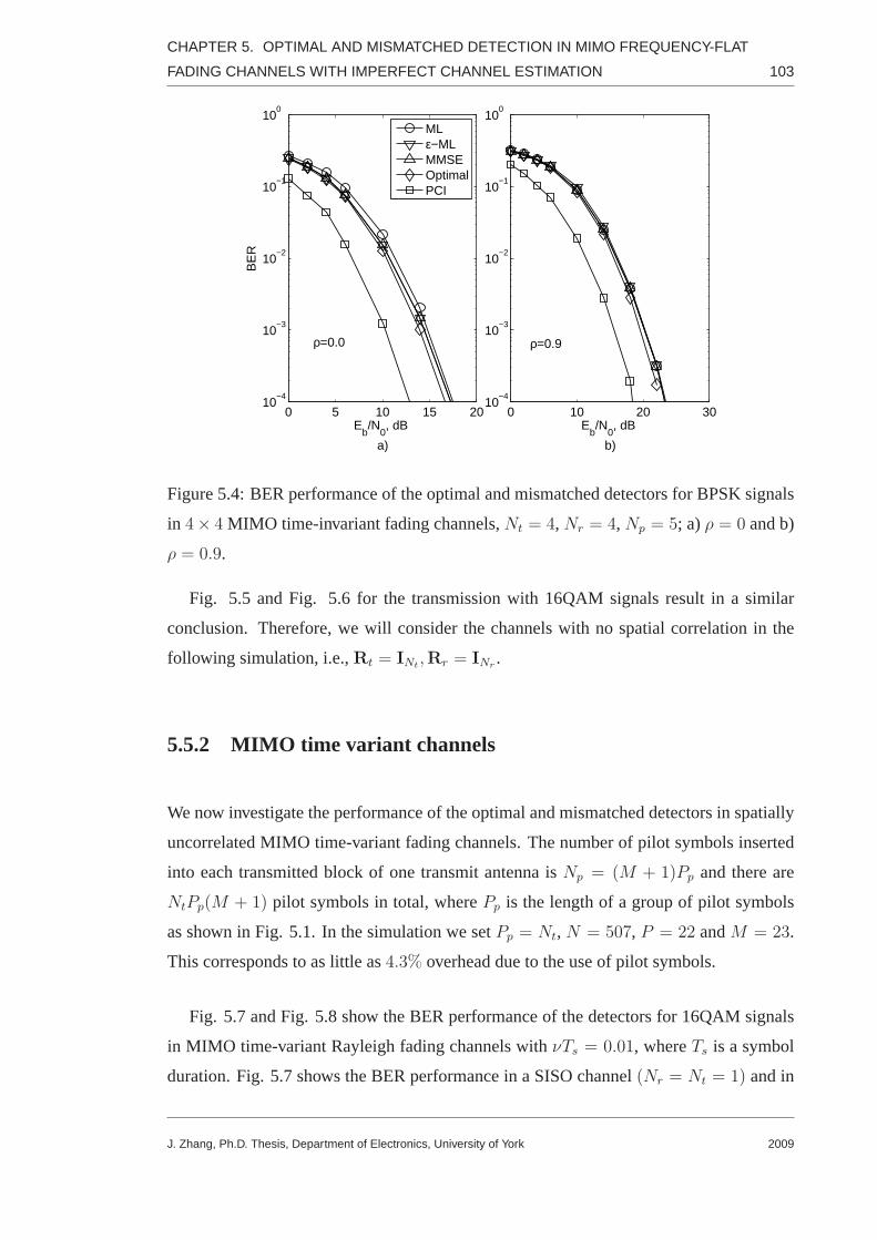
CHAPTER 5. OPTIMAL AND MISMATCHED DETECTION IN MIMO FREQUENCY-FLAT
FADING CHANNELS WITH IMPERFECT CHANNEL ESTIMATION 103
0 5 10 15 2010
−4
10−3
10−2
10−1
100
Eb/N
0, dB
a)
BE
R
MLε−MLMMSEOptimalPCI
0 10 20 3010
−4
10−3
10−2
10−1
100
Eb/N
0, dB
b)
ρ=0.0 ρ=0.9
Figure 5.4: BER performance of the optimal and mismatched detectors for BPSK signals
in 4× 4 MIMO time-invariant fading channels,Nt = 4,Nr = 4,Np = 5; a)ρ = 0 and b)
ρ = 0.9.
Fig. 5.5 and Fig. 5.6 for the transmission with 16QAM signalsresult in a similar
conclusion. Therefore, we will consider the channels with no spatial correlation in the
following simulation, i.e.,Rt = INt,Rr = INr
.
5.5.2 MIMO time variant channels
We now investigate the performance of the optimal and mismatched detectors in spatially
uncorrelated MIMO time-variant fading channels. The number of pilot symbols inserted
into each transmitted block of one transmit antenna isNp = (M + 1)Pp and there are
NtPp(M + 1) pilot symbols in total, wherePp is the length of a group of pilot symbols
as shown in Fig. 5.1. In the simulation we setPp = Nt, N = 507, P = 22 andM = 23.
This corresponds to as little as4.3% overhead due to the use of pilot symbols.
Fig. 5.7 and Fig. 5.8 show the BER performance of the detectorsfor 16QAM signals
in MIMO time-variant Rayleigh fading channels withνTs = 0.01, whereTs is a symbol
duration. Fig. 5.7 shows the BER performance in a SISO channel(Nr = Nt = 1) and in
J. Zhang, Ph.D. Thesis, Department of Electronics, University of York 2009

CHAPTER 5. OPTIMAL AND MISMATCHED DETECTION IN MIMO FREQUENCY-FLAT
FADING CHANNELS WITH IMPERFECT CHANNEL ESTIMATION 104
0 10 20 3010
−4
10−3
10−2
10−1
100
Eb/N
0, dB
a)
BE
R
MLε−MLMMSEOptimalPCI
0 10 20 3010
−4
10−3
10−2
10−1
100
Eb/N
0, dB
b)
ρ=0.0 ρ=0.9
Figure 5.5: BER performance of the optimal and mismatched detectors for 16QAM sig-
nals in2 × 2 MIMO time-invariant fading channels,Nt = 2, Nr = 2, Np = 3; a) ρ = 0
and b)ρ = 0.9.
0 5 10 15 2010
−4
10−3
10−2
10−1
100
Eb/N
0, dB
a)
BE
R
MLε−MLMMSEOptimalPCI
0 10 20 3010
−4
10−3
10−2
10−1
100
Eb/N
0, dB
b)
ρ=0.0 ρ=0.9
Figure 5.6: BER performance of the optimal and mismatched detectors for 16QAM sig-
nals in2 × 4 MIMO time-invariant fading channels,Nt = 2, Nr = 4, Np = 3; a) ρ = 0
and b)ρ = 0.9.
J. Zhang, Ph.D. Thesis, Department of Electronics, University of York 2009

CHAPTER 5. OPTIMAL AND MISMATCHED DETECTION IN MIMO FREQUENCY-FLAT
FADING CHANNELS WITH IMPERFECT CHANNEL ESTIMATION 105
0 5 10 15 20 25 3010
−6
10−5
10−4
10−3
10−2
10−1
100
Eb/N
0 (dB)
BE
R
ML 1×1ε−ML 1×1MMSE 1×1Optimal 1×1PCI 1×1ML 1×2ε−ML 1×2MMSE 1×2Optimal 1×2PCI 1×2
Figure 5.7: BER performance of the optimal and mismatched detectors for 16QAM sig-
nals in1× 1 and1× 2 channels;N = 507, P = 22, Pp = 1,M = 23.
a1×2 SIMO channel(Nt = 1, Nr = 2). We setPp = 1 andNp = 24 in both these cases.
In the SISO channel, at BER=10−2, the optimal detector outperforms the mismatched
detector with ML channel estimates by 6.1 dB and withǫ-ML channel estimates by 1.2
dB. However, the BER performance of the optimal detector and the mismatched detector
with MMSE channel estimates are similar. These detectors are inferior to the minimum
distance detector with perfect channel information (PCI) by2.4 dB. In the1 × 2 SIMO
channel, when BER=10−3, the improvement due to the use of the optimal detector in-
creases up to 10 dB compared with the mismatched detector with ML channel estimates
and up to 2.1 dB compared withǫ-ML channel estimates. The BER performance of the
optimal detector and that of the mismatched detector with MMSE channel estimates are
close; the difference in the performance is 0.2 dB. The gap between the BER curve of
the optimal detector and that of the minimum distance detector with PCI is 2 dB when
BER=10−2.
Fig. 5.8 shows simulation results for a2× 2 MIMO channel(Nt = Nr = 2); here, we
J. Zhang, Ph.D. Thesis, Department of Electronics, University of York 2009

CHAPTER 5. OPTIMAL AND MISMATCHED DETECTION IN MIMO FREQUENCY-FLAT
FADING CHANNELS WITH IMPERFECT CHANNEL ESTIMATION 106
−3 2 7 12 17 22 2710
−6
10−5
10−4
10−3
10−2
10−1
100
Eb/N
0 (dB)
BE
R
ML 2×2ε−ML 2×2MMSE 2×2Optimal 2×2PCI 2×2
Figure 5.8: BER performance of the optimal and mismatched detectors for 16QAM sig-
nals in a2× 2 channel ;N = 507, P = 22, Pp = 2,M = 23.
setPp = 2 andNp = 47. The optimal detector outperforms the mismatched detectorwith
ML channel estimates by 13 dB at BER=10−2; it outperforms the mismatched detector
with ǫ-ML channel estimates by 4.8 dB at BER=10−3; it also outperforms the mismatched
detector with MMSE channel estimates by 2.2 dB when BER=10−4. From this figure, we
find that the optimal detector provides better BER performance than mismatched detectors
which treat channel estimates as perfect for 16QAM signals,and the improvement in the
BER performance is increased when the number of antennas increases.
Fig. 5.9 and Fig. 5.10 show the BER performance of the optimal detector and mis-
matched detectors for BPSK signals. As shown in Fig. 5.9, in a SISO channel, when
BER=10−2, the optimal detector outperforms the mismatched detectorwith ML channel
estimates by 5.5 dB and the one withǫ-ML channel estimates by 0.5 dB. Similar to the
case of 16QAM signals in Fig. 5.7, the BER curves for the optimal detector and the mis-
matched detector with MMSE channel estimates are close. In a1×2 SIMO channel, when
BER=10−4, the benefit due to the use of the optimal detector is 7.4 dB compared with the
mismatched detector with ML channel estimates. Compared with the mismatched detec-
J. Zhang, Ph.D. Thesis, Department of Electronics, University of York 2009

CHAPTER 5. OPTIMAL AND MISMATCHED DETECTION IN MIMO FREQUENCY-FLAT
FADING CHANNELS WITH IMPERFECT CHANNEL ESTIMATION 107
0 5 10 15 20 25 3010
−6
10−5
10−4
10−3
10−2
10−1
100
Eb/N
0 (dB)
BE
R
ML 1×1ε−ML 1×1MMSE 1×1Optimal 1×1PCI 1×1ML 1×2ε−ML 1×2MMSE 1×2Optimal 1×2PCI 1×2
Figure 5.9: BER performance of the optimal and mismatched detectors for BPSK signals
in 1× 1 and1× 2 channels;N = 507, P = 22, Pp = 1,M = 23.
tor with ǫ-ML channel estimates, this benefit is 1.1 dB. It can be seen that the performance
of the optimal detector is similar with that of the mismatched detector with MMSE chan-
nel estimates, and it is inferior to the performance of the minimum distance detector with
PCI by 1.6 dB when BER= 10−4.
Fig. 5.10 shows simulation results in a2× 2 and2× 4 MIMO channels. In the2× 2
MIMO channel, the mismatched detector with ML estimates provides significantly worse
performance compared with others. The optimal detector provides significantly better per-
formance than the mismatched detector withǫ-ML channel estimates and it outperforms
the mismatched detector with MMSE channel estimates by 3 dB when BER=10−5. In
the2× 4 MIMO channels, the optimal detector significantly outperforms the mismatched
detectors withǫ-ML channel estimates. It also outperforms the mismatched detector with
MMSE channel estimates by 5.7 dB when BER=10−6.
J. Zhang, Ph.D. Thesis, Department of Electronics, University of York 2009
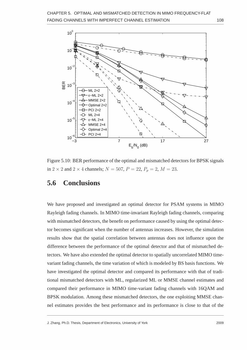
CHAPTER 5. OPTIMAL AND MISMATCHED DETECTION IN MIMO FREQUENCY-FLAT
FADING CHANNELS WITH IMPERFECT CHANNEL ESTIMATION 108
−3 7 17 2710
−6
10−5
10−4
10−3
10−2
10−1
100
Eb/N
0 (dB)
BE
R
ML 2×2ε−ML 2×2MMSE 2×2Optimal 2×2PCI 2×2ML 2×4ε−ML 2×4MMSE 2×4Optimal 2×4PCI 2×4
Figure 5.10: BER performance of the optimal and mismatched detectors for BPSK signals
in 2× 2 and2× 4 channels;N = 507, P = 22, Pp = 2,M = 23.
5.6 Conclusions
We have proposed and investigated an optimal detector for PSAM systems in MIMO
Rayleigh fading channels. In MIMO time-invariant Rayleigh fading channels, comparing
with mismatched detectors, the benefit on performance caused by using the optimal detec-
tor becomes significant when the number of antennas increases. However, the simulation
results show that the spatial correlation between antennasdoes not influence upon the
difference between the performance of the optimal detectorand that of mismatched de-
tectors. We have also extended the optimal detector to spatially uncorrelated MIMO time-
variant fading channels, the time variation of which is modeled by BS basis functions. We
have investigated the optimal detector and compared its performance with that of tradi-
tional mismatched detectors with ML, regularized ML or MMSEchannel estimates and
compared their performance in MIMO time-variant fading channels with 16QAM and
BPSK modulation. Among these mismatched detectors, the one exploiting MMSE chan-
nel estimates provides the best performance and its performance is close to that of the
J. Zhang, Ph.D. Thesis, Department of Electronics, University of York 2009

CHAPTER 5. OPTIMAL AND MISMATCHED DETECTION IN MIMO FREQUENCY-FLAT
FADING CHANNELS WITH IMPERFECT CHANNEL ESTIMATION 109
optimal detector in SISO time-variant fading channels whenQAM signals are transmit-
ted. However, the optimal detector significantly outperforms the mismatched detectors
in spatially uncorrelated MIMO time-variant fading channels when the number of anten-
nas increases. In this chapter, we have also shown that if theSIMO channel is spatially
uncorrelated, the optimal symbol-by-symbol detector of PSK signals is equivalent to the
mismatched detector with MMSE channel estimates. Note thatin the general case of
QAM symbols, the termY will depend ond and these two detectors are not equivalent.
J. Zhang, Ph.D. Thesis, Department of Electronics, University of York 2009

Chapter 6
Optimal Detection of OFDM Signals in
Frequency-Selective Fading Channels
with Imperfect Channel Estimation
Contents
6.1 Introduction . . . . . . . . . . . . . . . . . . . . . . . . . . . . . . . 110
6.2 Transmission model . . . . . . . . . . . . . . . . . . . . . . . . . . . 112
6.3 BEM of channel frequency response . . . . . . . . . . . . . . . . . . 114
6.4 Optimal and mismatched detectors . . . . . . . . . . . . . . . . . . 118
6.5 Iterative receiver . . . . . . . . . . . . . . . . . . . . . . . . . . . . . 123
6.6 Simulation Results . . . . . . . . . . . . . . . . . . . . . . . . . . . . 125
6.7 Conclusions . . . . . . . . . . . . . . . . . . . . . . . . . . . . . . . 131
6.1 Introduction
In previous chapters, we have investigated the optimal detector and compared it with
mismatched detectors in frequency-flat Rayleigh fading channels. The optimal detector
can also be used to detect OFDM signals in frequency-selective fading channels. In this
chapter, we derive and investigate the optimal detection ofOFDM signals.
J. Zhang, Ph.D. Thesis, Department of Electronics, University of York
110
2009

CHAPTER 6. OPTIMAL DETECTION OF OFDM SIGNALS IN FREQUENCY-SELECTIVE
FADING CHANNELS WITH IMPERFECT CHANNEL ESTIMATION 111
In OFDM systems, channel estimation is usually performed byemploying pilot
tones [17,21,24,127–138]. Then, the channel estimates aretreated as perfect in the tradi-
tional minimum distance detector. Motivated by the benefit caused by using the optimal
detector as shown in previous chapters, we derive an optimaldetector for OFDM signals
and specify it for spatially uncorrelated MIMO frequency-selective fading channels. We
compare the BER performance of this detector with that of mismatched detectors with
ML, regularized ML (ǫ-ML) or MMSE channel estimates for uncoded transmission. We
also investigate the performance of iterative receivers incorporating the optimal detector.
Specifically, four iterative receivers are considered: receivers with mismatched detectors
using ML, ǫ−ML or MMSE channel estimates, and a receiver with optimal detector at
the first iteration and the mismatched detector based on MMSEchannel estimates in sub-
sequent iterations.
In order to approximate the channel frequency response at data positions by using
channel estimates at positions of pilot symbols, many channel estimation schemes for
OFDM systems have been proposed in the literature [21, 70, 77, 129–131]. In [129], a
low rank approximation to the frequency domain linear MMSE channel estimator was
proposed by using singular value decomposition. In [130], the Wiener filter has been
investigated, and a robust MMSE channel estimator exploiting correlation in both time
and frequency domains was proposed in [131]. In this chapter, we also use channel
estimation based on BEMs, such as CE model [19, 21–24], GCE model[25], B-spline
functions [26–28], Slepian sequences [20, 29, 30] or KL basis functions [31, 32] to ap-
proximate correlated fading channels. After comparing theMSE performance of MMSE
channel estimators corresponding to these BEMs in Rayleigh frequency-selective fading
channels, we use the cubic B-splines to represent the channelfrequency response.
The rest of this chapter is structured as follows. In Section6.2, the transmission model
and communication scenarios are introduced. Different BEMsused to represent the chan-
nel frequency response are specified for frequency domain approximation in Section 6.3.
Section 6.4 describes the proposed optimal detector and mismatched detectors with dif-
ferent channel estimation schemes, and Section 6.5 describes the iterative receivers. Sim-
ulation results are given in Section 6.6, followed by conclusions in Section 6.7.
J. Zhang, Ph.D. Thesis, Department of Electronics, University of York 2009

CHAPTER 6. OPTIMAL DETECTION OF OFDM SIGNALS IN FREQUENCY-SELECTIVE
FADING CHANNELS WITH IMPERFECT CHANNEL ESTIMATION 112
6.2 Transmission model
We consider an MIMO OFDM system withN subcarriers,Nt transmit andNr receive
antennas. We assume that a data matrix ofN × Nt symbols is transmitted,Np × Nt of
which are pilot symbols and the othersNd ×Nt are data symbols, whereNd = N −Np.
The duration of an OFDM symbol without a cyclic prefix (CP) isTs = 1/∆f , where∆f
is the space between two neighboring subcarriers. In frequency domain, the pilot symbols
are inserted in groups ofPp symbols with the group period ofP symbols to construct an
OFDM symbol transmitted from one antenna as shown in Fig. 6.1. Here we follow the
the design of group pilot insertion in [24] and guaranteePp ≥ Nt. This OFDM symbol is
inverse Fourier transformed and a CP is added before the transmission.
Figure 6.1: Structure of an OFDM symbol transmitted from onetransmit antenna.
We consider transmission over MIMO time invariant frequency-selective fading chan-
nels withL path components, and assume that the inter-symbol interference (ISI) between
consecutive OFDM symbols is eliminated by using a CP of lengthLmaxT chosen to be
longer than the maximum channel delay, whereT = Ts/N . The channel from thekth
transmit antenna to therth receive antenna can be represented by the channel impulse
response
grk(τ) =L−1∑
l=0
αrk(l)δ(τ − τrk(l)), (6.1)
whereδ(τ) is the Dirac delta function,τrk(l) andαrk(l) are, respectively, the delay and
complex amplitude of thelth path in the channel. The channel frequency response at the
J. Zhang, Ph.D. Thesis, Department of Electronics, University of York 2009

CHAPTER 6. OPTIMAL DETECTION OF OFDM SIGNALS IN FREQUENCY-SELECTIVE
FADING CHANNELS WITH IMPERFECT CHANNEL ESTIMATION 113
ith subcarrier from thekth transmit antenna to therth receive antenna is given by
hrk(i) =L−1∑
l=0
αrk(l)e−j2πi∆fτrk(l). (6.2)
We denote anN×1 vectorhrk = [hrk(0), . . . , hrk(i), . . . , hrk(N−1)]T and anNtNrM×1
vector of the MIMO channel frequency responseh = [h1, . . . ,hr, . . . ,hNr]T , wherehr =
[h(0)r , . . . ,h
(i)r , . . . ,h
(N−1)r ] is a1×N row vector,h(i)
r = [hr1(i), . . . , hrk(i), . . . , hrNt(i)]
is a1×Nt row vector.
The path amplitudesαrk(l) are independent zero-mean complex Gaussian random
variables with exponential power delay profile given by [129]
ϑ(τ) = e−τ/τrms, (6.3)
whereτrms is the root-mean square width ofϑ(τ). The probability density function (PDF)
of a random delayτrk is uniform and given by
fτ (τ) =
1/(LmaxT ) if τ ∈ [0, LmaxT ],
0, otherwise.(6.4)
With these definitions, elements of the covariance matrixΥ0 = EhrkhHrk of the fading
in the frequency domain can be represented as [129]
[Υ0]m,n =1− e−LmaxT [(1/τrms)+j2π∆f(m−n)]
(1− e−LmaxT/τrms) (1 + j2π∆f(m− n)τrms), (6.5)
wheren andm denote two subcarriers of the OFDM symbol. Therefore, the dimension
of Υ0 isN ×N .
The spatial correlation matrix of transmit antennas is anNt×Nt symmetric matrixRt,
while the spatial correlation matrix of receive antennas isanNr × Nr symmetric matrix
Rr. We consider channels with no spatial correlation, i.e.,Rt = INt,Rr = INr
, where
IS is anS × S identity matrix. The joint spatial and frequency covariance matrix of the
MIMO channel is given by
Υ = E
hhH
= Rr ⊗Υ0 ⊗Rt. (6.6)
Note that the fading channel described above is only an example used in our simula-
tion. The results obtained below for the optimal detection can be applied to the case of an
arbitrary fading covariance matrixΥ0.
J. Zhang, Ph.D. Thesis, Department of Electronics, University of York 2009

CHAPTER 6. OPTIMAL DETECTION OF OFDM SIGNALS IN FREQUENCY-SELECTIVE
FADING CHANNELS WITH IMPERFECT CHANNEL ESTIMATION 114
At the receiver side, the CP is removed and the received signalis Fourier transformed.
In the frequency domain, the received OFDM symbol at therth receive antenna can be
written as:
zr(i) =Nt∑
k=1
hrk(i)sk(i) + nr(i), r = 1, · · · , Nr, (6.7)
wheresk(i) is a symbol transmitted at theith subcarrier from thekth transmit antenna
andnr(i) is the additive white Gaussian noise observed at therth receive antenna. We
denote anNNr × 1 vector of the received signal asz = [zT1 , . . . , zTr , . . . , z
TNr]T , where
zr = [zr(0), . . . , zr(N − 1)]T is anN × 1 vector; anNNr × 1 noise vector is given by
n = [nT1 , . . . ,nTr , . . . ,n
TNr]T , wherenr = [nr(0), . . . , nr(N−1)]T is anN×1 vector. We
consider scenarios where the noise samples at different receive antennas are uncorrelated
and assume that in the frequency domain, the noise covariance matrixRn0 = EnrnHr is the same for all receive antennas. TheN × N matrixRn0 characterizes correlation of
noise samples for a single receive antenna. Here we assume that the noise samples are
uncorrelated in frequency domain andRn0 = σ2nIN , whereσ2
n is the noise variance. Then
the total noise covariance matrix in frequency domain is given byRn = INr⊗Rn0.
6.3 BEM of channel frequency response
A channel frequency responseh(f) can be represented by a BEM as
h(f) ≈ h(f) =M∑
m=1
amB(f,m), (6.8)
whereB(f,m) are basis functions,am are expansion coefficients, andM is the number
of basis functions. The BEM allows transforming the nonparametric estimation problem
to a parametric one: we need to estimateM unknown expansion coefficients instead of
estimatingh(f) as a function off . The difference betweenh(f) and h(f) represents a
modeling error, which can be made negligible by choosingM large enough [20,27]; then,
we can assume thath(f) = h(f). However, depending on an estimation technique, a large
M may also result in a high noise error (as opposed to the modeling error) [26]. Moreover,
a largeM will lead to high complexity of the receiver. Therefore, it is important to choose
an appropriateM to guarantee that the receiver provides a high estimation performance
and requires a low computational load.
J. Zhang, Ph.D. Thesis, Department of Electronics, University of York 2009

CHAPTER 6. OPTIMAL DETECTION OF OFDM SIGNALS IN FREQUENCY-SELECTIVE
FADING CHANNELS WITH IMPERFECT CHANNEL ESTIMATION 115
We denoteB as anN×M matrixB containing samples of basis functions at subcarrier
frequencies. The channel frequency response between thekth transmit antenna and the
rth receive antenna is then modeled as
hrk = Ba(rk), (6.9)
where theM × 1 vectora(rk) = [a(rk)1 , . . . , a
(rk)M ]T represents the BEM coefficients be-
tween thekth transmit antenna and therth receive antenna, and these coefficients are
constant over an OFDM symbol. The matrixB can be split into two parts as follows. The
Np ×M matrixBp contains samples of basis functions at subcarriers occupied by pilot
symbols:[Bp]i,m = [B]ξi,m. TheNd ×M matrixBd contains samples of basis functions
at subcarriers occupied by data symbols:[Bd]i,m = [B]fi,m. With these notations, the
received signal can be represented as
z = Ψa+ n, (6.10)
where
a =
a(1)
...
a(r)
...
a(Nr)
, a(r) =
a(r1)
...
a(rk)
...
a(rNt)
,
andΨ = INr⊗ΨNt
is anNNr ×MNtNr matrix,ΨNt= [Ψ(1), . . . ,Ψ(k), . . . ,Ψ(Nt)] is
anN ×MNt matrix,Ψ(k) = SkB where theN ×N matrixSk is given by
Sk = diag[sk(0), . . . , sk(i), . . . , sk(N − 1)]. (6.11)
The received signal corresponding to subcarriers occupiedby data and pilot symbols
are modeled, respectively, as
zd = Ψda+ nd, zp = Ψpa+ np. (6.12)
According to (6.12), theNNr × 1 vectorz is split into a vector of received data symbols:
zd = [vT1 , . . . ,vTr , . . . ,v
TNr]T is anNdNr×1 vector, where[vr]i = zr(fi), and anNpNr×1
vector of received pilot symbolszp = [uT1 , . . . ,uTr , . . . ,u
TNr]T , where[ur]i = zr(ξi). Sim-
ilarly, the noise vectorn is split into anNdNr × 1 vectornd = [xT1 , · · · ,xTr , · · · ,xTNr]T ,
where[xTr ]i = nr(fi) and anNpNr × 1 vectornp = [wT1 , · · · ,wT
r , · · · ,wTNr]T , where
J. Zhang, Ph.D. Thesis, Department of Electronics, University of York 2009

CHAPTER 6. OPTIMAL DETECTION OF OFDM SIGNALS IN FREQUENCY-SELECTIVE
FADING CHANNELS WITH IMPERFECT CHANNEL ESTIMATION 116
[wTr ]i = nr(ξi). Correspondingly, the matrixΨ is split into a matrix of transmitted data
symbolsΨd = INr⊗ΨNt
d , where
ΨNt
d = [Ψ(1)d , . . . ,Ψ
(k)d , . . . ,Ψ
(Nt)d ], Ψ
(k)d = S
(k)d Bd,
S(k)d = diag[sk(0), . . . , sk(fi), . . . , sk(Nd − 1)],
and a matrix of transmitted pilot symbolsΨp = INr⊗ΨNt
p , where
ΨNtp = [Ψ
(1)p , . . . ,Ψ
(k)p , . . . ,Ψ
(Nt)p ], Ψ
(k)p = S
(k)p Bp,
S(k)p = diag[sk(0), . . . , sk(ξi), . . . , sk(Np − 1)].
For different BEMs, the calculation of the matrixB and the vectora are different. In
this chapter, we consider the following BEMs: CE BEM, GCE BEM, cubic B-splines,
Slepian sequences and KL basis functions.
6.3.1 CE basis functions
The CE BEM is widely used [19, 21–23], but it can result in large modeling errors. For
the CE model, elements of the matrixB are given by [21]
[B]n,m = ej2π∆fn(m−M2), m = 1, . . . ,M, n = 1, . . . , N. (6.13)
6.3.2 GCE basis functions
An improved modeling performance is obtained by using the GCEBEM applying a set
of complex exponentials with the period longer than the window length related to the CE
BEM [25,70]. For the GCE model, elements of the matrixB are given by [25,70]
[B]n,m = ej2π∆f
κn(m−M
2), m = 1, . . . ,M, n = 1, . . . , N, (6.14)
whereκ is a real number which is larger than1; usually,κ = 2 is used [25].
Note that there is another ways to build the generalized complex exponential functions,
i.e.,
[B]n,m = e−j2π∆f(n−1)(m−1)LmaxTM−1 , m = 1, . . . ,M, n = 1, . . . , N. (6.15)
J. Zhang, Ph.D. Thesis, Department of Electronics, University of York 2009

CHAPTER 6. OPTIMAL DETECTION OF OFDM SIGNALS IN FREQUENCY-SELECTIVE
FADING CHANNELS WITH IMPERFECT CHANNEL ESTIMATION 117
By using (6.15), we assume that the considered channel (6.7) is equivalent to a multipath
channel
grk(τ) =M−1∑
m=0
αrk(m)δ(
τ − m
MLmaxT
)
, (6.16)
and the task of the estimator becomes to estimateM correspondingαrk. It indicates that
the number of basis functions does not depend onN anymore. In this chapter, we just
consider the GCE defined in (6.14), and the details of the performance of the modified
GCE as (6.15) can be found in our previous publications [41].
6.3.3 Cubic B-splines functions
Cubic B-splines have previously been used for estimating the channel frequency response
in the underwater acoustic channel [139]. To build basis functions, we use the cubic
B-splines [76]
ϕ(f) =
23− f2
F 2 +|f |3
2F 3 , if |f | < F,
16(2− |f |
F)3, if F ≤ |f | < 2F ,
0, otherwise,
(6.17)
whereF = (N − 1)∆f/(M − 3) and the basis functions are given byϕm(f) = ϕ[f −(m− 2)∆f ], wherem = 1, . . . ,M . Elements of the matrixB are given by
[B]n,m = ϕm(n− 1), m = 1, . . . ,M, n = 1, . . . , N. (6.18)
6.3.4 Slepian sequences
Slepian sequences are a set of orthogonal functions which are widely used for channel
estimation both in time and frequency domains [20, 30, 67]. Let considerM Slepian se-
quencesum(n) with lengthN bandlimited to the frequency range[−12τmax∆f,
12τmax∆f ].
Such sequences are the eigenvectors of the following equation
N∑
q=1
sin(πτmax∆f(q − n))
π(q − n)um(q) = λmum(n), (6.19)
whereλm is an eigenvalue indicating the fraction of energy contained in the frequency
range[−12τmax∆f,
12τmax∆f ] of the corresponding eigenvector [67]. The eigenvalues are
J. Zhang, Ph.D. Thesis, Department of Electronics, University of York 2009

CHAPTER 6. OPTIMAL DETECTION OF OFDM SIGNALS IN FREQUENCY-SELECTIVE
FADING CHANNELS WITH IMPERFECT CHANNEL ESTIMATION 118
ordered starting with the maximum one:λ1 ≥ λ2 ≥ . . . ≥ λN ≥ 0. Therefore,um(n) is
themth most concentrated Slepian sequence. According to [29], Mshould be chosen to
provideλm close to 1 whenm ≤ M and close to 0 whenm ≥ M . We intend to use the
Slepian sequences over the frequency range[0, τmax∆f ]. Then, the basis functions can be
represented as
[B]n,m = um(n)e−jπnτmax∆f , m = 1, . . . ,M, n = 1, . . . , N. (6.20)
6.3.5 KL BEM
The KL BEM is optimal in terms of the mean square error (MSE) [31, 32], which is a
reduced-rank decomposition of channels whose statisticalinformation is known at the
receiver side. The KL basis functionsvm(n) are eigenvectors of the fading covariance
matrix. Specifically, the covariance matrix of the fading inthe frequency domain isΥ0
which is obtained in (6.5). We also order the eigenvaluesλm of Υ0 as:λ1 ≥ λ2 ≥ . . . ≥λN ≥ 0, and assume that whenm is larger than a fixed valueM << N , λm decreases
rapidly and can be neglected [32]. Then, the KL basis functions can be represented as
[B]n,m = vm(n), m = 1, . . . ,M, n = 1, . . . , N. (6.21)
6.4 Optimal and mismatched detectors
6.4.1 Optimal detection
We now derive an optimal detector by maximizing the PDFp(zd|Sd, zp) of the received
signalzd and the received pilot signalzp, conditioned on the transmitted data symbolsSd:
Sd,opt = arg maxSd∈A
NdNt
p(zd|Sd, zp)
= arg maxSd∈A
NdNt
λopt(Sd) , (6.22)
where the metricλopt(Sd) is given by
λopt(Sd) = ln [p(zd|Sd, zp)] , (6.23)
J. Zhang, Ph.D. Thesis, Department of Electronics, University of York 2009

CHAPTER 6. OPTIMAL DETECTION OF OFDM SIGNALS IN FREQUENCY-SELECTIVE
FADING CHANNELS WITH IMPERFECT CHANNEL ESTIMATION 119
and the alphabetA includes symbols corresponding to all constellation points. The PDF
p(zd|Sd, zp) can be obtained from the PDFp(zd|Sd, a) of the received signal vectorzd
conditioned on the transmitted dataSd and channel parameters (expansion coefficients)a
by integrating out the channel parametersa which are treated asnuisance parameters:
p(zd|Sd, zp) =∫
p(zd|Sd, a)f(a|zp)da, (6.24)
wherep(zd|Sd, a) is given by
p(zd|Sd, a) =1
πNdσ2n
exp
−‖zd −Ψda‖2σ2n
. (6.25)
The posterior PDF f(a|zp) of the expansion coefficientsa subject to the received pi-
lot signalszp is Gaussian with the mean vector(ΨHp Ψp + σ2
nR−1a )
−1ΨHp zp and covari-
ance matrix(ΨHp Ψp + σ2
nR−1a ) [113], where the covariance matrixRa is given by
Ra = EaaH = Rr ⊗ Rt ⊗ Λ0, andM ×M matrix Λ0 = E
(a(rk))Ha(rk)
is the
covariance matrix of the expansion coefficientsa(rk) for the frequency response between
thekth transmit antenna and therth receive antenna. The matrixΛ0 can be obtained from
the fading covariance matrixΥ0 by requiring that
EhrkhHrk = EhrkhHrk = Υ0. (6.26)
This requirement means that the correlation matrixΛ0 results in fading correlationΥ0 in
the frequency domain. By substituting (6.9) in (6.26), we obtain
BΛ0BH = Υ0. (6.27)
Multiplying both sides of (6.27) byΩ = (BHB)−1BH from the left and byΩH from the
right, we arrive at
Λ0 = ΩΥ0ΩH . (6.28)
The optimal detector finds a data matrixSd that maximizes the metric (6.23) which
is obtained by substituting the Gaussian PDFf(a|zp) in (6.24) and then the result of
integration - in (6.23). After some algebra, we arrive at
Sd,opt = arg maxSd∈A
NdNt
ln
[∫
p(zd|Sd, a)f(a|zp)da]
= arg maxSd∈A
NdNt
ln
[∫
eσ−2n [2ℜ(aHΨH
dzd)−aHΨH
dΨda]f(a|zp)da
]
= arg maxSd∈A
NdNt
σ−2n
(
ΨHd zd +ΨH
p zp)H (
ΨHd Ψd +ΨH
p Ψp + σ2nR
−1a
)−1
×(
ΨHd zd +ΨH
p zp)
− ln∣
∣ΨHd Ψd +ΨH
p Ψp + σ2nR
−1a
∣
∣
, (6.29)
J. Zhang, Ph.D. Thesis, Department of Electronics, University of York 2009
CHAPTER 6. OPTIMAL DETECTION OF OFDM SIGNALS IN FREQUENCY-SELECTIVE
FADING CHANNELS WITH IMPERFECT CHANNEL ESTIMATION 120
However, it is unfeasible to solve this optimization problem for a highNd due to ex-
tremely high computational complexity. If QAM symbols with2K constellation points
are transmitted, we have to calculate the metric2KNdNt times. In order to reduce the
computational load, we separate the data into groups of symbols, each containingG data
symbols. We repeat the detectionNd/G times to recover all the symbols. In this case, the
optimal metric should be calculatedNd
G2KNtG times, which can be significantly smaller
compared with2KNdNt .
As the simplest case, we considerG = 1, which indicates that the optimal symbol-
by-symbol detection scheme is applied, and we only detectNt data symbols at once. In
this case, the expressions above are simplified:zd = [z1(fi), . . . , zr(fi), . . . , zNr(fi)]
T ,
Ψ(k)d = sk(fi)Bd, andBd becomes a1 × M vector corresponding to samples of ba-
sis functions at theith subcarrier frequency. Although the computational load is re-
duced, the detection performance will be degraded. Therefore, we also consider the
optimal detection with1 < G ≪ Nd to trade off the complexity and detection perfor-
mance. In this case, expressions above are modified:zd = [vT1 , . . . ,vTr , . . . ,v
TNr]T and
vr = [zr(fi), . . . , zr(fi+G−1)]T ; Bd becomes anG×M matrix corresponding to samples
of basis functions at thefi-th to (fi + G − 1)-th subcarriers. Investigating the improve-
ment of BER performance due to using the optimal detector compared with traditional
mismatched detectors is the main target of this chapter, andmethods to analyze the com-
plexity and reduce the computational load of this optimal detector will be discussed in
further works.
6.4.2 Mismatched detection
Now, we consider mismatched detectors applying three different channel estimators: ML,
ǫ-ML or MMSE estimators. The ML channel estimate is given by
aML = (ΨHp Ψp)
−1ΨHp zp. (6.30)
The performance of the ML channel estimator is significantlydegraded in noisy scenarios.
A better performance is obtained when using regularized ML channel estimation based
on the diagonal loading:
aǫ = (ΨHp Ψp + ǫσ2
nIMNtNr)−1ΨHp zp, (6.31)
J. Zhang, Ph.D. Thesis, Department of Electronics, University of York 2009

CHAPTER 6. OPTIMAL DETECTION OF OFDM SIGNALS IN FREQUENCY-SELECTIVE
FADING CHANNELS WITH IMPERFECT CHANNEL ESTIMATION 121
whereǫ is a positive regularization parameter and in our simulation we useǫ = 1. We
also consider the MMSE channel estimation that takes the statistical information of the
channel fading into account,
aMMSE = (ΨHp Ψp + σ2
nR−1a )
−1ΨHp zp. (6.32)
A mismatched detector uses the minimum distance detector that treats the channel
estimates as perfect channel information and decides on thetransmitted data symbols by
minimizing the Euclidean distance
Sd,mis = arg minSd∈ANt
λmis(Sd) ,
= arg minSd∈ANt
‖zd −Ψda‖2σ2n
, (6.33)
wherea = aML for ML channel estimates (6.30), ora = aǫ for ǫ-ML channel estimates
(6.31) ora = aMMSE for MMSE channel estimates (6.32).
6.4.3 Complexity analysis
Now, we analyze the complexity of the optimal detector with symbol-by-symbol detection
scheme (G = 1) for SISO systems. In this case, quantities in (6.29) are significantly
simplified: Sd = d, whered is a data symbol;zd = z1(fi); Ψd = dBd, whereBd
becomes a1×M vector. Accordingly, we can simplify (6.29) as
dopt = argmaxd∈A
σ−2n
(
d∗zdBHd +ΨH
p zp)H (|d|2BH
d Bd +ΨHp Ψp + σ2
nR−1a
)−1
×(
d∗zdBHd +ΨH
p zp)
− ln∣
∣|d|2BHd Bd +ΨH
p Ψp + σ2nR
−1a
∣
∣
= argmaxd∈A
σ−2n |d|2|zd|2BdYBH
d + 2σ−2n ℜdz∗dBdYΨpzp
+ σ−2n zHp ΨpYΨH
p zp + ln |Y|
, (6.34)
whereY =(
|d|2BHd Bd +ΨH
p Ψp + σ2nR
−1a
)−1is anM × M matrix and(·)∗ denotes
complex conjugate. If we assume that (i) the same pilot symbols are inserted into every
OFDM symbol (Ψp is the same for all OFDM symbols); (ii) the covariance matrixof
fadingRa andσ2n are constant overNc OFDM symbols and known at the receiver side,
the matrixY will depend only on the possible magnitudes of data symbols|d|, pilot
J. Zhang, Ph.D. Thesis, Department of Electronics, University of York 2009
CHAPTER 6. OPTIMAL DETECTION OF OFDM SIGNALS IN FREQUENCY-SELECTIVE
FADING CHANNELS WITH IMPERFECT CHANNEL ESTIMATION 122
symbols and BEM samplesBd andBp. The pilot symbols and all possible values of
|d|2 (we denote this number asD) are known to the receiver. Moreover,Bd andBp are
also available, since positions of data and pilot symbols are fixed. Therefore, we can
precompute scalarsln |Y| for all possible|d|. This precomputation requiresO(M3NdD)
complex multiplications. E.g., for 16QAM modulation, the number of possible|d| is
D = 4; thus the number of scalarsln |Y| is 4Nd. The scalarBdYBHd in the first term of
(6.34),1×Np vectorBdYΨp in the second term of (6.34) andNp ×Np matrixΨpYΨHp
in the third term of (6.34) can also be precomputed for allD possible|d|. In total, there
are (N2p + Np + Nd)D complex numbers to be kept in memory. To precompute these
numbers requiresO(M3NdD) complex multiplications. These complex numbers can be
used for detecting allNc OFDM symbols. Therefore, the average number of complex
multiplications for all the precomputation isO(
M3D+NpM2+N2pM
Nc
)
per one data symbol.
We now denote:ρ = BdYBHd , w = BdYΨp, andΞ = ΨpYΨH
p . Then, the equation
(6.34) is transformed to
dopt = argmaxd∈A
σ−2n |d|2|zd|2ρ+ 2σ−2
n ℜdz∗dwzp+ σ−2n zHp Ξzp + ln |Y|
.(6.35)
For each OFDM symbol, in (6.35), the scalarswzp andzpΞzp can be computed once and
reused for detecting all data symbols. Thus, only|d|2|zd|2 in the first term anddz∗d in the
second term require to be computed symbol-by-symbol. Therefore, with the precomputa-
tion as explained above, the average number of complex multiplications required to detect
one data symbol isN2
p+2Np+4
Nd+ 2K +D.
Now, we analyze the complexity of a mismatched detector treating the MMSE chan-
nel estimates as perfect. For a fixedσ2n, we can precompute theM × Np matrix
(ΨHp Ψp + σ2
nR−1a )
−1ΨHp in (6.32) and keep it in memory; the number of complex mul-
tiplications required for this precomputation isO(M3 + NpM2). This matrix can also
be calculated once and reused to detect allNc OFDM symbols as well, for channels with
fixed Ra andσ2n. Therefore, the number of complex multiplications for thisprecompu-
tation isO(
M3+NpM2
NcNd
)
per one data symbol. The number of complex multiplications
required by a minimum distance detector (6.33) isM2K . Table. 1 shows the complexity
of the optimal and mismatched detectors.
It is seen that whenNc is large, which indicates that the channel statistics change
slowly (Ra andσ2n keep constant for numerous OFDM symbols), to detect one datasym-
J. Zhang, Ph.D. Thesis, Department of Electronics, University of York 2009
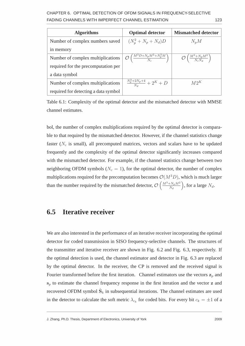
CHAPTER 6. OPTIMAL DETECTION OF OFDM SIGNALS IN FREQUENCY-SELECTIVE
FADING CHANNELS WITH IMPERFECT CHANNEL ESTIMATION 123
Algorithms Optimal detector Mismatched detector
Number of complex numbers saved
in memory
(N2p +Np +Nd)D NpM
Number of complex multiplications
required for the precomputation per
a data symbol
O(
M3D+NpM2+N2pM
Nc
)
O(
M3+NpM2
NcNd
)
Number of complex multiplications
required for detecting a data symbol
N2p+2Np+4
Nd+ 2K +D M2K
Table 6.1: Complexity of the optimal detector and the mismatched detector with MMSE
channel estimates.
bol, the number of complex multiplications required by the optimal detector is compara-
ble to that required by the mismatched detector. However, ifthe channel statistics change
faster (Nc is small), all precomputed matrices, vectors and scalars have to be updated
frequently and the complexity of the optimal detector significantly increases compared
with the mismatched detector. For example, if the channel statistics change between two
neighboring OFDM symbols (Nc = 1), for the optimal detector, the number of complex
multiplications required for the precomputation becomesO(M3D), which is much larger
than the number required by the mismatched detector,O(
M3+NpM2
Nd
)
, for a largeNd.
6.5 Iterative receiver
We are also interested in the performance of an iterative receiver incorporating the optimal
detector for coded transmission in SISO frequency-selective channels. The structures of
the transmitter and iterative receiver are shown in Fig. 6.2and Fig. 6.3, respectively. If
the optimal detection is used, the channel estimator and detector in Fig. 6.3 are replaced
by the optimal detector. In the receiver, the CP is removed andthe received signal is
Fourier transformed before the first iteration. Channel estimators use the vectorszp and
sp to estimate the channel frequency response in the first iteration and the vectorz and
recovered OFDM symbolSk in subsequential iterations. The channel estimates are used
in the detector to calculate the soft metricλck for coded bits. For every bitck = ±1 of a
J. Zhang, Ph.D. Thesis, Department of Electronics, University of York 2009

CHAPTER 6. OPTIMAL DETECTION OF OFDM SIGNALS IN FREQUENCY-SELECTIVE
FADING CHANNELS WITH IMPERFECT CHANNEL ESTIMATION 124
Figure 6.2: Block-diagram of the transmitter with turbo encoder and channel interleaver
for SISO channels.
Figure 6.3: Block-diagram of the iterative receiver for SISOchannels.
received symbol,k = 1, . . . , K, thea posteriorilog-likelihood ratio (LLR) is computed
as
λck = ln
[∑
d∈A+
ke−λ(d)
∏
i 6=k P (ci)∑
d∈A−
ke−λ(d)
∏
i 6=k P (ci)
]
, (6.36)
where thea priori probabilityP (ci) of a symbol bit is expressed in terms of itsa priori
LLR L(ci) [118]:
P (ci) =1
2
[
1 + ci tanh
(
1
2L(ci)
)]
,
A±k = d ∈ A|ck = ±1, and the metricλ(d) depends on the detector used. For the first
iteration, we have
λck = ln∑
d∈A+
k
e−λ(d) − ln∑
d∈A−
k
e−λ(d). (6.37)
After being de-interleaved, LLRsλck are decoded by a soft-input soft-output turbo
decoder. The hard decisions of the LLRs of decoded bits are interleaved and mapped
to the QAM constellation to rebuild the data symbols. The pilot symbols are inserted
to recover the OFDM symbol in the frequency domain. The recovered OFDM symbol
is feedback to the channel estimator or to the optimal detector. The channel estimates,
J. Zhang, Ph.D. Thesis, Department of Electronics, University of York 2009

CHAPTER 6. OPTIMAL DETECTION OF OFDM SIGNALS IN FREQUENCY-SELECTIVE
FADING CHANNELS WITH IMPERFECT CHANNEL ESTIMATION 125
LLRs of coded bits and LLRs of decoded bits are refined once per iteration by treating
all recovered data symbols as pilot symbols. Since the channel estimator and detector
applied at the first iteration and those applied in the following iterations can be different,
the schemes used at the receiver are correspondingly modified. Depending on the detector
used and whether it is the first or a subsequent iteration, four different iterative receivers
are considered:
1. ML-ML receiver: The ML channel estimator is used in all iterations. At the first
iteration, the ML estimator (6.30) is used to estimate the channel frequency response
based on transmitted pilot symbols. In the following (three) iterations, the number of input
pilot symbols used to obtain the frequency response estimateshML = BaML is extended
from Np to N , all recovered symbols are used as pilot symbols to refine thechannel
estimation and signal detection, and consequently,Ψp, Bp, zp in (6.30) are replaced by
Ψ, B andz, respectively.
2. ǫ-ML-ǫ-ML receiver: This receiver is similar to theML-ML receiver with replace-
mentaML by aǫ according to (6.31).
3. MMSE-MMSE receiver: The receiver is similar to theML-ML receiver with re-
placementaML by aMMSE according to (6.32).
4. Optimal-MMSEreceiver: The optimal detector is used at the first iteration; MMSE
channel estimation and minimum distance detector are used in the following three itera-
tions.
6.6 Simulation Results
In this section, numerical results obtained by simulation are presented. We consider
frequency-selective fading channels withL = 6 paths, and setLmax = 10, Pp = Nt,
N = 461, P = 20 andM = 23. Firstly, we compare the performance of the MMSE
channel estimators corresponding to different BEMs for SISOmultipath channels with
differentτrms. Then, the performance of the optimal detector with group symbol detection
(G > 1) in SISO channels is also considered. As the improvement of the BER perfor-
J. Zhang, Ph.D. Thesis, Department of Electronics, University of York 2009

CHAPTER 6. OPTIMAL DETECTION OF OFDM SIGNALS IN FREQUENCY-SELECTIVE
FADING CHANNELS WITH IMPERFECT CHANNEL ESTIMATION 126
mance is not significant even ifG = 7, in the following simulation scenarios, we only
considerG = 1. We then compare the BER performance of four iterative receivers for
turbo coded transmission in SISO multipath channels. Finally, we consider the trans-
mission with 16QAM and BPSK modulation in MIMO channels and concentrate on the
comparison between the BER performance of the optimal detector and that of the mis-
matched detector with MMSE channel estimates for uncoded transmission. The average
SNR is given by
ζ =NtEsσ
2h
σ2n
, (6.38)
whereEs is the average energy of data symbols andσ2h is the variance of channel fre-
quency response between a pair of transmit and receive antennas. The average bit energy
to noise ratio is defined asEb/N0 = ζ/(NtK). Simulation results below represent the
MSE or BER versusEb/N0.
Firstly, we compare the MSE performance of the mismatched detector with MMSE
channel estimates based on different BEMs. The MSE in one simulation trial is calculated
as
MSE=
∑Nr
r=1
∑Nt
k=1
∑N−1i=0 |hr,k(i)− hr,k(i)|2
∑Nr
r=1
∑Nt
k=1
∑N−1i=0 |hr,k(i)|2
. (6.39)
Then these MSEs are averaged over all simulation trials. Fig. 6.4 shows the MSE perfor-
mance of the MMSE channel estimators in SISO channels withτrms = 5T . The CE BEM
shows a poor performance compared to the other BEMs, while theKL BEM provides the
best MSE performance. The other BEMs show the performance similar to that of the KL
BEM. We have also considered a channel withτrms = T ; the simulation results show a
similar performance. However, both the Slepian and KL BEMs require the knowledge of
statistical characteristics of the fading, which is not practical for ML andǫ-ML channel
estimation. The cubic B-splines provide performance close to that of the KL BEM in most
scenarios. However, as B-splines have a finite support that issignificantly smaller thanN ,
as seen from (6.17) and (6.18), the complexity of estimatorsusing B-splines can be sig-
nificantly lower than that of the other BEMs. Moreover, the complexity of the minimum
distance detector applying B-splines channel estimates is lower than that of the minimum
distance detector applying other BEMs channel estimates. Based on (6.33), in order to
detect allNd data symbols, the number of complex multiplications required by the mini-
mum distance detector applying other BEMs channel estimatesisO(MNd2K), while the
number of required complex multiplications for cubic B-splines is onlyO(4Nd2K), as
J. Zhang, Ph.D. Thesis, Department of Electronics, University of York 2009

CHAPTER 6. OPTIMAL DETECTION OF OFDM SIGNALS IN FREQUENCY-SELECTIVE
FADING CHANNELS WITH IMPERFECT CHANNEL ESTIMATION 127
0 5 10 15 20 25 30−35
−30
−25
−20
−15
−10
−5
0
Eb/N
0 (dB)
MS
E (
dB)
CEGCECubicSlepianKL
Figure 6.4: MSE performance of MMSE channel estimators withdifferent BEMs for
BPSK signals in SISO channels,L = 6, Lmax = 10,N = 461, P = 20, Pp = 1,M = 23,
τrms = 5T .
seen from (6.17). For these reasons, we use B-splines as basisfunctions in the following
simulations.
Simulation results for transmission of BPSK signals in SISO channels with different
G are shown in Fig. 6.5. For BER= 10−3, the optimal detector withG = 1 is inferior to
the minimum distance detector with perfect channel information by 1.7 dB. ForG = 3,
this is reduced to 1.4 dB, and forG = 7 it is reduced to 1 dB. Thus, the performance
of the optimal detector is slightly improved if the number ofsymbols in detection groups
increases. However, compared with the symbol-by-symbol detection (G = 1), the com-
plexity is also significantly increased. In the following simulation, we will only consider
the caseG = 1.
We investigate the performance of the optimal and mismatched detectors for coded
transmission of 16QAM symbols(K = 4) in SISO channels. The iterative receivers and
J. Zhang, Ph.D. Thesis, Department of Electronics, University of York 2009

CHAPTER 6. OPTIMAL DETECTION OF OFDM SIGNALS IN FREQUENCY-SELECTIVE
FADING CHANNELS WITH IMPERFECT CHANNEL ESTIMATION 128
20 22 24 26 28 3010
−4
10−3
10−2
Eb/N
0 (dB)
BE
R
Optimal G=1Optimal G=3Optimal G=7PCI
Figure 6.5: BER performance of the optimal detector againstG for the transmission of
BPSK signals in SISO channels;L = 6, Lmax = 10, τrms = 5T , N = 461, P = 20,
Pp = 1,M = 23.
rate-13
turbo code with generating polynomial[013, 015] are used to improve the BER and
MSE performance. Fig. 6.6 shows the BER performance of the iterative receivers after
4 iterations. The receiver using the optimal detection at the first iteration significantly
outperforms receivers using mismatched detectors with ML and ǫ-ML channel estimates.
At BER = 10−3, the improvement in the detection performance is6.3 dB against the
ML-ML receiver and2.0 dB against theǫ-ML-ǫ-ML receiver. Both theMMSE-MMSE
receiver and theOptimal-MMSEreceiver provide the BER performance close to the case
of perfect channel information; the gap between the BER curves of theOptimal-MMSE
receiver and that of theMMSE-MMSEreceiver is approximately 0.6 dB at BER=10−3.
We now compare the performance of the optimal detector for uncoded symbols with
that of mismatched detectors in MIMO channels. Fig. 6.7 shows the BER performance of
the detectors for 16QAM signals in MIMO channels. Fig. 6.7(a) shows the BER perfor-
mance in SISO channels(Nr = Nt = 1) and in1× 2 SIMO channels(Nt = 1, Nr = 2).
J. Zhang, Ph.D. Thesis, Department of Electronics, University of York 2009

CHAPTER 6. OPTIMAL DETECTION OF OFDM SIGNALS IN FREQUENCY-SELECTIVE
FADING CHANNELS WITH IMPERFECT CHANNEL ESTIMATION 129
0 2 4 6 8 10 12 14 16 1810
−6
10−5
10−4
10−3
10−2
10−1
100
Eb/N
0 (dB)
BE
R
ML−MLε−ML−ε−MLMMSE−MMSEOptimal−MMSEPCI
Figure 6.6: BER performance of iterative receivers applyingoptimal and/or mismatched
detection for 16QAM signals in SISO channels, rate 1/3 turbocode, 4 iterations;L = 6,
Lmax = 10, τrms = 5T ,N = 461, P = 20, Pp = 1,M = 23.
We setPp = 1 andNp = 24 in both these cases. In1 × 1 SISO channels, at BER=10−2,
the optimal detector outperforms the mismatched detector with ML channel estimates by
13 dB and withǫ-ML channel estimates by 1.2 dB. However, the BER performance of the
optimal detector and the mismatched detector with MMSE channel estimates are similar.
These detectors are inferior to the minimum distance detector with perfect channel infor-
mation (PCI) by 2 dB. In1×2 SIMO channels, the mismatched detector with ML channel
estimates is inferior to other detectors significantly. ForBER=10−2, the improvement due
to the use of the optimal detector increases up to 18 dB compared with the mismatched
detector with ML channel estimates and for BER=10−3, the improvement is up to 2 dB
compared with the mismatched detector using theǫ-ML channel estimates. The BER per-
formance of the optimal detector is close to that of the mismatched detector with MMSE
channel estimates; the difference in the performance is approximately 0.2 dB. The gap
between the BER curve of the optimal detector and that of the minimum distance detector
with PCI is 2 dB at BER=10−3.
J. Zhang, Ph.D. Thesis, Department of Electronics, University of York 2009
CHAPTER 6. OPTIMAL DETECTION OF OFDM SIGNALS IN FREQUENCY-SELECTIVE
FADING CHANNELS WITH IMPERFECT CHANNEL ESTIMATION 130
Fig. 6.7(b) shows simulation results for2 × 2 MIMO channels(Nt = Nr = 2);
here, we setPp = 2 andNp = 47. It can be seen that using the mismatched detector
with ML channel estimates does not allow achieving good performance. The optimal
detector outperforms the mismatched detector withǫ-ML channel estimates by 4.3 dB at
BER=10−2; it also outperforms the mismatched detector with MMSE channel estimates
by 4 dB at BER=10−3. From Fig. 6.7(a) and Fig. 6.7(b), it is seen that the improvement
is increased when the number of antennas increases.
Fig. 6.8 shows the BER performance of the optimal and mismatched detectors for
MIMO systems with BPSK signals. As seen in Fig. 6.8(a), in a SISO channel, for
BER=10−2, the optimal detector outperforms the mismatched detectorwith ML chan-
nel estimates by 13.5 dB and the one withǫ-ML channel estimates by 0.7 dB. Similar
to the case of 16QAM signals in Fig. 6.7(a), the BER curves for the optimal detector
and the mismatched detector with MMSE channel estimates areclose. In a1 × 2 SIMO
channel, for BER=10−2, the benefit due to the use of the optimal detector is 15.6 dB
compared with the mismatched detector with ML channel estimates. Compared with the
mismatched detector withǫ-ML channel estimates, this benefit is 1.1 dB at BER=10−4.
The performance of the optimal detector is the same as that ofthe mismatched detector
with MMSE channel estimates, and it is inferior to the minimum distance detector with
PCI by 1.6 dB when BER= 10−4.
Fig. 6.8(b) shows simulation results for larger MIMO systems. In2× 2 MIMO chan-
nels, the optimal detector provides significantly better performance than the mismatched
detectors with ML andǫ-ML channel estimates and it outperforms the mismatched detec-
tor with MMSE channel estimates by 3 dB at BER=10−4. In 2×4 MIMO channels, the op-
timal detector significantly outperforms all the mismatched detectors, e.g., it outperforms
the mismatched detector with MMSE channel estimates by 6.5 dB at BER=2 × 10⁻⁶.
Thus, as the number of antennas in a MIMO system increases, the benefit of using the
optimal detector becomes more significant.
J. Zhang, Ph.D. Thesis, Department of Electronics, University of York 2009

CHAPTER 6. OPTIMAL DETECTION OF OFDM SIGNALS IN FREQUENCY-SELECTIVE
FADING CHANNELS WITH IMPERFECT CHANNEL ESTIMATION 131
6.7 Conclusions
We have proposed and investigated an optimal detector for OFDM signals with PSAM in
spatially uncorrelated MIMO frequency-selective Rayleighfading channels. The optimal
detector does not estimate the channel explicitly but jointly processes the received data
and pilot symbols to recover the data. After comparing the performance of the MMSE
estimators of the channel frequency response with different BEMs for SISO channels
and choosing B-splines, which provide good performance and require low computational
load, we investigated the optimal detector and compared itsperformance with that of tra-
ditional mismatched detectors with ML, regularized ML or MMSE channel estimates for
16QAM and BPSK modulation for uncoded OFDM symbols. Among these mismatched
detectors, the one exploiting MMSE channel estimates provides the best performance and
in SISO channels its performance is close to that of the optimal detector. We have also in-
vestigated the detection performance of iterative receivers that exchange soft information
between a turbo decoder and the optimal or mismatched detectors in SISO channels. The
simulation results show that in SISO channels, although theiterative receiver using the
optimal detector at the first iteration outperforms iterative receivers applying mismatched
detectors in all iterations, the improvement of the detection performance is not significant
compared with the iterative receiver using the mismatched detector with MMSE channel
estimates in all iterations. However, for transmission with larger number of antennas, the
optimal detector significantly outperforms the mismatcheddetectors in spatially uncorre-
lated MIMO frequency selective fading channels. We can expect that the improvement
will become more significant for coded transmission with iterative receivers in MIMO
channels, and we will consider this in our further work.
J. Zhang, Ph.D. Thesis, Department of Electronics, University of York 2009

CHAPTER 6. OPTIMAL DETECTION OF OFDM SIGNALS IN FREQUENCY-SELECTIVE
FADING CHANNELS WITH IMPERFECT CHANNEL ESTIMATION 132
0 5 10 15 20 25 3010
−6
10−5
10−4
10−3
10−2
100
Eb/N
0 (dB)
BE
R
ML 1×1ε−ML 1×1MMSE 1×1Optimal 1×1PCI 1×1ML 1×2ε−ML 1×2MMSE 1×2Optimal 1×2PCI 1×2
(a)
−3 2 7 12 17 22 2710
−5
10−4
10−3
10−2
10−1
100
Eb/N
0 (dB)
BE
R
ML 2×2ε−ML 2×2MMSE 2×2Optimal 2×2PCI 2×2
(b)
Figure 6.7: BER performance of the optimal and mismatched detectors for 16QAM sig-
nals in MIMO channels,L = 6, Lmax = 10, τrms = 5T , N = 461, P = 20, Pp = Nt,
M = 23; (a)1× 1 and1× 2 MIMO channels, and (b)2× 2 MIMO channels.
J. Zhang, Ph.D. Thesis, Department of Electronics, University of York 2009

CHAPTER 6. OPTIMAL DETECTION OF OFDM SIGNALS IN FREQUENCY-SELECTIVE
FADING CHANNELS WITH IMPERFECT CHANNEL ESTIMATION 133
0 5 10 15 20 25 3010
−6
10−5
10−4
10−3
10−2
10−1
100
Eb/N
0 (dB)
BE
R
ML 1×1ε−ML 1×1MMSE 1×1Optimal 1×1PCI 1×1ML 1×2ε−ML 1×2MMSE 1×2Optimal 1×2PCI 1×2
(a)
−3 2 7 12 17 22 2710
−7
10−6
10−5
10−4
10−3
10−2
10−1
100
Eb/N
0 (dB)
BE
R
ML 2×2ε−ML 2×2MMSE 2×2Optimal 2×2PCI 2×2ML 2×4ε−ML 2×4MMSE 2×4Optimal 2×4PCI 2×4
(b)
Figure 6.8: BER performance of the optimal and mismatched detectors for BPSK signals
in MIMO channels,L = 6, Lmax = 10, τrms = 5T ,N = 461, P = 20, Pp = Nt,M = 23;
(a)1× 1 and1× 2 MIMO channels, and (b)2× 2 and2× 4 MIMO channels.
J. Zhang, Ph.D. Thesis, Department of Electronics, University of York 2009
Chapter 7
Conclusions and Further Work
Contents
7.1 Conclusions . . . . . . . . . . . . . . . . . . . . . . . . . . . . . . . . 134
7.2 Further Work . . . . . . . . . . . . . . . . . . . . . . . . . . . . . . 137
This thesis investigated the optimal detection in different scenarios of wireless com-
munications with imperfect knowledge of the channel state information. We have inves-
tigated the MSE of BEM-based ML and MMSE channel estimators and sensitivity of the
estimators to the mismatched Doppler spread (Chapter 3). We have derived an optimal
detector which does not estimate the channel explicitly butjointly processes the received
pilot and data symbols to recover the data and specify it to SISO time-invariant and time-
variant channels (Chapter 4). We have extended this optimal detector to MIMO time-
variant Rayleigh fading channels (Chapter 5) and investigated its detection performance.
Finally, we have specified the optimal detector for scenarios with OFDM transmission
and investigated the performance and complexity of this optimal detector in SISO and
MIMO frequency selective channels (Chapter 6).
7.1 Conclusions
Chapter 1 has briefly introduced the whole work, and Chapter 2 has presented funda-
mental techniques including simulators of time-variant fading channels, BEMs and turbo
J. Zhang, Ph.D. Thesis, Department of Electronics, University of York
134
2009

CHAPTER 7. CONCLUSIONS AND FURTHER WORK 135
codes, which are used throughout the rest of the thesis.
In Chapter 3, we have derived the MSE of a generic BEM-based linear channel estima-
tor with perfect or imperfect knowledge of the Doppler spread in time-variant channels.
We have compared the performance and complexity of linear estimators based on various
BEMs including Karhunen-Loeve (KL), discrete prolate spheroidal (DPS), generalized
complex exponential (GCE) and B-spline BEMs, for the case with perfect or inaccurate
knowledge of the Doppler spread. For the case with perfect knowledge of the Doppler
spread, when the number of basis functions increases, all BEM-based MMSE estimators
allow achievement of the optimal performance of the Wiener solution. We have also in-
vestigated the sensitivity of the BEM-based ML and MMSE estimators to the mismatched
Doppler spread. The BEM-based estimators are very sensitiveto underestimation of the
Doppler spread but may have little sensitivity to overestimation. The estimators using
BS and GCE BEMs are more robust to the Doppler spread mismatch than the estimators
using KL and DPS BEMs. Although using the maximum Doppler spread to calculate the
fading statistics and KL and DPS basis functions can simplify the estimation, it also leads
to degradation in the MSE performance. The estimation usinga slight overestimation of
the Doppler spread outperforms the estimation using the maximum Doppler spread. It is
worthy to emphasize that the complexity of the estimation using BS BEM is the lowest
among all these 4 BEMs. Therefore, the estimation using B-splines with a slight (e.g.,
20%) overestimate of the Doppler spread is a good practical choice providing a good
performance, high robustness and low complexity.
In Chapter 4, we have proposed a pilot assisted optimal detector which does not require
estimating the channel explicitly but jointly processes the received data and pilot symbols
to recover the data with a minimum error. This optimal detector has been derived in the
general case, i.e., time-variant channels, frequency-selective fading channels and MIMO
channels. It outperforms the traditional detectors (namedmismatched) treating channel
estimates as perfect in systems applying QAM modulation schemes. However, we have
found that the optimal detector cannot improve the performance in a system applying PSK
modulation scheme in SISO channels. This optimal detector has been then specified to
the SISO frequency-flat time-variant channels modeled by Jakes’ model. We have com-
pared performance of the optimal detector with that of the mismatched detectors applying
ML, regularized ML or MMSE channel estimates. The simulation results have shown that
J. Zhang, Ph.D. Thesis, Department of Electronics, University of York 2009

CHAPTER 7. CONCLUSIONS AND FURTHER WORK 136
the optimal detector outperforms the mismatched detectorsusing ML and regularized ML
estimates in the time-variant fading channel. However, themismatched detector applying
MMSE channel estimates provides nearly optimal detection performance. Due to the dif-
ficulty of estimating time-variant channels with high accuracy at low SNR, we have also
investigated the detection performance of iterative receivers that exchange information
between a channel estimator and turbo decoder. It has been shown by simulation that the
iterative receiver with the optimal detector at the first iteration outperforms the receiver
using the ML or regularized ML channel estimates. However, the use of MMSE channel
estimates makes the detection performance close to that of the receiver with the optimal
detector at the first iteration.
In Chapter 5, the optimal detector has been specified for MIMO Rayleigh frequency-
flat fading channels. We have investigated the optimal detector and also compared its
performance with that of traditional mismatched detectorswith ML, regularized ML or
MMSE channel estimation and compared their performance in MIMO time-invariant and
time-variant flat fading channels with 16QAM and BPSK modulation. Simulation results
for time-invariant fading channels have shown that the benefit on the performance caused
by using the optimal detector becomes more significant when the number of antennas in-
creases, but does not depend on the spatial correlation between antennas. We have then
specified the optimal detector to spatially uncorrelated MIMO time-variant channels. The
optimal detector significantly outperforms the mismatcheddetectors in spatially uncor-
related MIMO time-variant channels when the number of antennas increases. We have
proved that if the SIMO channel is spatially uncorrelated, the optimal symbol-by-symbol
detector of PSK signals is equivalent to the mismatched detector with MMSE channel
estimation.
In Chapter 6, we have specified the optimal detector for OFDM signals in MIMO
frequency-selective Rayleigh fading channels. We have compared the performance of
the MMSE channel estimators with different BEMs for SISO channels and have chosen
B-splines as basis functions to represent the channel frequency response. We have inves-
tigated the optimal detector and compared its performance with that of traditional mis-
matched detectors with ML, regularized ML or MMSE channel estimation for 16QAM
and BPSK modulation for uncoded OFDM transmission. We have also investigated the
detection performance of iterative receivers that exchange soft information between a
J. Zhang, Ph.D. Thesis, Department of Electronics, University of York 2009

CHAPTER 7. CONCLUSIONS AND FURTHER WORK 137
turbo decoder and the optimal or mismatched detectors in SISO channels. The simula-
tion results have shown that in SISO channels, although the iterative receiver using the
optimal detector at the first iteration outperforms iterative receivers applying mismatched
detectors in all iterations, the improvement of the detection performance is not significant
compared with the iterative receiver using the mismatched detector with MMSE channel
estimates in all iterations. However, for transmission with a larger number of antennas,
the optimal detector significantly outperforms the mismatched detectors in spatially un-
correlated MIMO frequency-selective fading channels.
7.2 Further Work
Some suggestions for further work based on this thesis are given below:
1. In this thesis, we have derived the optimal detector in thegeneral case and com-
pared its performance with that of the mismatched detectorsin MIMO frequency-flat
time-variant or frequency-selective time-invariant fading channels. Although this optimal
detector outperforms the mismatched detectors for these cases, the improvement that can
be obtained by using this optimal detector in doubly selective fading channels has not
been investigated. We can expect that a more significant benefit can be obtained by using
this optimal detector in MIMO doubly selective fading channels, which require a large
number of unknown parameters to be estimated.
2. We have applied iterative receiver that exchanges information between a channel
estimator and turbo decoder in SISO channels. We found that using the optimal detector
only in the initial iteration can provide some improvement in the performance. A more
significant benefit can be obtained by using iterative receivers with the optimal detector
in MIMO channels. The challenge here is the significant increase in the complexity.
3. In this thesis, we have investigated the sensitivity of the MMSE channel estimator
to the mismatched Doppler spread. However, we considered the optimal detector for the
only case of perfect knowledge of statistical information of the fading. The sensitivity of
the optimal detector to the mismatched estimation of the fading statistics is not clear. We
can assume that the optimal detector is more robust to the mismatched fading statistics
J. Zhang, Ph.D. Thesis, Department of Electronics, University of York 2009

CHAPTER 7. CONCLUSIONS AND FURTHER WORK 138
than the mismatched detector with MMSE channel estimation,but this assumption needs
to be proved by further research.
4. The optimal detector investigated in this thesis is basedon the independence be-
tween received pilot and data symbols, and therefore, this detector cannot be extended
directly to the transmission with superimposed training. We believe that an optimal de-
tector for the transmission with superimposed training does exist, but the expression of
this detector needs to be derived based on dependence of the received pilot and data sym-
bols.
J. Zhang, Ph.D. Thesis, Department of Electronics, University of York 2009

Appendix A
Let x andv be complexM -dimensional vectors andC be anM ×M positive definite
Hermitian matrix; then we have∫
e2ℜ[xHv]−xHC−1xdℜ[x]dℑ[x] = πM |C|evHCv. (7.1)
To prove (7.1), consider the probability densityp(x) of a complex Gaussian vectorx:
p(x) = NC(u,C) with meanu and covariance matrixC. From∫
p(x)dℜ[x]dℑ[x] = 1
and(x− u)HC−1(x− u) = xHC−1x− 2ℜ(xHC−1u) + uHC−1u, it follows∫
e2ℜ[xHC−1u]−xHC−1xdℜ[x]dℑ[x] = πM |C|euHC−1u. (7.2)
Using the substitutionv = C−1u and the equalityuHC−1u = vHCv, we finally obtain
(7.1).
Let f(a|zp) = NC(ma,Sa) be a PDF of aM × 1 random vectora with meanma and
covarianceSa. Then, from (7.1) it follows that∫
e2ℜ[aHLd]−aHΓdaf(a|zp)dℜ[a]dℑ[a]
=1
|SaΓd + IM |e−mH
aS−1a ma+W (7.3)
where
W = (Ld + S−1ama)
H(Γd + S−1a)−1(Ld + S−1
ama). (7.4)
J. Zhang, Ph.D. Thesis, Department of Electronics, University of York
1
2009

Bibliography
[1] J. K. Cavers, “An analysis of pilot symbol assisted modulation for Rayleigh fading
channels”,IEEE Trans. on Veh. Technol., vol. 40, no. 4, pp. 686–693, 1991.
[2] J. K. Cavers, “Pilot symbol assisted modulation and differential detection infading
and delay spread”,IEEE Trans. on Commun., vol. 43, no. 7, pp. 2206–2212, 1995.
[3] S. Sampei and T. Sunaga, “Rayleigh fading compensation method for 16QAM in
digital land mobile radio channels”,Proc. IEEE 39th Veh. Technol. Conference,
San Francisco, CA, USA, pp. 640–646, 1989.
[4] M. K. Tsatsanis and Z. Xu, “Pilot symbol assisted modulation in frequency selec-
tive fading wireless channels”,IEEE Trans. on Signal Process., vol. 48, no. 8, pp.
2353–2365, 2000.
[5] P. Schramm and R. R. Muller, “Pilot symbol assisted BPSK on Rayleigh fading
channels with diversity: Performance analysis and parameter optimization”,IEEE
Trans. on Commun., vol. 46, no. 12, pp. 1560–1563, 1998.
[6] D. Subasinghe-Dias and K. Feher, “A coded 16 QAM scheme for fast fading
mobile radio channels”,IEEE Trans. on Commun., vol. 43, no. 5, pp. 1906–1916,
1995.
[7] Q. Li, C. N. Georghiades, and X. Wang, “An iterative receiver for turbo-coded
pilot-assisted modulation in fading channels”,IEEE Commun. Lett., vol. 5, no. 4,
pp. 145–147, 2001.
[8] F. Tufvesson and T. Maseng, “Pilot assisted channel estimation for OFDM in
mobile cellular systems”,Proc. IEEE 47th Veh. Technol. Conference, Costa Mesa,
CA, USA, vol. 3, pp. 1639–1643, 1997.
J. Zhang, Ph.D. Thesis, Department of Electronics, University of York
2
2009

BIBLIOGRAPHY 3
[9] Y. Li, “Pilot-symbol-aided channel estimation for OFDMin wireless systems”,
IEEE Trans. on Veh. Technol., vol. 49, no. 4, pp. 1207–1215, 2000.
[10] P. Hoeher, S. Kaiser, and P. Robertson, “Pilot-symbol-aided channel estimation in
time and frequency”,Proc. GLOBECOM’97, New York, USA, vol. 4, pp. 90–96,
1997.
[11] C.L. Liu and K. Feher, “Pilot-symbol aided coherent M-ary PSK in frequency-
selective fast Rayleigh fading channels”,IEEE Trans. on Commun., vol. 42, no. 1,
pp. 54–62, 1994.
[12] D. Samardzija and N. Mandayam, “Pilot-assisted estimation of MIMO fading
channel response and achievable data rates”,IEEE Trans. on Signal Process., vol.
51, no. 11, pp. 2882–2890, 2003.
[13] L. Cao and N. C. Beaulieu, “Exact error-rate analysis of diversity 16-QAM with
channel estimation error”,IEEE Trans. on Commun., vol. 52, no. 6, pp. 1019–1029,
2004.
[14] L. Deneire, P. Vandenameele, L. Van der Perre, B. Gyselinckx, and M. Engels, “A
low-complexity ML channel estimator for OFDM”,IEEE Trans. on Commun., vol.
51, no. 2, pp. 135–140, 2003.
[15] X. Cai and G. B. Giannakis, “Error probability minimizingpilots for OFDM with
M-PSK modulation over Rayleigh-fading channels”,IEEE Trans. on Veh. Technol.,
vol. 53, no. 1, pp. 146–155, 2004.
[16] A. P. Kannu and P. Schniter, “Design and analysis of MMSEpilot-aided cyclic-
prefixed block transmissions for doubly selective channels”, IEEE Trans. on Signal
Process., vol. 56, no. 3, pp. 1148–1160, 2008.
[17] J. C. Lin, “Least-squares channel estimation for mobileOFDM communication on
time-varying frequency-selective fading channels”,IEEE Trans. on Veh. Technol.,
vol. 57, no. 6, pp. 3538–3550, 2008.
[18] M.D.L.T. Sadler, “Optimal insertion of pilot symbols for transmissions over time-
varying flat fading channels”,IEEE Trans. on Signal Process., vol. 52, no. 5, pp.
1403–1418, 2004.
J. Zhang, Ph.D. Thesis, Department of Electronics, University of York 2009

BIBLIOGRAPHY 4
[19] M. K. Tsatsanis and G. B. Giannakis, “Modelling and equalization of rapidly
fading channels”,Int. J. Adaptive Contr. Signal Processing, vol. 10, no. 2-3, pp.
159–176, 1996.
[20] T. Zemen and C. F. Mecklenbrauker, “Time-variant channel estimation using dis-
crete prolate spheroidal sequences”,IEEE Trans. on Signal Process., vol. 53, no.
9, pp. 3597–3607, 2005.
[21] X. Ma, G. B. Giannakis, and S. Ohno, “Optimal training forblock transmissions
over doubly selective wireless fading channels”,IEEE Trans. on Signal Process.,
vol. 51, no. 5, pp. 1351–1366, 2003.
[22] T. A. Thomas and F. W. Vook, “Multi-user frequency-domain channel identifica-
tion, interference suppression, and equalization for time-varying broadband wire-
less communications”,Proc. Sensor Array and Multichannel Signal Processing
Workshop, 2000, pp. 444–448, Mar. 2000.
[23] A. R. Kannu and P. Schniter, “MSE-optimal training for linear time-varying chan-
nels”, in Proc. IEEE ICASSP’05, Philadelphia, USA, vol. 3, pp. 789–792, Mar.
2005.
[24] X. Dai, “Optimal training design for linearly time-varying MIMO/OFDM channels
modelled by a complex exponential basis expansion”,IET Proc. Commun., vol. 1,
no. 5, pp. 945–953, 2007.
[25] G. Leus, “On the estimation of rapidly time-varying channels”, Proc. EU-
SIPCO’04, Vienna, Austria, pp. 2227–2230, Sep. 2004.
[26] H. Mai, Y. V. Zakharov, and A. G. Burr, “Iterative channelestimation based on
B-splines for fast flat fading channels”,IEEE Trans. on Wireless Commun., vol. 6,
no. 4, pp. 1224–1229, Apr. 2007.
[27] Y. V. Zakharov, T. C. Tozer, and J. F. Adlard, “Polynomialspline-approximation of
Clarke’s model”, IEEE Trans. on Signal Process., vol. 52, no. 5, pp. 1198–1208,
2004.
[28] Y. V. Zakharov and T. C. Tozer, “Local spline approximation of time-varying
channel model”,Electron. Lett., vol. 37, no. 23, pp. 1408–1409, 2001.
J. Zhang, Ph.D. Thesis, Department of Electronics, University of York 2009

BIBLIOGRAPHY 5
[29] D. Slepian, “Prolate spheroidal wave functions, Fourier analysis and uncertainty,
V: The discrete case”,Bell Syst. Tech. J., vol. 43, no. 6, pp. 3009–3058, 1964.
[30] P. Salvo Rossi and R. Muller, “Slepian-based two-dimensional estimation of time-
frequency variant MIMO-OFDM channels”,IEEE Signal Process. Lett., vol. 15,
2008.
[31] G. W. Wornell, “A Karhunen-Loeve-like expansion for 1/f processes via wavelets”,
IEEE Trans. on Inf. Theory, vol. 36, no. 4, pp. 859–861, 1990.
[32] M. Visintin, “Karhunen-Loeve expansion of a fast Rayleigh fading process”,IEEE
Electron . Lett., vol. 32, no. 18, pp. 1712–1713, 1996.
[33] X. Tang, M. S. Alouini, and A. Goldsmith, “Effect of channel estimation error on
M-QAM BER performance in Rayleigh fading”,IEEE Trans. Commun., vol. 47,
no. 12, pp. 1856–1864, Dec. 1999.
[34] B. Xia and J. Wang, “Effect of channel-estimation error on QAM systems with
antenna diversity”,IEEE Trans. on Commun., vol. 53, no. 3, pp. 481–488, 2005.
[35] G. Taricco and E. Biglieri, “Space-time decoding with imperfect channel estima-
tion”, IEEE Trans. on Wireless Commun., vol. 4, no. 4, pp. 1874–1888, 2005.
[36] Y. Chen and N. C. Beaulie, “Optimum pilot symbol assisted modulation”, IEEE
Trans. on Commun., vol. 55, no. 8, pp. 1536–1546, Aug. 2007.
[37] J. Zhang, Y. Zakharov, and V. Baronkin, “Optimal detection in MIMO OFDM
systems with imperfect channel estimation”,accepted by IET Communications,
2009.
[38] Y. V. Zakharov, V. M. Baronkin, and J. Zhang, “Optimal detection of QAM signals
in fast fading channels with imperfect channel estimation”, Proc. IEEE ICASSP’08,
Las Vegas, USA, pp. 3205–3208, Mar.-Apr. 2008.
[39] J. Zhang and Y. Zakharov, “Iterative B-spline estimatorusing superimposed train-
ing in doubly-selective fading channels”,Proc. IEEE 41st Asilomar Conf. Signals,
Systems and Computers, ACSSC’07, Pacific Grove, CA, US, Nov. 2007.
J. Zhang, Ph.D. Thesis, Department of Electronics, University of York 2009

BIBLIOGRAPHY 6
[40] Y. Zakharov, V. Baronkin, and J. Zhang, “Optimal detection of QAM signals in
fast fading channels with imperfect channel estimation”,Proc. IEEE ICASSP’08,
Las Vegas, USA, Mar. 2008.
[41] J. Zhang, Y. Zakharov, and V. Baronkin, “Optimal detector of OFDM signals
for imperfect channel estimation”,Proc. EUSIPCO’2008, Lausanne, Switzerland,
Aug. 2008.
[42] J. Zhang, Y. Zakharov, and V. Baronkin, “Optimal detection in MIMO Rayleigh
fast fading channels with imperfect channel estimation”,Proc. IEEE 42st Asilomar
Conf. Signals, Systems and Computers, ACSSC’08, Pacific Grove, CA, US, Oct.
2008.
[43] R. N. Khal, Y. Zakharov, and J. Zhang, “Joint channel and frequency offset esti-
mators for frequency-flat fast fading channels”,Proc. IEEE 42st Asilomar Conf.
Signals, Systems and Computers, ACSSC’08, Pacific Grove, CA, US, Oct. 2008.
[44] J. Zhang, Y. Zakharov, and R. N. Khal, “Optimal detectionfor STBC MIMO sys-
tems in spatially correlated Rayleigh fast fading channels with imperfect channel
estimation”, Proc. IEEE 43st Asilomar Conf. Signals, Systems and Computers,
ACSSC’09, Pacific Grove, CA, US, Nov. 2009.
[45] R. N. Khal, J. Zhang, and Y. Zakharov, “Robustness of jointBayesian frequency
offset and channel estimation based on basis expansion models”, Proc. IEEE 43st
Asilomar Conf. Signals, Systems and Computers, ACSSC’09, Pacific Grove, CA,
US, Nov. 2009.
[46] J. Zhang and Y. Zakharov, “Optimum detection in spatially uncorrelated SIMO
Rayleigh fast fading channels with imperfect channel estimation”, under reveision
by IEEE ICASSP’2010, Dallas, USA.
[47] J. Zhang, R. N. Khal, and Y. Zakharov, “Sensitivity of MMSE channel estimator
with B-splines to the mismatched Doppler frequency”,under reveision by IEEE
ICASSP’10, Dallas, USA.
[48] R. N. Khal, Y. Zakharov, and J. Zhang, “B-spline based joint channel and frequency
offset estimation in doubly-selective fading channels”,under reveision by IEEE
ICASSP’10, Dallas, USA, 2010.
J. Zhang, Ph.D. Thesis, Department of Electronics, University of York 2009

BIBLIOGRAPHY 7
[49] R. H. Clarke, “A statistic theory of mobile-radio reception”, Bell Syst. Tech. J., pp.
957–1000, July 1968.
[50] W. C. Jakes and D. C. Cox,Microwave Mobile Communications, Wiley-IEEE
Press, 1994.
[51] Y. R. Zheng and C. Xiao, “Simulation models with correct statistical properties for
Rayleigh fading channels”,IEEE Trans. on Commun., vol. 51, no. 6, pp. 920–928,
2003.
[52] P. Dent, G. E. Bottomley, and T. Croft, “Jakes fading modelrevisited”, Electron.
Lett., vol. 29, no. 13, pp. 1162–1163, 1993.
[53] M. Patzold, U. Killat, F. Laue, and Y. Li, “On the statistical properties of determin-
istic simulation models for mobile fading channels”,IEEE Trans. on Veh. Technol.,
vol. 47, no. 1, pp. 254–269, 1998.
[54] Y. Li and X. Huang, “The simulation of independent Rayleigh faders”, IEEE
Trans. on Commun., vol. 50, no. 9, pp. 1503–1514, 2002.
[55] K. W. Yip and T. S. Ng, “A simulation model for Nakagami-mfading channels,
m<1”, IEEE Trans. on Commun., vol. 48, no. 2, pp. 214–221, 2000.
[56] Y. R. Zheng and C. Xiao, “Improved models for the generation of multiple un-
correlated Rayleigh fading waveforms”,IEEE Commun. Letters, vol. 6, no. 6, pp.
256–258, 2002.
[57] C. Xiao, Y. R. Zheng, and N. C. Beaulieu, “Novel sum-of-sinusoids simulation
models for Rayleigh and Rician fading channels”,IEEE Trans. on Wireless Com-
mun., vol. 5, no. 12, pp. 3667—3679, 2006.
[58] D. J. Young and N. C. Beaulieu, “The generation of correlated Rayleigh random
variates by inverse discrete Fourier transform”,IEEE Trans. on Commun., vol. 48,
no. 7, pp. 1114–1127, 2000.
[59] K. E. Baddour and N. C. Beaulieu, “Accurate simulation of multiple cross-
correlated Rician fading channels”,IEEE Trans. on Commun., vol. 52, no. 11,
pp. 1980–1987, 2004.
J. Zhang, Ph.D. Thesis, Department of Electronics, University of York 2009

BIBLIOGRAPHY 8
[60] M. F. Pop and N. C. Beaulieu, “Limitations of sum-of-sinusoids fading channel
simulators”,IEEE Trans. on Commun., vol. 49, no. 4, pp. 699–708, 2001.
[61] M. Patzold, R. Garcıa, and F. Laue, “Design of high-speed simulation models for
mobile fading channels by using table look-up techniques”,IEEE Trans. on Veh.
Technol., vol. 49, no. 4, pp. 1178–1190, 2000.
[62] C. Xiao, Y. R. Zheng, and N. C. Beaulieu, “Second-order statistical properties of
the WSS Jakes’ fading channel simulator”,IEEE Trans. on Commun., vol. 50, no.
6, pp. 888–891, 2002.
[63] M. C. Valenti and B. D. Woerner, “Iterative channel estimation and decoding of
pilot symbol assisted turbo codes over flat-fading channels”, IEEE J. Select. Areas
Commun., vol. 19, no. 9, pp. 1697–1705, 2001.
[64] Z. Tang and G. Leus, “Time-multiplexed training for time-selective channels”,
IEEE Signal Process. Lett., vol. 14, no. 9, pp. 585–588, 2007.
[65] Y. V. Zakharov, V. M. Baronkin, and J. Zhang, “Optimal andmismatched detection
of QAM signals in fast fading channels with imperfect channel estimation”, IEEE
Trans. on Wireless Commun., vol. 8, no. 2, pp. 617–621, 2009.
[66] D. Slepian, “Prolate spheroidal wave functions, Fourier analysis, and uncertainty.
V- The discrete case”,Bell Syst. Tech. J., vol. 57, pp. 1371–1430, 1978.
[67] J. Kim, C. W. Wang, and W. E. Stark, “Frequency domain channel estimation for
OFDM based on Slepian basis expansion”,Proc. IEEE ICC’07, Glasgow, Scot-
land, pp. 3011–3015, 2007.
[68] H. J. Landau and H. O. Pollak, “Prolate spheroidal wave functions, Fourier analysis
and uncertainty III: the dimension of the space of essentially time- and band-limited
signals”,Bell Syst. Tech. J., vol. 41, no. 4, pp. 1295–1336, Jul. 1962.
[69] T. Whitworth, M. Ghogho, and D. McLernon, “Optimized training and basis ex-
pansion model parameters for Doubly-Selective channel estimation”, IEEE Trans.
Wireless Commun., vol. 8, no. 3, pp. 1490–1498, Mar. 2009.
[70] Z. Tang, R. C. Cannizzaro, G. Leus, and P. Banelli, “Pilot-assisted time-varying
channel estimation for OFDM systems”,IEEE Trans. on Signal Process., vol. 55,
no. 5, pp. 2226–2238, 2007.
J. Zhang, Ph.D. Thesis, Department of Electronics, University of York 2009

BIBLIOGRAPHY 9
[71] H. A. Cirpan and M. K. Tsatsanis, “Maximum likelihood blind channel estimation
in the presence of Doppler shifts”,IEEE Trans. on Signal Process., vol. 47, no. 6,
pp. 1559–1569, 1999.
[72] M. Guillaud and D.T.M. Slock, “Channel modeling and associated inter-carrier
interference equalization for OFDM systems with high Doppler spread”, inProc.
ICASSP’03, Hong Kong, China, Apr. 2003, vol. 4, pp. 237–240.
[73] G. B. Giannakis and C. Tepedelenlioglu, “Basis expansion models and diversity
techniques for blindidentification and equalization of time-varying channels”,Pro-
ceedings of the IEEE, vol. 86, no. 10, pp. 1969–1986, 1998.
[74] G. Leus and M. Moonen, “Deterministic subspace based blind channel estimation
for doubly-selective channels”, in4th IEEE Workshop on Signal Process. Adv. in
Wireless Commun. (SPAWC’03), Rome, Italy, Jun 2003, pp. 210–214.
[75] I. Barhumi, G. Leus, and M. Moonen, “Time-varying FIR equalization for doubly
selective channels”,IEEE Trans. on Wireless Commun., vol. 4, no. 1, pp. 202–214,
2005.
[76] M. Unser, A. Aldroubi, and M. Eden, “B-spline signal processing: Part I. Theory”,
IEEE Trans. on Signal Process., vol. 41, no. 2, pp. 821–833, 1993.
[77] M. Unser, “Splines: a perfect fit for signal and image processing”, IEEE Signal
Process. Mag., vol. 16, no. 6, pp. 22–38, 1999.
[78] M. Unser, A. Aldroubi, and M. Eden, “Polynomial spline signal approximations:
filter design and asymptotic equivalence with Shannon’s sampling theorem”,IEEE
Trans. on Inf. Theory, vol. 38, no. 1, pp. 95–103, 1992.
[79] I. S. Gradshteyn and I. M. Ryzhik, “Table of Integrals, Series and Products (cor-
rected and enlarged edition)”,Jeffrey Academic Press, New York, 1980, 1980.
[80] C. Berrou, A. Glavieux, and P. Thitimajshima, “Near Shannon limit error-
correcting coding and decoding: Turbo-codes.”,Proc. IEEE ICC’93, Geneva,
Switzerland, vol. 2, pp. 1064–1070, 1993.
[81] G. White, “Optimised turbo codes for wireless Channels”,Ph.d. Thesis, University
of York, 2001.
J. Zhang, Ph.D. Thesis, Department of Electronics, University of York 2009

BIBLIOGRAPHY 10
[82] C. Berrou and A. Glavieux, “Near Optimum Error Correcting Coding And Decod-
ing: Turbo-Codes”,IEEE Trans. on Commun., vol. 44, no. 10, pp. 1261, 1996.
[83] C. Berrou, “The ten-year-old turbo codes are entering into service”, IEEE Com-
mun. Mag., vol. 41, no. 8, pp. 110–116, Aug. 2003.
[84] R. M. Pyndiah, “Near-optimum decoding of product codes:Block turbo codes”,
IEEE Trans. on Commun., vol. 46, no. 8, pp. 1003–1010, 1998.
[85] J. Garcia-Frias, “Compression of correlated binary sources using turbo codes”,
IEEE Commun. Lett., vol. 5, no. 10, pp. 417–419, 2001.
[86] S. Benedetto, R. Garello, and G. Montorsi, “A search for good convolutional codes
to be used in the construction of turbo codes”,IEEE Trans. on Commun., vol. 46,
no. 9, pp. 1101–1105, 1998.
[87] T. A. Summers and S. G. Wilson, “SNR mismatch and on–lineestimation in turbo
decoding”,IEEE Trans. on Commun., vol. 46, pp. 421–423, 1998.
[88] C. Berrou and M. Jezequel, “Non-binary convolutional codes for turbo coding”,
Electron. Lett., vol. 35, no. 1, pp. 39–40, 1999.
[89] A. Burr, “Turbo-codes: the ultimate error control codes?”, Electronics & Commu-
nication Engineering Journal, vol. 13, no. 4, pp. 155–165, 2001.
[90] D. Divsalar and F. Pollara, “Turbo codes for PCS applications”, Proc. IEEE
ICC’95, Seattle, USA, vol. 1, pp. 54–59, June 1995.
[91] B. Vucetic and J. Yuan,Turbo codes: principles and applications, Kluwer Aca-
demic Pub, 2000.
[92] L. Bahl, J. Cocke, F. Jelinek, and J. Raviv, “Optimal decoding of linear codes for
minimizing symbol error rate”, IEEE Trans. on Inf. Theory, vol. 20, no. 2, pp.
284–287, March 1974.
[93] M. M. Darmon and P. R. Sadot, “A new pseudo-random interleaving for antijam-
ming applications”,Proc. IEEE MILCOM’89, Boston, MA, USA, pp. 6–10, 1989.
[94] S. Dolinar and D. Divsalar, “Weight distributions for turbo codes using random
and nonrandom permutations”,TDA Progress report, vol. 42, no. 122, pp. 56–65,
1995.
J. Zhang, Ph.D. Thesis, Department of Electronics, University of York 2009

BIBLIOGRAPHY 11
[95] M. Ferrari, F. Scalise, S. Bellini, and D. E. e Inf, “Prunable s-random interleavers”,
Proc. IEEE ICC’02, New York, USA, vol. 3, pp. 1711–1715, 2002.
[96] L. Dinoi and S. Benedetto, “Design of fast-prunable S-random interleavers”,IEEE
Trans. on Wireless Commun., vol. 4, no. 5, pp. 2540–2548, 2005.
[97] C. Heegard and S. B. Wicker,Turbo coding, Kluwer Academic Pub, 1999.
[98] P. Popovski, L. Kocarev, and A. Risteski, “Design of flexible-length S-random
interleaver for turbo codes”,IEEE Commun. Lett., vol. 8, no. 7, pp. 461–463,
2004.
[99] S. Lin and D. J. Costello,Error control coding, Prentice-Hall Englewood Cliffs,
NJ, 1983.
[100] P. Robertson, P. Hoeher, and E. Villebrun, “Optimal andsub-optimal maximum a
posteriori algorithms suitable for turbo decoding”,Euro. Trans. on Telecom., vol.
8, no. 2, pp. 119–125, 1997.
[101] J. Vogt and A. Finger, “Improving the max-log-MAP turbo decoder”, Electron.
lett., vol. 36, no. 23, pp. 1937–1939, 2000.
[102] A. Burr, Modulation and coding: for wireless communications, Prentice Hall,
2001.
[103] J. G. Proakis et al.,Digital Communication, McGraw-Hill International 4th Edi-
tions, New York, 2001.
[104] J. Erfanian, S. Pasupathy, and G. Gulak, “Reduced complexity symbol detectors
with parallel structure for ISI channels”,IEEE Trans. on Commun., vol. 42, no.
234 Part 3, pp. 1661–1671, 1994.
[105] W. Koch and A. Baier, “Optimum and sub-optimum detection of coded data dis-
turbed by time-varying intersymbol interference”,Proc. IEEE Globecom’90, San
Diego, CA, USA, vol. 12, pp. 1679–1684, Nov. 1990.
[106] G. L. Stuber,Principles of Mobile Communication, Kluwer Academic Publishers
Norwell, MA, USA, 1996.
J. Zhang, Ph.D. Thesis, Department of Electronics, University of York 2009

BIBLIOGRAPHY 12
[107] K. D. Teo and S. Ohno, “Optimal MMSE finite parameter model for doubly-
selective channels”,Proc. IEEE GLOBECOM’05, St. Louis, Missouri, USA, vol.
6, pp. 3503–3507, 2005.
[108] S. He and J. K. Tugnait, “On Doubly Selective Channel Estimation Using Super-
imposed Training and Discrete Prolate Spheroidal Sequences”, IEEE Trans. on
Signal Process., vol. 56, no. 7, pp. 3214–3228, 2008.
[109] P. S. Rossi and R. R. Muller, “Slepian-Based Two-Dimensional Estimation of
Time-Frequency Variant MIMO-OFDM Channels”,IEEE Signal Process. Letters,
vol. 15, pp. 21, 2008.
[110] H. Arslan, L. Krasny, D. Koilpillai, and S. Chennakeshu, “Doppler spread estima-
tion in mobile radio systems”,IEEE Commun. Lett., vol. 5, no. 5, pp. 197–199,
2001.
[111] M. Morelli, U. Mengali, and G. M. Vitetta, “Further results in carrier frequency
estimation for transmissionsover flat fading channels”,IEEE commun. Letters, vol.
2, no. 12, pp. 327–330, 1998.
[112] M. Wang, L. Silventoinen and Z. Honkasalo, “A new algorithm for estimating mo-
bile speed at the TDMA-based cellular system”,Proc. IEEE Veh. Tech. Conf.96,,
p. 1145C1149, 1996.
[113] S. M. Kay, Fundamentals of Statistical Signal Processing: Estimation Theory,
Prentice Hall Inc., 1993.
[114] L. N. Trefethen and D. Bau,Numerical linear algebra, Society for Industrial
Mathematics, 1997.
[115] H. J. Su and E. Geraniotis, “Low-complexity joint channel estimation and decoding
for pilot symbol-assisted modulation and multiple differential detection systems
with correlated Rayleigh fading”,IEEE Trans. on Commun., vol. 50, no. 2, pp.
249–261, 2002.
[116] M. Tuchler, R. Koetter, and A. C. Singer, “Turbo equalization: principles and new
results”, IEEE Trans. on Commun., vol. 50, no. 5, pp. 754–767, 2002.
[117] R. Koetter, A. C. Singer, and M. Tuchler, “Turbo equalization”, IEEE Signal
Process. Mag., vol. 21, no. 1, pp. 67–80, Jan. 2004.
J. Zhang, Ph.D. Thesis, Department of Electronics, University of York 2009

BIBLIOGRAPHY 13
[118] X. Wang and H. V. Poor, “Iterative (turbo) soft interference cancellation and decod-
ing forcoded CDMA”, IEEE Trans. on Commun., vol. 47, no. 7, pp. 1046–1061,
1999.
[119] R. Hoshyar and R. Tafazolli, “Soft decode and forward of MQAM modulations
for cooperative relay channels”, in67-th IEEE Veh.Techn. Conf., 2008, 2008, pp.
639–643.
[120] Y. V. Zakharov and V. P. Kodanev, “Doppler Scattering Adapted Reception in a
Hydroacoustic Cornmunication Channel”,Acoustical Physics, vol. 41, no. 2, pp.
219–223, Mar.–Apr. 1995.
[121] A. Lapidoth and S. Shamai, “Fading channels: how perfect need “perfect side
information” be?”, IEEE Trans. on Inf. Theory, vol. 48, no. 5, pp. 1118–1134,
2002.
[122] C. N. Chuah, D. N. C. Tse, J. M. Kahn, and R. A. Valenzuela, “Capacity scaling
in MIMO wireless systems under correlated fading”,IEEE Trans. on Inf. Theory,
vol. 48, no. 3, pp. 637–650, 2002.
[123] A. Hedayat, H. Shah, and A. Nosratinia, “Analysis of space-time coding in cor-
related fading channels”,IEEE Trans. on Wireless Commun., vol. 4, no. 6, pp.
2882–2891, 2005.
[124] M. Dong and L. Tong, “Optimal design and placement of pilot symbols for channel
estimation”,IEEE Trans. on Signal Process., vol. 50, no. 12, pp. 3055–3069, 2002.
[125] O. Sokoya and B. T. Maharaj, “Channel estimation for space-time trellis coded-
OFDM systems based on nonoverlapping pilot structure”,Proc. SATNAC’08, Wild
Coast, Eastern Cape, pp. 7–10, 2008.
[126] R. Horn and C. Johnson,Matrix analysis, New York: Cambridge University Press,
1985.
[127] M. H. Hsieh and C. H. Wei, “Channel estimation for OFDM systems based on
comb-type pilot arrangement in frequency selective fadingchannels”,IEEE Trans.
on Consumer Electronics, vol. 44, no. 1, pp. 217–225, 1998.
J. Zhang, Ph.D. Thesis, Department of Electronics, University of York 2009

BIBLIOGRAPHY 14
[128] S. Y. Park, Y. G. Kim, and C. G. Kang, “Iterative receiverfor joint detection and
channel estimation in OFDM systems under mobile radio channels”, IEEE Trans.
on Veh. Technol., vol. 53, no. 2, pp. 450–460, 2004.
[129] O. Edfors, M. Sandell, J. J. van de Beek, S. K. Wilson, andP. O. Borjesson,
“OFDM channel estimation by singular value decomposition”, IEEE Trans. on
Commun., vol. 46, no. 7, pp. 931–939, 1998.
[130] Y. Gong and K. B. Letaief, “Low complexity channel estimation for space-time
coded wideband OFDM systems”,IEEE Trans. on Wireless Commun., vol. 2, no.
5, pp. 876–882, 2003.
[131] Y. Li, L. J. Cimini Jr., and N. R. Sollenberger, “Robust channel estimation for
OFDM systems with rapid dispersive fading channels”,IEEE Trans. on Commun.,
vol. 46, no. 7, pp. 902–915, 1998.
[132] M. X. Chang and Y. T. Su, “Model-based channel estimation for OFDM signals in
Rayleigh fading”,IEEE Trans. on Commun., vol. 50, no. 4, pp. 540–544, 2002.
[133] J. H. Yu and Y. T. Su, “Pilot-assisted maximum-likelihood frequency-offset es-
timation for OFDM systems”, IEEE Trans. on Commun., vol. 52, no. 11, pp.
1997–2008, 2004.
[134] S. Ohno and G. B. Giannakis, “Capacity maximizing MMSE-optimal pilots for
wireless OFDM over frequency-selective block Rayleigh-fading channels”,IEEE
Trans. on Inf. Theory, vol. 50, no. 9, pp. 2138–2145, 2004.
[135] A. J. Coulson, I. R. Ltd, L. Hutt, and N. Zealand, “Narrowband interference in
pilot symbol assisted OFDM systems”,IEEE Trans. on Wireless Commun., vol. 3,
no. 6, pp. 2277–2287, 2004.
[136] G. Auer, “Channel estimation in two dimensions for OFDMsystems with multiple
transmit antennas”,Proc. IEEE GLOBECOM’03, San Francisco, CA, USA, vol. 1,
pp. 322–326, 2003.
[137] X. Zhuang and F. W. Vook, “Iterative channel estimation and decoding for a turbo-
coded OFDM system via the EM algorithm”,Proc. IEEE ICASSP’02, Orlando,
FL, USA, vol. 3, pp. 2337–2340, 2002.
J. Zhang, Ph.D. Thesis, Department of Electronics, University of York 2009

BIBLIOGRAPHY 15
[138] M. J. F. G. Garcia, S. Zazo, and J. M. Paez-Borrallo, “Pilot patterns for channel
estimation in OFDM”,Electron. Lett., vol. 36, no. 12, pp. 1049–1050, 2000.
[139] Y. V. Zakharov and V. P. Kodanev, “Multipath-Doppler diversity of OFDM signals
in an underwater acoustic channel”,Proc. IEEE ICASSP’00, Istanbul, Turkey, vol.
5, pp. 2941–2944, June 2000.
J. Zhang, Ph.D. Thesis, Department of Electronics, University of York 2009