massive mimo performance with imperfect channel...
TRANSCRIPT

1
Massive MIMO Performance with ImperfectChannel Reciprocity and Channel Estimation Error
De Mi, Mehrdad Dianati, Lei Zhang, Sami Muhaidat and Rahim Tafazolli
Abstract—Channel reciprocity in time-division duplexing(TDD) massive MIMO (multiple-input multiple-output) systemscan be exploited to reduce the overhead required for theacquisition of channel state information (CSI). However, perfectreciprocity is unrealistic in practical systems due to randomradio-frequency (RF) circuit mismatches in uplink and downlinkchannels. This can result in a significant degradation in theperformance of linear precoding schemes which are sensitiveto the accuracy of the CSI. In this paper, we model andanalyse the impact of RF mismatches on the performance oflinear precoding in a TDD multi-user massive MIMO system,by taking the channel estimation error into considerations.We use the truncated Gaussian distribution to model the RFmismatch, and derive closed-form expressions of the outputSINR (signal-to-interference-plus-noise ratio) for maximum ratiotransmission and zero forcing precoders. We further investigatethe asymptotic performance of the derived expressions, to providevaluable insights into the practical system designs, includinguseful guidelines for the selection of the effective precodingschemes. Simulation results are presented to demonstrate thevalidity and accuracy of the proposed analytical results.
Index Terms—Massive MU-MIMO, linear precoding, channelreciprocity error, RF mismatch, imperfect channel estimation.
I. INTRODUCTION
MASSIVE (or large scale) MIMO (multiple-inputmultiple-output) systems have been identified as en-
abling technologies for the 5th Generation (5G) of wirelesssystems [1]–[5]. Such systems propose the use of a largenumber of antennas at the base station (BS) side. A notableadvantage of this approach is that it allows the use of simpleprocessing at both uplink (UL) and downlink (DL) directions[6], [7]. For example, for the DL transmission, two commonlyknown linear precoding schemes, i.e., maximum ratio trans-mission (MRT) and zero-forcing (ZF), have been extensivelyinvestigated in the context of massive MIMO systems [8]–[10]. It has been shown that both schemes perform well witha relatively low computational complexity [8], and can achievea spectrum efficiency close to the optimal non-linear precodingtechniques, such as dirty paper coding [9], [11]. However, theprice to pay for the use of simple linear precoding schemes is
D. Mi, L. Zhang and R. Tafazolli are with the 5G Innovation Centre (5GIC),Institute for Communication Systems (ICS), University of Surrey, Guildford,GU2 7XH, U.K. (E-mail:{d.mi, lei.zhang, r.tafazolli}@surrey.ac.uk).
M. Dianati is with the Warwick Manufacturing Group, University ofWarwick, Coventry CV4 7AL, U.K, and also with the 5G Innovation Centre,Institute for Communication Systems, University of Surrey, Guildford GU27XH, U.K. (E-mail:[email protected]).
S. Muhaidat is with the Department of Electrical and Computer Engineer-ing, Khalifa University, Abu Dhabi, 127788, U.A.E., and also the 5G Innova-tion Centre (5GIC), Institute for Communication Systems (ICS), Universityof Surrey, Guildford, GU2 7XH, U.K. (E-mail: [email protected]).
the overhead required for acquiring the instantaneous channelstate information (CSI) in the massive MIMO systems [10],[12].
In principle, massive MIMO can be adopted in bothfrequency-division duplexing (FDD) and time-division du-plexing (TDD) systems. Nevertheless, the overhead of CSIacquisition in FDD massive MIMO systems is considerablyhigher than that of TDD systems, due to the need for adedicated feedback channel and the infeasible number ofpilots, which is proportional to the number of BS antennas[13]. On the contrary, by exploiting the channel reciprocity inTDD systems, the BS can estimate the DL channel by usingthe UL pilots from the user terminals (UTs). Hence, there isno feedback channel required, and the overhead of the pilottransmission is proportional to the number of UTs antennas,which is typically much less than the number of BS antennasin massive MIMO systems [9]. Therefore, TDD operation hasbeen widely considered in the system with large-scale antennaarrays [1], [7]–[9].
Most prior studies assume perfect channel reciprocity byconstraining that the time delay from the UL channel estima-tion to the DL transmission is less than the coherence timeof the channel [1], [7], [8]. Such an assumption ignores twokey facts: 1) UL and DL radio-frequency (RF) chains areseparate circuits with random impacts on the transmitted andreceived signals [2], [6]; 2) the interference profile at the BSand UT sides may be significantly different [14]. The formerphenomenon is known as RF mismatch [15], which is themain focus of this paper. RF mismatches can cause randomdeviations of the estimated values of the UL channel from theactual values of the DL channel within the coherent time ofthe channel. Such deviations are known as reciprocity errorsthat invalidate the assumption of perfect reciprocity.
The existing works on studying reciprocity errors can bedivided into two categories. In the first category, e.g. [16],reciprocity errors are considered as an additive random un-certainty to the channel coefficients. However, it is shownin [15] that additive modelling of the reciprocity errors isinadequate in capturing the full impact of RF mismatches.Therefore, the recent works consider multiplicative reciprocityerrors where the channel coefficients are multiplied by ran-dom complex numbers representing the reciprocity errors. Forexample, the works in [17] and [18] model the reciprocityerrors as uniformly distributed random variables which aremultiplied by the channel coefficients. The authors model theamplitude and phase of the multiplicative reciprocity error bytwo independent and uniformly distributed random variables,i.e., amplitude and phase errors. Rogalin et al. in [17] propose

2
a calibration scheme to deal with reciprocity errors. Zhang etal. in [18] propose an analysis of the performance of MRTand regularised ZF precoding schemes. Practical studies [19]–[21] argue that the use of uniform distributions for modellingphase and amplitude errors is not realistic. Alternatively, theysuggest the use of truncated Gaussian distributions instead.However, these works do not provide an in-depth analysisof the impact of reciprocity errors. In this paper, we aim tofill this research gap and present an in depth analysis of theimpact of the multiplicative reciprocity errors for TDD massiveMIMO systems. In addition, we also take the additive channelestimation error into considerations. The contributions of thispaper can be summarised as follows:• Under the assumption of a large number of antennas at
BS and imperfect channel estimation, we derive closed-form expressions of the output SINR for ZF and MRTprecoding schemes in the presence of reciprocity errors.
• We further investigate the impact of reciprocity errors onthe performance of MRT and ZF precoding schemes anddemonstrate that such errors can reduce the output SINRby more than 10-fold. Note that all of the analysis isconsidered in the presence of the channel estimation error,to show the compound effects on the system performanceof the additive and multiplicative errors.
• We quantify and compare the performance loss of bothZF and MRT analytically, and provide insights to guidethe choice of the precoding schemes for massive MIMOsystems in the presence of the reciprocity error andestimation error.
The rest of the paper is organised as follows. In Section II,we describe the TDD massive MIMO system model withimperfect channel estimation and the reciprocity error modeldue to the RF mismatches. The derivations of the output SINRfor MRT and ZF precoding schemes are given in Sections III.In Section IV, we analyse the effect of reciprocity errors onthe output SINR when the number of BS antennas approachesinfinity. Simulation results and conclusions are provided inSection V and Section VI respectively. Some of the detailedderivations are given in the appendices.
Notations: E{·} denotes the expectation operator, and var(·)is the mathematical variance. Vectors and matrices are denotedby boldface lower-case and upper-case characters, and theoperators (·)∗, (·)T and (·)H represent complex conjugate,transpose and conjugate transpose, respectively. The M ×Midentity matrix is denoted by IM , and diag(·) stands for thediagonalisation operator to transform a vector to a diagonalmatrix. tr(·) denotes the matrix trace operation. |·| denotes themagnitude of a complex number, while ‖·‖ is the Frobeniusnorm of a matrix. The imaginary unit is denoted j, and <(·)is the real part of a complex number. “,” is the equal bydefinition sign. The exponential function and the Gauss errorfunction are defined as exp(·) and erf(·), respectively.
II. SYSTEM MODEL
We consider a Multi User (MU) MIMO system as shownin Fig. 1 that operates in TDD mode. This system comprisesof K single-antenna UTs and one BS with M antennas,
TxRx
Bas
eBan
d TxRx
TxRx
Hbr Hbt
…… …
HT
H
BS UTsPropagation Channel
Fig. 1. A massive MU-MIMO TDD System.
where M � K. Each antenna element is connected to anindependent RF chain. We assume that the effect of antennacoupling is negligible, and that the UL channel estimation andthe DL transmission are performed within the coherent time ofthe channel. In the rest of this section, we model the reciprocityerrors caused by RF mismatches first, and then present theconsidered system model in the presence of the reciprocityerror.
A. Channel Reciprocity Error Modelling
Due to the fact that the imperfection of the channel reci-procity at the single-antenna UT side has a trivial impacton the system performance [2], we focus on the reciprocityerrors at the BS side1. Hence, as shown in Fig. 1, the overalltransmission channel consists of the physical propagationchannel as well as transmit (Tx) and receive (Rx) RF frontendsat the BS side. In particular, considering the reciprocity of thepropagation channel in TDD systems, the UL and DL channelmatrices are denoted by H ∈ CM×K and HT , respectively.Hbr and Hbt represent the effective response matrices ofthe Rx and Tx RF frontends at the BS, respectively. Unlessotherwise stated, subscript ‘b’ stands for BS, and ‘t’ and ‘r’correspond to Tx and Rx frontends, respectively. Hbr and Hbt
can be modelled as M ×M diagonal matrices, e.g., Hbr canbe given as
Hbr = diag(hbr,1, · · · , hbr,i, · · · , hbr,M ), (1)
with the i-th diagonal entry hbr,i, i = 1, 2, · · · ,M , representsthe per-antenna response of the Rx RF frontend. Consideringthat the power amplitude attenuation and the phase shift foreach RF frontend are independent, hbr,i can be expressed as[15], [22]
hbr,i = Abr,iexp(jϕbr,i), (2)
where A and ϕ denote amplitude and phase RF responses,respectively. Similarly, M ×M diagonal matrix Hbt can bedenoted as
Hbt = diag(hbt,1, · · · , hbt,i, · · · , hbt,M ), (3)
with i-th diagonal entry hbt,i given by
hbt,i = Abt,iexp(jϕbt,i). (4)
1The effective responses of Tx/Rx RF frontend at UTs are set to be ones.

3
In practice, there might be differences between the Tx frontand the Rx front in terms of RF responses. We define theRF mismatch between the Tx and Rx frontends at the BS bycalculating the ratio of Hbt to Hbr, i.e.,
E , HbtH−1br = diag(
hbt,1hbr,1
, · · · , hbt,ihbr,i
, · · · , hbt,Mhbr,M
), (5)
where the M ×M diagonal matrix E can be regarded as thecompound RF mismatch error, in the sense that E combinesHbt and Hbr. In (5), the minimum requirement to achievethe perfect channel reciprocity is E = cIM with a scalar2
c ∈ C 6=0. The scalar c does not change the direction ofthe precoding beamformer [15], hence no impact on MIMOperformance. Contrary to the case of the perfect reciprocity,in realistic scenarios, the diagonal entries of E may bedifferent from each other, which introduces the RF mismatchcaused channel reciprocity errors into the system. Particularly,considering the case with the hardware uncertainty of the RFfrontends caused by the various of environmental factors asdiscussed in [2], [16], [23], the entries become independentrandom variables. However, in practice, the response of RFhardware components at the Tx front is likely to be inde-pendent of that at the Rx front, which cannot be accuratelyrepresented by the compound error model E in (5). Hence, theseparate modelling for Hbt and Hbr is more accurate from apractical point of view. Therefore, we focus our investigationin this work on the RF mismatch caused reciprocity error byconsidering this separate error model.
Next we model the independent random variables Abr,i,ϕbr,i, Abt,i and ϕbt,i in (2) and (4) to reflect the randomnessof the hardware components of the Rx and Tx RF frontends.Here, in order to capture the aggregated effect of the mismatchon the system performance, the phase and amplitude errorscan be modelled by the truncated Gaussian distribution [20],[21], which is more generalised and realistic comparing tothe uniformly distributed error model in [17] and [18]. Thepreliminaries of the truncated Gaussian distribution are brieflypresented in Appendix A, and accordingly the amplitude andphase reciprocity errors of the Tx front Abt,i, ϕbt,i and the Rxfront Abr,i, ϕbr,i can be modelled as
Abt,i ∼ NT(αbt,0, σ2bt), Abt,i ∈ [at, bt], (6)
ϕbt,i ∼ NT(θbt,0, σ2ϕt
), ϕbt,i ∈ [θt,1, θt,2], (7)
Abr,i ∼ NT(αbr,0, σ2br), Abr,i ∈ [ar, br], (8)
ϕbr,i ∼ NT(θbr,0, σ2ϕr
), ϕbr,i ∈ [θr,1, θr,2], (9)
where, without loss of generality, the statistical magnitudesof these truncated Gaussian distributed variables are assumedto be static, e.g., αbt,0, σ2
bt, at and bt of Abt,i in (6) remainconstant within the considered coherence time of the channel.Notice that the truncated Gaussian distributed phase error in(7) and (9) becomes a part of exponential functions in (2) and(4), whose expectations can not be obtained easily. Thus, weprovide a generic result for these expectations in the followingProposition 1.
2Particularly, the case with E = IM is equivalent to that with Hbt = Hbr ,which means that the Tx/Rx RF frontends have the identical responses.
Proposition 1. Given x ∼ NT(µ, σ2), x ∈ [a, b], and theprobability density function f(x, µ, σ; a, b) as (59) in Ap-pendix A. Then the mathematical expectation of exp(jx) canbe expressed as
E {exp(jx)} = exp(−σ
2
2+ jµ
)
×
erf((
b−µ√2σ2
)− j σ√
2
)− erf
((a−µ√2σ2
)− j σ√
2
)erf(b−µ√2σ2
)− erf
(a−µ√2σ2
) . (10)
Proof. See Appendix B.
Then the phase-error-related parameters gt ,E {exp (jϕbt,i)} and gr , E {exp (jϕbr,i)} can be given inAppendix C by specialising Proposition 1. Also, based on (6),(8) and Appendix A, the amplitude-error-related parametersE {Abt,i}, E {Abr,i}, var(Abt,i) and var(Abr,i) can be givenby αt, αr, σ2
t and σ2r respectively in Appendix C. Note that
these parameters can be measured from engineering points ofview, for example, by using the manufacturing datasheet ofeach hardware component of RF frontends in the real system[24].
B. Downlink Transmission with Imperfect Channel Estimation
In TDD massive MIMO systems, UTs first transmit theorthogonal UL pilots to BS, which enables BS to estimate theUL channel. In this paper, we model the channel estimationerror as the additive independent random error term [10], [12].By taking the effect of Hbr into consideration, the estimateHu of the actual uplink channel response Hu can be given by
Hu =√
1− τ2HbrH + τV, (11)
where two M×K matrices H and V represent the propagationchannel and the channel estimation error, respectively. Weassume the entries of both H and V are independent iden-tically distributed (i.i.d.) complex Gaussian random variableswith zero mean and unit variance. In addition, the estimationvariance parameter τ ∈ [0, 1] is applied to reflect the accuracyof the channel estimation, e.g., τ = 0 represents the perfectestimation, whereas τ = 1 corresponds to the case that thechannel estimate is completely uncorrelated with the actualchannel response.
The UL channel estimate Hu is then exploited in the DLtransmission for precoding. Specifically, by considering thechannel reciprocity within the channel coherence period, theBS predicts the DL channel as
Hd = HTu =
√1− τ2HTHbr + τVT . (12)
While the UL and DL propagation channels are reciprocal, theTx and Rx frontends are not, due to the reciprocity error. Bytaking the effect of Hbt into the consideration, the actual DLchannel Hd can be denoted as
Hd = HTHbt. (13)
Then, the BS performs the linear precoding for the DLtransmission based on the DL channel estimate Hd instead

4
of the actual channel Hd, and the received signal y for the KUTs is given by
y =√ρdλHdWs + n =
√ρdλH
THbtWs + n, (14)
where W represents the linear precoding matrix, which isa function of the DL channel estimate Hd instead of theactual DL channel Hd. The parameter ρd denotes the av-erage transmit power at the BS, and note that the poweris equally allocated to each UT in this work. The vector sdenotes the symbols to be transmitted to K UTs. We assumethat the symbols for different users are independent, andconstrained with the normalised symbol power per user. Tooffset the impact of the precoding matrix on the transmitpower, it is multiplied by a normalisation parameter λ, suchthat E
{tr(λ2WWH
)}= 1. This ensures that the transmit
power after precoding remains equal to the transmit powerbudget that E
{‖√ρdλWs‖2
}= ρd. In addition, n is the
additive white Gaussian noise (AWGN) vector, whose k-thelement is complex Gaussian distributed with zero mean andcovariance σ2
k, i.e., nk ∼ CN (0, σ2k). We assume that σ2
k = 1,k = 1, 2, · · · ,K. Therefore, ρd can also be treated as the DLtransmit signal-to-noise ratio (SNR).
By comparing the channel estimate Hd for the precodingmatrix in (12) with the actual DL channel Hd in (13), we have
Hd =1√
1− τ2(Hd − τVT ) ·H−1br Hbt︸ ︷︷ ︸
reciprocity errors
, (15)
where the term H−1br Hbt stands for the reciprocity errors, andis equivalent to E defined in (5) (also corresponds to theerror model Eb in [20]). The expression (15) reveals that thechannel reciprocity error is multiplicative, in the sense thatthe corresponding error term H−1br Hbt is multiplied with thechannel estimate Hd and the estimation error V. Based on thediscussion followed by (5), Hd and Hd can have one scaledifference in the case that H−1br Hbt = cIM , thus no reciprocityerror caused in this case. On the contrary, in the presence ofthe mismatch between Hbr and Hbt, the channel reciprocityerror can be introduced into the system. From (15), it isalso indicated that the integration between the multiplicativereciprocity error and the additive estimation error brings acompound effect on the precoding matrix calculation. We shallanalyse this effect in the following Section III.
In order to investigate the effect of reciprocity errors onthe performance of the linearly precoded system in terms ofthe output SINR for a given k-th UT, let M × 1 vectors hkand vk be the k-th column of the channel matrix H and theestimation error matrix V respectively, as well as wk and skrepresent the precoding vector and the transmit symbol for thek-th UT, while wi and si, i 6= k for other UTs, respectively.Specifying the received signal y by substituting hk, wk andwi into (14), we rewrite the received signal for the k-th UTas
yk=√ρdλh
TkHbtwksk︸ ︷︷ ︸
Desired Signal
+√ρdλ
K∑i=1,i6=k
hTkHbtwisi︸ ︷︷ ︸Inter-user Interference
+ nk︸︷︷︸Noise
.
(16)
The first term of the received signal yk in (16) is related to thedesired signal for the k-th UT, and the second term representsthe inter-user interference among other K − 1 UTs. Then, thedesired signal power Ps and the interference power PI can beexpressed as
Ps = |√ρdλhTkHbtwksk|2, (17)
PI =
∣∣∣∣∣∣K∑
i=1,i6=k
√ρdλh
TkHbtwisi
∣∣∣∣∣∣2
, (18)
respectively. Considering (17), (18) and the third term in (16)which is the AWGN, the output SINR for the k-th UT in thepresence of the channel reciprocity error can be given as in[25]
SINRk = E{
PsPI + σ2
k
}≈ E {Ps}E
{1
PI + σ2k
}, (19)
thus we can approximate the output SINR by calculatingE {Ps} and E
{1/(PI + σ2
k)}
separately. In order to derivethe term E
{1/(PI + σ2
k)}
and pursue the calculation of (19),we provide one generalised conclusion as in the followingproposition.
Proposition 2. Let a random variable X1 ∈ C and X1 6= 0,∃(E{X1}, var(X1),E
{1X1
})∈ C, and E{X1} 6= 0, then
E{
1
X1
}=
1
E{X1}+O
(var(X1)
E{X1}3
). (20)
Proof. Consider the Taylor series of E{
1X1
}, we have
E{
1
X1
}= E
{1
E{X1}− 1
E{X1}2(X1 − E{X1})
+1
E{X1}3(X1 − E{X1})2 − · · ·
}. (21)
Then one can easily arrive at (20).
From Proposition 2, it is expected that the approximationin (19) can be more precise than the widely-used approximateSINR expressions in the literatures, e.g., [18, Eq. (6)] and [26,Eq. (6)], which are based on SINRk ≈ E {Ps} /E
{PI + σ2
k
}that is not accurate when the value of
(var(X1)/E{X1}3
)is not negligible. We will verify the accuracy of (19) in theanalytical results in the following section.
III. SINR FOR MAXIMUM-RATIO TRANSMISSION ANDZERO-FORCING PRECODING SCHEMES
In this section, we formulate and discuss the effect of thereciprocity error on the performance of MRT and ZF precodingschemes, in terms of the output SINR, by considering the reci-procity error model with the truncated Gaussian distribution.
A. Maximum-Radio Transmission
Recall (12) and (14), for MRT, the precoding matrix W canbe given by
Wmrt = HHd =
√1− τ2H∗brH∗ + τV∗. (22)

5
Let λmrt represent the normalisation parameter of the MRTprecoding scheme to meet the power constraint, which can becalculated as
λmrt =
√1
E{
tr(WmrtWH
mrt)} =
√1
MK ((1− τ2)Ar + τ2).
(23)The proof of (23) is briefed in Appendix D. For the sake ofsimplicity, we define the amplitude-error-related factors Ar in(23) and At as
Ar , α2r + σ2
r , At , α2t + σ2
t , (24)
and we assume the small deviation of the amplitude errors[15], i.e., At , Ar ≈ 1. In addition, let AI be the aggregatedreciprocity error factor, which can be given by
AI ,α2tα
2r
(α2t + σ2
t )(α2r + σ2
r)|gt|2|gr|2, (25)
where α2t , α2
r , σ2r and σ2
t as well as gt and gr are givenfollowing Proposition 1, and detailed in Appendix C. Based onthe values of αt, αr, σ2
t , σ2r , gt and gr, we have 0 < AI ≤ 1.
More specifically, when the level of the channel reciprocityerrors decreases in the system, we have αt, αr, gt, gr → 1 andσ2r , σ
2t → 0, thus AI → 1. And the perfect channel reciprocity
corresponds to AI = 1. In contrast, when the level of thereciprocity errors increases, we have AI → 0.
By using (17), (23), (24) and (25), the expected value ofthe desired signal power Ps,mrt can be given as
E {Ps,mrt} = E{|√ρdλmrth
TkHbtwk,mrtsk|2
}=ρdAtK
((1−τ2)Ar((M−1)AI+2)+τ2
(1− τ2)Ar + τ2
). (26)
Similarly, the expectation of interference power PI,mrt can becomputed based on (18) and (23) as
E {PI,mrt} = E
∣∣∣∣∣∣
K∑i=1,i6=k
√ρdλmrth
TkHbtwi,mrtsi
∣∣∣∣∣∣2
= ρdK − 1
KAt. (27)
The proof of (26) and (27) can be found in Appendix D.Based on (23), (26), (27) and (19) with Proposition 2, the
analytical expression of the output SINR for the k-th UT withMRT precoder can be obtained as in the following theorem.
Theorem 1. Consider a massive MIMO system with K UTsand M BS antennas, and the propagation channel followsthe i.i.d. standard complex Gaussian random distribution.The channel estimation error is modelled as the additiveindependent Gaussian variables. The MRT precoding schemeis used at the BS. The channel reciprocity error is brought bythe mismatch between the RF frontends matrices of the Tx-front Hbt and the Rx-front Hbr, where both amplitude andphase components of the diagonal entries are followed the
truncated Gaussian random distribution. Then the closed-formexpression of the output SINR for the k-th UT is given by
SINRk,mrt ≈ E {Ps,mrt}E{
1
PI,mrt + σ2k
}(28)
=ρdAt
((1− τ2)Ar((M − 1)AI + 2)+ τ2
(1− τ2)Ar + τ2
)×(K2 + ρdK(K − 1)(ρdA
2t + 2At)
(ρd(K − 1)At +K)3
), (29)
where AI is given by (25), and At as well as Ar are definedin (24).
Proof. Let X1,mrt , PI,mrt + σ2k, and the term
E{
1/(PI,mrt + σ2k)}
can be calculated based on Proposition 2.Specifically, in our case, we have
E{X1,mrt} = E {PI,mrt}+ E{σ2k
}= ρd
K − 1
KAt + 1, (30)
and
var(X1,mrt) = var(PI,mrt) + var(σ2k) (31)
= var
∣∣∣∣∣∣
K∑i=1,i6=k
√ρdλmrth
TkHbt(
√1−τ2H∗brh∗i +τv∗i )si
∣∣∣∣∣∣2
(32)
= ρ2dλ4mrt(K − 1)
(2E{X1}2var(X1) + var(X1)2
), (33)
where X1 , hTkHbt(√
1−τ2H∗brh∗i +τv∗i ), and E{X1} andvar(X1) are given as
E{X1} =√
1−τ2E{hTkHbtH
∗brh∗i
}+ τE
{hTkHbtv
∗i
}= 0, (34)
var(X1) = E{|hTkHbt(
√1−τ2H∗brh∗i +τv∗i )|2
}= MAt
((1− τ2)Ar + τ2
). (35)
Hence, substituting (34) and (35) into (33), the complete resultof (33) is obtained. Next, applying (30) and the completed (33)to (20) in Proposition 2 yields the term
var(X1,mrt)
E{X1,mrt}3=
ρ2d(K − 1)KA2t
(ρd(K − 1)At +K)3. (36)
By using (30) and (36), E{
1/(PI,mrt + σ2k)}
is obtained,which can then be substituted into (28) together with (26).We now arrive at (29).
From (36) in Theorem 1, it is expected that the valueof(var(X1,mrt)/E{X1,mrt}3
)can be negligible in the case
with the large number of UTs or in the high SNR regime,and based on (20) in Proposition 2, the result (29) canbe simplified to [26, Eq. (13)] in the absence of reci-procity error and estimation error. However, in the lowSNR regime or K is small, the approximation SINRk ≈E {Ps} /E
{PI + σ2
k
}becomes less accurate due to the sig-
nificant value of(var(X1,mrt)/E{X1,mrt}3
). Hence, we use the
approximate SINR expression in (19) in this paper, for moregeneric cases of TDD massive MIMO systems. In addition,more detailed discussions of (26), (27) and (29) will beprovided at the end of this section.

6
B. Zero-Forcing
Similar to MRT, the precoding matrix for the ZF precodedsystem can be written as
Wzf = HHd
(HdH
Hd
)−1, (37)
where Hd is given in (12). The corresponding normalisationparameter can be given as
λzf =
√1
E{
tr(WzfWH
zf
)} ≈√M−KK
((1− τ2)Ar + τ2),
(38)and be used to satisfy the power constraint. The proof of (38)is given in Appendix E. Then two propositions can be providedto present the performance of the desired signal power and theinterference power as follows.
Proposition 3. Let the similar assumptions be held as inTheorem 1, and ZF precoding scheme be implemented in thesystem. For a given UT k, the expectation of the signal powerin the presence of the reciprocity error can be expressed as
E{Ps,zf} = E{|√ρdλzfh
TkHbtwk,zfsk|2
}≈ ρd
M −KK
BI , (39)
where the error parameter BI can be defined by
BI ,(1− τ2)AIAtAr(1− τ2)Ar + τ2
. (40)
Proof. See Appendix E in detail.
Proposition 4. Let the same conditions be assumed as inProposition 3. For a given UT k, the expectation of the inter-user-interference power can be given as
E{PI,zf} = E
∣∣∣∣∣∣
K∑i=1,i6=k
√ρdλzfh
TkHbtwi,zfsi
∣∣∣∣∣∣2
≈ ρdK − 1
K(At −BI) . (41)
Proof. See Appendix E.
Combine the results in Proposition 3 and 4, we can derivethe theoretical expression of the output SINR for the k-th UTin the ZF precoded system as following.
Theorem 2. In a ZF precoded system, by assuming that thesame conditions are held as in Theorem 1, the output SINRfor the k-th UT under the effect of the reciprocity error, canbe formulated as
SINRk,zf ≈ E {Ps,zf}E{
1
PI,zf + σ2k
}(42)
≈ ρd(M −K)BI
×
(K2 + ρdK(K − 1)(At −BI)(ρd(At −BI) + 2)
(ρd(K − 1)(At −BI) +K)3
),
(43)
where BI is defined in (40), and At can be found in (24).
Proof. Consider the same method as shown in the proof ofTheorem 1 based on Proposition 2, let X1,zf = PI,zf +σ2
k andwe have
E{X1,zf} = E{PI,zf}+E{σ2k} ≈ ρd
K − 1
K(At−BI)+1, (44)
based on (41). Following the discussions of E{PI,zf} inAppendix E, we have
var(X1,zf) = var(PI,zf)+var(σ2k) ≈ ρ2d
K−1
K2(At−BI)2. (45)
Substituting (44) and (45) into (20), E{
1/(PI,zf + σ2k)}
canbe obtained. Together with (39), we have (43).
Similar to the discussion following Theorem 1, the expres-sion (43) can be simplified into the corresponding result in[10, Eq. (44)] by considering the perfect channel reciprocityand the large number of UTs. Furthermore, our expression in(43) can be applied in more generic cases, e.g., K is small.
To this end, the analytical expressions of the output SINRin the MRT and ZF precoded systems are provided in (29)and (43) respectively. Note that the deduction from the resultsin the Theorem 1 and Theorem 2 to specialised cases such asthe general Gaussian distributed errors can be straightforward,simply by setting the truncated ranges to infinity. We shallprovide the analysis and comparison of these expressions inthe following discussions.
C. DiscussionsWe first consider the impact of the reciprocity error on
the desired signal power and interference power separately.For the MRT precoded system, it can be observed from(26) and (27) that both Tx/Rx-front phase errors degrade thedesired signal power, but neither of them contributes to theinterference power since non-coherent adding of the precoderand the channel for the interference. Move on to the amplitudeerrors, only the Tx-front error exists in (27), and amplifies theinterference power, which is unlike the impact on the signalpower, where both Tx/Rx front amplitude errors are present.Recall (39) and (41) for the ZF precoded system, apparently,both the desired signal power and the inter-user interferencepower are affected by the amplitude and phase reciprocityerrors at both Tx/Rx frontends.
We then take the channel estimation error into account.Based on (29) and (43), an intuitive conclusion can be drawnthat the increase of the estimation error results in the perfor-mance degradation of the output SINR, for both MRT and ZF.Furthermore, it is expected that the effect of the estimationerror may be amplified by the reciprocity error, in the sensethat the estimation error is multiplied with the reciprocity erroras shown in (15).
Note that the focus of this paper is to investigate the effectof imperfect channel reciprocity on the performance of MRTand ZF precoding schemes. We remove the channel estimationerror from (29) in Theorem 1 with (43) in Theorem 2, i.e., letτ be zero, and obtain
˜SINRk,mrt ≈ρd (((M − 1)AIAt + 2At))
×(K2 + ρdK(K − 1)(ρdA
2t + 2At)
(ρd(K − 1)At +K)3
), (46)

7
and
˜SINRk,zf ≈ ρd(M −K)AIAt
×
(K2 + ρdK(K − 1)At(1−AI)(ρdAt(1−AI) + 2)
(ρd(K − 1)At(1−AI) +K)3
),
(47)
where ˜SINRk,mrt and ˜SINRk,zf represent the output SINRunder the effect of the reciprocity error only. Comparing (46)with (47), first, we observe that the effects of the Tx and Rxfront amplitude errors are not equivalent for both MRT andZF, thus it is meaningful to model Hbr and Hbt separately.Second, it can be claimed that the ZF precoding scheme islikely to be more sensitive to the phase errors compared toMRT. For example, Due to the phase error involving in theZF precoded system, the power of the desired signal decreasesand the power of the interference increases, whereas no effectof the phase error on the interference power when MRT isimplemented. Hence, more impact of the phase errors on theZF precoder can be expected than that on the MRT precoder.
IV. ASYMPTOTIC SINR ANALYSIS
In this section, we simplify the closed-form expressions inTheorem 1 and Theorem 2, by considering the case when Mgoes to infinity, which leads to several implications for themassive MIMO systems.
A. Without Channel Estimation Error
We first focus on the expressions of ˜SINRk,mrt and ˜SINRk,zf,and analyse the effect of the reciprocity error on the MRTand ZF precoded systems without considering the channelestimation error.
1) Maximum Ratio Transmission: Recall (46), two multi-plicative terms are corresponded to the desired signal powerand interference power. When K � 1, the second termbecomes E
{1/(PI,mrt + σ2
k)}≈ 1/(ρdAt+1), thus ˜SINRk,mrt
can be approximated by
˜SINRk,mrtK�1−−−→ ρd((M − 1)AI + 2)
K(ρd +A−1t ). (48)
In the high region of transmit SNR, by assuming M → ∞and At ≈ 1 as mentioned in (24), the asymptotic expressionof (46) can be given as
limM→∞,K�1
˜SINRk,mrt =M
KAI , (49)
where AI can be found in (25). As discussed in the paragraphfollowing (25), we have AI = 1 in the case with perfectchannel reciprocity, whereas AI → 0 when the level ofreciprocity errors increases.
From (49), several conclusions can be given for MRT. First,the asymptotic expression in (49) can be simplified to the resultin [9, Table 1] in the case with the perfect channel reciprocityand high transmit SNR, and the output SINR of MRT is upper-bounded by the ratio M/K due to the inter-user interference.Second, when the significant reciprocity error is introducedinto the system, we have AI → 0, and consequently, the larger
number of M or increasing ratio of M/K may not lead to thebetter system performance, due to the error ceiling limitedby the reciprocity error, which corresponds the multiplicativeterm (i.e., AI ) that in (49).
2) Zero Forcing Precoding: Similar to (49), we update theanalytical results of the output SINR for ZF, asymptoticallywith M →∞ and K � 1. Recall (47), we have
limM→∞,K�1
˜SINRk,zf =ρd(M −K)AIAt
K(ρdAt(1−AI) + 1). (50)
In the case with the perfect channel reciprocity, we have AI =1, then (50) can be transformed to the result in [9, Table 1].Since (1 − AI) = 0 in this case, it is unlikely to directlysimplify (50) to the noise-free case (as (49) of MRT) evenin the high region of transmit SNR. When the level of thereciprocity error increases, we have (1 − AI) > 0. Considera case with ρd(1 − AI) � 1, which may be achieved withthe high region of transmit SNR and the nontrivial value of(1−AI), the denominator in (50) is dominated by KρdAt(1−AI). Assuming the large ratio of M/K, (50) can be furthersimplified as
limM→∞,M�K�1,ρd(1−AI)�1
˜SINRk,zf =M
K
(1
A−1I − 1
), (51)
with A−1I > 1 in this case. From (50), again, we can concludethat the ZF precoded system performance can be hindered dueto the impact of both amplitude and phase reciprocity errors,even with the infinite number of BS antennas. Also, when thehigher level of the reciprocity error is introduced, the variationof the output SINR can be independent of the transmit SNR,and the error ceiling, which corresponds to the reciprocity-error-related multiplicative component (1/(A−1I − 1)), can beobserved in (51).
3) Comparison: From (49) and (51), we observe that thechannel reciprocity errors causes the random multiplicativedistortions. One aspect of the error effects is the error ceilings,e.g., AI in (49) for MRT and
(1/(A−1I − 1
))in (51) for
ZF. Besides the previous discussions followed by (49) and(51), several implications can be provided by comparing theperformance of MRT and ZF. Consider the same assumptionfor (51), in the high region of the transmit SNR, we have
CI , limM→∞,M�K�1,ρd(1−AI)�1
˜SINRk,zf
˜SINRk,mrt=
1
1−AI> 1, (52)
where the term CI denotes the ratio of the asymptotic SINRexpressions of ZF and MRT. Under the conditions of (52),it can be concluded that the performance preponderance ofusing ZF over MRT is only conditioned on the level ofreciprocity errors. In the case that AI → 1, the lower levelof the reciprocity error is introduced into the systems, and ZFoutperforms MRT in terms of the output SINR. On contrary,when AI → 0, corresponding to the significantly high level ofthe reciprocity errors, the ZF precoded system is more affectedby the channel reciprocity errors than the MRT system, andconsequently, the performance degradation of both systems
8
results in the almost identical output SINR, which can berepresented by
CIAI→0−−−−→ 1. (53)
This leads to a useful guidance of precoding schemes selectionfor the massive MIMO systems in the presence of channelreciprocity errors in practice.
B. Imperfect Channel Estimation
We extend the prior analysis in (49) and (51) by consideringthe channel estimation error. Recall (29) in Theorem 1 and (43)in Theorem 2, and consider the same conditions for (49) and(50), we obtain the asymptotic expressions as
limM→∞,K�1
SINRk,mrt =M
K
(ρdBI
ρd +A−1t
), (54)
and
limM→∞,K�1
SINRk,zf =M −KK
(ρdBI
ρd(1− BI) +A−1t
), (55)
where BI , BIA−1t . Note that we have assumed that
At, Ar ≈ 1 in the discussion following (24), hence weapproximate
BI ≈ (1− τ2)AI . (56)
From (56), it is expected that BI → 0 when AI → 0,irrespective of the existence of the estimation error. Then,similar to (52), we can define
CI , limM→∞,M�K�1
SINRk,zf
SINRk,mrt=
1
1− BI≥ 1, (57)
where CI is the generalised expression of CI , by taking theimperfect channel estimation into the consideration. Note thatin (57), the case with CI = 1 corresponds to that the channelestimate and actual channel are uncorrelated, i.e., τ = 1. Inaddition, we can conclude that
CIAI→0−−−−→ 1. (58)
Therefore, the conclusion following (52) still holds when thechannel estimation error is introduced into the system.
V. SIMULATION RESULTS
In this section, we present simulation results to comparethe performance of ZF and MRT precoders in massive MIMOsystems with reciprocity errors, and validate the analyticalexpressions of the output SINR in Section III and asymptoticresults of Section IV. Unless specified otherwise, the numberof BS antennas M = 500, the number of single-antennaUTs K = 20, and the transmit SNR, ρd = 10 dB (notethat equal power allocation is considered for K UTs). Wemodel the random variables Abr,i, Abt,i, ϕbr,i and ϕbt,i asindependent truncated Gaussian distribution. In order to clarifythe combinations of the parameters for each random variable,e.g., the expected value αbr,0, variance σ2
br and truncatedranges [ar, br] for Abr,i, we use quadruple notations, e.g.,(αbr,0, σ
2br, [ar, br]), and similar terms apply for Abt,i, ϕbr,i
Amplitude Error Variance σ2A
0 0.1 0.2 0.3 0.4 0.5
Out
put S
INR
(dB)
12.913
13.113.213.313.413.513.613.713.813.9
(a) MRT-(0dB, σA2 , [ar, br])
SINR (Analytical, Eq(46))SINR (Simulated)
Amplitude Error Variance σ2A
0 0.1 0.2 0.3 0.4 0.5
Out
put S
INR
(dB)
13.5
13.55
13.6
(b) MRT-(αbr,0, σA2 , [-1dB, 1dB])
SINR (Analytical, Eq(46))SINR (Simulated)
Amplitude Error Variance σ2A
0 0.1 0.2 0.3 0.4 0.5
Out
put S
INR
(dB)
12.913
13.113.213.313.413.513.613.713.813.9
(c) MRT-(0dB, σA2 , [at, bt])
SINR (Analytical, Eq(46))SINR (Simulated)
Amplitude Error Variance σ2A
0 0.1 0.2 0.3 0.4 0.5
Out
put S
INR
(dB)
13.45
13.5
13.55
13.6
13.65
13.7
13.75
13.8
13.85
13.9
13.95(d) MRT-(αbt,0, σA
2 , [-1dB, 1dB])
SINR (Analytical, Eq(46))SINR (Simulated)
[-4, 4]
[-3, 3]
[-3, 3]
[-4, 4]
[-1, 1]
[-2, 2]
[-1, 1]
[-2, 2]
αbr,0 (dB) = [0, 1, 2]
αbt,0 (dB) = [0, 1, 2]
[at(dB), bt(dB)]
[ar(dB), br(dB)]
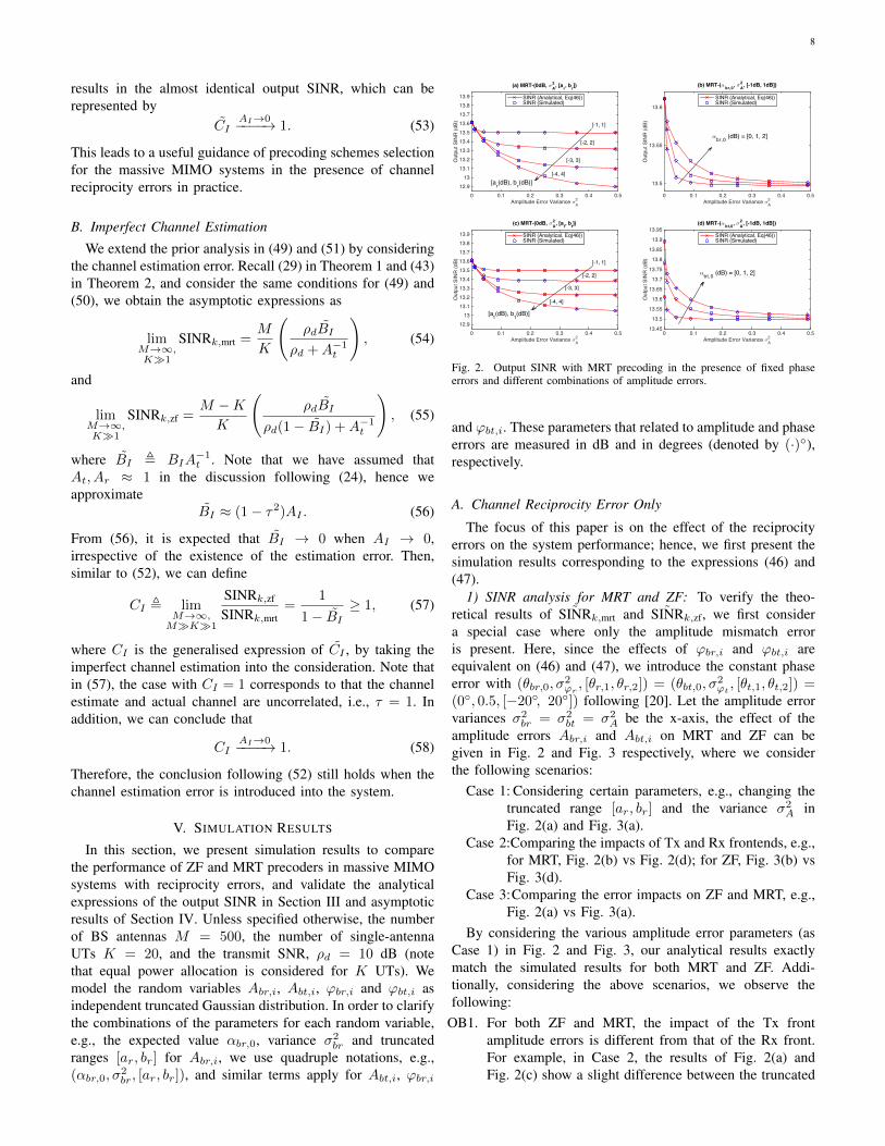
Fig. 2. Output SINR with MRT precoding in the presence of fixed phaseerrors and different combinations of amplitude errors.
and ϕbt,i. These parameters that related to amplitude and phaseerrors are measured in dB and in degrees (denoted by (·)◦),respectively.
A. Channel Reciprocity Error Only
The focus of this paper is on the effect of the reciprocityerrors on the system performance; hence, we first present thesimulation results corresponding to the expressions (46) and(47).
1) SINR analysis for MRT and ZF: To verify the theo-retical results of ˜SINRk,mrt and ˜SINRk,zf, we first considera special case where only the amplitude mismatch erroris present. Here, since the effects of ϕbr,i and ϕbt,i areequivalent on (46) and (47), we introduce the constant phaseerror with (θbr,0, σ
2ϕr, [θr,1, θr,2]) = (θbt,0, σ
2ϕt, [θt,1, θt,2]) =
(0◦, 0.5, [−20◦, 20◦]) following [20]. Let the amplitude errorvariances σ2
br = σ2bt = σ2
A be the x-axis, the effect of theamplitude errors Abr,i and Abt,i on MRT and ZF can begiven in Fig. 2 and Fig. 3 respectively, where we considerthe following scenarios:
Case 1: Considering certain parameters, e.g., changing thetruncated range [ar, br] and the variance σ2
A inFig. 2(a) and Fig. 3(a).
Case 2:Comparing the impacts of Tx and Rx frontends, e.g.,for MRT, Fig. 2(b) vs Fig. 2(d); for ZF, Fig. 3(b) vsFig. 3(d).
Case 3:Comparing the error impacts on ZF and MRT, e.g.,Fig. 2(a) vs Fig. 3(a).
By considering the various amplitude error parameters (asCase 1) in Fig. 2 and Fig. 3, our analytical results exactlymatch the simulated results for both MRT and ZF. Addi-tionally, considering the above scenarios, we observe thefollowing:
OB1. For both ZF and MRT, the impact of the Tx frontamplitude errors is different from that of the Rx front.For example, in Case 2, the results of Fig. 2(a) andFig. 2(c) show a slight difference between the truncated

9
Amplitude Error Variance σ2A
0 0.1 0.2 0.3 0.4 0.5
Out
put S
INR
(dB)
18
18.5
19
19.5
20
20.5
21
21.5
22(a) ZF-(0dB, σA
2 , [ar, br])
SINR (Analytical, Eq(47))SINR (Simulated)
Amplitude Error Variance σ2A
0 0.1 0.2 0.3 0.4 0.5
Out
put S
INR
(dB)
20.4
20.5
20.6
20.7
20.8
20.9
21
21.1
21.2(b) ZF-(αbr,0, σA
2 , [-1dB, 1dB])
SINR (Analytical, Eq(47))SINR (Simulated)
Amplitude Error Variance σ2A
0 0.1 0.2 0.3 0.4 0.5
Out
put S
INR
(dB)
18
18.5
19
19.5
20
20.5
21
21.5
22(c) ZF-(0dB, σA
2 , [at, bt])
SINR (Analytical, Eq(47))SINR (Simulated)
Amplitude Error Variance σ2A
0 0.1 0.2 0.3 0.4 0.5
Out
put S
INR
(dB)
20.5
21
21.5
22
22.5
23
(d) ZF-(αbt,0, σA2 , [-1dB, 1dB])
SINR (Analytical, Eq(47))SINR (Simulated)
[-1, 1]
[-2, 2]
[-3, 3]
αbr,0 (dB) = [0, 1, 2]
αbt,0 (dB) = [0, 1, 2]
[-4, 4][ar(dB), br(dB)]
[at(dB), bt(dB)]
[-2, 2]
[-1, 1]
[-4, 4]
[-3, 3]
Fig. 3. Output SINR with ZF precoding in the presence of fixed phase errorsand different combinations of amplitude errors.
Phase Error Variance σ2P
0 0.05 0.1 0.15 0.2 0.25 0.3 0.35 0.4 0.45 0.5
Out
put S
INR
(dB)
12.5
13
13.5
14MRT-(θ0, σP
2 , [θ1, θ2])
SINR (Analytical, Eq(46))SINR (Simulated)
(0°, σP2 , [-10°, 10°])
(0°, σP2 , [-30°, 10°])
(0°, σP2 , [-20°, 20°])
(0°, σP2 , [-30°, 30°])
(0°, σP2 , [-40°, 40°])
(10°, σP2 , [-40°, 40°]) (20°, σP
2 , [-40°, 40°])
Fig. 4. Output SINR with MRT precoding in the presence of fixed amplitudeerrors and different combinations of phase errors.
ranges of amplitude errors [ar, br] and [at, bt], whileFig. 2(b) vs Fig. 2(d) demonstrate a greater impact fromthe expected value of Tx front amplitude errors αbt,0than that from Rx front αbr,0.
OB2. It can be revealed from Case 3 that ZF is much moresensitive to the amplitude errors than MRT, as we dis-cussed in Section IV. For example, comparing Fig. 3(a)and Fig. 2(a), with the same parameters, ZF experiencesnearly 3 dB SINR loss compared to less than 1 dB lossin MRT.
Moving on to the phase reciprocity error, we fix the am-plitude errors to (αbr,0, σ
2br, [ar, br]) = (αbt,0, σ
2bt, [at, bt]) =
(0 dB, 0.5, [−1 dB, 1 dB]) as in [20]. As shown in (46)and (47), the phase errors ϕbr,i and ϕbt,i have similar ef-fect on SINR, hence, we assume (θbr,0, σ
2ϕr, [θr,1, θr,2]) =
(θbt,0, σ2ϕt, [θt,1, θt,2]) = (θ0, σ
2P , [θ1, θ2]) as shown in Fig. 4
and Fig. 5.The perfect match between the simulation results and our
analytical results can be observed from Fig. 4 and Fig. 5. We
Phase Error Variance σ2P
0 0.05 0.1 0.15 0.2 0.25 0.3 0.35 0.4 0.45 0.5
Out
put S
INR
(dB)
17
18
19
20
21
22
23ZF-(θ0, σP
2 , [θ1, θ2])
SINR (Analytical, Eq(47))SINR (Simulated)
(0°, σP2 , [-10°, 10°])
(0°, σP2 , [-40°, 40°])
(10°, σP2 , [-40°, 40°])
(0°, σP2 , [-20°, 20°])
(0°, σP2 , [-10°, 30°])
(20°, σP2 , [-40°, 40°])
(0°, σP2 , [-30°, 30°])
Fig. 5. Output SINR with ZF precoding in the presence of fixed amplitudeerrors and different combinations of phase errors.
also draw the following observations:OB3. From Fig. 5, the phase errors can cause significant
degradation of the ZF precoded system, e.g., with(0◦, 0.5, [−40◦, 40◦]), almost 6 dB loss in terms ofSINR, whereas the less severe SINR degradation (around2 dB loss) can be seen from Fig. 4 for the MRT system.
OB4. The main factors of the phase error are likely to be theerror variance σ2
P and the relative truncated range, i.e.,(θ2 − θ1), rather than the expected values θ0 (see theclosed curves between which the only difference is theincreased expected values 0◦, 10◦ and 20◦ in Fig. 4, andsimilar in Fig. 5) and the absolute values of θ1 and θ2(see the closed curves with truncated ranges [−30◦, 10◦]and [−20◦, 20◦] in Fig. 4, and with [−10◦, 30◦] and[−20◦, 20◦] in Fig. 5).
To summarise, it can be observed that the MRT precodedsystem is more tolerant to both amplitude and phase reci-procity errors compared with ZF, which is consistent with thetheoretical analysis in Section III-C.
2) When M goes to infinity: The theoretical results inTheorem 1 and 2, as well as (46) and (47) are conditionedon a large number of BS antennas M , which motivatesus to investigate the case with the asymptotic limit, i.e.,M → ∞. Again, for the sake of easy comparison withthe previous simulation results, let the same error parame-ters be considered for the transmit and receive sides. Also,we define the “Normal Level Reciprocity Error” with theamplitude errors (0 dB, 0.5, [−1 dB, 1 dB]) and phase er-rors (0◦, 0.5, [−20◦, 20◦]) as considered in [20], and “HighLevel Reciprocity Error” with (0 dB, 1, [−4 dB, 4 dB]) and(0◦, 1, [−50◦, 50◦]).
Fig. 6 demonstrates the performance of the output SINRfor ZF and MRT with different values of M . It can be con-cluded that our theoretical results accurately reflect the systemperformance in all cases, even with the not-so-large values ofM comparing to K (e.g., M ≤ 50), which corresponds tothe theory in [27]. Also, in general, ZF outperforms MRT, butagain, it is much less tolerant to reciprocity errors. Specifically,

10
Number of BS antennas M50 100 150 200 250 300 350 400 450 500
Out
put S
INR
(dB)
0
5
10
15
20
25
SINR~MRT (Analytical, Eq(46))
SINR~MRT (Simulated)
SINR~ZF (Analytical, Eq(47))
SINR~ZF (Simulated)
Perfect Channel Reciprocity
Perfect Channel Reciprocity
High Level Reciprocity Error
High Level Reciprocity Error
Normal Level ReciprocityError
Normal Level ReciprocityError
Fig. 6. Output SINR versus M in the presence of different levels of channelreciprocity errors.
ρd (dB)-10 -5 0 5 10 15 20 25 30 35 40
Out
put S
INR
(dB)
5
10
15
20
25
SINR~MRT (Analytical, Eq(46))
Upper Bound (MRT, Eq(49)) SINR~
MRT (Simulated)SINR~
ZF (Analytical, Eq(47))Upper Bound (ZF, Eq(51)) SINR~
ZF (Simulated)
Perfect Channel Reciprocity
Perfect Channel Reciprocity
High Level Reciprocity Error
High Level Reciprocity Error
Normal Level Reciprocity Error
Normal Level Reciprocity Error
Fig. 7. Output SINR versus SNR in the presence of different levels of channelreciprocity errors.
with high-level errors, more than 10 dB SINR degradation isobserved in the ZF precoded system, compared to the systemwith the ideal channel reciprocity.
Fig. 7 investigates the error ceiling effect that discussedin Section IV by increasing the transmit SNR ρd. We haveM = 500, K = 20 to satisfy the conditions of the limitthat M → ∞ and K � 1. Without the channel reciprocityerrors, the output SINR of ZF rises without an upper boundas growth of ρd, while that of MRT suffers from the inter-user interference in the high regime of ρd. The error ceilingobtained in Fig. 7 match the result in (49) for MRT, and theresult in (51) for ZF. This, in turn, leads to the conclusionthat in the high regime SNR (e.g., ρd ≥ 20 dB), both ZF andMRT suffer from the impact of the reciprocity errors, whichresults in the degraded performance that is independent ofthe transmit SNR. In addition, we observe from Fig. 6 and 7that MRT outperforms ZF in the low SNR regime or with therelatively small ratio of M/K.
ρd (dB)-10 0 10 20 30
Out
put S
INR
(dB)
2
4
6
8
10
12
14
16 (a)
SINRMRT (Analytical, Eq(29))SINRMRT (Simulated)Upper Bound (MRT, Eq(54))
ρd (dB)-10 0 10 20 30
Out
put S
INR
(dB)
0
5
10
15
20
25 (b)
SINRZF (Analytical, Eq(43))SINRZF (Simulated)Upper Bound (ZF, Eq(55))
Perfect Channel Information
Estimation Error Only
Normal level Reciprocity Error
High level Reciprocity Error
Perfect Channel Information
High level Reciprocity Error
Estimation Error Only
Normal level Reciprocity Error
Fig. 8. Output SINR versus SNR in the presence of different levels of thechannel reciprocity error and channel estimation error (τ2 = 0.1).
B. Imperfect Channel Estimation
We then extend our investigations in Fig. 7 by taking thechannel estimation error into considerations. The same condi-tions are applied as in Fig. 7, in addition with the estimationerror parameter τ2 = 0.1. As shown in Fig. 8, the close matchbetween the analytical and simulated results validates theoutput SINR expressions in (29) for MRT and (43) for ZF, aswell as the error ceiling factors in (54) and (55). Furthermore,it reveals the significant impact of the reciprocity error on theestimation error. For example, in the case that ρd = 10dB, theestimation error (with τ2 = 0.1) causes slight performancedegradation of the output SINR of the MRT precoder, around0.5dB, which is then considerably increased to 4dB whenthe high-level reciprocity error introduced. The ZF precodedsystem with imperfect channel estimation suffers more fromthe reciprocity errors, such that more than 10 dB SINR losscan be experienced in the case with the high-level reciprocityerror, compared with the degraded performance caused by theestimation error only. In addition, the results in Fig. 7 and 8can be considered in selecting suitable modulation schemesfor the practical massive MIMO system in the presence ofdifferent levels of the reciprocity error and the estimation error.
We can now generalise the conclusion at the end of Sec-tion V-A1 by taking the imperfect channel estimation intoaccount, and summarise that the MRT precoded system can bemore robust to both reciprocity and channel estimation errorscompared with the ZF precoded system.
C. Implications
In order to illustrate the implications that discussed in (52)and (57), we consider the results from Fig. 6, 7 and 8 todetermine the proper values for the conditions in (52) and(57). Here let M = 500, K = 20 and ρd = 20 dB. We alsoconsider a smaller value of the estimation error parameter,i.e., τ2 = 0.01. Since (52) and (57) are proportional to theterm AI , which is related to both amplitude and phase errors

11
σ2A = σ2
P
0 0.2 0.4 0.6 0.8 1
SIN
R C
ompa
rison
Bet
wee
n ZF
and
MR
T
100
101
102 (a)
SINRZF/MRT (Analytical)SINRZF/MRT (Simulated)C~
I (Eq(52))
σ2A = σ2
P
0 0.2 0.4 0.6 0.8 1
SIN
R C
ompa
rison
Bet
wee
n ZF
and
MR
T
100
101
102 (b)
SINRerrZF/MRT (Analytical)
SINRerrZF/MRT (Simulated)
CI (Eq(57))
SINRZF/MRT = Eq(47)/Eq(46) SINRerrZF/MRT = Eq(43)/Eq(29)
Fig. 9. Output SINR comparison of MRT and ZF.
at both Tx/Rx RF frontends, let σ2A = σ2
P to capture theaggregated variation of AI . The other parameters have thesame values of “High Level Reciprocity Error”. We then deriveSINRZF/MRT, i.e., the ratio of (47) to (46), and SINRerr
ZF/MRT,i.e., the ratio of (43) to (29), to demonstrate the output SINRcomparison between MRT and ZF, corresponding to CI in (52)and CI in (57), respectively. It can be seen that the simulation-based results in Fig. 9 are tightly matched with analyticalresults of SINRZF/MRT and SINRerr
ZF/MRT. We can also observea close match between the analytical results of SINRZF/MRT
and SINRerrZF/MRT with the asymptotic results CI and CI
respectively. Furthermore, we can conclude from Fig. 9(a)that the performance preponderance of using ZF over MRTdecreases precipitously when the level of the reciprocity errorincreases, and ends up with no gain compared to that of MRT.This conclusion holds in the case with the estimated channel asshown in Fig. 9(b). The match between our asymptotic resultin (57) and the simulation results in (b) of Fig. 9, confirms thatthe gain of ZF is highly dependent on the quality of the channelreciprocity, and this gain can be independent of the estimationerror especially with the severe reciprocity error introducinginto the system, as discussed in Section IV. Along with theobservation at the end of Section V-A2, our results in thispaper also indicate that MRT is more efficient compared to ZFin the high region of the reciprocity error, and in the relativelylow region of the reciprocity error with the low transmit SNRor with the small ratio of M/K. However, we would like tonote that further investigations, including the computationalcomplexity of different precoding schemes, may be needed toprovide a reliable comparison among different schemes.
VI. CONCLUSIONS AND DISCUSSION
In this paper, we have analysed the impact of the channelreciprocity error caused by the RF mismatches, on the per-formance of linear precoding schemes such as MRT and ZFin TDD massive MU-MIMO systems with imperfect channelestimation. Considering the reciprocity errors as multiplicativeuncertainties in the channel matrix with truncated Gaussian
amplitude and phase errors, we have derived analytical ex-pressions of the output SINR for MRT and ZF in the presenceof the channel estimation error, and analysed the asymptoticbehaviour of the system when the number of antennas at theBS is large. The perfect match has been found between theanalytical and simulated results in the cases with the practicaland asymptotically large values of the BS antennas, whichverifies that our analytical results can be utilised to effectivelyevaluate the performance of the considered system.
Our analysis has taken into account the compound effectof both reciprocity error and estimation error on the systemperformance, which provides important engineering insightsfor practical TDD massive MIMO systems, such that: 1) thechannel reciprocity error causes the error ceiling effect onthe performance of massive MIMO systems even with thehigh SNR or large number of BS antennas, which can beheld regardless of the existence of the channel estimationerror; 2) ZF generally outperforms MRT in terms of theoutput SINR. However, MRT has better robustness to bothreciprocity error and estimation error compared to ZF, thuscan be more efficient than ZF in certain cases, e.g., in thehigh region of the reciprocity error, or in the low SNR regime.This would ultimately influence the choice of the precodingschemes for massive MIMO systems in the presence of thechannel reciprocity error in practice.
Further investigations can be carried out by taking intoaccount the computational complexity and energy efficiencyof different precoding schemes, e.g., MRT, ZF, minimummean square error (MMSE) or even the non-linear dirty papercoding, along with novel compensation techniques for massiveMIMO systems suffer from the reciprocity error.
Our analysis can be generalised to large-scale fading sce-narios by considering the effect of path loss or shadowing.For example, based on the analytical and simulated results ofthe output SINR versus different transmit SNR in this paper,one possible extension is to analyse the impact of distance-dependent path loss which can be simply reflected by thereduction of the transmit power.
ACKNOWLEDGEMENT
The authors would like to acknowledge the support ofthe University of Surrey 5GIC (http://www.surrey.ac.uk/5gic)members for this work. This work has also been supportedby the European Union Seventh Framework Programme(FP7/2007-2013) under Grant 619563 (MiWaveS).
APPENDIX APRELIMINARIES ON THE TRUNCATED GAUSSIAN
DISTRIBUTION
A brief of the truncated Gaussian distribution is given here.Consider that X is normally distributed with mean µ andvariance σ2, and lies within a truncated range [a, b], where−∞ < a < b < ∞, then X conditional on a ≤ X ≤ b istreated to have truncated Gaussian distribution, which can bedenoted by X ∼ NT(µ, σ2), X ∈ [a, b]. For a given x ∈ [a, b],the probability density function can be given as [28]
f(x, µ, σ; a, b) =1
σZφ
(x− µσ
). (59)

12
The revised expected value and variance conditioned on thetruncated range [a, b] can be written as
E{X} = µ+φ(α)− φ(β)
Zσ, (60)
var (X)=σ2
[1+
αφ(α)−βφ(β)
Z−(φ(α)−φ(β)
Z
)2], (61)
where
α =a− µσ
, β =b− µσ
,Z = Φ(β)− Φ(α), (62)
φ(·) =1√2π
exp(−1
2(·)2), (63)
Φ(·) =1
2
(1 + erf
(1√2
(·)))
. (64)
APPENDIX BUSEFUL EXTENSIONS
A. Proof of Proposition 1In general, given a random variable x and its probability
function f(x), the expected value of a function of x can becalculated by
E {g(x)} =
∫ ∞−∞
f(x)g(x) dx. (65)
In this case, f(x) is given by (59) with x ∈ [a, b], and g(x) =exp(jx), thus we formulate E {g(x)} as
E {exp(jx)} =
∫ b
a
f(x, µ, σ; a, b)exp(jx) dx
=1√
2πσZ
∫ b
a
exp
(−1
2
(x− µσ
)2
+ jx
)dx
=1√
2πσZ
√π
4 12σ2
exp
(− µ2
2σ2+
(j + µ
σ2
)24 12σ2
)
× erf
√ 1
2σ2x−
j + µσ2
2√
12σ2
∣∣∣∣∣∣b
a
=1
2Zexp
(−σ
2
2+ jµ
)(erf
(√2
2
(b− µσ
)−√
2jσ
2
)
−erf
(√2
2
(a− µσ
)−√
2jσ
2
)). (66)
By invoking (62) and (64) into (66), we arrive at the result inProposition 1.
B. RemarksBased on the Proposition 1 that demonstrates a generic case
for the given x ∼ NT(µ, σ2), x ∈ [a, b], useful remarks can begiven as follows.
Remark 1. Let µ = 0 in Proposition 1, then E {exp(jx)} ofx ∼ NT(0, σ2), x ∈ [a, b] can be rewritten as
E {exp(jx)} =
exp(−σ
2
2
)erf(
b√2σ2− j σ√
2
)− erf
(a√2σ2− j σ√
2
)erf(
b√2σ2
)− erf
(a√2σ2
) . (67)
Remark 2. Let µ = 0 and a = −b in Proposition 1, thenE {exp(jx)} of x ∼ NT(0, σ2), x ∈ [−b, b] can be given as
E {exp(jx)} =exp
(−σ
2
2
)erf(
b√2σ2
)<(erf((
b√2σ2
)± j σ√
2
)).
(68)
APPENDIX CUSEFUL RESULTS
Recall (6), (8), (7) and (9), the random variables Abt,i ,Abr,i , ϕbt,i and ϕbr,i can be regarded as truncated Gaus-sian variables, whose relative parameters can be given here.Specifically, based on the preliminaries on the truncated Gaus-sian distribution in Appendix A, the amplitude-error-relatedparameters can be expressed as
αt = αbt,0 +φ(at)− φ(bt)
Ztσbt, (69)
σ2t = σ2
bt
1+atφ(at)−btφ(bt)
Zt−
(φ(at)−φ(bt)
Zt
)2 , (70)
αr = αbr,0 +φ(ar)− φ(br)
Zrσbr, (71)
σ2r = σ2
br
1+arφ(ar)−brφ(br)
Zr−
(φ(ar)−φ(br)
Zr
)2 , (72)
where at = (at − αbt,0)/σbt, bt = (bt − αbt,0)/σbt, ar =(ar −αbr,0)/σbr, br = (br −αbr,0)/σbr, Zt = Φ(bt)−Φ(at),and Zr = Φ(br) − Φ(ar). The functions φ(·) and Φ(·) aregiven in (63) and (64) respectively.
Also, the phase-error-related functions gt and gr in (29)can be expressed by applying Proposition 1 and its proof inAppendix B, as given in the following.
gt = E {exp (jϕbt,i)} = exp
(−σ2ϕt
2+ jθbt,0
)
×erf((
θt,2−θbt,0√2σ2
ϕt
)−j σϕt√
2
)−erf
((θt,1−θbt,0√
2σ2ϕt
)−j σϕt√
2
)erf(θt,2−θbt,0√
2σ2ϕt
)− erf
(θt,1−θbt,0√
2σ2ϕt
) , (73)
gr = E {exp (jϕbr,i)} = exp
(−σ2ϕr
2+ jθbr,0
)
×erf((
θr,2−θbr,0√2σ2
ϕr
)−j σϕr√
2
)−erf
((θr,1−θbr,0√
2σ2ϕr
)−j σϕr√
2
)erf(θr,2−θbr,0√
2σ2ϕr
)− erf
(θr,1−θbr,0√
2σ2ϕr
) . (74)
APPENDIX DPROOFS OF (26) AND (27)
In order to achieve the analytical expression of SINRk,mrtin Theorem 1, we calculate the normalisation parameter λmrtin (23), the expectations of signal power scaling factor Ps,mrtand the interference power scaling factor PI,mrt separately asfollowing.

13
1) λmrt: Consider the denominator inside of the square rootsign in (23), we can have
E{
tr(WmrtW
Hmrt
)}= (1−τ2)E
{tr(H∗brH
∗HTHbr
)}+τ2E
{tr(V∗VT
)}(75)
= MK((1− τ2)(α2
r + σ2r) + τ2
), (76)
where (75) is conditioned on the independence between H,Hbt, Hbr and V.
2) E {Ps,mrt}: Considering the normalised symbol powerof sk as mentioned in Section II, partial E {Ps,mrt}, i.e.,E{|hTkHbtwk,mrt|2
}, can be computed as
E{|hTkHbtwk,mrt|2
}= E
{|hTkHbt(
√1− τ2H∗brh∗k + τv∗k)|2
}= (1− τ2)E
{|hTkHbtH
∗brh∗k|2}
+ τ2E{|hTkHbtv
∗k|2}, (77)
where
E{|hTkHbtH
∗brh∗k|2}
= E
{M∑i1=1
|hi1,k|2(hbt,i1h
∗br,i1
) M∑i2=1
|hi2,k|2(h∗bt,i2hbr,i2
)}(78)
=
M∑i1=1
E{|hi1,k|4|hbt,i1 |2|hbr,i1 |2
+
M∑i2=1,i2 6=i1
|hi1,k|2|hi2,k|2hbt,i1h∗br,i1h∗bt,i2hbr,i2} (79)
= M(2(α2
t + σ2t )(α2
r + σ2r) + (M−1)α2
tα2r|gt|2|gr|2
), (80)
and similarly,
E{|hTkHbtv
∗k|2}
= M(α2t + σ2
t ). (81)
Next, by substituting (80) and (81) in (77), and invoking ρd,λmrt in (23) and the completed (77), we have (26).
3) E {PI,mrt}: By omitting the independent si for differentusers with the normalised power, partial E {PI,mrt} can be
modified as E{∣∣∣∑K
i=1,i6=k hTkHbtwi,mrt
∣∣∣2}, which is calcu-
lated as
E
∣∣∣∣∣∣
K∑i=1,i6=k
hTkHbtwi,mrt
∣∣∣∣∣∣2
=
K∑i=1,i6=k
((1−τ2)E
{|hTkHbtH
∗brh∗i |2}
+τ2E{|hTkHbtv
∗i |2}),
(82)
where
E{|hTkHbtH
∗brh∗i |2}
=
M∑j1=1
E{|hj1,k|2|hj1,i|2|hbt,j1 |2|hbr,j1 |2
+
M∑j2=1,j2 6=j1
hj1,khj2,khj1,ihj2,ihbt,j1h∗br,j1h
∗bt,j2hbr,j2} (83)
= M(α2t + σ2
t )(α2r + σ2
r). (84)
And E{|hTkHbtv
∗i |2}
can be obtained as in (81). Then ap-plying ρd, λmrt in (23) and the completed result in (82), theexpectation of PI,mrt can be given as in (27).
APPENDIX EPROOFS OF PROPOSITION 3 AND 4
To formulate the signal and interference power as well asthe output SINR in the case of ZF precoded system, thenormalisation parameter λzf can be calculated first.
1) λzf: The same conditions as in Theorem 1 are appliedwhen calculating λzf. The power constraint on Wzf can beextended as
E{
tr(WzfW
Hzf
)}= E
{tr(HHd
(HdH
Hd
)−1 (HdH
Hd
)−1Hd
)}(85)
= E{
tr((
(√
1− τ2HTHbr + τVT )
× (√
1− τ2H∗brH∗ + τV∗))−1)}
(86)
(a)≈ E
{tr((
(1− τ2)HTHbrH∗brH
∗ + τ2VTV∗)−1)}
(87)
(b)≈E
{tr
(((1−τ2
M
)HT tr(HbrH
∗br)H
∗+τ2VTV∗)−1)}
(88)
(c)=
1
(1− τ2)(α2r + σ2
r) + τ2E{
tr(W−1
sum
)}(89)
(d)=
K
(M −K)((1− τ2)(α2r + σ2
r) + τ2), (90)
where (a) is obtained due to the independence betweenthe propagation channel H and the additive estimation er-ror V. Recall the assumption that M is large, the termHTHbrH
∗brH
∗ tends to be diagonal, thus we can have (b)based on [29, Eq. (14)]. Let Wsum represent the sum of HTH∗
and VTV∗, which are two independent Wishart matrices, thenWsum has a Wishart distribution whose the degree of freedomis the sum of the degrees of freedom of HTH∗ and VTV∗
[27], thus we have (c). And (d) can be achieved based on therandom matrix theory as shown in [27]. Then we can arriveat the expression of λzf in (38).
2) E {Ps,zf}: Consider the expectation of the signalpower in (17) and recall wk,zf as the k-th column of
HHd
(HdH
Hd
)−1, we first compute the partial E {Ps,zf}, i.e.,
E{|hTkHbtwk,zf|2
}, as follows,
E{|hTkHbtwk,zf|2
}= E
{|hTkHbt[H
Hd (HdH
Hd )−1]k|2
}= E
{|hTkHbt[(
√1− τ2H∗brH∗ + τV∗)
((√
1− τ2HTHbr
+τVT )(√
1− τ2H∗brH∗ + τV∗))−1
]k|2}
(91)
≈ E{|hTkHbt[(
√1− τ2H∗brH∗ + τV∗)
×((1− τ2)HTHbrH
∗brH
∗ + τ2VTV∗)−1
]k|2},
(92)

14
where [·]k represents the k-th column of the matrix inside,and (92) can be achieved by applying (a) in deriving λzf.Consider the discussion following (90), when M is large,(HTHbrH
∗brH
∗)−1 becomes (M/tr (HbrH∗br))
(HTH∗
)−1asymptotically, and additionally, both HTH∗ and VTV∗ tendto be proportional to an identity matrix. Hence, we canapproximate (92) as
E{|hTkHbtwk,zf|2
}≈ E
{|hTkHbt[(
√1− τ2H∗brH∗ + τV∗)
×((1− τ2)tr (HbrH
∗br) + τ2M
)−1IK ]k|2
}. (93)
By using the technique in [29, Eq. (14)], and considering thethe independence between H, Hbt, Hbr and V, we have
E{|hTkHbtwk,zf|2
}≈ E
{|√
1− τ2((1− τ2)tr (HbrH
∗br) + τ2M
)−1×hTkHbtH
∗brh∗k|2}
(94)
≈ (1− τ2)α2tα
2r|gt|2|gr|2
((1− τ2)(α2r + σ2
r) + τ2)2 . (95)
Therefore, by introducing (38) and (95) into E {Ps,zf}, we canobtain (39) in Proposition 3.
3) E {PI,zf}: Based on the complete result of E {Ps,zf} inProposition 3 and λzf in (38), the expected value of partial PI,zf
omitting si (i.e., E{|∑Ki=1,i6=k
√ρdλzfh
TkHbtwi,zf|2}) can be
derived as
E
∣∣∣∣∣∣
K∑i=1,i6=k
√ρdλzfh
TkHbtwi,zf
∣∣∣∣∣∣2
=
K∑i=1,i6=k
E{|√ρdλzfh
TkHbtwi,zf|2
}(96)
(e)= ρdλ
2zf
(E{‖hTkHbtWzf‖2
}− E
{|hTkHbtwk,zf|2
})(97)
= ρdλ2zf E
{‖hTkHbtH
Hd (HdH
Hd )−1‖2
}− ρdλ2zf E
{|hTkHbtwk,zf|2
}(98)
(f)≈ ρdλ
2zf(K − 1)
M −K + 1
((α2t + σ2
t
)((1− τ2)
(α2r + σ2
r
)+ τ2)
((1− τ2)(α2r + σ2
r) + τ2)2
− (1− τ2)α2tα
2r|gt|2|gr|2
((1− τ2)(α2r + σ2
r) + τ2)2
)(99)
(g)≈ ρd(K−1)
K
(α2t +σ2
t −(1− τ2)α2
tα2r|gt|2|gr|2
(1− τ2)(α2r + σ2
r) + τ2
),
(100)
where (e) is due to the property of the ZF precoding schemeas in [10]. Based on Proposition 3 and [10], (f) is obtainedby considering the diversity order of ZF, and (g) can beachieved under the assumption of the large ratio of M/Kin the massive MIMO system. To this end, we reach theapproximated expression of E{PI,zf} in Proposition 4.
REFERENCES
[1] T. L. Marzetta, “Noncooperative cellular wireless with unlimited num-bers of base station antennas,” IEEE Trans. Wireless Commun., vol. 9,no. 11, pp. 3590–3600, Nov. 2010.
[2] E. G. Larsson, O. Edfors, F. Tufvesson, and T. L. Marzetta, “MassiveMIMO for next generation wireless systems,” IEEE Commun. Mag.,vol. 52, no. 2, pp. 186–195, Feb. 2014.
[3] F. Boccardi, R. W. Heath, A. Lozano, T. L. Marzetta, and P. Popovski,“Five disruptive technology directions for 5G,” IEEE Commun. Mag.,vol. 52, no. 2, pp. 74–80, Feb. 2014.
[4] Z. Gao, L. Dai, D. Mi, Z. Wang, M. Imran, and M. Shakir, “MmWavemassive-MIMO-based wireless backhaul for the 5G ultra-dense net-work,” IEEE Wireless Commun. Mag., vol. 22, no. 5, pp. 13–21, Oct.2015.
[5] A. Ijaz, L. Zhang, M. Grau, A. Mohamed, S. Vural, A. U. Quddus, M. A.Imran, C. H. Foh, and R. Tafazolli, “Enabling massive IoT in 5G andbeyond systems: PHY radio frame design considerations,” IEEE Access,vol. 4, pp. 3322–3339, 2016.
[6] L. Lu, G. Y. Li, A. L. Swindlehurst, A. Ashikhmin, and R. Zhang,“An overview of massive MIMO: Benefits and challenges,” IEEE J.Sel. Topics Signal Process., vol. 8, no. 5, pp. 742–758, Oct. 2014.
[7] J. Hoydis, S. ten Brink, and M. Debbah, “Massive MIMO in the UL/DLof cellular networks: How many antennas do we need?” IEEE J. Sel.Areas Commun., vol. 31, no. 2, pp. 160–171, Feb. 2013.
[8] H. Yang and T. L. Marzetta, “Performance of conjugate and zero-forcing beamforming in large-scale antenna systems,” IEEE J. Sel. AreasCommun., vol. 31, no. 2, pp. 172–179, Feb. 2013.
[9] F. Rusek, D. Persson, B. K. Lau, E. G. Larsson, T. L. Marzetta,O. Edfors, and F. Tufvesson, “Scaling up MIMO: Opportunities andchallenges with very large arrays,” IEEE Signal Process. Mag., vol. 30,no. 1, pp. 40–60, Jan. 2013.
[10] S. Wagner, R. Couillet, M. Debbah, and D. T. M. Slock, “Large systemanalysis of linear precoding in correlated MISO broadcast channelsunder limited feedback,” IEEE Trans. Inf. Theory, vol. 58, no. 7, pp.4509–4537, Jul. 2012.
[11] S. Vishwanath, N. Jindal, and A. Goldsmith, “Duality, achievable rates,and sum-rate capacity of Gaussian MIMO broadcast channels,” IEEETrans. Inf. Theory, vol. 49, no. 10, pp. 2658–2668, Oct. 2003.
[12] D. Mi, M. Dianati, S. Muhaidat, and Y. Chen, “A novel antenna selectionscheme for spatially correlated massive MIMO uplinks with imperfectchannel estimation,” in Proc. IEEE 81st Veh. Technol. Conf. (VTC), May2015, pp. 1–6.
[13] J. Choi, D. Love, and P. Bidigare, “Downlink training techniques forFDD massive MIMO systems: Open-loop and closed-loop training withmemory,” IEEE J. Sel. Topics Signal Process., vol. 8, no. 5, pp. 802–814,Oct. 2014.
[14] A. Tolli, M. Codreanu, and M. Juntti, “Compensation of non-reciprocalinterference in adaptive MIMO-OFDM cellular systems,” IEEE Trans.Wireless Commun., vol. 6, no. 2, pp. 545–555, Feb. 2007.
[15] T. Schenk, RF Imperfections in High-rate Wireless Systems: Impactand Digital Compensation. Springer Netherlands, 2008. [Online].Available: https://books.google.co.uk/books?id=nLzk11P15IAC
[16] E. Bjornson, J. Hoydis, M. Kountouris, and M. Debbah, “MassiveMIMO systems with non-ideal hardware: Energy efficiency, estimation,and capacity limits,” IEEE Trans. Inf. Theory, vol. 60, no. 11, pp. 7112–7139, Nov. 2014.
[17] R. Rogalin, O. Y. Bursalioglu, H. Papadopoulos, G. Caire, A. F. Molisch,A. Michaloliakos, V. Balan, and K. Psounis, “Scalable synchronizationand reciprocity calibration for distributed multiuser MIMO,” IEEETrans. Wireless Commun., vol. 13, no. 4, pp. 1815–1831, Apr. 2014.
[18] W. Zhang, H. Ren, C. Pan, M. Chen, R. de Lamare, B. Du, and J. Dai,“Large-scale antenna systems with UL/DL hardware mismatch: Achiev-able rates analysis and calibration,” IEEE Trans. Commun., vol. 63, no. 4,pp. 1216–1229, Apr. 2015.
[19] D. Inserra and A. M. Tonello, “Characterization of hardware impair-ments in multiple antenna systems for DoA estimation,” Journal ofElectrical and Computer Engineering, vol. 2011, p. 18, 2011.
[20] R1-100426, “Channel reciprocity modeling and performance evalua-tion,” Alcatel-Lucent Shanghai Bell, Alcatel-Lucent, 3GPP TSG RANWG1 #59, 2010.
[21] R1-110804, “Modelling of channel reciprocity errors for TDD CoMP,”Alcatel-Lucent Shanghai Bell, Alcatel-Lucent, 3GPP TSG RANWG1 #64, 2011.
[22] R1-092550, “Performance study on Tx/Rx mismatch in LTE TDD Dual-layer beamforming,” Nokia, Nokia Siemens Networks, CATT, ZTE,3GPP TSG RAN WG1 #57, 2009.

15
[23] A. Pitarokoilis, S. K. Mohammed, and E. G. Larsson, “Uplink perfor-mance of time-reversal MRC in massive MIMO systems subject to phasenoise,” IEEE Trans. Wireless Commun., vol. 14, no. 2, pp. 711–723, Feb.2015.
[24] D. Dobkin, RF Engineering for Wireless Networks: Hardware, Antennas,and Propagation. Elsevier Science, 2011.
[25] L. Zhang, A. U. Quddus, E. Katranaras, D. Wbben, Y. Qi, and R. Tafa-zolli, “Performance analysis and optimal cooperative cluster size forrandomly distributed small cells under cloud ran,” IEEE Access, vol. 4,pp. 1925–1939, 2016.
[26] Y. Lim, C. Chae, and G. Caire, “Performance analysis of massive MIMOfor cell-boundary users,” IEEE Trans. Wireless Commun., vol. 14, no. 12,pp. 6827–6842, Dec. 2015.
[27] A. M. Tulino and S. Verdu, Random Matrix Theory and WirelessCommunications. Now Publisher, 2004.
[28] N. L. Johnson, S. Kotz, and N. Balakrishnan, Continuous UnivariateDistributions, 2nd ed. New York, NY: Wiley, 1995.
[29] H. Wei, D. Wang, H. Zhu, J. Wang, S. Sun, and X. You, “Mutualcoupling calibration for multiuser massive MIMO systems,” IEEE Trans.Wireless Commun., vol. 15, no. 1, pp. 606–619, Jan. 2016.