Optimal Inflation in an Open Economy with Imperfect

Competition∗

David M. Arseneau†

Federal Reserve Board

March, 2004

Abstract

This paper uses a two-country, monetary general equilibrium model with imperfect

competition to study the optimal rate of inflation in an open economy. In contrast with

the closed economy literature, when policy is set non-cooperatively in the open economy,

the optimality of the Friedman rule is not a general result. Monetary authorities face

an incentive to use the inflation tax to gain a ”beggar-thy-neighbor” advantage over the

terms of trade. Strategic use of the inflation tax, however, results in coordination failure.

International monetary cooperation helps to mitigate this coordination failure and, as a

result, can lead to more efficient equilibria. Monetary union ensures the maximum gain

from cooperation by restoring the optimality of the global Friedman rule, placing the

world economy at the pareto frontier.

JEL Classification: E58, E61, F41, F42

Keywords: Optimal Monetary Policy, Friedman Rule, International Monetary Policy

Coordination

∗I am grateful to Eric van Wincoop and John McLaren for helpful comments on an earlier version of this

paper. In addition, the paper has benefited from presentations at Binghamton University, Texas A&M, the

Board of Governors, and the Federal Reserve Banks of Richmond and Kansas City. The views expressed in

this paper are those of the author and do not represent those of the Board of Governors or the Federal Reserve

System or other members of its staff.†Contact address: David M. Arseneau, Mail Stop 76, Division of Research and Statistics, Federal Reserve

Board, Washington, D.C. 20551. Email: david.m.arseneau@frb.gov.

1

1 Introduction

How do international linkages influence the optimal rate of inflation? Given the recent move-

ment by many central banks towards inflation targeting, the answer to this question is of growing

importance. Yet, despite rapid growth in the literature studying optimal monetary policy in

an open economy setting, surprisingly little work has been done thus far to characterize the

optimal rate of inflation.1 The reason for the lack of attention to this issue comes from the

fact that the literature that has grown out of the New Keynesian Open Economy framework es-

tablished by Obstfeld and Rogoff (1995) primarily concentrates on optimal stabilization policy.

This type of analysis focuses on the optimal monetary response to a shock, shifting attention

away from the long-run perspective of monetary policy.

This paper takes a different approach by ignoring optimal stabilization policy and concen-

trating instead on optimal inflation. Specifically, the paper develops a two-country, monetary

general equilibrium model that draws on features of Corsetti and Pesenti (2001) to extend Ire-

land (1997) to an open economy setting. It differs from existing literature in a three important

ways. First, there are no nominal rigidities in this paper.2 Second, because the focus is on

optimal inflation, the model is set in a deterministic environment. Finally, previous literature

assumes a liquidity services demand for money and models it in the utility function.3 Because

the focus of this strand of the literature has been on optimal stabilization policy, it places a

small weight on the monetary component of utility when evaluating welfare.4 In contrast,

this paper places the welfare costs of inflation at the center of the analysis by assuming a

transactions demand for money and introducing it through a cash-in-advance constraint.

Optimal inflation has been studied extensively in the closed economy literature. In models

where the transactions demand for money is the lone monetary friction the optimal rate of

inflation is given by the Friedman rule — setting the money growth rate such that the nominal

interest rate goes to zero. This finding is robust across a number of different monetary environ-

1See Lane (2001) and Sarno (2001) for general surveys of the New Keynesian Open Economy Macroeconomics

literature. Bowman and Doyle (2003) provide a survey of developments specifically related to monetary policy.2Full commitment is assumed throughout, so nominal rigidities of the form commonly used in the New

Keynesian Open Economy literature, one period ahead price-setting by all firms, adds nothing to the results.

Obviously, things change if we relax the commitment assumption or introduce staggered price-setting, but this

is not the focus of the paper.3An exception is Bachetta and van Wincoop (2000). This paper, however, focuses on the optimal exchange

rate and its influence on international trade.4For analytical convenience, it is commonplace in the New Keynesian Open Economy literature to assume

away the monetary component of utility when making welfare calculations. The justification comes from the

fact as long as the utility derived from real balances is only a small fraction of total utility, then changes in the

real component of utility will dominate changes in total utility (Obstfeld and Rogoff, 1995, chapter 10).

2

ments and, within the class of deterministic policies, when nominal price rigidities are present.5

The first main result of this paper is that, in contrast with the closed economy literature, the

optimality of the Friedman rule is not a general result when deterministic monetary policy is

set non-cooperatively in a two-country setting.6 The reason for this is that each government

has an incentive to use the inflation tax strategically in order to gain a "beggar-thy-neighbor"

advantage over the terms of trade. If the welfare gain from the positive shift in the terms

of trade outweighs the loss incurred by the introduction of a positive inflation tax, then it is

optimal to inflate away from the Friedman rule. This paper demonstrates that this is indeed

the case across a wide subset of the parameter space of the model.

To be more precise about the adjustment mechanism, anticipated inflation causes the nom-

inal interest rate to rise above zero, implying that money is dominated by bonds in rate of

return. It is well-known from the closed economy literature that agents respond by ineffi-

ciently economizing on their holdings of real cash balances, substituting out of consumption

and into leisure. Taking a fiscal interpretation, anticipated inflation acts as a tax on consump-

tion, or equivalently, and a subsidy for leisure. In a closed economy setting, the representative

agent trivially both bears the entire burden of the consumption tax and, at the same time,

enjoys the full benefit of the leisure subsidy. Accordingly, the optimal policy is to minimize

the consumption-leisure distortion by eliminating the inflation tax altogether.

This story does not necessarily hold in an open economy because leisure is a non-traded

good. Holding constant foreign inflation, higher domestic inflation creates a leisure subsidy

that primarily benefits the domestic representative agent. At the same time, the adjustment of

the exchange rate allows for expenditure shifting in both countries away from the domestically

produced good and into the foreign produced good. This expenditure shifting allows the

burden of the consumption tax to be shared equally across countries. As long as the welfare

gain from the leisure subsidy, which accrues mainly to the domestic household, outweighs the

welfare lost from the consumption tax, which is shared across countries, then it is optimal

to use domestic inflation to attempt to gain an advantage over the terms of trade. Doing

so creates a "beggar-thy-neighbor" spillover to the foreign agent. The incentive to use the

5See Chari, Christiano, and Kehoe (1996) and Correia and Teles (1999) for papers that study the optimality

of the Friedman rule across different monetary environments. Ireland (1997) and Rotemburg and Woodford

(1997) study the optimality of the Friedman rule in the presence of nominal rigidities. Dupor (2002) establishes

that, in the presence of nominal rigidities, the Friedman rule is optimal within the class of deterministic policies.

This does not necessarily hold if the policymaker randomizes.6Carlstrom and Fuerst (1999) also illustrate the suboptimality of the Friedman rule in an open economy.

Whereas they study a small open economy under perfect competition and solve for the optimal policy numer-

ically, this paper does not assume foreign activity is exogenous, allows for imperfect competition, and derives

an analytical solution for the optimal policy.

3

inflation tax strategically varies inversely with the preference weight placed on domestic goods

in the consumption aggregator implying that higher rates of inflation would be expected in

"small" economies.

There are strong similarities between the use of non-cooperative monetary policy to influence

the terms of trade and the optimal tariff argument in the international trade literature. These

similarities are well-known in open economy macroeconomics. In this paper, as in Cooper and

Kempf (2002) and Kimbrough (1991, 1993), domestic inflation influences the terms of trade

by acting as a proportional labor tax, effectively taxing foreign labor income and subsidizing

domestic labor income. In addition, despite significant differences in modeling strategies, the

results of this paper bear strong similarity to those found in Benigno (2002).7

When governments set policy independently, strategic use of the inflation tax results in

coordination failure. In light of this, the second main result of this paper is that international

monetary coordination helps to mitigate this coordination failure, and as a result, leads to

more efficient equilibria. Furthermore, an institutional arrangement such as a monetary union

places the world economy at the Pareto frontier, ensuring the maximum gain from cooperation

by restoring the optimality of the global Friedman rule.

While more in line with Canzoneri and Henderson (1991), the gains from international

monetary coordination found in this paper are in marked contrast with much of the existing

New Keynesian Open Economy literature.8 The reason for this difference, as mentioned pre-

viously, comes from the cash-in-advance modeling framework and deterministic setting used in

this paper. Together, these features highlight the welfare cost of inflation. In contrast, ex-

isting literature down plays these costs and concentrates instead on the benefits of cooperative

stabilization policy. Recent contributions that also find significant gains to cooperation for

similar reasons include Cooley and Quadrini (2003), Cooper and Kempf (2001), and Canzoneri,

Cumba, and Diba (2001). Finally, as a note of caution, these two different approaches to

evaluating the gains from cooperation invite the question, which is more relevant from a policy

perspective? This question is addressed later in the paper.

The remainder of the paper proceeds as follows. The next section describes the setup of

the model. Section 3 describes the three distortions operating in the model and discusses how

those distortions influence the optimal policy problem. Section 4 presents each government’s

7Whereas Benigno (2002) studies optimal non-cooperative stabilization policy in a model with nominal

rigidities, this paper studies optimal inflation under flexible prices. Despite these differences, the underlying

similarity of the results comes from the fact that the strategic interaction over the terms of trade is at the heart

of each analysis. In Benigno (2002) the strategic interaction comes from the incentive to use unanticipated

inflation to influence the short-run terms of trade. In this paper there is an incentive to use anticipated

inflation to influence the long-run terms of trade.8For example, Corestti and Pesenti (2001, 2002) and Obstfeld and Rogoff (2001).

4

optimization problem and solves for the optimal non-cooperative monetary policy. Three

special cases are analyzed to highlight the role of specific parameters in determining the optimal

rate of inflation in Section 5. Section 6 considers cooperation and monetary union and section

7 concludes.

2 The Model

There is perfect information in a world economy consisting of two countries, one called Home

and the other called Foreign. A representative agent in each country provides labor to a

continuum of firms residing domestically. Each firm has monopoly power over the production

of a single differentiated product sold both domestically and abroad. Money enters the model

via a cash-in-advance constraint. There are no barriers to trade so the law of one price holds and

both countries are assumed to have freely floating exchange rates. Each government controls

its respective domestic money supply by making lump-sum transfers in every period. When

setting policy, each government’s objective is to maximize the discounted lifetime utility of the

domestic representative agent.

2.1 Government

At the beginning of each period, ∀t = 0, 1, 2, . . ., the government in the Home country makesa lump sum transfer, (xt − 1)M s

t , of the Home currency to the Home representative agent by

choosing xt, the gross growth rate of the Home country money supply,M st . Foreign government

makes a lump sum transfer, (x∗t − 1)M∗st , of the Foreign currency to the Foreign representative

agent. The representative household’s money stock follows Mst+1 = xtM

st in the Home country

and M∗st+1 = x∗tM

∗st in the Foreign country. Normalize the initial period money stock in each

country, so that M s0 =M∗s

0 = 1.

2.2 Households

Agents hold two assets, domestic currency and a one-period international bond denominated in

the Home currency. The Home representative agent enters each period with nominal balances,

Mt, and bond holdings, Bt. The Foreign representative agent enters each period with nominal

balances, M∗t , and bond holdings, B

∗t . Assume that in the initial period there are zero bond

holdings in both the Home and Foreign country, B0 = B∗0 = 0.

At the beginning of the period the Home representative agent receives the nominal lump-

5

sum transfer, (xt − 1)Mst , from the Home government and then goes to the asset market.

9 In

the asset market, bonds carried over from the previous period, Bt, mature, bringing money

holdings of the Home representative agent to Mt + (xt − 1)Mst + Bt. New bonds, Bt+1, are

purchased at a price of Bt+1

Rtunits of Home currency at time t and return Bt+1 dollars at t+ 1,

where Rt is the gross nominal interest rate between time t and t + 1. Similarly, the Foreign

currency price of the bond is 1St

B∗t+1Rt

units of foreign currency at time t, where St is the nominal

exchange rate (Home price of a unit of Foreign currency). Upon conclusion of trade in asset

markets the Home representative agent is left with Mt + (xt − 1)M st + Bt − Bt+1

Rtin Home

currency cash balances.

The representative household in each country then splits into a worker and a shopper. The

shopper takes the remaining cash balances to the goods market. Assuming the existence of

a frictionless foreign exchange market so that the representative shopper in either country can

purchase both domestic and foreign goods, the Home shopper purchases a consumption basket,

ct , the price of which is given by Pt. The Home shopper faces the following cash-in-advance

constraint 10

Ptct ≤Mt + (xt − 1)M st +Bt − Bt+1

Rt. (1)

Meanwhile, the worker in the Home country supplies lt (h) , ∀h ∈ [0, 1] units of labor toindividual firms residing in the Home country. Firms use labor for production of a differentiated

product also indexed by h. Foreign workers supply l∗t (f) , ∀f ∈ [0, 1] units of labor to firmsresiding in the Foreign country. Define the following aggregators for Home and Foreign labor,

respectively: lt =R 10lt (h) dh and l∗t =

R 10l∗t (f) df .

At this point production takes place, exchange occurs, and the goods and labor markets

both clear. Workers receive a nominal wage denominated in the domestic currency, denotedWt

and W ∗t for Home and Foreign workers, respectively. Each firm pays out monopoly profits to

domestic households in the form of a dividend. The dividend is denominated in the domestic

currency, denotedDt (h) andD∗t (f) for the representative firm in the Home and Foreign country,

respectively. Households in each country use unspent cash, wages, and dividends to accumulate

domestic money to take into the next period, Mt+1 and M∗t+1.

9Note that the lump sum transfer, (xt − 1)Mst , depends on the money holdings of the typical agent through

money supply,Mst . Therefore, all Home agents receive an identical lump sum transfer regardless of the quantity

of money they choose to bring into the period, Mt.10This is different from the CIA constraint used in Helpman (1981) in which domestic agents hold both

domestic and foreign currencies and therefore face two CIA constraints. The assumption of a single CIA

constraint is made here to avoid issues that arise regarding currency substitution.

6

The budget constraint for the Home representative household is

Ptct +Bt+1

Rt+Mt+1 ≤Mt + (xt − 1)Ms

t +Bt +

Z 1

0

Dt (h) dh+Wtlt. (2)

2.2.1 Preferences, Consumption Indexes, Prices, and the Terms of Trade

Preferences of the representative Home household are defined over consumption of an aggregate

consumption basket and labor.

Ut =∞Xt=0

βtµ

1

1− σc1−σt − lt

¶, where 0 < β < 1 and 0 < σ < 1. (3)

The Home aggregate consumption basket consists of differentiated products produced by

firms residing in both the Home and Foreign country. Define an index of per capita consumption

of the Home and Foreign commodity bundles as follows

ct = cγH,tc1−γF,t , where 0 < γ < 1. (4)

The Home commodity bundle, cH,t, aggregates consumption by the Home agent of all dif-

ferentiated products produced by firms residing in the Home country. Similarly, the Foreign

commodity bundle, cF,t, aggregates consumption by the Home agent of all differentiated prod-

ucts produced by firms residing in the Foreign country. Consumption of the Home and Foreign

commodity bundles are defined as follows

cH,t =

µZ 1

0

ct (h)θ−1θ dh

¶ θθ−1

and cF,t =

µZ 1

0

ct (f)θ−1θ df

¶ θθ−1, θ > 1. (5)

There exists a Foreign counterpart to equation 3 defining the utility of the Foreign represen-

tative agent, U∗t . Also, similar expressions to equations 4 and 5 define an index of per capita

consumption for the Foreign agent, c∗t , and Foreign consumption of the Home and Foreign

commodity bundles, denoted c∗H,t and c∗F,t, respectively.

The functional form used for preferences implies the elasticity of intertemporal substitution

is given by 1σ. The consumption aggregator used in equation 4 is Cobb-Douglas implying unit

elasticity of substitution between Home and Foreign commodity bundles.11 As in Benigno

(2002), the preference weight placed on the Home commodity bundle in the Home consumption

aggregator, γ, is interpreted as the "economic" size of the Home country. Finally, the elasticity

of substitution between goods produced within a given country is constant at θ > 1.

11As noted in Corsetti and Pesenti (2001), because the elasticity of intertemporal substitution exceeds the

elasticity of intratemporal substitution these functional forms imply that the Home and Foreign commodity

bundles are compliments.

7

The Home currency consumption-based price index aggregates over the subindexes for the

price of the Home and Foreign goods in the Home country denominated in the Home currency.12

Pt =1

γWP γH,tP

1−γF,t , where γ

W = γγ (1− γ)1−γ (6)

PH,t =

µZ 1

0

Pt (h)1−θ dh

¶ 11−θ

and P ∗F,t =µZ 1

0

P ∗t (f)1−θ df

¶ 11−θ

(7)

There exists a Foreign counterpart to equation 6 defining the Foreign currency consumption-

based price index, P ∗t . There are no barriers to trade in the model so the law of one price

holds across individual goods, Pt (h) = StP∗t (h), ∀h ∈ [0, 1] and Pt (f) = StP

∗t (f), ∀f ∈ [0, 1].

Furthermore, Home and Foreign agents are assumed to have identical preferences, implying

that consumption based purchasing power parity (PPP) holds across the price of Home and

Foreign commodity bundles, PH,t = StP∗H,t and PF,t = StP

∗F,t. Finally, by equation 6, PPP

holds across the aggregate price index in each country.

Pt = StP∗t (8)

At this point it is useful to define the Home country terms of trade, ToTt =PH,tStP∗F,t

, as the

price of exports relative to the price of imports, denominated in the Home currency.

2.2.2 Household Optimization

Nominal variables in the cash-in-advance constraint and the budget constraint are scaled by

the domestic money supply. Let lower case letters denote normalized variables, so for generic

Home nominal variable, Zt, its normalization is defined as zt = ZtMstand its Foreign counterpart

as z∗t =Z∗tM∗st.

This allows the Home representative household’s normalized cash-in-advance constraint to

be expressed as13

ptct ≤ mt + (xt − 1) + bt − bt+1xtRt

. (9)

The normalized budget constraint is as follows

ptct +bt+1xtRt

+mt+1xt ≤ mt + (xt − 1) + bt +

Z 1

0

dt (h) dh+ wtlt. (10)

Using this notation, the representative household in the Home country takes as given the

sequences pH,t (h) , p∗F,t (f) , dt (h) , wt, Rt, xt, x

∗t and chooses quantities cH,t (h) , cF,t (f) , lt,

12The consumption-based price index for the Home country is defined as the minimum expenditure required

to purchase one unit of the Home aggregate consumption bundle, given the prices of the Home and Foreign

goods.13In equations 9 and 10 we make use of the fact that Bt+1

Mst

1Rt= bt+1xt

1Rt, where xt =

Mst+1

Mst.

8

mt+1, bt+1 to maximize 3 subject to 4, 5, 9, and 10. The representative household in the

Foreign country solves a similar problem.

2.3 Firms

Profit maximizing firms in both the Home and Foreign country set prices in every period and

produce output according to a linear production technology that requires one unit of labor to

produce one unit of output. Let Yt (h) = lt (h), ∀h ∈ [0, 1] denote the output of a typical firmresiding in the Home country. Similarly, let Y ∗t (f) = l∗t (f), ∀f ∈ [0, 1] denote the output of atypical firm residing in the Foreign country. Aggregating output over all domestic firms yields

total output produced in the Home and Foreign country, denoted Yt and Y ∗t respectively.

Yt =

Z 1

0

Yt (h) dh, and Y ∗t =Z 1

0

Y ∗t (f) df

After production and exchange, each firm makes its wage payment to the worker and pays

out profits to the representative household in the form of a dividend, denoted dt (h) , ∀h ∈ [0, 1]and d∗t (f) , ∀f ∈ [0, 1] for firms residing in the Home and Foreign country, respectively.The only decision made by firms in any given period is to choose period t prices to maximize

profit subject to demand. Given the linear production technology, the representative firm’s

profits equals price minus wage times quantity sold, where shoppers in the global goods market

determine quantity sold. The normalized profit function for a typical producer in the Home

country is as follows.

dt (h) = (pH,t (h)− wt) cWt (h) (11)

Global demand functions for the representative good produced in the Home and Foreign

country, respectively, are given by the following.

cWt (h) = γ

·pt (h)

pH,t

¸−θ µpH,t

pt

¶−1(ct + c∗t ) , and (12)

cWt (f) = (1− γ)

·pt (f)

pF,t

¸−θ µpF,tpt

¶−1(ct + c∗t )

Taking as given the sequences pH,t (i) ∀i 6= h ∈ [0, 1] , p∗F,t (f) ∀f ∈ [0, 1] , wt, xt, x∗t , the

representative firm in the home country sets the price, pH,t (i), to maximize the dividend, dt (i) ,

paid to the representative household. Foreign firms solve a similar problem.

2.4 The Competitive Equilibrium Under Imperfect Competition

The Home and Foreign government each commit to a monetary policy plan in the initial

period, t = 0. Let x = {xt|t = 0, 1, 2, . . .} denote the Home monetary policy plan and

9

x∗ = {x∗t |t = 0, 1, 2, . . .} denote the Foreign monetary policy plan. Taken together, x and

x∗ constitute world monetary policy. Once the world monetary policy is revealed, the global

private sector responds with a sequence of prices and quantities that constitute a competitive

equilibrium under imperfect competition at every point in time.

Definition 1 In a monopolistically competitive equilibrium: taking as given x and x∗, (i.) firmsresiding in the Home and Foreign country set prices to maximize profit in every period; (ii.) the

Home and Foreign representative agents maximize utility in every period; and (iii.) all markets

clear in every period.

For any given world monetary policy announcement, when the market clearing conditions

are imposed, the efficiency conditions of households and firms can be manipulated into a set of

conditions governing real quantities that must hold in any long-run monopolistically competitive

equilibrium.14

c =

µαβ

θ − 1θ

1

xγx∗1−γ

¶ 1σ

, c∗ =µα∗β

θ − 1θ

1

xγx∗1−γ

¶ 1σ

(13)

l =1

γW

µ1

ToT

¶1−γc, and l∗ =

1

γW(ToT )γ c∗ (14)

ToT =

µγ

1− γ

¶σx

x∗(15)

Where α = γ ((1− γ) /γ)(1−σ)(1−γ) and α∗ = (1− γ) (γ/ (1− γ))(1−σ)(1−γ) . The intuition

behind these equations is left to the following section.

3 Three Distortions

Before discussing the choice of optimal policy it is useful to provide a description of the three

distortions operating in the economy and illustrate how each influences government’s policy

decision. Following Khan, King, andWolman (2003) andWolman (2001), the perfectly efficient

outcome is referred to as the first-best. From the perspective of the Home country, in the first-

best the real wage is equal to the marginal product of labor in the production of one unit of

the aggregate consumption basket,³wp

´fb= ∂c

∂cH

∂cH∂l, and the representative household in each

country chooses quantities such that the real wage equals the marginal rate of substitution

between consumption and leisure,³UlUc

´fb=³wp

´fb.

14Details of the solution for the competitive equilibrium are contained in a technical appendix available from

the author upon request.

10

The three distortions either cause the real wage, the marginal product of labor, or both

simultaneously to deviate from the first best. Each government’s policy problem, therefore,

reduces down to using domestic money growth to minimize the cumulative welfare effects of

each of these three distortions, taking as given monetary policy in the foreign country.

3.1 Monetary Distortion

The monetary distortion operates on the wedge between the marginal rate of substitution and

the real wage, UlUc

< wp. It can be isolated by assuming γ = 1 and θ→∞.

Ul

Uc

= β1

x;w

p= 1

For any x > β, anticipated inflation pushes the net nominal interest rate above zero, causing

money to be dominated in rate of return. Agents respond by economizing on real balance hold-

ings, substituting out of consumption and into leisure. The resulting monetary distortion forces

consumption suboptimally low and leisure suboptimally high relative to the first-best. Taking

a fiscal interpretation, inflation distorts the consumption/leisure decision by taxing consump-

tion, or, equivalently, subsidizing leisure. In the closed economy under perfect competition an

optimizing government eliminates the monetary distortion by implementing the Friedman rule,

x = β, equating the rate of return on money and bonds.

3.2 Monopolistic Distortion

The monopolistic distortion drives a wedge between the real wage and the marginal product of

labor, wp<³wp

´fb, and can be isolated by assuming γ = 1 and x = β.

Ul

Uc

=w

p=1

Φ

Monopolistically competitive firms set price as a markup over marginal cost, where we

introduce the notation Φ = θθ−1 . Taking a fiscal interpretation, the markup can be thought

of as a tax on labor income in order to limit production allowing firms to maximize monopoly

profits. Ideally, an optimizing government desires to use monetary policy to correct for this

distortion by using deflation to subsidize consumption, or, equivalently, tax leisure, such that

firms produce output at the first-best. However, such a rate of deflation, x = β 1Φ< β, would

push the nominal interest rate below zero, which is not possible due to arbitrage. As a result,

the zero lower bound on the nominal interest rate implies that government can never eliminate

the monopolistic distortion in an equilibrium with commitment.

11

3.3 Strategic Terms of Trade Distortion

The strategic terms of trade distortion operates simultaneously on both the wedge between

the marginal rate of substitution and the real wage and the wedge between real wage and the

marginal product of labor. Its effects are easiest to isolate by assuming perfect competition in

a symmetric open economy, θ →∞, γ = 12.

Ul

Uc

=U∗lU∗c

=1

2β

1√xx∗

w

p=1

2

rx

x∗;w∗

p∗=1

2

rx∗

x

Some algebra shows that for the real wage to equal the marginal rate of substitution the

following conditions must hold in the Home and Foreign countries, respectively.

1 = β1

x; 1 = β

1

x∗

Independent of the actions of the Foreign government, the Home government can eliminate

the wedge between the real wage and the marginal rate of substitution by implementing the

Friedman rule. However, when policy is set non-cooperatively control of the domestic money

supply gives the Home government a degree of monopoly power over the relative price of Home-

produced goods on international markets. The Home government has an incentive to exploit

this monopoly power by committing to a higher level of inflation than prevails in the Foreign

country. Doing so creates two effects. First, it creates a favorable shift in the terms of trade that

raises the real wage of Home workers relative to Foreign workers. Second, it reintroduces the

monetary distortion. Thus, in an open economy each government acting independently faces

a trade-off between the costs and benefits of anticipated inflation. An optimizing government

desires to set domestic money growth such that the marginal benefit of inflation is exactly offset

by the marginal cost.

3.3.1 A Fiscal Interpretation of the Policy Trade-off

The intuition behind the open economy policy trade-off is best understood by taking a fiscal

interpretation of anticipated inflation and comparing the closed economy case to the open

economy case. In a closed economy, the representative agent trivially bears the entire burden

of the consumption tax generated by anticipated inflation, or, equivalently, enjoys the entire

benefit of the leisure subsidy. The welfare loss from the reduction in consumption outweighs

the welfare gain from increased leisure, so anticipated inflation is always costly. An optimizing

government desires to minimize these costs by implementing the Friedman rule, setting the

nominal interest rate equal to zero, thereby removing the monetary distortion.

12

This story does not carry over to the open economy setting because leisure is a non-traded

good. Holding constant Foreign inflation, higher relative inflation in the Home country in-

fluences the consumption/labor choice of the Home representative agent choice through two

separate and opposing channels. First, as in the closed economy case, anticipated inflation

creates a tax on aggregate consumption by pushing the nominal interest rate above zero, rein-

troducing the monetary distortion. However, in contrast with the closed economy, international

trade allows the burden of the aggregate consumption tax to be shared equally by the represen-

tative agents in both countries. This can been seen using the Home and Foreign counterparts

to equation 13 to note that domestic inflation lowers the level of aggregate consumption in both

countries in constant proportion.

c

c∗=

γ

1− γ

At the same time, higher relative inflation in the Home country drives up the relative real

wage of Home workers through a favorable shift in the terms of trade. From a fiscal perspective,

the increase in the relative real wage can be thought of as a tax levied by the Home government

on Foreign labor income that is used to subsidize Home labor income. Leisure is a non-traded

good so the welfare effects cannot be traded across countries. Therefore, even though Home

and Foreign households continue to consume in equal proportion, the burden of labor input into

production is shifted away from Home workers and onto Foreign workers. This can been seen

using the Home and Foreign counterparts to equation 14 to derive an expression for relative

labor input across the two countries.

l

l∗=

γ

1− γ

1

ToT

From the Home government’s perspective, as long as the increase in utility resulting from

the leisure subsidy outweights the decrease in utility resulting from the tax on aggregate con-

sumption, it is optimal to impose a positive inflation tax by inflating away from the Friedman

rule. Doing so produces a ”beggar-thy-neighbor” welfare spillover in the sense that the Foreign

agent bears an equal share of the tax on aggregate consumption, but, due to the adverse shift

in the terms of trade, does not gain the full benefit of the leisure subsidy enjoyed by the Home

agent.

The incentive to use the inflation tax strategically depends on the ability to redistribute

the burden of labor used in production away from the domestic worker and onto the foreign

worker. The strength of this redistributive channel is governed by two parameters: the elasticity

of intertemporal substitution, 1σ, and the preference weight placed on domestic goods in the

consumption aggregator, γ. The role of each of these will be examined in greater detail in

13

section 5.

4 The Optimal Non-cooperative Rate of Inflation

In both countries, the policy space is bounded below, so that xt, x∗t ∈ [β,∞]. The lower

bound is imposed so the net nominal interest rate (1−Rt) never goes below zero. The optimal

non-cooperative world monetary policy is defined as a Nash-Ramsey world monetary policy.

Definition 2 The Nash-Ramsey world monetary policy is the collection of Home and Foreignmoney growth rates that, conditional on the optimal response by the global private sector, satisfy

the following: (i.) taking as given x∗, the Home government chooses x to maximize the dis-

counted lifetime utility of the Home representative agent, and (ii.) taking as given x, the Foreign

government chooses x∗ to maximize the discounted lifetime utility of the Home representative

agent.

The Home government’s problem is to set the sequence of domestic money growth rates

to maximize 3 subject to 13, 14, and xt ∈ [β,∞] , taking as given Foreign monetary policy.The Foreign government solves a similar problem taking as given monetary policy in the Home

country.

Absent constraints on the policy space, each government would like to set money growth

at the point at which the marginal benefit of inflation exactly offsets the marginal cost. The

solution to this problem is given by x = β 1ΦD in the Home country and x = β 1

ΦD∗ in the

Foreign country, where for convenience we introduce the notation D =³1 + 1−γ

γσ´, and D∗ =³

1 + γ1−γσ

´. Whether or not each government will be able to achieve this rate of money growth

given the constraints on the policy space depends on the relative size of Φ and D in the Home

country and Φ and D∗ in the Foreign country. Table 1 breaks up the parameter space of the

model into four distinct regions depending on the relative size of Φ, D, and D∗ and summarizes

the Nash-Ramsey world monetary policy in each of these regions.

Figures 1 through 3 give a better idea about how the Nash-Ramsey world monetary policy

varies across the parameter space. Figure 1 considers the symmetric open economy, γ = 12,

and demonstrates that D = D∗ = (1 + σ) tends to get large relative to Φ as σ and θ get larger.

Figure 2 illustrates the relationship between x = x∗, D = D∗ = (1 + σ) , and Φ. In the top

panel the parameterization is such that Φ > D. The optimal rate of inflation in the open and

closed economy coincide at the Friedman rule. However, in panel B when σ passes a certain

threshold (σ = 0.09 when θ = 12 and σ = 0.2 when θ = 12), Φ < D and optimal inflation

is above the Friedman rule in the symmetric open economy. Finally, figure 3 considers the

14

asymmetric open economy. Holding constant the markup and the intertemporal elasticity of

substitution, as the preference weight placed on domestic goods in the consumption aggregator

falls, there is a stronger incentive to use the inflation tax to manipulate the terms of trade.

Taken together, these figures highlight the fact that across the majority of the parameter

space of the model, in contrast with the closed economy literature, the Friedman rule is sub-

optimal when monetary policy is set non-cooperatively in an open economy setting.

5 Three Special Cases

This section considers three special cases that highlight the role of the markup, Φ, the intertem-

poral elasticity of substitution, 1σ, and the preference weight placed on domestic goods in the

consumption aggregator, γ, in determining the optimal non-cooperative rate of inflation.

5.1 The Closed Economy, γ = 1

Although the results of the closed economy case are well known in the literature they are

restated here to serve as a benchmark of the open economy results. The closed economy can

be replicated by assuming that agents in the Home country put full preference weight on the

Home commodity bundle in the consumption aggregator, γ = 1. In this case, the first-best is

given by³UlUc

´fb=³wp

´fb= 1

There is no benefit to inflation because, trivially, government cannot influence the real wage

through the terms of trade. Therefore, there is no policy tradeoff. Inflation serves only to push

the nominal interest rate above zero driving a wedge between the marginal rate of substitution

between consumption and leisure and the real wage. The Friedman rule, x = β, eliminates

this wedge.

Perfect Competition, θ → ∞ With perfectly competitive product markets the Friedman

rule achieves the first-best, or perfectly efficient, outcome by eliminating the monetary distor-

tion, so that UlUc= w

p= 1.

Imperfect Competition, θ <∞ Under imperfect competition, the markup distortion drives

a wedge between the real wage in the monopolistic equilibrium and its perfectly efficient level,wp< 1. In this case, the Friedman rule produces a second-best outcome, so that Ul

Uc= w

p< 1.

This is the best government can do under commitment given the underlying monopolistic

distortion.

15

5.2 The Symmetric Open Economy, γ = 1/2

The optimal non-cooperative policy in absence of constraints on the policy space is that which

sets the marginal benefit of inflation equal to the marginal cost, x = x∗ = β 1ΦD where D =

(1 + σ). When the constraints on the policy space are imposed it must be the case that x,

x∗ ≥ β, which requires D ≥ Φ. When this condition does not hold the Freidman rule is the

next best alternative.

Perfect Competition, θ →∞ The only circumstance under which the Friedman rule is the

optimal non-cooperative policy is when preferences are linear (σ = 0, so that Φ = D = D∗ = 1).

In this case, it produces a first-best outcome where³UlUc

´fb=³wp

´fb=³U∗lU∗c

´fb=³w∗p∗

´fb= 1

2.

As the elasticity of intertemporal substitution falls (as σ gets larger) D > 1. Agents become

less willing to substitute intertemporally an more willing to substitute between consumption

and leisure. As a result, relative labor input becomes more sensitive to movements in the terms

of trade. This drives up the potential welfare gain from the relative labor income tax making

it more attractive to inflate away from the Friedman rule, even at the cost of reintroducing the

monetary distortion.

Due to symmetry, however, neither government ever gains an advantage over the terms of

trade in equilibrium. The relative real wage remains unchanged and the monetary distortion

forces the marginal rate of substitution below the real wage. In this case, the optimal non-

cooperative policy produces a second-best outcome where UlUc=

U∗lU∗c

< wp= w∗

p∗ =12.

Imperfect Competition, θ < ∞ Introducing imperfect competition increases the costs of

inflation and in doing so widens the parameter space under which the Friedman rule is the

optimal non-cooperative policy. When D = D∗ ≤ Φ, the costs associated with exacerbating

the monetary distortion outweigh the potential benefits of gaining an advantage over the terms

of trade. In fact, when D = D∗ < Φ each government desires to push inflation even lower

than the Friedman rule in order to generate a consumption subsidy that would force firms to

produce output closer to its efficient level, even at the cost of worsening the terms of trade.

Governments are prevented from doing this by the zero lower bound and the Friedman rule

produces a second-best outcome where UlUc=

U∗lU∗c= w

p= w∗

p∗ < 12.

On the other hand, when D = D∗ > Φ, the potential welfare gain from the favorable

shift in the terms of trade makes it optimal to impose a positive inflation tax. Under perfect

symmetry, neither country will ever gain an advantage over the terms of trade in equilibrium

and inflation only serves to drive the real wage below the marginal product of labor. In this

case, x = x∗ = β 1ΦD produces a third-best outcome where Ul

Uc=

U∗lU∗c

< wp= w∗

p∗ < 12.

16

5.3 The Small Open Economy, 0 < γ < 1/2

In the asymmetric world economy, the optimal non-cooperative policy in absence of constraints

on the policy space is given by x = β 1ΦD, where D =

³1 + 1−γ

γσ´and x∗ = β 1

ΦD∗, where

D∗ =³1 + γ

1−γσ´. As noted previously in the description of figure 3, as a country gets

smaller in "economic" size there is a stronger incentive to commit to a higher rate of inflation.

The reason for this is that when a country is small its goods make up only a small portion

of aggregate consumption. Government can therefore achieve a large redistribution of the

burden of labor used in production away from the Home worker and onto the Foreign worker

by imposing a positive inflation tax that has only a small effect on aggregate consumption.

6 Cooperation and Monetary Union

Strategic use of the inflation tax results in coordination failure that reduces overall welfare.

This coordination failure can be eliminated if both governments agree to cooperate when setting

monetary policy. Concentrating first on the symmetric open economy case, if the elasticity

of intertemporal substitution and the markup are sufficiently large such that Φ ≥ D = D∗,

then there exist no gains from cooperation. In this part of the parameter space the optimal

inward-looking policy self-enforces cooperation. However, if Φ < D = D∗, the gains from

cooperation can be quite large.

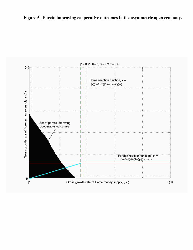
Figure 4 illustrates this point for the parameterization β = 0.95, σ = 0.9, θ = 6. The

shaded region shows the entire set of Pareto improving cooperative outcomes. An institutional

arrangement to that ensures the maximum welfare gain from cooperation is to form a monetary

union, implying St = 1, ∀ t = 0, 1, 2 . . .. In this case, each government sets policy strictly

inward-looking and the optimality of the Friedman rule is restored, moving the world economy

to the Pareto efficient frontier. Table 2 demonstrates the gains from monetary union as

opposed to the non-cooperative equilibrium under various parameterizations. Welfare gains

from monetary union are increasing in θ and decreasing in σ. For close to log preferences the

welfare gains range from 3.4% to 5.3% of period utility.

The asymmetric open economy highlights the role of the preference weight placed on do-

mestic goods in the consumption aggregator in determining the welfare gains from cooperation.

Setting γ = 0.25, the shaded region on figure 5 shows the set of Pareto improving cooperative

outcomes. Again, forming a monetary union ensures the maximum gains from cooperation

by restoring the optimality of the Friedman rule. Table 3 demonstrates that the gains from

monetary union under various parameterizations. Generally speaking, larger countries tend to

gain more from a monetary union.

17

At this point a quick comment is in order regarding the policy implications of these results.

A solid arguement can be made that the appropriate way to think about the gains from mon-

etary union is in the context of the short-run stabilization role for monetary policy. Indeed,

this is precisely the focus of much of the existing literature. Because it is set in a deterministic

environment this model is silent on this issue and, as a result, the gains from cooperation found

here should be interpreted with care.

7 Conclusions

This paper analyzed the optimal inflation tax in an open economy with imperfect competition

when the transactions demand for money is the lone monetary friction. In contrast with the

closed economy literature, the optimality of the Friedman rule is not a general result. When

monetary policy is set non-cooperatively in a two-country setting there is an incentive to use

inflation as a proportional labor tax to gain an advantage over the terms of trade. The

incentive to use the inflation tax strategically depends on the ability to redistribute the burden

of labor used in production away from the domestic worker and onto the foreign worker. The

strength of this redistributive channel grows as the intertemporal elasticity of substitution falls

and as a country gets smaller in economic size. Lastly, the paper documents potentially

large gains from cooperation and demonstrates that forming a monetary union puts the world

economy on the Pareto frontier by restoring the optimality of the Friedman rule. These policy

implications, however, should be interpreted with care because the model does not address

cooperative stabilization policy.

18

References

[1] Bachetta, P. and E. van Wincoop (2000), "Does Exchange Rate Stability Increase Trade

and Welfare?" American Economic Review, 2000, 90(5), 1093-1109.

[2] Benigno, P. (2002), ”A Simple Approach to International Monetary Policy Coordination”

Journal of International Economics, 57, 177-196.

[3] Benigno, G. and Benigno, P. (2002), ”Price Stability in Open Economies” NYU and LSE

working paper.

[4] Bowman, D. and B. Doyle (2003), ”New Keynesian Open Economy Models and Their

Implications for Monetary Policy,” Federal Reserve Board of Governors working paper No.

762.

[5] Canzoneri, M., Cumby, R., and Diba, B. (2001), ”The Need for International Policy Co-

ordination: What’s Old, What’s New, What’s Yet to Come?” Unpublished manuscript,

Georgetown University.

[6] Canzoneri, M. and D. Henderson (1991), ”Monetary Policy Games in Interdependent

Economies” MIT Press, Cambridge, MA.

[7] Carlstrom, C.T. and T. S. Fuerst (1999), "Optimal Monetary Policy in a Small Open

Economy: A General Equilibrium Analysis, " Federal Reserve Bank of Cleveland working

paper No. 9911.

[8] Chari, V.V., Christiano, L.J., and Kehoe, P.J. (1996), ”Optimality of the Friedman Rule

in Economies with Distorting Taxes” Journal of Monetary Economics, 37, 203-223.

[9] Cooley, T. and Quadrini, V. (2003), ”Common currencies vs. Monetary Independence”,

Forthcoming Review of Economic Studies.

[10] Cooper, R. and H. Kempf (2003), ”Commitment and the Adoption of a Common Currency”

Forthcoming International Economic Review.

[11] Correia, I and Teles, P. (1999), ”The Optimal Inflation Tax” Review of Economic Dynam-

ics, 2, 325-346.

[12] Corsetti, G. and P. Pesenti (2001), ”Welfare and Macroeconomic Interdependence” Quar-

terly Journal of Economics, 116(2), 421-445.

19

[13] Devereux, M. B. and Engle, C. (2003), "Monetary Policy in the Open Economy Revisited:

Price Setting and Exchange Rate Flexibility," Review of Economic Studies, 70, 765-783.

[14] Dupor, B. (2002), ”Optimal Random Monetary Policy with Nominal Rigidity” Wharton

School, University of Pennsylvania working paper.

[15] Helpman, E. (1981), "An Exploration in the Theory of Exchange Rate Regimes" Journal

of Political Economy, 89(8), 865-890.

[16] Ireland, Peter N. (1997), ”Sustainable Monetary Policies” Journal of Economic Dynamics

and Control, 22, 87-108.

[17] Khan, A., R. King, and A. Wolman (2000), "Optimal Monetary Policy" Federal Reserve

Bank of Richmond Working Paper No. 00-10.

[18] Kimbrough, K. (1991), ”Optimal Taxation and Inflation in an Open Economy” Journal of

Economic Dynamics and Control, 15, 179-196.

[19] Kimbrough, K. (1993), ”Optimal Monetary Policies and Policy Interdependence in the

World Economy” Journal of International Money and Finance, 12, 227-248.

[20] Lane, P.R. (2001), ”The New Open Economy Macroeconomics: A Survey”, Journal of

International Economics, 54, 235-266.

[21] Obstfeld, M., and K. Rogoff (1995), ”Exchange Rate Dynamics Redux” Journal of Political

Economy, 103, 624-660.

[22] Obstfeld, M., and K. Rogoff (1996), Foundations of International Macroeconomics. MIT

Press, Cambridge, MA.

[23] Rogoff, K. (2003),

[24] Rotemburg, J. and Woodford, M. (1997), ”An Optimization-Based Econometric Frame-

work for the Evaluation of Monetary Policy” in NBER Macroeconomics Annual (Ben

Bernanke and Julio Rotemberg, eds.) MIT Press: Cambridge, Massachuesetts.

[25] Sarno, L. (2001), ”Toward a New Paradigm in Open Economy Modeling: Where Do We

Stand?” Federal Reserve Bank of St. Louis Review, May/June, 21-36.

[26] Wolman, A. (2001), "A Primer on Optimal Monetary Policy with Staggered Price-Setting"

Federal Reserve Bank of Richmond Economic Quarterly, 87(4), 27-52.

20

Table 1. Nash-Ramsey world monetary policy *D>Φ *D>Φ

β== *xx β=x ; ** 1 DxΦ

= β D>Φ

1* == RR 1=R ; ** 1 DRΦ

=

DxΦ

=1β ; β=*x Dx

Φ=

1β ; ** 1 DxΦ

= β D≤Φ

DRΦ

=1 ; 1* =R DR

Φ=

1 ; ** 1 DRΦ

=

Notes: 1−

=Φθ

θ ; σγ

γ−+=

11D ; σγ

γ−

+=1

1*D .

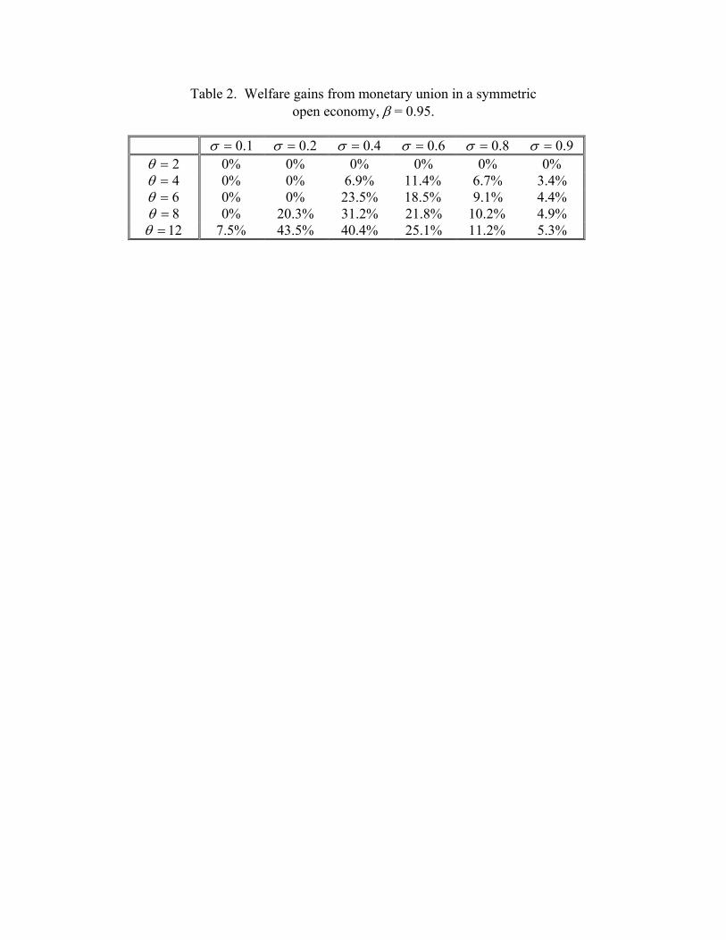
Table 2. Welfare gains from monetary union in a symmetric open economy, β = 0.95.

1.0=σ 2.0=σ 4.0=σ 6.0=σ 8.0=σ 9.0=σ

2=θ %0 %0 %0 %0 %0 %0 4=θ %0 %0 %9.6 %4.11 %7.6 %4.3 6=θ %0 %0 %5.23 %5.18 %1.9 %4.4 8=θ %0 %3.20 %2.31 %8.21 %2.10 %9.4

12=θ %5.7 %5.43 %4.40 %1.25 %2.11 %3.5

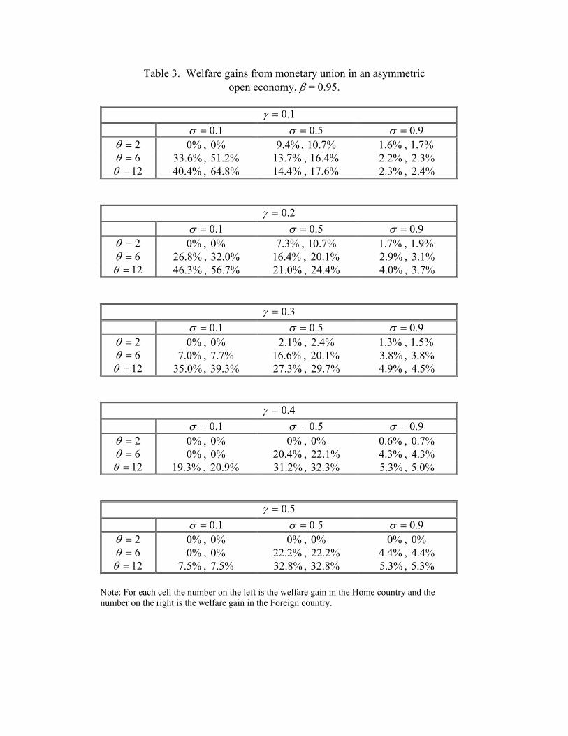
Table 3. Welfare gains from monetary union in an asymmetric open economy, β = 0.95.

1.0=γ

1.0=σ 5.0=σ 9.0=σ 2=θ %0 , 0 % %4.9 , 10 %7. %6.1 , 1 %7.6=θ %6.33 , 51 %2. %7.13 , 16 %4. %2.2 , 2 %3.

12=θ %4.40 , 64 %8. %4.14 , 17 %6. %3.2 , 2 %4. 2.0=γ

1.0=σ 5.0=σ 9.0=σ 2=θ %0 , 0 % %3.7 , 10 %7. %7.1 , 1 %9.6=θ %8.26 , 32 %0. %4.16 , %1.20 %9.2 , 3 %1.

12=θ %3.46 , 56 %7. %0.21 , 24 %4. %0.4 , 3 %7. 3.0=γ

1.0=σ 5.0=σ 9.0=σ 2=θ %0 , 0 % %1.2 , 2 %4. %3.1 , 1 %5.6=θ %0.7 , 7 %7. %6.16 , %1.20 %8.3 , 3 %8.

12=θ %0.35 , 39 %3. %3.27 , 29 %7. %9.4 , 4 %5. 4.0=γ

1.0=σ 5.0=σ 9.0=σ 2=θ %0 , 0 % %0 , 0 % %6.0 , 0 %7.6=θ %0 , 0 % %4.20 , 22 %1. %3.4 , 4 %3.

12=θ %3.19 , %9.20 %2.31 , 32 %3. %3.5 , 5 %0. 5.0=γ

1.0=σ 5.0=σ 9.0=σ 2=θ %0 , 0 % %0 , 0 % %0 , 0 %6=θ %0 , 0 % %2.22 , 22 %2. %4.4 , 4 %4.

12=θ %5.7 , 7 %5. %8.32 , 32 %8. %3.5 , 5 %3.

Note: For each cell the number on the left is the welfare gain in the Home country and the number on the right is the welfare gain in the Foreign country.

Figure 2: The Nash-Ramsey monetary policy in the closed vs. symmetricopen economy.

0.8

0.85

0.9

0.95

1

1.05

1.1

1.15

1.2

0 0.1 0.2 0.3 0.4 0.5 0.6 0.7 0.8 0.9 1

Sigma

Gro

ss ra

te o

f mon

ey g

row

th

Panel A: θ = 2, β = 0.95

Panel B: θ = (6, 12), β = 0.95

Closed economy and symmetric, open economy coincide at the Friedman rule

0.9

1

1.1

1.2

1.3

1.4

1.5

1.6

1.7

1.8

0 0.1 0.2 0.3 0.4 0.5 0.6 0.7 0.8 0.9 1

Sigma

Gro

ss ra

te o

f mon

ey g

row

th

Closed economy

Open economy, θ = 6

Open economy, θ = 12

dma6g

Figure 4. Pareto improving cooperative outcomes in the symmetric open economy.

dma6g

Figure 5. Pareto improving cooperative outcomes in the asymmetric open economy.