optimal matching distances between categorical sequences ...€¦ · optimal matching distances...
TRANSCRIPT
St. Cloud State UniversitytheRepository at St. Cloud State
Culminating Projects in Applied Statistics Department of Mathematics and Statistics
12-2013
Optimal Matching Distances between CategoricalSequences: Distortion and Inferences byPermutationJuan P. Zuluaga
Follow this and additional works at: http://repository.stcloudstate.edu/stat_etds
Part of the Applied Statistics Commons
This Thesis is brought to you for free and open access by the Department of Mathematics and Statistics at theRepository at St. Cloud State. It has beenaccepted for inclusion in Culminating Projects in Applied Statistics by an authorized administrator of theRepository at St. Cloud State. For moreinformation, please contact [email protected].
Recommended CitationZuluaga, Juan P., "Optimal Matching Distances between Categorical Sequences: Distortion and Inferences by Permutation" (2013).Culminating Projects in Applied Statistics. Paper 8.
OPTIMAL MATCHING DISTANCES BETWEEN CATEGORICAL
SEQUENCES: DISTORTION AND INFERENCES BY PERMUTATION
by
Juan P. Zuluaga
B.A. Universidad de los Andes, Colombia, 1995
A Thesis
Submitted to the Graduate Faculty
of
St. Cloud State University
in Partial Fulfillment of the Requirements
for the Degree
Master of Science
St. Cloud, Minnesota
December, 2013

This thesis submitted by Juan P. Zuluaga in partial fulfillment of therequirements for the Degree of Master of Science at St. Cloud State University ishereby approved by the final evaluation committee.
Chairperson
DeanSchool of Graduate Studies
OPTIMAL MATCHING DISTANCES BETWEEN CATEGORICALSEQUENCES: DISTORTION AND INFERENCES BY PERMUTATION
Juan P. Zuluaga
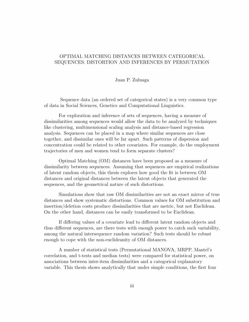
Sequence data (an ordered set of categorical states) is a very common typeof data in Social Sciences, Genetics and Computational Linguistics.
For exploration and inference of sets of sequences, having a measure ofdissimilarities among sequences would allow the data to be analyzed by techniqueslike clustering, multimensional scaling analysis and distance-based regressionanalysis. Sequences can be placed in a map where similar sequences are closetogether, and dissimilar ones will be far apart. Such patterns of dispersion andconcentration could be related to other covariates. For example, do the employmenttrajectories of men and women tend to form separate clusters?
Optimal Matching (OM) distances have been proposed as a measure ofdissimilarity between sequences. Assuming that sequences are empirical realizationsof latent random objects, this thesis explores how good the fit is between OMdistances and original distances between the latent objects that generated thesequences, and the geometrical nature of such distortions.
Simulations show that raw OM dissimilarities are not an exact mirror of truedistances and show systematic distortions. Common values for OM substitution andinsertion/deletion costs produce dissimilarities that are metric, but not Euclidean.On the other hand, distances can be easily transformed to be Euclidean.
If differing values of a covariate lead to different latent random objects andthus different sequences, are there tests with enough power to catch such variability,among the natural intersequence random variation? Such tests should be robustenough to cope with the non-euclideanity of OM distances.
A number of statistical tests (Permutational MANOVA, MRPP, Mantel’scorrelation, and t-tests and median tests) were compared for statistical power, onassociations between inter-item dissimilarities and a categorical explanatoryvariable. This thesis shows analytically that under simple conditions, the first four
iii

tests are mathematically equivalent. Simulations confirmed that tests had the samepower. Tests are less powerful with longer sequences.
Month Year Approved by Research Committee:
Hui Xu Chairperson
iv

ACKNOWLEDGMENTS
I would like to thank a number of people who provided essential support for
the completion of this thesis: my advisor, Dr. Hui Xu, for his encouragement,
interest, and patience; the members of my thesis committee; the faculty of the
Statistics department in general; the Business Computing Research Laboratory
(BCRL); the Office of Research and Sponsored Programs; Dr. Robert Johnson at
Precollege Programs; the library of St. Cloud State University, especially
Inter-Library Loan.
To Tina, thank you for your love and support all these years.
v

To my father.
vi
TABLE OF CONTENTS
Page
List of Figures . . . . . . . . . . . . . . . . . . . . . . . . . . . . . . . . . ix
Chapter
I. Introduction . . . . . . . . . . . . . . . . . . . . . . . . . . . . . 1
Substantive motivation . . . . . . . . . . . . . . . . . . . . 1
Dissimilarity among sequences by Optimal Matching . 4
From exploration to explanation . . . . . . . . . . . . . 7
Clustering . . . . . . . . . . . . . . . . . . . . . . . . . . . . 7
Extracting Dimensions . . . . . . . . . . . . . . . . . . . . . 8
Permutational Approaches on Raw Dissimilarities . . . . . . 10
Research questions . . . . . . . . . . . . . . . . . . . . . . . 11
II. Exploring intersequence distances . . . . . . . . . . . . . . 12
Generating sequences . . . . . . . . . . . . . . . . . . . . . 12
Does OM represent true dissimilarities? . . . . . . . . . 15
How Much Distortion? . . . . . . . . . . . . . . . . . . . . . 21
Distortion Affected by Sequence Length and OM Costs . . . 23
Geometric properties of distances . . . . . . . . . . . . . 28
OM as Metric . . . . . . . . . . . . . . . . . . . . . . . . . . 28
OM as City Block Distance . . . . . . . . . . . . . . . . . . . 30
Euclideanity of OM and Euclidean Transformations . . . . . 31
vii

Chapter Page
Distribution of inter-sequence distances . . . . . . . . . 36
Distribution of True Inter-Triple and OM Distances . . . . . 36
Multinormal Baseline . . . . . . . . . . . . . . . . . . . . . . 39
III. Statistical tests for inference . . . . . . . . . . . . . . . . . 42
MANOVA on Principal Coordinates . . . . . . . . . . . . . . 43
Mantel Test . . . . . . . . . . . . . . . . . . . . . . . . . . . 43
Permutational MANOVA . . . . . . . . . . . . . . . . . . . . 49
MRPP . . . . . . . . . . . . . . . . . . . . . . . . . . . . . . 52
IV. A comparison of power . . . . . . . . . . . . . . . . . . . . . . 55
General strategy . . . . . . . . . . . . . . . . . . . . . . . . 55
Making Use of Parametric Information . . . . . . . . . . . . 56
Simulation . . . . . . . . . . . . . . . . . . . . . . . . . . . . . 58
Changing Start Parameter, Fixing Rate . . . . . . . . . . . . 59
Changing Rate (Keeping Start Fixed) . . . . . . . . . . . . . 61
The Effect of Length of Sequence in Power of Tests . . . . . 63
V. Analytical identity between Mantel and Permanova . . 67
VI. Conclusions . . . . . . . . . . . . . . . . . . . . . . . . . . . . . . 69
Future work . . . . . . . . . . . . . . . . . . . . . . . . . . . 70
References . . . . . . . . . . . . . . . . . . . . . . . . . . . . . . . . . . . . 71
Appendices
A. Parallelizing the code . . . . . . . . . . . . . . . . . . . . . . 77
B. Checking for correctness of Distortion measure . . . . . 80
C. R source code . . . . . . . . . . . . . . . . . . . . . . . . . . . 85
viii
LIST OF FIGURES
Figure Page
1. Education/Job trajectories of Northern Irish young adults . . . . . . 2
2. MDS plot of 10 sequences . . . . . . . . . . . . . . . . . . . . . . . . 9
3. 5 sequences from a population, 5 from other. . . . . . . . . . . . . . . 16
4. Fit between OM distances (below) and true inter-triple distances (above). 18
5. Shepard plot of true distances Vs. OM distances . . . . . . . . . . . . 19
6. Shepard plot of true distances Vs. Square Root of OM distances . . . 21
7. Distortion, by length of sequence . . . . . . . . . . . . . . . . . . . . 24
8. Correlation by length of sequence . . . . . . . . . . . . . . . . . . . . 25
9. Distortion, changing indel cost, fixed subst=2 . . . . . . . . . . . . . 27
10. Proportion of Euclidean distance matrices . . . . . . . . . . . . . . . 33
11. Comparing MDS and OM distortions vs true inter-triple distances . . 35
12. Lengths of true inter-triple distances . . . . . . . . . . . . . . . . . . 37
13. Lengths of OM distances . . . . . . . . . . . . . . . . . . . . . . . . . 38
14. Lengths of MDS solution to OM distances . . . . . . . . . . . . . . . 39
15. Lengths of inter-item distances, multinormal distribution . . . . . . . 40
16. Power of tests, by values of Start parameter (Rate fixed) . . . . . . . 60
17. Power of tests, by values of Rate parameter (Start fixed) . . . . . . . 62
18. Power of tests, by length of sequences (Start and Rate fixed) . . . . . 64
19. Power by Seq Length, keeping triples truncated . . . . . . . . . . . . 66
ix

Chapter I
INTRODUCTION
SUBSTANTIVE MOTIVATION
The statistical examination in this thesis was motivated by a body of
sociological and economic research on biographical trajectories. As an example of
such empirical research work, McVicar & Anyadike-Danes (2002) tracked 712 young
people in Northern Ireland for six years (72 months). During every month the
person could be enrolled in school (of various kinds), in college, employed or jobless.
Their educational and work longitudinal trajectories were to be explained in
terms of individual demographic characteristics.
For example, see raw data on the trajectories for the first six months for the
first 10 people in the McVicar & Anyadike-Danes (2002) dataset mentioned above:
in Figure 1, every horizontal row represent the trajectories of the first 10 people (in
the dataset mentioned above); from left to right, colored tiles represent the state the
person was for some of the 72 months1 . (These plots and computations are made
using the TraMineR package (Gabadinho, Ritschard, Muller, & Studer, 2011) from
R (R Core Team, 2012)).
1In this dataset that comes from the educational system in Northern Ireland, young people stillcompleting classes within their compulsory education are labeled as “In School” ; students may optto enroll in some years of Further Education (equivalent to the last years of High School in theUS); the equivalent to US College education would be Higher Education. Training is a governmentsupported program of apprenticeships.
1

2
10 s
eq. (
n=71
2)
Sep.93 Sep.94 Sep.95 Sep.96 Sep.97 Sep.98
12
34
56
78
910
EmployedFurther Education
Higher EducationJobless
In SchoolTraining
Figure 1
Education/Job trajectories of Northern Irish young adults

3
A trajectory is defined as an ordered (sequence AB is not the same as
sequence BA) longitudinal set of categorical states in which the states are mutually
exclusive (a person cannot be in both state A and B at the same time). (In this
document I use trajectories and sequences as equivalents. Since I have in mind
biographical trajectories I will be referring to individuals or subjects to the entity
that goes through the states; but they should be thought of as any generic entity or
item).
Traditional statistical methods have been employed to answer some questions
about this type of data. Survival analysis (aka Event History Analysis in the Social
Science literature) (Klein & Moeschberger, 2007; Yamaguchi, 1991; Blossfeld &
Rohwer, 2002) can be used to explain the length of time to an event. Some
hierarchical or repeated-measures models for categorical outcomes in a generalized
linear frame have also been used (Ware & Lipsitz, 1988; Diggle, Liang, & Zeger,
1994). However, these traditional approaches have two major problems: they are
based on assumptions about the data generating process (assumptions that may be
unjustified), and their description is complex and even cumbersome due to their fine
granularity (as they model specific stays or transitions through time).
An alternative approach, free of assumptions about the probability
mechanism that generates the sequences, begins by condensing the information from
each sequence by an indicator such as Elzinga’s measure of complexity or turbulence
(Elzinga, 2010). This indicator can be considered as the dependent variable in a
regression, with individual level covariates as explanatory variables, to answer
questions like “did people born before 1970 have more turbulent trajectories?”.
Instead of directly analyzing instances of a random quantity (like observing a
4
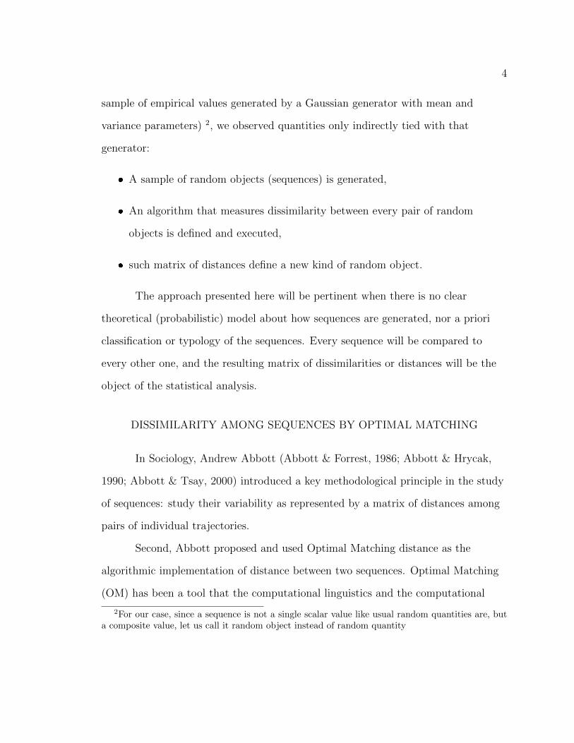
sample of empirical values generated by a Gaussian generator with mean and
variance parameters) 2, we observed quantities only indirectly tied with that
generator:
� A sample of random objects (sequences) is generated,
� An algorithm that measures dissimilarity between every pair of random
objects is defined and executed,
� such matrix of distances define a new kind of random object.
The approach presented here will be pertinent when there is no clear
theoretical (probabilistic) model about how sequences are generated, nor a priori
classification or typology of the sequences. Every sequence will be compared to
every other one, and the resulting matrix of dissimilarities or distances will be the
object of the statistical analysis.
DISSIMILARITY AMONG SEQUENCES BY OPTIMAL MATCHING
In Sociology, Andrew Abbott (Abbott & Forrest, 1986; Abbott & Hrycak,
1990; Abbott & Tsay, 2000) introduced a key methodological principle in the study
of sequences: study their variability as represented by a matrix of distances among
pairs of individual trajectories.
Second, Abbott proposed and used Optimal Matching distance as the
algorithmic implementation of distance between two sequences. Optimal Matching
(OM) has been a tool that the computational linguistics and the computational
2For our case, since a sequence is not a single scalar value like usual random quantities are, buta composite value, let us call it random object instead of random quantity
5
biology community have developed to compare strings of characters or genetic
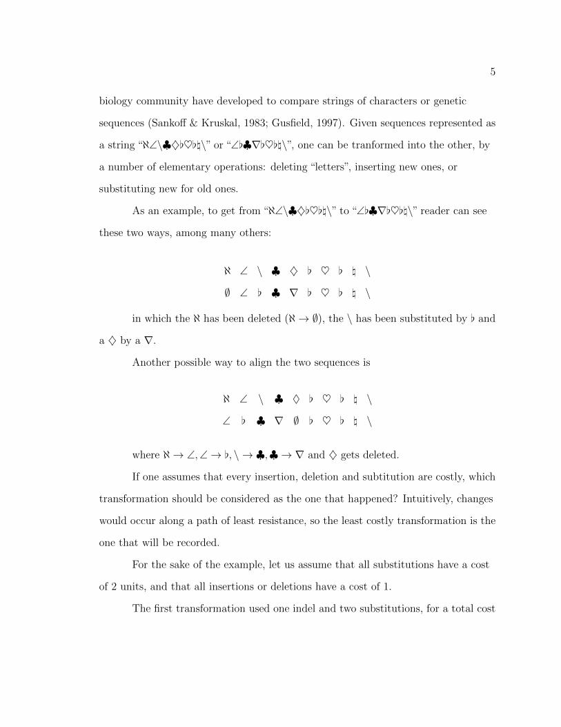
sequences (Sankoff & Kruskal, 1983; Gusfield, 1997). Given sequences represented as
a string “ℵ∠\♣♦[♥[\\” or “∠[♣∇[♥[\\”, one can be tranformed into the other, by
a number of elementary operations: deleting “letters”, inserting new ones, or
substituting new for old ones.
As an example, to get from “ℵ∠\♣♦[♥[\\” to “∠[♣∇[♥[\\” reader can see
these two ways, among many others:
ℵ ∠ \ ♣ ♦ [ ♥ [ \ \
∅ ∠ [ ♣ ∇ [ ♥ [ \ \
in which the ℵ has been deleted (ℵ → ∅), the \ has been substituted by [ and
a ♦ by a ∇.
Another possible way to align the two sequences is
ℵ ∠ \ ♣ ♦ [ ♥ [ \ \
∠ [ ♣ ∇ ∅ [ ♥ [ \ \
where ℵ → ∠,∠→ [, \ → ♣,♣ → ∇ and ♦ gets deleted.
If one assumes that every insertion, deletion and subtitution are costly, which
transformation should be considered as the one that happened? Intuitively, changes
would occur along a path of least resistance, so the least costly transformation is the
one that will be recorded.
For the sake of the example, let us assume that all substitutions have a cost
of 2 units, and that all insertions or deletions have a cost of 1.
The first transformation used one indel and two substitutions, for a total cost

6
of 1 + 2 + 2 = 5, while the second trasformation used one indel and four
substitutions, for a total cost of 9. If 5 is really the least costly transformation, we
can assign that 5 as a dissimilary measure.
For example, let us calculate a distance matrix with Optimal Matching for
the first 10 people in the mvad dataset used before3:
[,1] [,2] [,3] [,4] [,5] [,6] [,7] [,8] [,9] [,10][1,] 0 140 116 108 140 64 60 44 38 48[2,] 140 0 72 140 22 140 80 96 140 140[3,] 116 72 0 68 90 72 60 76 78 116[4,] 108 140 68 0 140 46 112 112 70 94[5,] 140 22 90 140 0 140 90 96 140 140[6,] 64 140 72 46 140 0 68 68 26 66[7,] 60 80 60 112 90 68 0 16 60 60[8,] 44 96 76 112 96 68 16 0 44 48[9,] 38 140 78 70 140 26 60 44 0 48[10,] 48 140 116 94 140 66 60 48 48 0
See how the distance between sequence 7 and sequence 8 is quite small, while
the distance between sequence 1 and 2 is large. Distance numbers do agree with the
intuitive sense derived from observing Figure 1.
At this point, the reader will certainly guess that the distance measure
depends on a prior matrix of subtitution and insertion–deletion costs. Such prior
values, where do they come from?
In the empirical tradition of sociological studies, researchers can make a
guess at costs based on substantive knowledge, for instance, by using information
about ordination of states, or they can assume explicit ignorance, by making all
substitution costs have the same value.
3Distance to be calculated with a substitution matrix set at equal costs (2) for all, and aninsertion–deletion (indel) cost set at 1.

7
Choices of prior costs has been subject to strong criticism and debate
(Levine, 2000; Wu, 2000; Abbott, 2000) and has opened a number of developments,
such as refinements for Optimal Matching distance measures (Lesnard, 2010;
Gauthier, Widmer, Bucher, & Notredame, 2009).
FROM EXPLORATION TO EXPLANATION
Clustering
The matrix of inter-sequence distances can be subject to clustering
procedures 4, allowing the allocation of individual trajectories into a few
archetypical trajectories. Such multinomial outcome can be explained by subject
attributes by fitting a multinomial logistic model. As an example, if 200 academic
trajectories of college students could be classed into 5 groups, could we use the race
or income of each student as a predictor of its trajectory being of a type 3 instead of
a type 1? McVicar & Anyadike-Danes (2002) is a good example of such approach.
However, going from similarity matrices to a mapping of clusters loses
information, since within each cluster all trajectories are assumed to be the same.
Instead, alternative approches use the pairwise distances explicitly as a measure of
variability (or discrepancy as Studer, Ritschard, Gabadinho, & Muller (2011) call it)
to be explained by covariates.
4Deciding which clustering procedure makes sense, among the many available is not a trivialproblem (Kaufman & Rousseeuw, 1990)
8
Extracting Dimensions
A set of coordinates in a lower dimensional space can be found that
approximates the raw matrix of inter-item distances, by means of Multidimensional
Scaling Algorithms (either non-metric or metric – Principal Coordinates being a
classical metric kind).
While we can assume that reducing raw distances to a lower space causes
some information loss, a clear advantage is the ability to work with much less
parameters.
Coordinates in a lower dimensional space can be used to make a 2 or 3
dimensional plot of items, and perhaps adding colors or shapes to items by their
attributes.
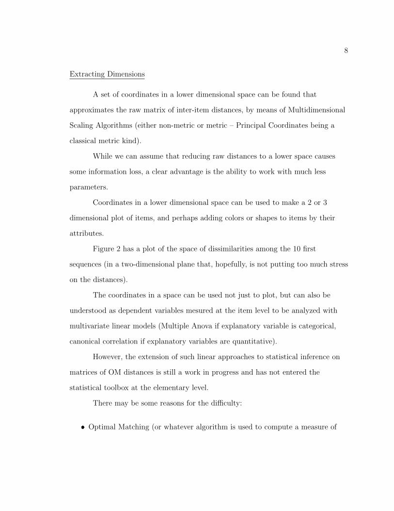
Figure 2 has a plot of the space of dissimilarities among the 10 first
sequences (in a two-dimensional plane that, hopefully, is not putting too much stress
on the distances).
The coordinates in a space can be used not just to plot, but can also be
understood as dependent variables mesured at the item level to be analyzed with
multivariate linear models (Multiple Anova if explanatory variable is categorical,
canonical correlation if explanatory variables are quantitative).
However, the extension of such linear approaches to statistical inference on
matrices of OM distances is still a work in progress and has not entered the
statistical toolbox at the elementary level.
There may be some reasons for the difficulty:
� Optimal Matching (or whatever algorithm is used to compute a measure of

9
●
●
●
●
●
●
●
●
●
●
−100 −50 0 50
−60
−40
−20
020
40
Nonmetric MDS on 10 sequences
Coordinate 1
Coo
rdin
ate
2
1
2
3
4
5
6
7
8
9
10
Figure 2
MDS plot of 10 sequences

10
dissimilarity between sequences) may be a biased representation of the
dissimilarities among the true entities behind the sequence.
� the raw dissimilarities among items may not be metric or Euclidean at all,
some mathematical operations with them may not be appropriate, and some
conclusions may be suspicious.
� the distributions of the items (or a monotone transformation of them) may not
follow a multivariate normal shape (the most tractable multivariate
distribution) and MANOVA may not be robust enough against violations of
the assumptions.
Permutational Approaches on Raw Dissimilarities
A way to bypass the concern with the geometric and distributional properties
of inter-item distances for statistical inference is by simulation, specifically
permutational strategies.
In the permutational strategy a Null Hypothesis is proposed and
operationalized as a baseline, as the theoretically possible set of variations by
permutation of the original matrix of distances.
Furthermore, as in Permutational MANOVA (Anderson, 2001), a measure of
variability and discrepancy among items is operationalizaed, to be partitioned by
covariates (perhaps in a regression tree).
A number of permutational approaches have been proposed by applied
researchers in dissimilar fields like Spatial Statistics (Mantel, 1967; Mielke & Berry,
2001), Psychometrics (Hubert & Schultz, 1976), and Ecology (Manly, 1997;

11
Anderson, 2001). It seems worthwhile to clarify the differences and commonalities
among these various approaches (Reiss et al., 2010).
RESEARCH QUESTIONS
First, I will describe the sequence generator to be used. Of the very many
possible generators, this one was chosen because it was used by Studer et al. (2011).
Second, I study properties of such Optimal Matching distances, particularly
what I call representational, geometric and distributional characteristics.
These two items will be contained in chapter II of this thesis.
Iin the third chapter I will describe and compare the power of some
statistical methods for inference on Optimal Matching distance matrices: Mantel’s
test, permutational MANOVA (Permanova), Multiresponse permutational
procedure (MRPP) and a test that uses Principal Coordinates (PCoA) from the
matrix of distances for simple one way analysis. These tests make almost no
assumptions about the process that generated the sequences. Some additional tests,
that “cheat” by incorporate some knowledge about the sequence generation, will be
run and their power compared.
In the fourth chapter I will explain the similarities between Mantel’s test,
PerManova and MRPP, by studying their algebraic formulation.
Chapter II
EXPLORING INTERSEQUENCE DISTANCES
GENERATING SEQUENCES
Many sequence generators could be imagined; I chose the generators in
Studer et al. (2011) for being a key paper in the literature. A good alternative could
be the ones described in Wilson (2006).
Studer et al. (2011), in the simulations they run, present three extremely
simple mechanisms to generate sequences. Their simplicity consists in requiring few
parameters (unlike, say, Markov chains, that would require n(n− 1) parameters to
describe a transition matrix among n states). The sequences are both simple but
still interesting.
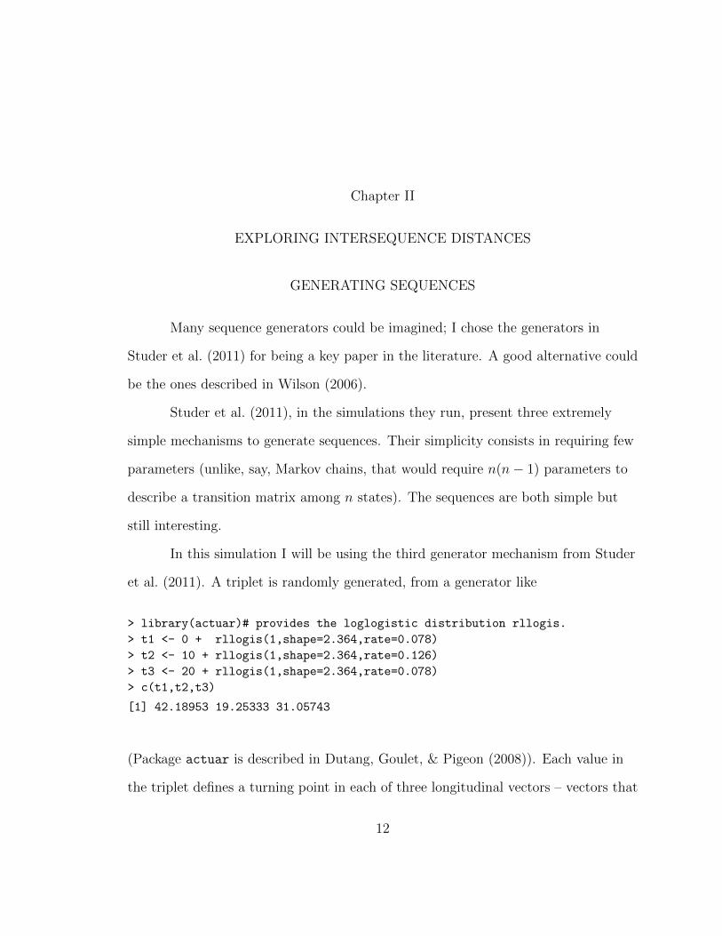
In this simulation I will be using the third generator mechanism from Studer
et al. (2011). A triplet is randomly generated, from a generator like
> library(actuar)# provides the loglogistic distribution rllogis.
> t1 <- 0 + rllogis(1,shape=2.364,rate=0.078)
> t2 <- 10 + rllogis(1,shape=2.364,rate=0.126)
> t3 <- 20 + rllogis(1,shape=2.364,rate=0.078)
> c(t1,t2,t3)
[1] 42.18953 19.25333 31.05743
(Package actuar is described in Dutang, Goulet, & Pigeon (2008)). Each value in
the triplet defines a turning point in each of three longitudinal vectors – vectors that
12
13
correspond to columns S1, S2, S3 as seen in computer output; see how they
usually start (at row 1) being 0, and then turn to 1 at a row that depends on the
value of t1, t2, t3. We can think of every row representing a point in time; at
each point there is a triple of three binary states. There can be 8 (23) possible triples
(000, 001, ..., 111) that can be finally represented, as an example, by their decimal
equivalent. This final digit (“0” to “7”) represents a category, not a numerically
valued dimension (state “7” is not seven times whatever state “1” is, it just
represents a state 111 versus state 001). (Time sequence goes from top to bottom.
Hidden presequences are S1, S2, S3, final categorical sequence is s.final.)

14
S1 S2 S3 s.final1 0 0 0 02 0 0 0 03 0 0 0 04 0 0 0 05 0 0 0 06 0 0 0 07 0 0 0 08 0 0 0 09 0 0 0 010 0 0 0 011 0 0 0 012 0 0 0 013 0 0 0 014 0 0 0 015 0 0 0 016 0 0 0 017 0 0 0 018 0 0 0 019 0 0 0 020 0 1 0 221 0 1 0 222 0 1 0 223 0 1 0 224 0 1 0 225 0 1 0 226 0 1 0 227 0 1 0 228 0 1 0 229 0 1 0 230 0 1 0 231 0 1 0 232 0 1 1 333 0 1 1 334 0 1 1 335 0 1 1 336 0 1 1 337 0 1 1 338 0 1 1 339 0 1 1 340 0 1 1 3
Using the same parameters for shape and intensity that were used by Studer
et al. (shape=2.364, intensity=0.078, start={0,10,20}), results in a last column that
is the combined outcome of the three preliminary sequences generated from three
log-logistic points of transition.
15
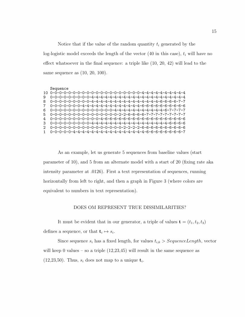
Notice that if the value of the random quantity ti generated by the
log-logistic model exceeds the length of the vector (40 in this case), ti will have no
effect whatsoever in the final sequence: a triple like (10, 20, 42) will lead to the
same sequence as (10, 20, 100).
Sequence10 0-0-0-0-0-0-0-0-0-0-0-0-0-0-0-0-0-0-0-0-4-4-4-4-4-4-4-4-4-49 0-0-0-0-0-0-0-0-0-4-4-4-4-4-4-4-4-4-4-4-4-4-4-4-4-4-4-4-4-48 0-0-0-0-0-0-0-0-0-4-4-4-4-4-4-4-4-4-4-4-4-4-4-4-6-6-6-6-7-77 0-0-0-0-0-0-0-4-4-4-4-4-4-4-4-4-4-4-4-4-6-6-6-6-6-6-6-6-6-66 0-0-0-0-0-0-0-0-0-0-0-0-0-0-4-4-4-4-4-4-4-4-4-4-4-6-7-7-7-75 0-0-0-0-0-0-0-0-0-0-0-0-0-0-0-2-2-6-6-6-6-7-7-7-7-7-7-7-7-74 0-0-0-0-0-0-0-0-0-0-0-4-6-6-6-6-6-6-6-6-6-6-6-6-6-6-6-6-6-63 0-0-0-0-0-0-0-0-0-4-4-4-4-4-4-4-4-4-4-4-4-4-4-4-4-4-6-6-6-62 0-0-0-0-0-0-0-0-0-0-0-0-0-0-0-0-2-2-2-2-6-6-6-6-6-6-6-6-6-61 0-0-0-0-0-4-4-4-4-4-4-4-4-4-4-4-4-4-4-4-4-6-6-6-6-6-6-6-6-7
As an example, let us generate 5 sequences from baseline values (start
parameter of 10), and 5 from an alternate model with a start of 20 (fixing rate aka
intensity parameter at .0126). First a text representation of sequences, running
horizontally from left to right, and then a graph in Figure 3 (where colors are
equivalent to numbers in text representation).
DOES OM REPRESENT TRUE DISSIMILARITIES?
It must be evident that in our generator, a triple of values t = (t1, t2, t3)
defines a sequence, or that ti 7→ si.
Since sequence si has a fixed length, for values ti,k > SequenceLength, vector
will keep 0 values – so a triple (12,23,45) will result in the same sequence as
(12,23,50). Thus, si does not map to a unique ti.

16
10 s
eq. (
n=10
)
T1 T4 T7 T10 T13 T16 T19 T22 T25 T28
12
34
56
78
910
02
46
7
Figure 3
5 sequences from a population, 5 from other.
17
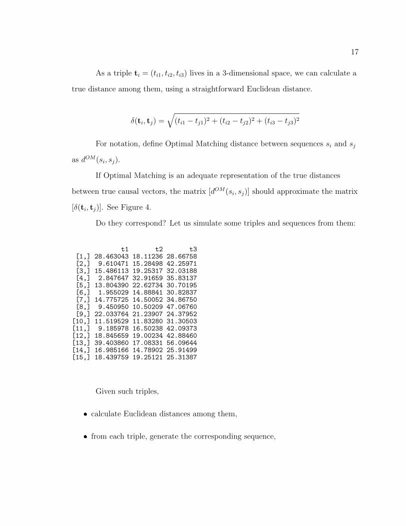
As a triple ti = (ti1, ti2, ti3) lives in a 3-dimensional space, we can calculate a
true distance among them, using a straightforward Euclidean distance.
δ(ti, tj) =√
(ti1 − tj1)2 + (ti2 − tj2)2 + (ti3 − tj3)2
For notation, define Optimal Matching distance between sequences si and sj
as dOM(si, sj).
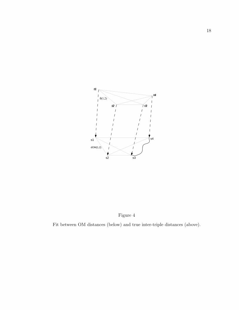
If Optimal Matching is an adequate representation of the true distances
between true causal vectors, the matrix [dOM(si, sj)] should approximate the matrix
[δ(ti, tj)]. See Figure 4.
Do they correspond? Let us simulate some triples and sequences from them:
t1 t2 t3[1,] 28.463043 18.11236 28.66758[2,] 9.610471 15.28498 42.25971[3,] 15.486113 19.25317 32.03188[4,] 2.847647 32.91659 35.83137[5,] 13.804390 22.62734 30.70195[6,] 1.955029 14.88841 30.82837[7,] 14.775725 14.50052 34.86750[8,] 9.450950 10.50209 47.06760[9,] 22.033764 21.23907 24.37952[10,] 11.519529 11.83280 31.30503[11,] 9.185978 16.50238 42.09373[12,] 18.845659 19.00234 42.88460[13,] 39.403860 17.08331 56.09644[14,] 16.985166 14.78902 25.91499[15,] 18.439759 19.25121 25.31387
Given such triples,
� calculate Euclidean distances among them,
� from each triple, generate the corresponding sequence,
18
t1
t2
t4
t3
s1
s2 s3
s4
dOM(1,2)
Figure 4
Fit between OM distances (below) and true inter-triple distances (above).
19
●
●
●
●
●
●
●
●
●
●
●
●●
●
●
●
●●
●
●
●
●
●
●
●
●
●
●
●
●
●
●
●
●
●
●
●
●●
●
●
●
●
●●
●
●
●
●●
●●
●
●
●
●
●
●
●●
●
●
●
●
●
●
●
●
●
●
●
●
●
●
●
●
●
●
●
●
●
●
●
●
●
●
●●
●
●
●
●
●
●
●
●
●
●
●
●
●
●
●●
●
0 10 20 30 40
020
4060
Euclidean distance among triples delta(ti,tj)
Opt
imal
Mat
chin
g di
stan
ce a
mon
g se
quen
ces
d(si
,sj)
Figure 5
Shepard plot of true distances Vs. OM distances
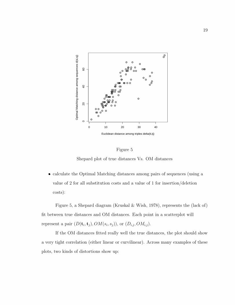
� calculate the Optimal Matching distances among pairs of sequences (using a
value of 2 for all substitution costs and a value of 1 for insertion/deletion
costs):
Figure 5, a Shepard diagram (Kruskal & Wish, 1978), represents the (lack of)
fit between true distances and OM distances. Each point in a scatterplot will
represent a pair (D(ti, tj), OM(si, sj)), or (Di,j, OMi,j).
If the OM distances fitted really well the true distances, the plot should show
a very tight correlation (either linear or curvilinear). Across many examples of these
plots, two kinds of distortions show up:

20
� a region of points located to the right of the plot, with high true Euclidean
distances, but corresponding dOM not high. They are due to cases where one
or more tik components of (ti1, ti2, ti3) were considerably greater than 40; the
resulting sequence si, however, could not be very distinct from other sequences
where the outlying tik ≈ 40. So while in the Euclidean space such triple was
far apart from others, in the OM pseudo-space1 the corresponding sequence
was not an outlier.
� when, by chance, such outlier triples are generated, and the points are better
distributed towards the right side of the graph, it can be seen that the higher
the true Euclidean distance, the higher the variance in OM distances. Points
are distributed in the shape of a folding fan. The distortion grows with the
magnitude of the distance, as it happens when a measure is a sum of other
measures with weak or no correlation among them, its total variance being
close to the sum of the variances of the components.
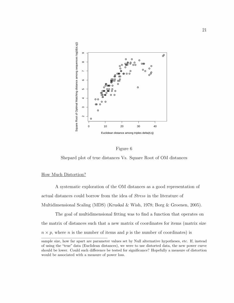
The plot of distortions suggests that some transformations of the original
data could help in this situation. For instance, what if the squared distance of OM
distances was used instead? Figure 6 shows that the graph is a bit more tight. This
opens the consideration of appropriate transformations, in coming sections.
A visual exploration of such distortions of representation is not enough. We
would need a measure of such distortion – and even more interesting, a measure of
how much such distortion affects the power of statistical tests2
1“Pseudo-space” because, at this point of the presentation, it is not clear if OM define a Euclideanspace.
2For now, only as a footnote, an approach could be like this: consider that the power of anstatistic is a function of the data employed and of other nuisance factors that affect the power:
21
●
●
●
●
●
●
●
●
●
●
●
●●
●
●
●
●●
●
●
●
●
●
●
●
●
●
●
●
●
●
●
●
●
●
●
●
●●
●
●
●
●
●●
●
●
●
●●
●●
●
●
●
●
●
●
●●
●
●
●
●
●
●
●
●
●
●
●
●
●
●
●
●
●
●
●
●
●
●
●
●
●
●
●●
●
●
●
●
●
●
●
●
●
●
●
●
●
●
●●
●
0 10 20 30 40
23
45
67
89
Euclidean distance among triples delta(ti,tj)
Squ
are
Roo
t of O
ptim
al M
atch
ing
dist
ance
am
ong
sequ
ence
s lo
g(d(
si,s
j))
Figure 6
Shepard plot of true distances Vs. Square Root of OM distances
How Much Distortion?
A systematic exploration of the OM distances as a good representation of
actual distances could borrow from the idea of Stress in the literature of
Multidimensional Scaling (MDS) (Kruskal & Wish, 1978; Borg & Groenen, 2005).
The goal of multidimensional fitting was to find a function that operates on
the matrix of distances such that a new matrix of coordinates for items (matrix size
n× p, where n is the number of items and p is the number of coordinates) is
sample size, how far apart are parameter values set by Null alternative hypotheses, etc. If, insteadof using the “true” data (Euclidean distances), we were to use distorted data, the new power curveshould be lower. Could such difference be tested for significance? Hopefully a measure of distortionwould be associated with a measure of power loss.

22
obtained, with items that fit in a space of lower dimensions (p less than original p∗),
while still preserving most of the inter-item distances from the original data.
Solutions could be evaluated to minimize stress, calculated, for instance, as
Stress =
√∑[f(pij)− dij]2∑
d2ij,
where pij is the empirical distances among items i and j, f(pij) is the
function on such matrix of empirical distances, and dij is an Euclidean distance
among the same items as they get relocated in a space of lower dimensions (more
precisely, euclidean distance obtained from the new coordinates of the items).
In our case, however, we just want a measure of representational distortion
between the “true” (Euclidean) distances between the vector (triple) t of quantities
that define sequences, and OM distances obtained among such sequences.
Distortion =
√∑[OMij − δij]2∑
OM2ij
where OMij is the calculated OM distance between sequences originated
from triples i and j, and δij is the true euclidean distance between triples i and j.
Why∑OM2
ij in denominator instead of∑δ2ij? Since choosing different
indel/substitution costs changes the values in the OM distance matrix, a measure of
Distortion should control for the total magnitude of such changes (∑OM2
ij).∑δ2ij
on the other hand is fixed.
A Pearson correlation coefficient could also be used – in fact it receives the
special name Cophenetic Correlation coefficient in the classification literature, when
the question of interest is how well clustering groupings fit an original matrix of
23
dissimilarities; following Wikipedia’s article on Cophenetic correlation, formula
would be
c =
∑i<j(OMij −OM)(δij − δ)√
[∑
i<j(OMij −OM)2][∑
i<j(δij − δ)2]
where OM is the average OM distance, and δ is the average inter-triple true
distance. The formula normalizes for matrices with non-normalized cell values.
In R, the Distortion function and the cophenetic correlation could be written
as
> Distortion = function(m1,m2) {
+ m1.s = m1
+ m2.s = m2
+ Numerator = sum(as.vector(( m1.s - m2.s)^2))
+ Denominator=sum(as.vector(m1.s^2))
+ return(sqrt(Numerator/Denominator))
+
+ }
> CopheneticCorrel = function(m1,m2) {
+ return(cor(as.vector(m1),as.vector(m2)))
+ }
>
>
See the appendix for some checks on the validity of this computation of
Distortion.
Distortion Affected by Sequence Length and OM Costs
Length: Now we can examine how much Distortion is there between the
inter-triple distance matrix and the inter-sequence OM distance matrix – controlling
24
●●
●
●
●
●●
●
●●
●
●
●
●
●
●●
●●
●
●
●
●
●
●
●
●●
●
●
●
●●
●
●
●●●
●●●●
●
●●
●
●
●
●●●
●●
●
●
●
●
●
●
●
●
●
●
●
●
●
●
●
●
●
●
●
●
●
●
●
●
●●
●
●
●
●
●
●
●
●●
●
●
●
●
●
●
●
●
●●●
●
●
●●
●●
●●
●
●
●
●
●●●
●●
●
●
●
●
●
●
●
●
●●
●
●
●●
●
●
●
●
●
●
●
●
●
●
●
●
●
●●
●
●
●
●
●
●
●
●
●
●
●●
●●
●
●
●
●
●
●
●●
●
●●●●
●●
●
●●
●
●
●
●
●
●
●
●●●
●
●●
●
●
●
●
●
●
●
●
●
●
●●
●
●
●
●
●
●
●
●●
●
●
●
●
●●
●
●
●
●
●
●
●
●
●
●
●
●
●●
●●●
●
●●●●●
●
●
●
●
●●●
●
●
●
●●
●
●
●
●
●●●
●
●●
●●
●
●
●
●●
●●
●●
●●
●
●
●
●
●
●
●
●
●
●●●●●
●
●
●
●
●
●
●
●
●
●
●
●
●
●
●
●
●●
●
●●
●
●
●
●●
●
●●
●●
●
●
●
●
●
●
●
●
●
●
●
●
●
●
●
●●
●
●
●●
●●
●●●
●
●●
●
●
●
●
●
●●
●
●
●
●
●
●
●
●
●●●
●
●
●
●
●●●●
●●
●
●
●●
●
●
●
●
●
●
●●●
●●
●
●
●
●
●
●
●
●
●
●
●
●
●●
●●
●
●
●
●●
●
●
●
●
●
●
●
●
●
●
●
●
●
●
●●
●●
●
●
●●
●
●
●
●
●
●
●●
●
●
●●
●
●
●
●
●●
●
●●
●
●
●
●
●
●
●●●
●●●●●
●
●
●
●
●
●
●●
●●
●●
●
●
●
●
●●
●
●
●
●
●
●
●
●
●
●
●
●●
●●
●●
●
●
●
●
●
●
●
●
●
●
●
●
●
●●●●
●
●
●
●
●●
●
●●
●●●
●
●●
●●
●
●
●●
●
●
●●
●
●
●●
●
●
●
●
●
●
●
●
●
●
●
●
●
●●
●
●
●
●
●
●
●
●
●
●
●
●
●
●●
●
●
●
●●●
●●
●
●
●
●●●●
●
●
●
●●
●
●
●
●
●
●
●
●
●
●●●●
●
●
35 40 45 50 55
0.5
1.0
2.0
5.0
10.0
Sequence Length
Mea
sure
of D
isto
rtio
n
Figure 7
Distortion, by length of sequence
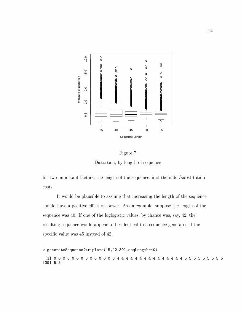
for two important factors, the length of the sequence, and the indel/substitution
costs.
It would be plausible to assume that increasing the length of the sequence
should have a positive effect on power. As an example, suppose the length of the
sequence was 40. If one of the loglogistic values, by chance was, say, 42, the
resulting sequence would appear to be identical to a sequence generated if the
specific value was 45 instead of 42.
> generateSequence(triple=c(15,42,30),seqLength=40)
[1] 0 0 0 0 0 0 0 0 0 0 0 0 0 0 4 4 4 4 4 4 4 4 4 4 4 4 4 4 4 5 5 5 5 5 5 5 5 5[39] 5 5

25
●●●●●●
●●
●
●●●●
●●
●
●● ●●
●
●
●●●
●
●
●
●●
●●●●●●
●●
●
●
●
●
●●●●●
●
●
●
●
●
●
●
●
●●●
●
●
●
●●
●
●
●●
●
●
●
●
●
●
●●
●
●●●●
●
●
●
●
●
35 40 45 50 55
0.0
0.2
0.4
0.6
0.8
1.0
Sequence Length
Mea
sure
of C
orre
latio
n
Figure 8
Correlation by length of sequence
26
> generateSequence(triple=c(15,45,30),seqLength=40)
[1] 0 0 0 0 0 0 0 0 0 0 0 0 0 0 4 4 4 4 4 4 4 4 4 4 4 4 4 4 4 5 5 5 5 5 5 5 5 5[39] 5 5
However, if the length of the sequence is, say, 50, if triple A contains a value
42, and triple B contains a value 45, the sequence derived from triple A could be
observed to be different that one from triple B.
> generateSequence(triple=c(15,42,30),seqLength=50)
[1] 0 0 0 0 0 0 0 0 0 0 0 0 0 0 4 4 4 4 4 4 4 4 4 4 4 4 4 4 4 5 5 5 5 5 5 5 5 5[39] 5 5 5 7 7 7 7 7 7 7 7 7
> generateSequence(triple=c(15,45,30),seqLength=50)
[1] 0 0 0 0 0 0 0 0 0 0 0 0 0 0 4 4 4 4 4 4 4 4 4 4 4 4 4 4 4 5 5 5 5 5 5 5 5 5[39] 5 5 5 5 5 5 7 7 7 7 7 7
Increasing the length of the sequence, by increasing the ability to
differentiate between triples, should increase the accuracy of the representation.
Figure 7 shows that Distortion slightly decreases with length of sequence
(higher Distortion means worse fit). Effect is even more clear in Figure 8, that uses
the (Cophenetic) correlation measure (lowest correlation means worse fit).
OM Costs: There have been debates in the sociological literature on OM
distances for the study of sequences, about how indel/substitution costs are, to a
certain extent, arbitrary, and what good rules of judgement to use (Levine, 2000;
Wu, 2000; Gauthier et al., 2009; Abbott & Tsay, 2000; Macindoe & Abbott, 2003;
Lesnard, 2010).
27
●●
●
●
●
●
●
●
●
●
●
●
●
●
●
●
●
●
●
●●●●
●
●
●
●●
●●●●●●
●
●●●●●
●
●●●●●
●
●●
●
●
●
●
●
●
●●●●●●
●
●●●●●
●
●
●
●●●●●●
●
●
●
●
●
●
●
●
●●●●
●●●●●●●
●
●●
●
●●
●●
●
●
●●●
●●
●
●●
●●
●
●
●
●
●●
●
●
●●●●●
●●●
●●
●●
●
●●●●
●●●●●
●
●●●●
●
●
●
●
●
●
●
●
●
●●
●●
●
●
●
●
●●
●●
●
●
●
●
●
●
●
●
●●
●
●
●
●●●●●●
●
●
●
●
●●
●
●
●●●
●
●
●●
●
●●
●●
●
●●
●
●
●
●
●
●
●
●
●
●
●
●●
●
●
●
●
●
●
●
●
●●
●
●
●
●●
●●●
●
●
●
●●
●
●
●
●
●
●
●●●●●●
●
●
●
●●●●
●
●
●
●
●●●●●●
●●
●
●
●
●
●
●
●
●
●
●
●●●
●●●
●
●
●
●
●
●●●
●
●●
●
●
●
●
●
●
●●●
●
●
●●
●
●
●
●●●
●
●●●
●
●●
●
●●●●
●
●
●
●●
●
●
●
●
●●
●
●
●
●
●
●
●●●
●●
●●●
●
●●
●●
●
●●●
●
●●
●●●
●
●
●
●
●
●●
●
●
●
●●●
●
●
●
●
●●
●●●●
●
●
●
●●
●●●●●
●
●
●●
●
●●
●
●●●●●
●
●
●
●
●●
●
●
●
●
●●
●
●
●
●●●●
●
●
●
●●
●
● ●
●
●
●
●
●
●
●
●
●
●●●●
●
●
●
●●
●
●●●●●
●
●●●●
●
●●
●
●●
●●
●●●●
●
●
●
●
●
●
●
●
●
●
●
●●●
●
●
●●●
●●●
●
●
●●
●
●
●●
●
●
●●
●●
●●
●●●
●●
●●●●
●
●●
●●
●●●
●
●
●●●
●●●
●
●
●
●
●●
●●
●
●●●
●
●●
●
●●●
●●
●
●
●
●
●
●
●
●
●
●
●
●●
●
●
●●●
●
●
●
●
●
●
●
●
●●
●●●
●
●●
●
●
●●
●
●●
●
●●●
●
●
●●●
●
● ●
●
●
●
●●●
●
●
●●
●
●
●●
●
●
●
●
●
●
●
●
●
●●●
●
●
●
●
●
●
●●
●
●
●
●●●
●
●
●●●
●
●●●●●●●
●●
●
●●●●
●
●●
●
●●
●
●●●●
●
●
●
●
●●●●
●
●●●
●
●●
●
●
●●●●
●
●
●
●●●
●●
●●
●
●
●●
●
●
●
●●●
●
●●
●●●
●
●
●
●●
●
●
●
●
●
●
●
●
●
●
●
●●●
●
●
●●●●●●●
●
●
●●
●
●
●●●
●
●●
●
●
●●
●
●
●
●●
●
●
●
●
●
●
●●
●●
●
●●
●
●
●
●
●●
●
●
●
●
●●●●●●
●
●
●●●●
●●
●
●
●●●●●
●
●●
●
●●●
●
●●●●
●
●●
●●●
●●●●
●
●●
●
●
●
●
●
●
●
●
●
●●
●
●
●●●
●
●●●
●
●●●
●
●
●●●
●
●
●
●
●●●●
●●
●●
●
●
●
●
●
●
●
●
●
●●●●●●
●
●
●
●●
●
●●
●
●
●
●
●●
●●
●
●
●
●●
●
●
●
●
●
●
●
●
●●
●
●
●
●
●●●●●●
●
●●
●
●●
●
●
●●●●●
●
0.25 0.75 1 1.25 1.75 2 2.25 2.75 3
0.5
1.0
2.0
5.0
20.0
50.0
200.
0
Cost of Insertion−Deletion
Mea
sure
of D
isto
rtio
n
Figure 9
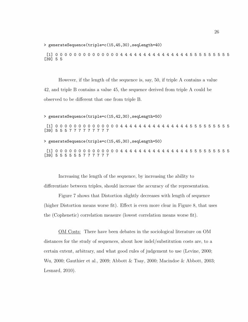
Distortion, changing indel cost, fixed subst=2
Here it is assumed that the matrix of substitutions is a constant 2 for all of
them (instead of some other plausible rules, like substitution costs same as
transition probabilities), and that the indel costs will range from 0.1 to 2.5.
See Figure 9 for a plot on the effect of varying the Insertion–Deletion cost
(and keeping substitution costs constant = 2) on the Distortion measure between
true distances (distances between original triplets) and OM distances among derived
sequences. Interestingly, indel costs don’t seem to affect Distortion – provided that
indel is greater than 1/2 of substitution costs.
28
GEOMETRIC PROPERTIES OF DISTANCES
Practicioners in Ecology (Legendre & Legendre, 1998) have developed many
measures of similarity and dissimilarity that are substantively relevant; however the
statistical and distributional consequences of so many alternative measures present a
challenge for the researcher that need to make inferences. As an example, analytical
definition of useful distributions for semimetric distances like the Bray-Curtis is an
open question.
In this particular sequence generator, distances among original triples are, of
course, embedded in a space of three dimensions.
Two questions are posed: first, do the OM distances between sequences
define a metric? Second, are they embedded in an euclidean space?
OM as Metric
An outcome matrix of distances is semimetric or pseudometric when it fulfills
three conditions (Legendre & Legendre, 1998):
minimum 0 : if sequence Si is the same as sequence Sj, then distance d(Si, Sj) = 0;
positiveness : if Si 6= Sj, d(i, j) > 0;
symmetry : d(i, j) = d(j, i).
Furthermore, a distance is metric when, in addition to the three previous
conditions, it fullfills the triangle inequality condition
d(Si, Sj) + d(Sj, Sk) ≥ d(Si, Sk).

29
The first condition needs no further explanation. If costs are defined for all
substitutions, insertions and deletions, there will always be a way to transform a
sequence into any other sequence, at a cost, so that cost will be defined. As for the
symmetry condition, it will be fulfilled if the matrix of substitution costs is
symmetric. In our generators, such matrix is assumed to be symmetric.
The triangle inequality condition can be easily proven true by considering
that, in order to transform sequence A to sequence C, it can be done by
transforming A to B, and then taking sequence B and transforming it to C. Such
transformation, via B, will have a cost d(B)(A,C) = d(A,B) + d(B,C), that defines
an upper bound for candidates for the true OM distance d(A,C).
d(A,B) + d(B,C) = d(B)(A,C) ≥ d(A,C)
Metricity of Transformed Distances Notice how, if distances were to be
squared, the triangle inequality is in doubt:
d2(B)(A,C) = (d(A,B) + d(B,C))2 = d2(A,B) + d2(B,C) + 2d(A,B)d(B,C)
Because of the 2d(A,B)d(B,C), we cannot prove that there is a d2(A,C)
such that d2(A,C) ≤ d2(A,B) + d2(B,C).
On the other hand, if we take the square root of distances, distances are still
metric. To prove that√d(AC) ≤
√d(AB) +
√d(BC) by contradiction, assume
that: √d(AC) >
√d(AB) +
√d(BC)
30
by squaring each side,
d(AC) > d(AB) + d(BC) + 2√d(AB)d(BC)
However we established before that true OM distance
d(AC) ≤ d(B)(AC) = d(AB) + d(BC), so we have arrived to a contradictory
statement.
A square root transformation is just a case of a more general kind of metric
preserving transformations. As an example, (Gower & Legendre, 1986, theorem 2,
page 7), that says “If D is metric then so are the matrices with elements (i) dij + c2,
(ii) d1/rij (where r ≥ 1) (iii) dij/(dij + c2) where c is any real constant”.
OM as City Block Distance
Suppose that the sequences of interest, to transform one to the other, are
SOCIOLOGY to PSYCHOLOGY.
Given the alphabet of states {S, O, C, I, L, G, Y, P, S, H, ∅}, (10 letters plus
an ∅ as an ”empty” state) and assuming that deleting X is just going from a state X
to a state ∅, and vice versa for an insertion, a transformation from one sequence to
another can be seen as a specific set of elementary exchanges of one state by other
state, among the possible (10 + 1)× 10/2 = 55 exchanges possible.
In this case, let us say that the transformation was very simple, exchanged
31
P/∅, Y/O,H/I, like this:
P S Y C H O L O G Y
∅ S O C I O L O G Y
Every one of those 55 possible exchanges define a dimension of distance. Of
all those 55 possible exchanges, only 3 were used.
In general, the cost of a transformation from sequences S to S ′ is a sum of
penalties incurred by a set of elementary exchange operations:
d(S, S ′) =n+1∑i=1
n+1∑j=i
w(ai, aj)ε(ai, aj)
Where i and j are counters across the alphabet (of size n+ 1), w(ai, aj) is
the penalty cost of an exchange between state ai and state aj of the alphabet, and
ε(ai, aj) is the number of times that such exchange happened.
This formulation has the same structure than the city-bloc metric distance
(Krause, 1975). How could this be useful? We will see in next subsection that it
could be useful to find a better low-dimensional Euclidean approximation via MDS.
Euclideanity of OM and Euclidean Transformations
Raw and Transformed OM as Euclidean There are a number of different
questions on Euclidean-ity. A first question is about the intrinsic Euclidean form of
the (transformed) OM measure itself.
From a previous subsection, it is evident that the OM distance itself is
32
city-block (`1) rather than Euclidean (`2)3, since the total cost of transforming a
sequence onto another is just a sum of costs of elementary operations.
OM`1 = minm∑i=1
wiεi
where wi is the penalty for elementary operation i and εi is the number of times
such operation has been done. Gower & Legendre (1986, page 8) describe the
necessary and sufficient Euclidean-ity conditions for D:
Theorem 4. D is Euclidean iff the matrix (I - 1s’)∆(I - 1s’) is
positive-semi-definite (p.s.d) where s’1=1.
where I is a unit matrix, 1 a vector of units and ∆ is a matrix with elements −12d2ij.
To see if that matrices of OM distances (assume them `1) are always
embeddable in a Euclidean space, we could simulate distance matrices and try to
find non-euclidean ones – furthermore, we could estimate what proportion of
simulated matrices violate Euclidean-ity (and if factors like relationship between
substitution costs and indel costs alter such proportion).
After running simulations, we find that not a single generated OM distance
matrix is Euclidean. However, if we take the square root of such matrix values, an
interesting relation with the indel cost is observed.
3However, a total cost could be defined differently, as a measure in Euclidean space,
OM`2 = min
√√√√ m∑i=1
(wiεi)2
At this point I do not have an algorithm that can compute such distance.
33
● ● ● ● ●
●
●
●
●
●
●
●
0.5 1.0 1.5 2.0 2.5 3.0
0.2
0.4
0.6
0.8
1.0
Indel costs
Pro
port
ion
of E
uclid
ean
mat
rices
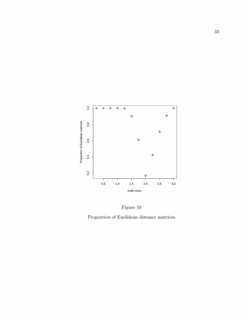
Figure 10
Proportion of Euclidean distance matrices
34
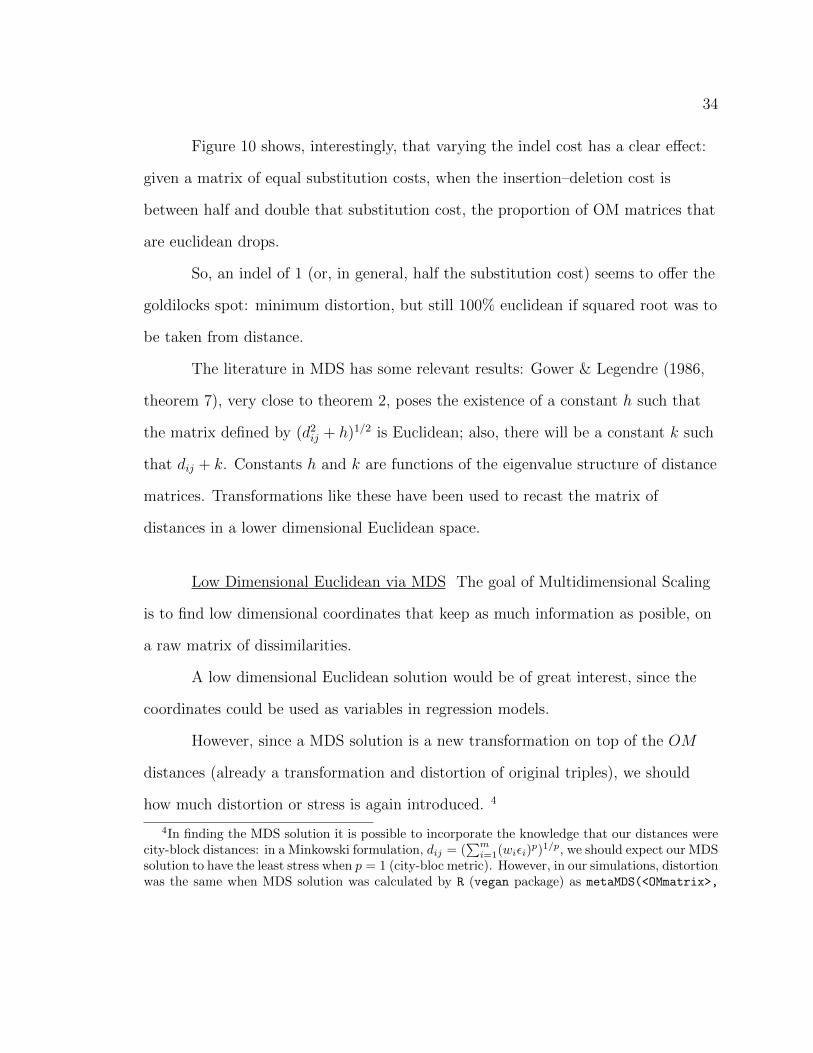
Figure 10 shows, interestingly, that varying the indel cost has a clear effect:
given a matrix of equal substitution costs, when the insertion–deletion cost is
between half and double that substitution cost, the proportion of OM matrices that
are euclidean drops.
So, an indel of 1 (or, in general, half the substitution cost) seems to offer the
goldilocks spot: minimum distortion, but still 100% euclidean if squared root was to
be taken from distance.
The literature in MDS has some relevant results: Gower & Legendre (1986,
theorem 7), very close to theorem 2, poses the existence of a constant h such that
the matrix defined by (d2ij + h)1/2 is Euclidean; also, there will be a constant k such
that dij + k. Constants h and k are functions of the eigenvalue structure of distance
matrices. Transformations like these have been used to recast the matrix of
distances in a lower dimensional Euclidean space.
Low Dimensional Euclidean via MDS The goal of Multidimensional Scaling
is to find low dimensional coordinates that keep as much information as posible, on
a raw matrix of dissimilarities.
A low dimensional Euclidean solution would be of great interest, since the
coordinates could be used as variables in regression models.
However, since a MDS solution is a new transformation on top of the OM
distances (already a transformation and distortion of original triples), we should
how much distortion or stress is again introduced. 4
4In finding the MDS solution it is possible to incorporate the knowledge that our distances werecity-block distances: in a Minkowski formulation, dij = (
∑mi=1(wiεi)
p)1/p, we should expect our MDSsolution to have the least stress when p = 1 (city-bloc metric). However, in our simulations, distortionwas the same when MDS solution was calculated by R (vegan package) as metaMDS(<OMmatrix>,
35
●
●
●
●
●●
●
●●
●
●
●
●●
●
●
●
●●
●
●
●
●
●
●
●
●●
●●
●
●
●●●●●
●
●
●●●
●
●●●
●
●
●●●●
●
●
●
●
●
●
●●●
●
●
●
●●
●●●
●
●
●
●
●●●●
●
●
●●
●
●
●
●●●●
●
●●●
●
●●●●●●
●
●
●●●●●
●
●
●
●
●●●●●●
●●●●●
●
●
●●
●
●
●
●●
●
●
●●
●●●●●
●
●
●●●
●●●
●●
●
●
●
●●
●
●●●●●
●
●●●●
●
●
●
●
●
●
●●
●
●●●●
●
●●●●●●●●●●●●●●●●
●●
●●
●
●●●●●
●
●
●●
●
●●●●●●
●
●
●
●●●● ●●
●
●
●●●
●●●●●●●●●●●●●●●●●●●
●
●
●
●●●●●●
●
●
●●●●●●●●●●●●●●●
●
●●●
●
●
●
●●●●●●
●
●●●●●●●●●●●●●●●●●●●●●●●
●
●●
●
●●
●
●
●
●●●●●
●
●●●●●
●
●●●●● ●●
●
●●●
●●●●●●●
●
●●●●●●●●●●●●●●●●●●●●●●●●●●
●
●
●●
●
●
●●●●●●
●
●●●●●●●●●
●●●●●●●●●●●●●●●●●●●●●●●
●
●●●●●●
●●●●●
●
●●●●●●●
●
●●●●●●●●●●
●
●●●●●●●●●●●●●●●●
●
●●
●
●●●●●●
●
●
●●●●●
●
●
●
●●●
●
●●●
●
●
●●●
●●●●●●
●●
●
●●●●●●●●●●●●●●●●●●●●●●
●
●●
●●●●●●●●●●●
●●●●●●●●●●●●●●●●●
●
●●●●●●●●
●
●●●●●●
●●●●
●
●
●
●
●
●●●●
●
●●●●●●●●●●●●●
●
●
●
●●●●●●●●●
●●●
●●
●
●●●
●●●
●
●
●
●
●●●
●
●●
●
●●●
●
●
●●●
●●●●●●●●●●
●●
●
●●
●
●●●●●●
●
●●●●●●●
●
●
●●●
●
●●●●●●●●●●●●●●
●
●●●●●●●●●●●
●
●●●
●
●
●●
●
●●●
●
●●●●●●●●●●
●
●●
●●●
●
●
●
●
●●●
●
●
●
●●●●●●●●●●
●
●●
●
●●●●●●●●●●●●●●●●●●●
●●
●
●
●
●●●●●
●
● ●●
●●
●
●●●●●
●●●●●●●
●
●
●
●●●●
●●●
●
●●●●●●●●●●●●●●●●●
●
●
●●●●●●
●●●●●●●●
0.25 0.75 1 1.25 1.75 2 2.25 2.75 3
02
46
Cost of Insertion−Deletion
Dis
tort
ion
diffe
renc
e
Figure 11
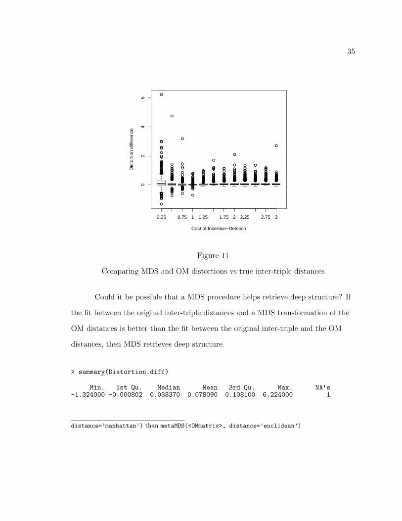
Comparing MDS and OM distortions vs true inter-triple distances
Could it be possible that a MDS procedure helps retrieve deep structure? If
the fit between the original inter-triple distances and a MDS transformation of the
OM distances is better than the fit between the original inter-triple and the OM
distances, then MDS retrieves deep structure.
> summary(Distortion.diff)
Min. 1st Qu. Median Mean 3rd Qu. Max. NA's-1.324000 -0.000802 0.038370 0.078090 0.108100 6.224000 1
distance=’manhattan’) than metaMDS(<OMmatrix>, distance=’euclidean’)

36
Figure 11 and summary shows that the difference in Distortion is a bit
positive – most of the time, the OM representation is closer to the true inter-triple
space than the MDS solution is. The few cases where the MDS solution was an
improvement happened when the indel cost was very low and the OM solution was
already ill fitting (as seen in Figure 9).
The issue of Euclideanity is important because, according to their authors,
some tests depend on that assumption, and the robustness of similar tests is an
active area of discussion (McArdle & Anderson, 2001; Anderson, 2001), as
discussion on how to transform the data (Legendre & Anderson, 1999). Mantel’s
test does not depend on Euclideanity, Permanova neither; MRPP does according to
Mielke & Berry (2001), as did Good (1982).
DISTRIBUTION OF INTER-SEQUENCE DISTANCES
What is the distribution of sequences in a space defined by the Optimal
Matching dissimilarity among them? This question can be split in two questions:
one is about the unidimensional distribution of the inter-sequence OM distance
d(si, sj) = dij. The second is about the distribution in a multidimensional space of
randomly generated sequences, as specified by a matrix of OM distances. For now
we can only explore the first question.
Distribution of True Inter-Triple and OM Distances
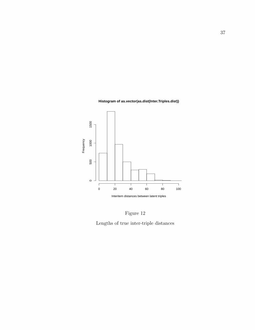
Figure 12 shows the distribution of true inter-triple distances among 100
sequences ((100× 99)/2 = 4950 points in total); graph is censored – there are a few
distances with very large values. Figure 13 shows the distribution of OM distances.
37
Histogram of as.vector(as.dist(Inter.Triples.dist))
Interitem distances between latent triples
Fre
quen
cy
0 20 40 60 80 100
050
010
0015
00
Figure 12
Lengths of true inter-triple distances

38
OM distances
Interitem distances
Fre
quen
cy
0 20 40 60 80
020
040
060
0
Figure 13
Lengths of OM distances
39
MDS solution
Interitem distances
Fre
quen
cy
0 20 40 60 80
010
020
030
040
050
060
0
Figure 14
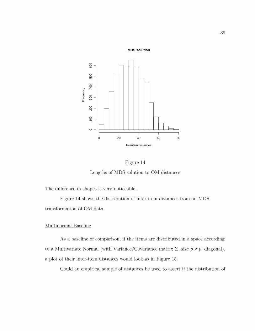
Lengths of MDS solution to OM distances
The difference in shapes is very noticeable.
Figure 14 shows the distribution of inter-item distances from an MDS
transformation of OM data.
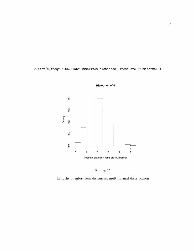
Multinormal Baseline
As a baseline of comparison, if the items are distributed in a space according
to a Multivariate Normal (with Variance/Covariance matrix Σ, size p× p, diagonal),
a plot of their inter-item distances would look as in Figure 15.
Could an empirical sample of distances be used to assert if the distribution of
40
> hist(d,freq=FALSE,xlab="Interitem distances, items are Multinormal")
Histogram of d
Interitem distances, items are Multinormal
Den
sity
0 1 2 3 4 5
0.0
0.1
0.2
0.3
0.4
Figure 15
Lengths of inter-item distances, multinormal distribution

41
inter-sequence OM distances or the MDS solution are roughly equivalent to the one
produced by a multinormal process? It is encouraging that the distribution of
distances produced by the MDS solution is quite close to the multinormal solution.
However we realize that the most important component is not what transformation
of the OM matrix would be the least distorted, of if it is the closest to a well known
distribution, but what transformation would increase the power of tests.

Chapter III
STATISTICAL TESTS FOR INFERENCE
Suppose that the sample of sequences was not from a homogeneous
peopulation, but from a heterogeneous population. For example, some of the
educational/job trajectories correspond to women, some to men. If gender does
affect their trajectory, could the statistic pick that difference as significant (from the
raamdom noise that may be present)? A number of tests will be compared for
power; I will run simulations following Studer et al. (2011), evaluating
� type I error (probability that, in many repetitions of the test, a statistic will
result in values that appear to be inconsistent with the Null Hypothesis of no
group diference, given that there is no such real difference; specifically it will
be a proportion of p-values that are less than a 0.05 threshold, given that the
null hypothesis is true (no difference among subjects by partition).
� statistical power (proportion of times that, in many repetitions of the test, a
statistic will result in values that appear inconsistent with the null hypothesis
of no group difference, given that there is a real difference between groups ;
implemented as the proportion of p-values that are less than a 0.05 threshold,
given that the alternative hypothesis is true).
42

43
MANOVA on Principal Coordinates
In a previous section we saw how an MDS transformation could be used to
obtain a Euclidean version of the OM distance matrix, minimizing distortion and
approaching the distribution of interitem distances by a multinormal distribution.
Given a matrix of distances (size n× n), MDS procedures (principal coordinates
being another name for metric MDS) can be used to obtain a number of coordinates
for every sequence. Such coordinates will be represented in a n× k matrix, where k
is the number of dimensions that was considered to be enough to embody the
variability in the sample; such coordinates can be used as outcome variables, and
explained by categorical explanatory variables, in a MANOVA setting.
Mantel Test
The Mantel test (Mantel, 1967) was initially developed to test for association
between spatial clustering and temporal clustering in cancer cases; in its most basic
form, it uses two square matrices of dissimilarities (or similarities) defined on the
same items – the two matrices are, of course, the same size (n by n), n being the
number of subjects.
In our case, the matrix (Y) can be the matrix of pairwise distances between
sequences; the second matrix (X) can be a matrix of differences between subjects –
the subjects from which the sequences are derived. For instance, it can be a matrix
of absolute age differences, or a matrix of distances generated by some other
trajectory of interest in a state space.
The null hypothesis is that the cells in X are not linearly correlated with the

44
corresponding cells in Y.
Suppose that they were, say, positively correlated. Then the value of
Mantel’s statistic
zM =n−1∑i=1
n∑j=i+1
xijyij
(the sum of the Hadamard product on the lower half of the matrices, not including
diagonals) will be high.
For testing differences between two groups, X can be defined in two
equivalent ways:
� as xij = 0 if sequences i and j belong to the same group, xij = 1 if they belong
to different groups. This coding corresponds to xij as an intuitive measure of
distance – if two objects are in the same group, their distance is 0. As a
consequence,
zM =n−1∑i=1
n∑j=i+1
xijyij =n−1∑i=1
n∑j=i+1
yijεi,j
where indicator function εi,j = 0 if i, j belong to same group, εi,j = 1 if they
belong to different groups. zM then can be defined as the sum of mutual
distances between sequences that do not belong to the same group – a
between-group distance. The alternative hypothesis of clustering by group
would imply that the between-group measure is large. (vec1 is a vector of
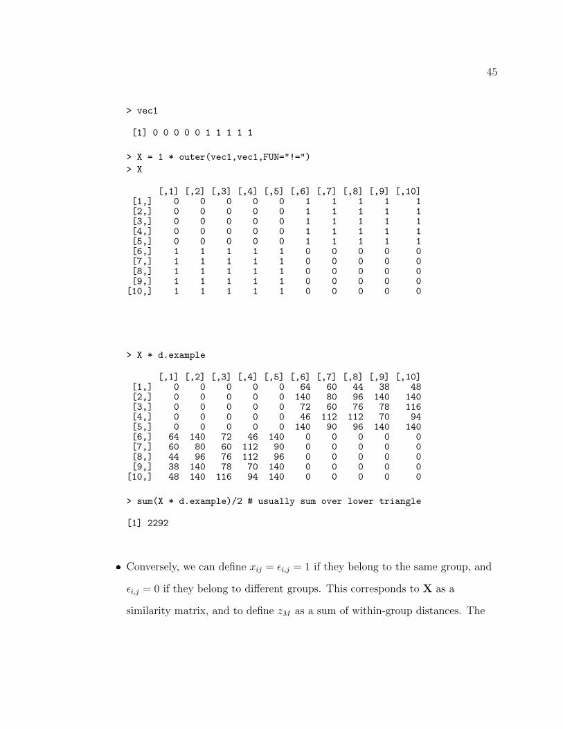
covariate values for every sequence).
45
> vec1
[1] 0 0 0 0 0 1 1 1 1 1
> X = 1 * outer(vec1,vec1,FUN="!=")
> X
[,1] [,2] [,3] [,4] [,5] [,6] [,7] [,8] [,9] [,10][1,] 0 0 0 0 0 1 1 1 1 1[2,] 0 0 0 0 0 1 1 1 1 1[3,] 0 0 0 0 0 1 1 1 1 1[4,] 0 0 0 0 0 1 1 1 1 1[5,] 0 0 0 0 0 1 1 1 1 1[6,] 1 1 1 1 1 0 0 0 0 0[7,] 1 1 1 1 1 0 0 0 0 0[8,] 1 1 1 1 1 0 0 0 0 0[9,] 1 1 1 1 1 0 0 0 0 0[10,] 1 1 1 1 1 0 0 0 0 0
> X * d.example
[,1] [,2] [,3] [,4] [,5] [,6] [,7] [,8] [,9] [,10][1,] 0 0 0 0 0 64 60 44 38 48[2,] 0 0 0 0 0 140 80 96 140 140[3,] 0 0 0 0 0 72 60 76 78 116[4,] 0 0 0 0 0 46 112 112 70 94[5,] 0 0 0 0 0 140 90 96 140 140[6,] 64 140 72 46 140 0 0 0 0 0[7,] 60 80 60 112 90 0 0 0 0 0[8,] 44 96 76 112 96 0 0 0 0 0[9,] 38 140 78 70 140 0 0 0 0 0[10,] 48 140 116 94 140 0 0 0 0 0
> sum(X * d.example)/2 # usually sum over lower triangle
[1] 2292
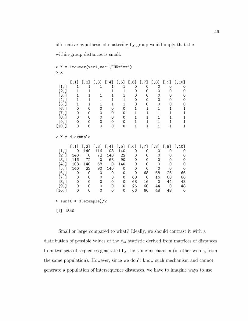
� Conversely, we can define xij = εi,j = 1 if they belong to the same group, and
εi,j = 0 if they belong to different groups. This corresponds to X as a
similarity matrix, and to define zM as a sum of within-group distances. The
46
alternative hypothesis of clustering by group would imply that the
within-group distances is small.
> X = 1*outer(vec1,vec1,FUN="==")
> X
[,1] [,2] [,3] [,4] [,5] [,6] [,7] [,8] [,9] [,10][1,] 1 1 1 1 1 0 0 0 0 0[2,] 1 1 1 1 1 0 0 0 0 0[3,] 1 1 1 1 1 0 0 0 0 0[4,] 1 1 1 1 1 0 0 0 0 0[5,] 1 1 1 1 1 0 0 0 0 0[6,] 0 0 0 0 0 1 1 1 1 1[7,] 0 0 0 0 0 1 1 1 1 1[8,] 0 0 0 0 0 1 1 1 1 1[9,] 0 0 0 0 0 1 1 1 1 1[10,] 0 0 0 0 0 1 1 1 1 1
> X * d.example
[,1] [,2] [,3] [,4] [,5] [,6] [,7] [,8] [,9] [,10][1,] 0 140 116 108 140 0 0 0 0 0[2,] 140 0 72 140 22 0 0 0 0 0[3,] 116 72 0 68 90 0 0 0 0 0[4,] 108 140 68 0 140 0 0 0 0 0[5,] 140 22 90 140 0 0 0 0 0 0[6,] 0 0 0 0 0 0 68 68 26 66[7,] 0 0 0 0 0 68 0 16 60 60[8,] 0 0 0 0 0 68 16 0 44 48[9,] 0 0 0 0 0 26 60 44 0 48[10,] 0 0 0 0 0 66 60 48 48 0
> sum(X * d.example)/2
[1] 1540
Small or large compared to what? Ideally, we should contrast it with a
distribution of possible values of the zM statistic derived from matrices of distances
from two sets of sequences generated by the same mechanism (in other words, from
the same population). However, since we don’t know such mechanism and cannot
generate a population of intersequence distances, we have to imagine ways to use

47
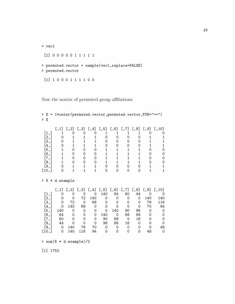
the empirical distance data to imagine a population.
From Legendre & Legendre (1998, p. 554): “According to H0, the vector of
values [distances] observed by any object [sequence] could have been observed by
any other object; in other words, the objects are the permutable units. [...] An
equivalent result is obtained by permuting at random the rows of matrix [X] and
the corresponding columns.”
48
> vec1
[1] 0 0 0 0 0 1 1 1 1 1
> permuted.vector = sample(vec1,replace=FALSE)
> permuted.vector
[1] 1 0 0 0 1 1 1 1 0 0
Now the matrix of permuted group affiliations
> X = 1*outer(permuted.vector,permuted.vector,FUN="==")
> X
[,1] [,2] [,3] [,4] [,5] [,6] [,7] [,8] [,9] [,10][1,] 1 0 0 0 1 1 1 1 0 0[2,] 0 1 1 1 0 0 0 0 1 1[3,] 0 1 1 1 0 0 0 0 1 1[4,] 0 1 1 1 0 0 0 0 1 1[5,] 1 0 0 0 1 1 1 1 0 0[6,] 1 0 0 0 1 1 1 1 0 0[7,] 1 0 0 0 1 1 1 1 0 0[8,] 1 0 0 0 1 1 1 1 0 0[9,] 0 1 1 1 0 0 0 0 1 1[10,] 0 1 1 1 0 0 0 0 1 1
> X * d.example
[,1] [,2] [,3] [,4] [,5] [,6] [,7] [,8] [,9] [,10][1,] 0 0 0 0 140 64 60 44 0 0[2,] 0 0 72 140 0 0 0 0 140 140[3,] 0 72 0 68 0 0 0 0 78 116[4,] 0 140 68 0 0 0 0 0 70 94[5,] 140 0 0 0 0 140 90 96 0 0[6,] 64 0 0 0 140 0 68 68 0 0[7,] 60 0 0 0 90 68 0 16 0 0[8,] 44 0 0 0 96 68 16 0 0 0[9,] 0 140 78 70 0 0 0 0 0 48[10,] 0 140 116 94 0 0 0 0 48 0
> sum(X * d.example)/2
[1] 1752

49
This process could be repeated for all possible permuted assignments of individuals
to groups (n! = 3, 628, 800), or at least for a large enough sample.
Permutational MANOVA
The following graph from Anderson (2001) describes the logic of Anova
testing – if we assume that responses can be in a multidimensional space (and not
just in an unidimensional space).
In our case or sequence comparison, however, our raw data consists of
interpoint distances. Furthermore, a centroid of sequences (“average”) cannot be
easily imagined or defined (same as the average of a set of integer numbers may not
be an integer itself).
50
To solve these difficulties, and if one assumes that distances are metric, there
is a family of approaches that start from the geometrical consideration that variance
and distance are linked by
n∑i=1
(xi − x)2 =1
n
n∑i<j
(xi − xj)2
The right hand is “a sum of the(n2
)pairwise distances among [n points xi]” (Gower
& Krzanowski, 1999).
So it may be possible to reformulate the Anova relationship based on
interpoint distances. I quote from Pillar & Orloci (1996):
“test criterion is the sum of squared dissimilarity between groups:
Qb = Qt −Qw”.
Qt =1
n
n−1∑h=1
n∑i=h+1
d2hi
“which is the total sum of squares involving n(n− 1)/2 pairwise squared
distances (d2hi) between n [objects]. The Qw term is given by
Qw =k∑
c=1
Qwc
This is the sum of squares within the k groups. The terms in Qw accord
with
Qwc =1
nc
n−1∑h=1
n∑i=h+1
d2hiδ(h, i, c)
which is the sum of squares within group c with size nc. The indicator
variable δ(h, i, c) is one if [objects] h and i belong to group c or zero if
51
otherwise.
How do we evaluate the significance of an F ratio in a multidimensional
distance setting? Under the null hypothesis the allocation of objects to groups
would not matter, so objects could be randomly allocated or permuted to groups,
and a distribution of pseudo-F values computed.
The problem of evaluating the significance of a pseudoF to distinguish
among groups is different from the problem of partitioning variability – defined as
“attributing additive proportions of the total variability to individual factors in an
experimental design” (McArdle & Anderson, 2001) when the measure of distance is
not metric. Statistics for the first problem are already well known (Mantel, 1967;
Good, 1982; Dietz, 1983; Clarke, 1993) and as we will show, mostly equivalent.
On the other hand, the issue of partitioning, particularly in multifactorial
models, is not completely understood. When decomposing a semimetric distance
matrix, by means of principal coordinate analysis, into a linear set of Euclidean
coordinates, the result may contain imaginary Euclidean coordinates or negative
eigenvalues, of unclear interpretation. McArdle & Anderson (2001); Anderson
(2001); Reiss et al. (2010) propose to avoid any correction (advocated by Legendre
& Anderson (1999)) and work directly with the data.
Permanova’s statistic, in the simplest balanced design (same number n of
52
items per group) is
F =SSA/(a− 1)
SSW/(N − a)where SSA = SST − SSW ,
SST =1
N
N−1∑i=1
N∑j=i+1
d2ij
SSW =1
n
N−1∑i=1
N∑j=i+1
d2ijεij
where εij = 1 if item i and j belong to the same group, 0 otherwise.
The permutational strategy to test for significance of the statistic is the same
as for Mantel’s.
MRPP
In the original notation of Mielke & Berry, MRPP statistic is
δ =
g∑i=1
Ciξi
where
ξi =
(ni
2
)−1∑I<J
∆I,JΨi(ωI)Ψi(ωJ)
i is every one of the groups, from 1 to g. ni is the number of items in group i,(ni
2
)divides by the number of symmetric pairs in a group of size ni.
∑I,J represents a
sum of terms over a lower triangle. Ψi(ωI) = 1 if object ωI belongs to group Si. So
Ψi(ωI)Ψi(ωJ) is an indicator function with a value of 1 if objects ωI and ωJ belong
to same group Si. Ci is a weight coefficient that can be defined many ways; Mielke
(1985) recommends the proportion of items in group i, Ci = ni/N , and criticizes
53
other choices implicit in the literature, as inefficient.
∆I,J is an dissimilarity defined as
dI,J = [r∑
h=1
(xhI − xhJ)2]v/2
where the value v is left to the theoretical choice of the researcher. If xhI , xhJ are
coordinates, and v = 1, ∆I,J is an Euclidean distance. Note how with v = 2, ∆I,J
may violate the triangle inequality (as an example in one-dimensional space, if
x1 = 4, x2 = 6, x3 = 7, then ∆12 = 4,∆13 = 9,∆23 = 1 and ∆12 + ∆23 < ∆13,
violating triangle inequality). Mielke & Berry call for congruence between the data
space (Euclidean in this case) and the statistical method’s analysis space. Authors
note to the existence of counterintuitive results caused by the use of v = 2. Mielke
& Berry (2001) explored power of tests to detect location shifts, as affected by
different values of v, across many unidimensional distributions. In cases where the
underlying distribution is not known, authors defend the choice of v = 1.
A rewrite of MRPP’s statistic, closer to the formulas for Mantel’s and
Permanova, would be
δ =
g∑k=1
nk
N
2
nk(nk − 1)
N−1∑i=1
N∑j=i+1
dijεij
(Mielke & Berry would make group weight Ck = nk/K, where K is the total number
of items classified in groups – there may be items not classified, N −K ≥ 0; however,
for simplification, we assume that all items are classified and that K = N . )
For MRPP, permutational testing is done in an similar way than Mantel’s –

54
with a caveat: possible allocations of N objects to the g + 1 groups (the [g + 1]th
group being the excess group or residual category), would be
M =N !∏g+1
k=1 nk!
(This is more precise than the N ! from Mantel’ s description).

Chapter IV
A COMPARISON OF POWER
GENERAL STRATEGY
Simulations will be used to investigate the power of some statistical tests. In
each simulation run, two sets of sequences will be generated: the baseline set and
the alternate set.
To investigate Type I error, in every simulation run, these two sets are
generated from the same mechanism with the same parameter values. In other
words, they come from the same population – null hypothesis H0 is true. Out of
many simulations, how often will the test be mistaken? (by the statistic value being
in the rejection region, leading to the mistaken interpretation that they would come
from different populations.)
To investigate power, in every simulation run, the alternate set and the
baseline set are generated from different parameters – each set comes from different
populations. Out of many simulations, how often will the test be able to detect that
they, in fact, come from two different populations – how often will the value of the
statistic be in the rejection region?
For each simulation run, a total of 30 sequences will be generated; 15
sequences in the baseline set, and 15 in the alternate set.
At every one of the 2000 simulation runs, the tests (non-parametric like
55

56
Mantel and Permutational MANOVA, parametric like tests of means and medians)
will be applied on the same pair of sets (baseline and alternate).
The process will be repeated, across a range of progressively more distant
values of alternate parameters (from baseline parameters).
Making Use of Parametric Information
The focus of this research is on a number of non-parametric tests that do not
assume previous knowledge about how sequences are generated. However, it may be
interesting to compare the performance of such non-parametric tests with the
performance of tests that made use of our knowledge about the stochastic generator
of the sequences.
Suppose that we knew much more about the generating mechanism. In this
case, going back to Chapter II, notice that the parameters that generate the first
and third preliminary sequences are fixed, and we only change the value of
parameters for the mechanism acting on the second sequence.
If we only observed resulting data, but knew that the key piece of information
was the change in t2, we could identify the footprint of that change, by realizing that
when a state switched from (Z,0,Z) to (Z,1,Z), the inflection point has happened.
We know that the switch has happened in the final sequence, when one of
these listed sub-sequences shows up. In parenthesis we see the triple representation
of the digits. Notice how the central 0 switches to 1.
� sub-sequence ...02... (state 000 became 010),
� ...03... (000→ 011),
57
� ...06... (000→ 110),
� ...07... (000→ 111),
� ...13... (001→ 011),
� ...17... (001→ 111),
� ...46... (100→ 110),
� ...47... (100→ 111),
� ...57... (101→ 111).
For each sequence we can get a number that indicates where any such pair
shows up in the sequence. Suppose the sequence was 00000022, the value of interest
will be 7, since 7th is the place where the transition shows up (the place of the “2”
after “0”). For each sequence, let us call this value its observed transition value.
A set of n sequences, be the baseline or the alternate, would provide a vector
(size n) of observed transition values. If the sub-sequence never happens in a
sequence, because the randomly generated value for t2 was larger than the sequence
length, we can consider that the transition value is missing.
The vector of the transition values from baseline set can be compared with
the vector of the transition values from the alternate set; two straightforward tests
that come to mind are a 2-sample t tests, and a permutational test of difference of
medians.
It seems reasonable to expect that these two tests will be more powerful than
the Mantel, Permanova or MRPP tests, since they incorporate more knowledge
about how the sequences were generated and what footprint to look for.

58
SIMULATION
Optimal matching needs a matrix of penalty costs for the transition between
state i to j. (Note that for our particular generator, some values in the transition
matrix will be of no use, since some transitions cannot occur, like 011 to 010: once a
member of a triple becomes 1, it stays that way, it cannot go back to a 0 value.
However, since we ignore that fact, all substitution costs are assumed to be
constant.)
> cost.matrix
[,1] [,2] [,3] [,4] [,5] [,6] [,7] [,8][1,] 0 2 2 2 2 2 2 2[2,] 2 0 2 2 2 2 2 2[3,] 2 2 0 2 2 2 2 2[4,] 2 2 2 0 2 2 2 2[5,] 2 2 2 2 0 2 2 2[6,] 2 2 2 2 2 0 2 2[7,] 2 2 2 2 2 2 0 2[8,] 2 2 2 2 2 2 2 0
R packages were used: ape (Paradis, Claude, & Strimmer, 2004), ecodist
(Goslee & Urban, 2007), vegan (Oksanen et al., 2013).
59
Changing Start Parameter, Fixing Rate
In this mechanism defined by a multiple log-logistic model, we’ll be
comparing reference sequences generated by
t1 = 0 + LL(Rate = 0.078, Shape = 2.364)
t2 = 10 + LL(Rate = 0.126, Shape = 2.364)
t3 = 20 + LL(Rate = 0.078, Shape = 2.364)
with sequences generated by
t1 = 0 + LL(Rate = 0.078, Shape = 2.364)
t2 = a2 + LL(Rate = 0.126, Shape = 2.364)
t3 = 20 + LL(Rate = 0.078, Shape = 2.364)
where the Start parameter a2 increases from 10 (Null Hypothesis is true) to 15.
Figure 16 shows the power function of various statistics. Power function is
defined as the probability of the statistic being in the rejection region, given data
generated from a mechanism with such parameter value (Start in this case).
Baseline set is generated with Start=10, alternative sets are generated from
increasing values of Start. At first, the two sets are both generated from Start=10 –
they come from the same population. Probability of rejecting the null hypothesis,
given that Start=10, is the Type I error. We see how the lines are concentrated a
bit over 0, perhaps around 0.05 – this is in agreement with a tolerable type I error.

60
M M M M M M M MM
M
10 11 12 13 14 15
0.0
0.2
0.4
0.6
0.8
1.0
Start parameter
% o
f p−
valu
es <
.05
P P P P P PP P
PP
* * * * * ** *
**
t t tt
tt
t
t
t
t
+ + ++
++
+
+
+
+
m m m m m m m mm m
MP*t+m
MantelPermanovaMRPPt truncateddiff mediansMANOVA on PCoA
Figure 16
Power of tests, by values of Start parameter (Rate fixed)
As the alternate sets are generated by more divergent Start values, the power
to detect that they are not from the same baseline population increases – as
expeted. However we see how the non-parametric tests are less powerful than the
ones that make use of parametric information.
Figure 16 shows that the parametric tests (t truncated, and difference of
means, based on inside knowledge about the parameter of interest and footprint to
follow to identify differing sequences) have the most power. The non-parametric
permutational tests have less power. The MANOVA test done on a euclidean
transformation of the OM solution has the least power of the compared tests.
61
Changing Rate (Keeping Start Fixed)
Now we are comparing reference sequences generated by
t1 = 0 + LL(Rate = 0.078, Shape = 2.364)
t2 = 10 + LL(Rate = 0.078, Shape = 2.364)
t3 = 20 + LL(Rate = 0.078, Shape = 2.364)
with sequences generated by
t1 = 0 + LL(Rate = 0.078, Shape = 2.364)
t2 = 10 + LL(Rate = λ2, Shape = 2.364)
t3 = 20 + LL(Rate = 0.078, Shape = 2.364)
where 0.078 ≤ λ2 ≤ 0.205.
The inverse of the Rate (aka Intensity) parameter in a log-logistic
distribution is called the Scale parameter; such Scale parameter happens to be the
median of the distribution. So a natural estimator for Rate is the inverse of the
median of a sample.
However, if we are not really dealing with a continuous log-logistic
distribution, but with a discretized log-logistic (since we do not observe the actual
random quantity T , but the integer X that is equal or greater than T ) the
distribution of medians of discretized random quantities may not have enough
granularity.
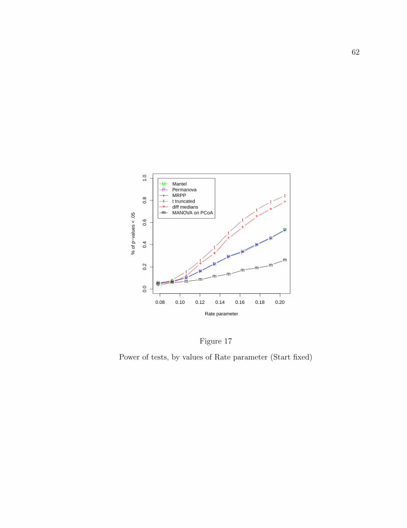
62
M MM
MM
MM
MM
M
0.08 0.10 0.12 0.14 0.16 0.18 0.20
0.0
0.2
0.4
0.6
0.8
1.0
Rate parameter
% o
f p−
valu
es <
.05
P PP
P
P
PP
P
P
P
* **
*
*
**
**
*
tt
t
t
t
t
t
t
tt
++
+
+
+
+
+
+
+
+
m m m mm m
m m mm
MP*t+m
MantelPermanovaMRPPt truncateddiff mediansMANOVA on PCoA
Figure 17
Power of tests, by values of Rate parameter (Start fixed)

63
Same with previous comparison, Figure 17 shows that the parametric tests (t
truncated, and difference of means, based on inside knowledge) have the most
power. The non-parametric permutational tests have less power. The MANOVA
test done on a euclidean transformation of the OM solution has the least power of
the compared tests.
The Effect of Length of Sequence in Power of Tests
We saw in subsection (page 63) that distorion decreases as sequence length
increases, as expected.
Could we expect that power increases with sequence length? In the
simulated sequences, half come from a baseline population where Start=10, half
come from a popuation where Start=15; Rate parameter is fixed.
Figure 18 shows that, surprisingly, power seems to go down, the longer the
sequences are. To better understand this result, we should review some findings and
conclusions:
� Should length of strings (sequences) affect raw edit distance? All other things
being equal, yes, since a tranformation from one string to another would need
more insertions or substitutions.
� Should length of string affect a Mantel-type statistic? no: while it would affect
the computed value of the specific statistic, it should not affect the evaluation
of significance – the distribution of permuted statistics should still be
equivalent. If distance matrix is [dij], a statistic calculated on a transformed
[d∗ij] should not change in power.

64
M
MM M
25 30 35 40 45 50 55 60
0.0
0.2
0.4
0.6
0.8
1.0
Sequence Length
% o
f p−
valu
es <
.05
P
PP P
*
** *
t
t
tt+ + + +
mm
m m
MP*t+m
MantelPermanovaMRPPt truncateddiff mediansMANOVA on PCoA
Figure 18
Power of tests, by length of sequences (Start and Rate fixed)

65
� should length of sequences affect the distortion between [dij] (the matrix of
Levenshtein-like distances among sequences) and [δij (the matrix of true
euclidean distances between original triples)? As seen before, Distortion
decrease with increased sequence length. With shorter sequence lengths (for
example, with length 40) some triples that are truly different (say triples
10,15,42 and 10,15,50) would still produce the same final sequence. If length
was 50, the triples would produce different sequences. Differentiation of
previous outliers is a way in which increased length lessens distortion.
However, if we take outlier differentiation out of the table, would length still
increase power? To verify that, we can write the simulation by generating
sequences, but discarding those triples where one or more of the three components is
greater than the sequence length. So there would be no outliers in the triples.
Figure 19 shows that power does go down even more with length.

66
M
MM M
25 30 35 40 45 50 55 60
0.0
0.2
0.4
0.6
0.8
1.0
Sequence Length
% o
f p−
valu
es <
.05
P
PP P
*
** *
t
tt
t
++
+ +
m
m m m
MP*t+m
MantelPermanovaMRPPt truncateddiff mediansMANOVA on PCoA
Figure 19
Power by Seq Length, keeping triples truncated
Chapter V
ANALYTICAL IDENTITY BETWEEN MANTEL AND PERMANOVA
Why should Mantel, Permanova and MRPP produce identical results?
Remember how Mantel’s statistic in our case of two group comparison was
N−1∑i=1
N∑j=i+1
dijεi,j
where εi,j is an indicator variable with value 1 if item i and j belong to the same
original group, 0 otherwise.
MRPP’s statistic was
δ =
g∑k=1
Ck2
nk(nk − 1)
N−1∑i=1
N∑j=i+1
∆ijεi,j
where εi,j is defined as before (1 if both i, j ∈ k group), and ∆i,j = dvi,j and usually
v = 1.
As nk is a constant in this case, Mantel and MRPP, at least in this very
simple case, when v = 1, are analytically equivalent. Furthermore, raising dvij to a
v = 2, for instance, would make it a monotonous transformation of dij, with
unchanged distributional properties.
For Permanova, statistic of interest was (Anderson, 2001):
67

68
F =SSA/(a− 1)
SSW/(N − a)=SSA
SSW
N − aa− 1
The term N−aa−1 (where a represents number of groups and N total number of items)
is invariant.
SSA
SSW
=SST − SSW
SSW
=SST
SSW
− 1
SST is invariant over all possible permutations, so statistic is only a function of
SSW .
As
SSW =1
n
N−1∑i=1
N∑j=i+1
d2ijεij
We have shown that Permanova’ s statistic, under these simple conditions, and
given the same data, has the same distributional properties as Mantel’s and MRPP.
Chapter VI
CONCLUSIONS
Optimal Matching distances have been used to explore categorical sequences;
in rcent times a more careful consideration of statistical inference has been
attempted Studer et al. (2011).
Given a known distribution of random objects (triples), and given an
algorithm that generates sequences from such triples, this study looked at how
distorted was the OM representtaion vis a vis the original. We find that OM costs
affect the distortion, and that an indel cost valued at half of substitution costs
produce the least amount of distortion. We also found that the longer the sequences,
the less distorted the OM distances were from the original. We found that the
distances were metric, but not Euclidean. Given the OM distances, an Euclidean
aproximation could be found by computing the square root of the values, or even
better, by finding an MDS solution. MDS solutions also had the nice property of
producing a distribution of distances that was quite close to the euclidean distances
from items that came from a Multivariate Normal distribution of items.
Not surprisingly, permutational tests like MRPP, Mantel and Permanova
were less powerful than tests based on insight about the parametric generation of
the sequences. Surprisingly, a MANOVA test on the MDS solution had very weak
power. Surprisingly also, power was decreased by an increase in the sequence length.
69

70
At his point we do not have a good explanatory mechanism for this result.
Since Permanova (Anderson, 2001) explicitly addresses the issue of multiway
analysis of discrepancy, practical researchers are encouraged to follow Dr.
Anderson’s work and tools. However, researchers need to be aware that the power of
these tests is low.
FUTURE WORK
It will be necessary to study if results are robust across sequences derived
from other generators. Second, there are two other tests that I discovered very late
in the process: DISCO (Rizzo & Szekely, 2010) and crossmatch (Rosenbaum, 2005),
based on work by Friedman & Rafsky (1983). This last one is of particular interest
because it is based on minimal spanning trees, an area of work very close to Joe
Kruskal. 1 These may or may not be as powerful or extendable as Anderson’s, so
more research is needed to compare their power.
We can expect more theoretical work on the issue of non-euclideanity and
how it affects inference, going beyond Gower & Legendre (1986); Legendre &
Anderson (1999); McArdle & Anderson (2001).
1It is a mistery how Kruskal, who was involved in both MDS and Optimal Matching, neverseemed to have combined the two.

REFERENCES
71
REFERENCES
Abbott, A. (2000, August). Reply to Levine and Wu. Sociological Methods andResearch, 29 (1), 65–76.
Abbott, A., & Forrest, J. (1986, winter). Optimal matching methods for historicalsequences. Journal of Interdisciplinary History , 16 (3), 471–494.
Abbott, A., & Hrycak, A. (1990). Measuring resemblence in sequence data: Anoptimal matching analysis of musicians careers. American Journal of Sociology ,96 (1), 144–185.
Abbott, A., & Tsay, A. (2000, August). Sequence analysis and optimal matchingmethods in sociology. Sociological Methods & Research, 29 (1), 3–33.
Anderson, M. J. (2001). A new method for non-parametric multivariate analysis ofvariance. Austral Ecology , 26 , 32–46.
Blossfeld, H.-P., & Rohwer, G. (2002). Techniques of event history modeling. Newapproaches to causal analysis (2nd ed.). Mahwah, NJ: Lawrence ErlbaumAssociates.
Borg, I., & Groenen, P. J. F. (2005). Modern multidimensional scaling: Theory andapplications (2nd ed.). New York: Springer.
Clarke, K. R. (1993). Non-parametric multivariate analyses of changes incommunity structure. Australian journal of Ecology , 18 , 117-143.
Dietz, E. J. (1983, March). Permutation tests for association between two distancematrices. Systematic Zoology , 32 (1), 21–26.
Diggle, P. J., Liang, K.-Y., & Zeger, S. L. (1994). Analysis of longitudinal data.Oxford (England): Oxford University Press.
Dutang, C., Goulet, V., & Pigeon, M. (2008). actuar: An R package for actuarialscience. Journal of Statistical Software, 25 (7), 38. Retrieved fromhttp://www.jstatsoft.org/v25/i07
Elzinga, C. H. (2010). Complexity of categorical time series. Sociological Methods &Research, 38 (3), 463–481.
72

73
Friedman, J. H., & Rafsky, L. C. (1983). Graph-theoretic measures of multivariateassociation and prediction. The Annals of Statistics , 11 (2), 377–391.
Gabadinho, A., Ritschard, G., Muller, N. S., & Studer, M. (2011, 4 7). Analyzingand visualizing state sequences in R with TraMineR. Journal of StatisticalSoftware, 40 (4), 1–37. Retrieved from http://www.jstatsoft.org/v40/i04
Gauthier, J.-A., Widmer, E. D., Bucher, P., & Notredame, C. (2009). How muchdoes it cost? optimization of costs in sequence analysis of social science data.Sociological Methods and Research, 38 (1), 197–231.
Good, I. J. (1982). An index of separateness of clusters and a permutation test forits significance. Journal of Statistical Computation and Simulation, 15 , 81–84.
Goslee, S. C., & Urban, D. L. (2007). The ecodist package for dissimilarity-basedanalysis of ecological data. Journal of Statistical Software, 22 , 1-19.
Gower, J. C., & Krzanowski, W. J. (1999). Analyses of distance for structuredmultivariate data and extensions to multivariate analysis of variance. AppliedStatistics , 48 , 505–519.
Gower, J. C., & Legendre, P. (1986). Metric and euclidean properties ofdissimilarity coefficients. Journal of classification, 3 , 5–48.
Gusfield, D. (1997). Algorithms on strings, trees, and sequences: computer scienceand computational biology. Cambridge (England): Cambridge University Press.
Hubert, L. J., & Schultz, J. (1976). Quadratic assignment as a general data analysisstrategy. British Journal of Mathematical and Statistical Psychology , 29 ,190–241.
Kaufman, L., & Rousseeuw, P. J. (1990). Finding groups in data : an introductionto cluster analysis. New York: Wiley.
Klein, J. P., & Moeschberger, M. L. (2007). Survival analysis. techniques forcensored and truncated data (2nd ed.). New York: Springer.
Krause, E. F. (1975). Taxicab geometry: an adventure in non-euclidean geometry.New York: Dover Publications.
Kruskal, J. B., & Wish, M. (1978). Multidimensional scaling. Beverly Hills andLondon: Sage Publications.
Legendre, P., & Anderson, M. J. (1999). Distance-based redundance analysis:testing multi-species responses in multi-factorial ecological experiments.Ecological Monographs , 69 , 1–24.

74
Legendre, P., & Legendre, L. (1998). Numerical ecology (Second English ed.).Amsterdam: Elsevier.
Lesnard, L. (2010). Setting cost in optimal matching to uncover contemporaneoussocio-temporal patterns. Sociological Methods and Research, 38 (3), 389–419.
Levine, J. H. (2000). But what have you done for us lately? commentary on Abbottand Tsay. Sociological Methods and Research, 29 (1), 34–40.
Macindoe, H., & Abbott, A. (2003). Handbook of data analysis. In M. Hardy &A. Bryman (Eds.), (chap. Sequence Analysis and Optimal Matching Techniquesfor Social Science Data). London: SAGE.
Manly, B. F. J. (1997). Randomization, bootstrap and monte carlo methods inbiology (Second ed.). London: Chapman & Hall.
Mantel, N. (1967). The detection of disease clustering and a generalized regressionapproach. Cancer Research, 27 (2), 209–220.
McArdle, B. H., & Anderson, M. J. (2001). Fitting multivariate models tocommunity data: a comment on distance-based redundancy analysis. Ecology ,82 (1), 290–297.
McVicar, D., & Anyadike-Danes, M. (2002). Predicting successful and unsuccessfultransitions from school to work by using sequence methods. Journal of the RoyalStatistical Society. Series A (Statistics in Society), 165 (2), 317–334.
Mielke, P. W., Jr. (1985). Multiresponse permutation procedures. In S. Kotz &N. L. Johnson (Eds.), Encyclopedia of statistical sciences vol. 5 (pp. 724–727).John Wiley and Sons.
Mielke, P. W., Jr, & Berry, K. J. (2001). Permutation methods. A distance basedapproach (First ed.). New York: Springer.
Oksanen, J., Blanchet, F. G., Kindt, R., Legendre, P., Minchin, P. R., O’Hara,R. B., . . . Wagner, H. (2013). vegan: Community ecology package [Computersoftware manual]. Retrieved from http://CRAN.R-project.org/package=vegan(R package version 2.0-8)
Paradis, E., Claude, J., & Strimmer, K. (2004). APE: analyses of phylogenetics andevolution in R language. Bioinformatics , 20 , 289-290.
Pillar, V. D. P., & Orloci, L. (1996, Aug). On randomization testing in vegetationscience: Multifactor comparisons of releve groups. Journal of Vegetation Science,7 (4), 585–592.
75
R Core Team. (2012). R: A language and environment for statistical computing[Computer software manual]. Vienna, Austria. Retrieved fromhttp://www.R-project.org/ (ISBN 3-900051-07-0)
Reiss, P. T., Henry, M., Stevens, H., Shehzad, Z., Petkova, E., & Milham, M. P.(2010). On distance-based permutation tests for between-group comparisons.Biometrics , 66 , 636–643.
Rizzo, M. L., & Szekely, G. J. (2010). DISCO analysis: a nonparametric extensionof analysis of variance. The Annals of Applied Statistics , 4 (2), 1034–1055.
Rosenbaum, P. R. (2005). An exact distribution-free test comparing twomultivariate distributions based on adjacency. Journal of the Royal StatisticalSociety: Series B (Statistical Methodology), 67 (4), 515-530.
Sankoff, D., & Kruskal, J. B. (Eds.). (1983). Time warps, string edits andmacromolecules. Reading, MA: Addison-Wesley.
Studer, M., Ritschard, G., Gabadinho, A., & Muller, N. S. (2011, August).Discrepancy analysis of state sequences. Sociological Methods and Research,40 (3), 471–510.
Ware, J. H., & Lipsitz, S. (1988). Issues in the analysis of repeated categoricaloutcomes. Statistics in Medicine, 7 , 95–107.
Wilson, C. (2006). Reliability of sequence-alignment analysis of social processes:Monte Carlo tests of ClustalG software. Environment and Planning A, 38 ,187–204.
Wu, L. L. (2000, August). Some comments on “Sequence Analysis and OptimalMatching Methods in Sociology: Review and Prospect”. Sociological Methods andResearch, 29 (1), 41–64.
Yamaguchi, K. (1991). Event history analysis. Newbury Park, Calif.: Sage.

APPENDICES
76

APPENDIX A
Parallelizing the code
77

78
Using multiple CPU cores may speed up the code. In this case the packages
multicore and doMC will be used.
To parallelize a computation means to divide the computation in parts and
send each part to be run by a separate CPU core. Each time a CPU core finishes a
job, communicates to the main process, and starts a new job, it spends precious
time. If we were to send very many small jobs to a limited number of cores, too
much time would be spent. For this reason, given few CPU cores (8 in our case) it is
better to divide the job by partial jobs, and send each partial job to each core.
In this examination of the power of tests, we are calculating the proportion
of tests that reject a null hypothesis, for a given parameter value. As an example,
when analyzing the effect of varying the start parameter on power, the parameter
can take values of
[1] 10.00000 10.55556 11.11111 11.66667 12.22222 12.77778 13.33333 13.88889[9] 14.44444 15.00000
For each of these values the code will generate 2000 tests, each test done on
sets of 30 each. So, a good way to divide the total computation is by using the 10
values of the start parameter, by creating 10 subjobs and allocating each to every
CPU core.
This R code describes the process:
range.a2 <- seq(from=10,to=15,length.out=NumberOfSteps)
values <- foreach (fa.second = range.a2, .combine=rbind) %dopar%
{SimulateSequences(..., a2=fa.second) }

79
As said, range.a2 defines the vector of possible values for the start
parameter. fa.second is that same vector – foreach needs it like that to be
digested. The pair foreach %dopar% allocates the job (SimulateSequences()) to
each available core, by each value of fa.second (called a2 when passed to
SimulateSequences()). The function SimulateSequences() generates sequences
and runs the tests, using some parameter values, among them, the passed value for
a2.

APPENDIX B
Checking for correctness of Distortion measure
80

81
The distortion or stress measure should be valid.
For example, suppose that some triples are generated with our mechanism.
> numSequences=10
> Simulated=generateManySequences(mySequenceLength=30,
+ myNumSeqs=numSequences,
+ myStart=10,myIntensity=0.126)
> Triples= Simulated[[2]]
> Triples
t1 t2 t3[1,] 7.155893 23.45470 35.20091[2,] 13.054163 21.09227 41.14212[3,] 14.060573 14.71772 36.94382[4,] 9.961945 18.95285 36.70726[5,] 12.852642 11.56148 23.91011[6,] 18.236457 64.29956 52.06315[7,] 10.416711 23.31193 27.66013[8,] 9.194970 13.02532 49.50518[9,] 32.386538 16.00019 26.55220[10,] 22.307891 18.15877 33.03406
From that rectangular matrix of triples, n× 3, an n× n square matrix of
interitem distances is calculated. This will be our original distance matrix.
> Euc.dist = as.matrix(dist(Triples,method="euclidean"))
> round(Euc.dist,2)
1 2 3 4 5 6 7 8 9 101 0.00 8.70 11.27 5.51 17.36 45.56 8.22 17.82 27.69 16.202 8.70 0.00 7.70 5.81 19.69 44.87 13.92 12.24 24.75 12.653 11.27 7.70 0.00 5.90 13.46 52.00 13.17 13.58 21.11 9.754 5.51 5.81 5.90 0.00 15.06 48.59 10.05 14.12 24.79 12.915 17.36 19.69 13.46 15.06 0.00 60.02 12.57 25.90 20.21 14.706 45.56 44.87 52.00 48.59 60.02 0.00 48.34 52.13 56.43 50.087 8.22 13.92 13.17 10.05 12.57 48.34 0.00 24.18 23.18 14.038 17.82 12.24 13.58 14.12 25.90 52.13 24.18 0.00 32.76 21.679 27.69 24.75 21.11 24.79 20.21 56.43 23.18 32.76 0.00 12.1810 16.20 12.65 9.75 12.91 14.70 50.08 14.03 21.67 12.18 0.00
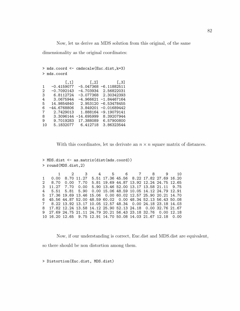
82
Now, let us derive an MDS solution from this original, of the same
dimensionality as the original coordinates:
> mds.coord <- cmdscale(Euc.dist,k=3)
> mds.coord
[,1] [,2] [,3]1 -0.4159077 -5.047368 -6.118825112 -0.7092143 -4.703934 2.568220313 6.8112724 -3.077368 2.303423934 3.0675944 -4.966621 -1.844671645 14.9854840 2.953120 -6.534784556 -44.6768806 3.849201 -0.016894427 2.7429013 1.888164 -9.190791418 3.3096144 -14.695999 8.392079449 9.7019283 17.388089 6.5790080010 5.1832077 6.412718 3.86323544
With this coordinates, let us derivate an n× n square matrix of distances.
> MDS.dist <- as.matrix(dist(mds.coord))
> round(MDS.dist,2)
1 2 3 4 5 6 7 8 9 101 0.00 8.70 11.27 5.51 17.36 45.56 8.22 17.82 27.69 16.202 8.70 0.00 7.70 5.81 19.69 44.87 13.92 12.24 24.75 12.653 11.27 7.70 0.00 5.90 13.46 52.00 13.17 13.58 21.11 9.754 5.51 5.81 5.90 0.00 15.06 48.59 10.05 14.12 24.79 12.915 17.36 19.69 13.46 15.06 0.00 60.02 12.57 25.90 20.21 14.706 45.56 44.87 52.00 48.59 60.02 0.00 48.34 52.13 56.43 50.087 8.22 13.92 13.17 10.05 12.57 48.34 0.00 24.18 23.18 14.038 17.82 12.24 13.58 14.12 25.90 52.13 24.18 0.00 32.76 21.679 27.69 24.75 21.11 24.79 20.21 56.43 23.18 32.76 0.00 12.1810 16.20 12.65 9.75 12.91 14.70 50.08 14.03 21.67 12.18 0.00
Now, if our understanding is correct, Euc.dist and MDS.dist are equivalent,
so there should be non distortion among them.
> Distortion(Euc.dist, MDS.dist)

83
[1] 7.579766e-16
●
●
●
●
●
●
●
●
●
●
●
●
●
●●
●
●
●
●
●
●●
●
●
●
●
●
●
●
●
●
●
●
●
●
●
●
●
●
●●
●
●
●
●
10 20 30 40 50 60
1020
3040
5060
Euclidean Distances
MD
S d
ista
nces
Distortion measure is 0, and Shepard plot show a diagonal line, meaning
there was no distortion, as expected.
As a further check, let us add a random quantity to the distances, to
convince ourselves that the stress calculation holds for progressively more distorted
matrices. To distort them, we add matrices of random values to it.
> distorted.a.bit = matrix(runif(n=100,min=0,max=5),nrow=10,ncol=10)
> distorted.a.lot = matrix(runif(n=100,min=0,max=20),nrow=10,ncol=10)
> distorted.a.wholelot = matrix(runif(n=100,min=0,max=40),nrow=10,ncol=10)
> Distortion(Euc.dist,(MDS.dist+distorted.a.bit))
[1] 0.1120655
> Distortion(Euc.dist,(MDS.dist+distorted.a.lot))
[1] 0.4395485

84
> Distortion(Euc.dist,(MDS.dist+distorted.a.wholelot))
[1] 0.8698769
As expected, the computed value of Distortion increases with increasingly
distorted matrices.

APPENDIX C
R source code
85

86
This section contains the code that was run.
1 ### R code from v i g n e t t e source ' IntroToGenera lStrat .Rnw'
23 ###################################################4 ### code chunk number 1 : IntroToGenera lStrat .Rnw:17−195 ###################################################6 l ibrary (TraMineR)7 #se t . seed (123)89
10 ###################################################11 ### code chunk number 2 : t r y12 ###################################################13 data (mvad)14 mvad . lab = c ( ”Employed ” , ”Further Education ” , ”Higher Education ” , ”
J o b l e s s ” , ”In School ” , ”Train ing ”)15 mvad . scode = c ( ”EM” , ”FE” , ”HE” , ”JL” , ”SC” , ”TR”)16 mvad . seq = seqde f (mvad , 1 7 : 8 6 , s t a t e s=mvad . scode , labels=mvad . lab , x t s t ep
=6)17 s e q i p l o t (mvad . seq , border=NA)181920 ###################################################21 ### code chunk number 3 : t r an s i22 ###################################################23 #sco s t = seqsubm (mvad . seq , method=”TRATE”)24 #round ( scos t , 3 )25 s c o s t=matrix (c (26 0 , 2 , 2 , 2 , 2 , 2 ,27 2 , 0 , 2 , 2 , 2 , 2 ,28 2 , 2 , 0 , 2 , 2 , 2 ,29 2 , 2 , 2 , 0 , 2 , 2 ,30 2 , 2 , 2 , 2 , 0 , 2 ,31 2 , 2 , 2 , 2 , 2 , 0 ) ,nrow=6,ncol=6,byrow=TRUE)32333435 ###################################################36 ### code chunk number 4 : d i s t 1 037 ###################################################38 mvad .om = s e q d i s t (mvad . seq , method=”OM” , i n d e l =1,sm=s c o s t )39 round(mvad .om[ 1 : 1 0 , 1 : 1 0 ] , 1 )404142 ###################################################

87
43 ### code chunk number 5 : IntroToGenera lStrat .Rnw:146−15444 ###################################################45 #NonMetric MDS , adapted from h t t p ://www. s ta tmethods . net/ ad v s t a t s/mds .
html46 l ibrary (MASS)47 d . example <− mvad .om[ 1 : 1 0 , 1 : 1 0 ] # euc l i d ean d i s t anc e s between the rows48 f i t <− isoMDS(d . example , k=2) # k i s the number o f dim49 # p l o t s o l u t i o n50 x <− f i t $points [ , 1 ]51 y <− f i t $points [ , 2 ]52 rm( f i t )535455 ###################################################56 ### code chunk number 6 : IntroToGenera lStrat .Rnw:159−16457 ###################################################58 plot (x , y , xlab= ' Coordinate 1 ' , y lab= ' Coordinate 2 ' ,59 main= ' Nonmetric MDS on 10 sequences ' ,60 #type='n '
61 )62 text (x , y , labels = 1:10 , cex =.7)636465 ###################################################66 ### code chunk number 7 : examp l e3 l o g l o g s67 ###################################################68 l ibrary ( actuar )# prov ide s the l o g l o g i s t i c d i s t r i b u t i o n r l l o g i s .69 t1 <− 0 + r l l o g i s (1 , shape =2.364 , r a t e =0.078)70 t2 <− 10 + r l l o g i s (1 , shape =2.364 , r a t e =0.126)71 t3 <− 20 + r l l o g i s (1 , shape =2.364 , r a t e =0.078)72 c ( t1 , t2 , t3 )737475 ###################################################76 ### code chunk number 8 : IntroToGenera lStrat .Rnw:278−29877 ###################################################7879 i = 1 :4080 S1 <− i f e l s e ( i >= t1 , 1 , 0)81 S2 <− i f e l s e ( i >= t2 , 1 , 0)82 S3 <− i f e l s e ( i >= t3 , 1 , 0)83 s . f i n a l = S1 * 4 + S2 * 2 + S3*18485 s . alph <− rep ( ”” , length ( s ) )86 s . alph [ s==0]=”0 ”87 s . alph [ s==1]=” i ”88 s . alph [ s==2]=” i i ”

88
89 s . alph [ s==3]=” i i i ”90 s . alph [ s==4]=”iv ”91 s . alph [ s==5]=”v ”92 s . alph [ s==6]=”v i ”93 s . alph [ s==7]=” v i i ”9495 mygrid = data . frame ( S1 , S2 , S3 , s . f i n a l )96 mygrid979899
100 ###################################################101 ### code chunk number 9 : IntroToGenera lStrat .Rnw:311−316102 ###################################################103104 l ibrary (TraMineR) # prov ide s Anderson ' s Permanova105 l ibrary ( e c o d i s t ) # prov ide s Mantel106 l ibrary ( vegan ) # prov ide s MRPP107 l ibrary ( ape ) # prov ide s pcoa108109110 ###################################################111 ### code chunk number 10: Def ineSequenceGenerat ionFunct ions112 ###################################################113114115 generateSequence <− function ( t r i p l e , seqLength ) {116 i = 1 : seqLength117 S1 <− i f e l s e ( i >= t r i p l e [ 1 ] , 1 , 0 )118 S2 <− i f e l s e ( i >= t r i p l e [ 2 ] , 1 , 0 )119 S3 <− i f e l s e ( i >= t r i p l e [ 3 ] , 1 , 0 )120 s = S1 * 4 + S2*2 + S3 *1121 return ( s )122 }123124 generateManySequences <− function ( mySequenceLength ,125 myNumSeqs ,126 myStart ,127 myIntens ity ) {128129 seq . matrix=NULL130 seq . matrix=matrix (nrow=myNumSeqs , ncol=mySequenceLength )131132 #################################################################133 # Fi r s t genera te t h r ee v e c t o r s o f L o g l o g i s t random quan t i t i e s ,134 # each with l en g t h Set sSequencesReferences .135 t1 <− 0 + r l l o g i s (myNumSeqs , r a t e =0.078 , shape =2.364)
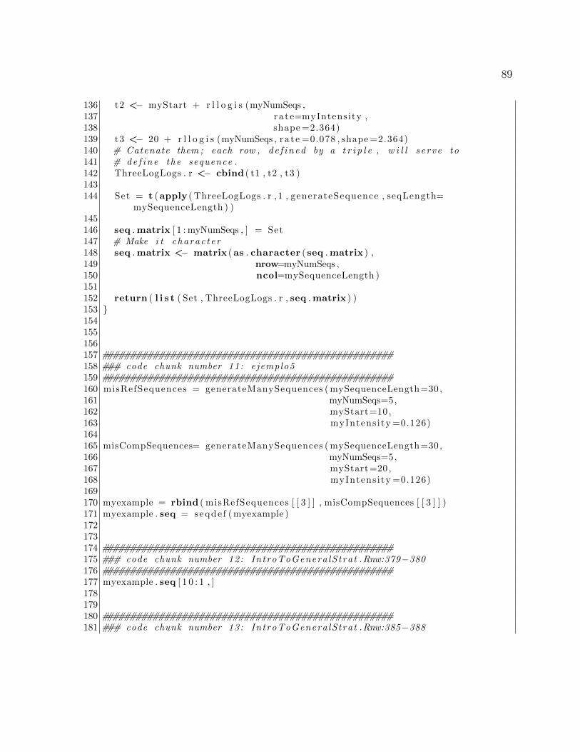
89
136 t2 <− myStart + r l l o g i s (myNumSeqs ,137 ra t e=myIntensity ,138 shape =2.364)139 t3 <− 20 + r l l o g i s (myNumSeqs , r a t e =0.078 , shape =2.364)140 # Catenate them ; each row , de f ined by a t r i p l e , w i l l s e r ve to141 # de f i n e the sequence .142 ThreeLogLogs . r <− cbind ( t1 , t2 , t3 )143144 Set = t (apply ( ThreeLogLogs . r , 1 , generateSequence , seqLength=
mySequenceLength ) )145146 seq . matrix [ 1 : myNumSeqs , ] = Set147 # Make i t charac t e r148 seq . matrix <− matrix ( as . character ( seq . matrix ) ,149 nrow=myNumSeqs ,150 ncol=mySequenceLength )151152 return ( l i s t ( Set , ThreeLogLogs . r , seq . matrix ) )153 }154155156157 ###################################################158 ### code chunk number 11: ejemplo5159 ###################################################160 misRefSequences = generateManySequences ( mySequenceLength=30,161 myNumSeqs=5,162 myStart=10,163 myIntens ity =0.126)164165 misCompSequences= generateManySequences ( mySequenceLength=30,166 myNumSeqs=5,167 myStart=20,168 myIntens ity =0.126)169170 myexample = rbind ( misRefSequences [ [ 3 ] ] , misCompSequences [ [ 3 ] ] )171 myexample . seq = seqde f ( myexample )172173174 ###################################################175 ### code chunk number 12: IntroToGenera lStrat .Rnw:379−380176 ###################################################177 myexample . seq [ 1 0 : 1 , ]178179180 ###################################################181 ### code chunk number 13: IntroToGenera lStrat .Rnw:385−388
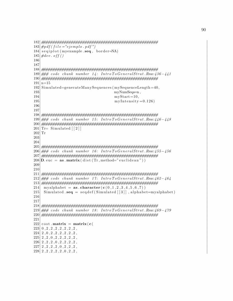
90
182 ###################################################183 #pdf ( f i l e =”ejemplo . pd f ”)184 s e q i p l o t ( myexample . seq , border=NA)185 #dev . o f f ( )186187188 ###################################################189 ### code chunk number 14: IntroToGenera lStrat .Rnw:436−441190 ###################################################191 n=15192 Simulated=generateManySequences ( mySequenceLength=40,193 myNumSeqs=n ,194 myStart=10,195 myIntens ity =0.126)196197198 ###################################################199 ### code chunk number 15: IntroToGenera lStrat .Rnw:446−448200 ###################################################201 Tr= Simulated [ [ 2 ] ]202 Tr203204205 ###################################################206 ### code chunk number 16: IntroToGenera lStrat .Rnw:455−456207 ###################################################208 D. euc = as . matrix ( d i s t (Tr , method=”euc l i d ean ”) )209210211 ###################################################212 ### code chunk number 17: IntroToGenera lStrat .Rnw:462−464213 ###################################################214 myalphabet = as . character (c ( 0 , 1 , 2 , 3 , 4 , 5 , 6 , 7 ) )215 Simulated . seq = seqde f ( Simulated [ [ 3 ] ] , a lphabet=myalphabet )216217218 ###################################################219 ### code chunk number 18: IntroToGenera lStrat .Rnw:469−479220 ###################################################221222 co s t . matrix = matrix (c (223 0 , 2 , 2 , 2 , 2 , 2 , 2 , 2 ,224 2 , 0 , 2 , 2 , 2 , 2 , 2 , 2 ,225 2 , 2 , 0 , 2 , 2 , 2 , 2 , 2 ,226 2 , 2 , 2 , 0 , 2 , 2 , 2 , 2 ,227 2 , 2 , 2 , 2 , 0 , 2 , 2 , 2 ,228 2 , 2 , 2 , 2 , 2 , 0 , 2 , 2 ,
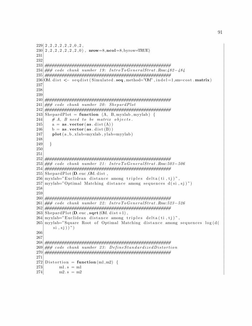
91
229 2 , 2 , 2 , 2 , 2 , 2 , 0 , 2 ,230 2 , 2 , 2 , 2 , 2 , 2 , 2 , 0 ) , nrow=8,ncol=8,byrow=TRUE)231232233 ###################################################234 ### code chunk number 19: IntroToGenera lStrat .Rnw:482−484235 ###################################################236 OM. d i s t <− s e q d i s t ( Simulated . seq , method=”OM” , i n d e l =1,sm=cos t .matrix )237238239240 ###################################################241 ### code chunk number 20: ShepardPlot242 ###################################################243 ShepardPlot = function (A, B, myxlab , myylab ) {244 # A, B need to be matrix o b j e c t s .245 a = as . vector ( as . d i s t (A) )246 b = as . vector ( as . d i s t (B) )247 plot ( a , b , xlab=myxlab , ylab=myylab )248249 }250251252 ###################################################253 ### code chunk number 21: IntroToGenera lStrat .Rnw:503−506254 ###################################################255 ShepardPlot (D. euc ,OM. d i s t ,256 myxlab=”Eucl idean d i s t ance among t r i p l e s d e l t a ( t i , t j ) ” ,257 myylab=”Optimal Matching d i s t anc e among sequences d( s i , s j ) ”)258259260 ###################################################261 ### code chunk number 22: IntroToGenera lStrat .Rnw:523−526262 ###################################################263 ShepardPlot (D. euc , sqrt (OM. d i s t +1) ,264 myxlab=”Eucl idean d i s t ance among t r i p l e s d e l t a ( t i , t j ) ” ,265 myylab=”Square Root o f Optimal Matching d i s t anc e among sequences l og (d(
s i , s j ) ) ”)266267268 ###################################################269 ### code chunk number 23: De f ineS tandard i z edDi s to r t i on270 ###################################################271272 D i s t o r t i o n = function (m1,m2) {273 m1. s = m1274 m2. s = m2
92
275 Numerator = sum( as . vector ( ( m1. s − m2. s ) ˆ2) )276 Denominator=sum( as . vector (m1. s ˆ2) )277 return ( sqrt ( Numerator/Denominator ) )278279 }280281 Cophenet icCorre l = function (m1,m2) {282 return ( cor ( as . vector (m1) , as . vector (m2) ) )283 }284285286287288 ###################################################289 ### code chunk number 24: GenerateOMandEucDistances1290 ###################################################291 numSequences=30292 runs = 1000293 a l l D i s t o r t = NULL294295 poss ib l eSeqLengths = seq ( from=35, to =55, by=5)296297 t o t a l n = runs*length ( pos s ib l eSeqLengths )298 I n t e r . T r i p l e s . d i s t = array (NA, c ( tota ln ,299 numSequences , numSequences ) )300 I n t e r . Seq .OM. d i s t = array (NA, c ( tota ln ,301 numSequences , numSequences ) )302303 LongitudSeq = rep (NA, t o t a l n )304 counter=0305306 # Let i s see what e f f e c t has the propor t ion between307 # replacement c o s t s and i n d e l c o s t s .308309 for ( th isSeqLength in pos s ib l eSeqLengths ) {310311312 for (myrun in 1 : runs ) {313314 counter=counter+1315 LongitudSeq [ counter ]= thisSeqLength316317 # crea t e t r i p l e s :318319 Simulated=generateManySequences (320 mySequenceLength=thisSeqLength ,321 myNumSeqs=numSequences ,

93
322 myStart=10, myIntens ity =0.126)323 T r i p l e s= Simulated [ [ 2 ] ]324 Sequences = Simulated [ [ 3 ] ]325326 # Ca lcu l a t e Eucl idean d i s t anc e s among t r i p l e s327 I n t e r . T r i p l e s . d i s t [ counter , , ] = as . matrix ( d i s t ( Tr ip l e s , method=”
euc l i d ean ”) )328329 # Create a ”se t−of−sequences ” o b j e c t330 Simulated . seq = seqde f ( Sequences , a lphabet=myalphabet )331332 # Ca lcu l a t e matrix o f i n t e r sequence OM d i s t an c e s f o r s e t333 # of sequences334 I n t e r . Seq .OM. d i s t [ counter , , ] <− s e q d i s t ( Simulated . seq , method=”OM” ,335 i n d e l =1,sm=cos t . matrix )336 }}337338339340 ###################################################341 ### code chunk number 25: Ca lcu la teDis tor t ionTrip lesOM1342 ###################################################343 D i s t o r t . Trip .OM = rep (NA, t o t a l n )344 Corr . Trip .OM = rep (NA, t o t a l n )345 counter=0346 for ( th isSeqLength in pos s ib l eSeqLengths ) {347 for (myrun in 1 : runs ) {348 counter=counter+1349350 # Ca lcu l a t e D i s t o r t i on between OM d i s t anc e s and Tr i p l e s d i s t an c e s .351 D i s t o r t . Trip .OM[ counter ] = D i s t o r t i o n ( I n t e r . Seq .OM. d i s t [ counter , , ] ,352 I n t e r . T r i p l e s . d i s t [ counter , , ] )353 Corr . Trip .OM[ counter ] = Cophenet icCorre l (354 I n t e r . Seq .OM. d i s t [ counter , , ] ,355 I n t e r . T r i p l e s . d i s t [ counter , , ] )356357358 } }359360361 ###################################################362 ### code chunk number 26: ShepPlotTripOM1363 ###################################################364 boxplot ( D i s t o r t . Trip .OM ˜ LongitudSeq ,365 log=”y ” ,366 xlab=”Sequence Length ” ,367 ylab=”Measure o f D i s t o r t i o n ”)

94
368369370 ###################################################371 ### code chunk number 27: ShepPlotTripOM2372 ###################################################373 boxplot ( Corr . Trip .OM ˜ LongitudSeq ,374 xlab=”Sequence Length ” ,375 ylab=”Measure o f Co r r e l a t i on ”)376377378 ###################################################379 ### code chunk number 28: Generate4245WithLength40380 ###################################################381 generateSequence ( t r i p l e=c (15 ,42 ,30 ) , seqLength =40)382 generateSequence ( t r i p l e=c (15 ,45 ,30 ) , seqLength =40)383384385 ###################################################386 ### code chunk number 29: Generate4245WithLength48387 ###################################################388 generateSequence ( t r i p l e=c (15 ,42 ,30 ) , seqLength =50)389 generateSequence ( t r i p l e=c (15 ,45 ,30 ) , seqLength =50)390391392 ###################################################393 ### code chunk number 30: Def ineCostMatrix394 ###################################################395396 co s t . matrix = matrix (c (397 0 , 2 , 2 , 2 , 2 , 2 , 2 , 2 ,398 2 , 0 , 2 , 2 , 2 , 2 , 2 , 2 ,399 2 , 2 , 0 , 2 , 2 , 2 , 2 , 2 ,400 2 , 2 , 2 , 0 , 2 , 2 , 2 , 2 ,401 2 , 2 , 2 , 2 , 0 , 2 , 2 , 2 ,402 2 , 2 , 2 , 2 , 2 , 0 , 2 , 2 ,403 2 , 2 , 2 , 2 , 2 , 2 , 0 , 2 ,404 2 , 2 , 2 , 2 , 2 , 2 , 2 , 0 ) , nrow=8,ncol=8,byrow=TRUE)405406407 ###################################################408 ### code chunk number 31: GenerateOMandEucDistances409 ###################################################410 numSequences=30411 runs = 1000412 a l l D i s t o r t = NULL413414 p o s s i b l e c o s t s = seq ( from =0.25 , to =3, length . out=12)

95
415416 t o t a l n = runs*length ( p o s s i b l e c o s t s )417418 Inde lCost = rep (NA, t o t a l n )419420 I n t e r . T r i p l e s . d i s t = array (NA, c ( tota ln ,421 numSequences , numSequences ) )422 I n t e r . Seq .OM. d i s t = array (NA, c ( tota ln ,423 numSequences , numSequences ) )424425 counter=0426427 # Let i s see what e f f e c t has the propor t ion between428 # replacement c o s t s and i n d e l c o s t s .429430 for ( i n d e l c o s t in p o s s i b l e c o s t s ) {431432 for (myrun in 1 : runs ) {433434 counter=counter+1435 Inde lCost [ counter ]= i n d e l c o s t436437 # crea t e t r i p l e s :438439 Simulated=generateManySequences (440 mySequenceLength=30,441 myNumSeqs=numSequences ,442 myStart=10, myIntens ity =0.126)443 T r i p l e s= Simulated [ [ 2 ] ]444 Sequences = Simulated [ [ 3 ] ]445446 # Ca lcu l a t e Eucl idean d i s t anc e s among t r i p l e s447 I n t e r . T r i p l e s . d i s t [ counter , , ] = as . matrix ( d i s t ( Tr ip l e s , method=”
euc l i d ean ”) )448449 # Create a ”se t−of−sequences ” o b j e c t450 Simulated . seq = seqde f ( Sequences , a lphabet=myalphabet )451452 # Ca lcu l a t e matrix o f i n t e r sequence OM d i s t an c e s f o r s e t453 # of sequences454 I n t e r . Seq .OM. d i s t [ counter , , ] <− s e q d i s t ( Simulated . seq , method=”OM” ,455 i n d e l=i n d e l c o s t , sm=cos t . matrix )456 }}457458459460 ###################################################

96
461 ### code chunk number 32: Ca lcu la teDis tor t ionTrip l e sOM462 ###################################################463 D i s t o r t . Trip .OM = rep (NA, t o t a l n )464 counter=0465 for ( i n d e l c o s t in p o s s i b l e c o s t s ) {466 for (myrun in 1 : runs ) {467 counter=counter+1468469 # Ca lcu l a t e d i s t o r t i o n between OM d i s t an c e s and Tr i p l e s d i s t an c e s .470 D i s t o r t . Trip .OM[ counter ] = D i s t o r t i o n ( I n t e r . Seq .OM. d i s t [ counter , , ] ,471 I n t e r . T r i p l e s . d i s t [ counter , , ] )472473 } }474475476 ###################################################477 ### code chunk number 33: ShepPlotTripOM478 ###################################################479 boxplot ( D i s t o r t . Trip .OM ˜ IndelCost ,480 log=”y ” ,481 xlab=”Cost o f I n s e r t i o n−Dele t ion ” ,482 ylab=”Measure o f D i s t o r t i o n ”)483484485 ###################################################486 ### code chunk number 34: FindNonEuclidean487 ###################################################488 # ade4 package prov ide s i s . e u c l i d489 l ibrary ( ade4 )490491 I sEuc l idean = rep (NA, runs*length ( p o s s i b l e c o s t s ) )492 counter=0493494 for ( i n d e l c o s t in p o s s i b l e c o s t s ) {495496 for ( j in 1 : runs ) {497498 counter=counter+1499500 # Determine i f matrix i s Eucl idean or not .501 # i s . e u c l i d e xpec t s a d i s t ob j e c t , so i t shou ld be502 # transformed f i r s t ( take square root , and make503 # di s t ance o b j e c t ) .504 I sEuc l idean [ counter ] = i s . e u c l i d (505 as . d i s t (506 sqrt ( I n t e r . Seq .OM. d i s t [ counter , , ] ) ) )507 }
97
508 }509 EucByIndel = aggregate ( I sEuc l idean , by=l i s t ( Inde lCost ) , mean)510511512513 ###################################################514 ### code chunk number 35: PlotEuc515 ###################################################516 plot ( EucByIndel [ [ 1 ] ] , EucByIndel [ [ 2 ] ] ,517 xlab=”Inde l c o s t s ” ,518 ylab=paste ( ”Proport ion o f Eucl idean matr i ce s ”) )519520521 ###################################################522 ### code chunk number 36: MDSDeepPrep523 ###################################################524 D i s t o r t . d i f f = rep (NA, t o t a l n )525 #dim( In t e r . Seq .OM. d i s t )526 #to t a l n527 #In t e r . Seq .OM. d i s t [ 1 , , ]528 #counter529530531 ###################################################532 ### code chunk number 37: MDSDeep533 ###################################################534 l ibrary ( vegan )535 counter=0536 for ( i n d e l c o s t in p o s s i b l e c o s t s ) {537538 for ( j in 1 : runs ) {539540 counter=counter+1541542 # Get a MDS rep r e s en t a t i on from OM matr ices .543 MDS. coord = metaMDS( I n t e r . Seq .OM. d i s t [ counter , , ] ,544 distance=”euc l i d ean ” , k=3)$points545 MDS. d i s t = as . matrix ( d i s t (MDS. coord ) )546 # Ca lcu l a t e d i s t o r t i o n between matrix o f t rue in t e r−t r i p l e547 # di s t anc e s and d i s t ance matrix from MDS so l u t i o n .548 D i s t o r t i o n . True .MDS = D i s t o r t i o n (MDS. d i s t ,549 I n t e r . T r i p l e s . d i s t [ counter , , ] )550 #Corre l . True .MDS = Cophenet icCorre l (MDS. d i s t ,551 # In t e r . Tr i p l e s . d i s t [ counter , , ] )552 # We a l ready c a l c u l a t e d d i s t o r t i o n between553 # true in t e r−t r i p l e d i s t an c e s and OM; i t i s D i s t o r t . Trip .OM554 # Is t h i s d i s t o r t i o n

98
555556 D i s t o r t i o n . d i f f [ counter ] = D i s t o r t i o n . True .MDS − Dis to r t . Trip .OM[
counter ]557 }558 }559 #summary( D i s t o r t i on . d i f f )560561 # Ca lcu l a t e an MDS so l u t i o n to OM d i s t anc e s and ge t a562 # new matrix o f d i s t an c e s from i t .563 #mds . coord <− cmdscale ( In t e r . Seq .OM. d i s t , k=3)564 #mds . coord <− ( isoMDS( as . d i s t ( In t e r . Seq .OM. d i s t ) , k=3, p=2))$po in t s565 #In t e r .MDS.OM. d i s t <− as . matrix ( d i s t (mds . coord ) )566567 # Ca lcu l a t e d i s t o r t i o n between matrix o f in t e r−t r i p l e d i s t an c e s568 # and matrix o f MDS so l u t i o n to OM d i s t anc e s .569 #Dis t o r t . Trip .MDS.om[ counter ] = Di s t o r t i on ( In t e r .MDS.OM. d i s t ,570 # In t e r . Tr i p l e s . d i s t )571572 #Dis t o r t .OM.MDS[ counter ] = Di s t o r t i on ( In t e r .MDS.OM. d i s t , I n t e r . Seq .OM
. d i s t )573574575576 ###################################################577 ### code chunk number 38: IntroToGenera lStrat .Rnw:1181−1182578 ###################################################579 D i s t o r t i o n . d i f f [ D i s t o r t i o n . d i f f > 10 ] <− NA580581582 ###################################################583 ### code chunk number 39: IntroToGenera lStrat .Rnw:1185−1186584 ###################################################585 summary( D i s t o r t i o n . d i f f )586587588 ###################################################589 ### code chunk number 40: D i s t o r t d i f f590 ###################################################591 boxplot ( D i s t o r t i o n . d i f f ˜ IndelCost ,592 xlab=”Cost o f I n s e r t i o n−Dele t ion ” ,593 ylab=”D i s t o r t i o n d i f f e r e n c e ”)594595596 ###################################################597 ### code chunk number 41: GenerOM598 ###################################################599 n=100
99
600 Simulated=generateManySequences (myNumSeqs=n ,601 mySequenceLength=40,602 myStart=10,603 myIntens ity =0.126)604 ####################################605 # True t r i p l e s606 T r i p l e s= Simulated [ [ 2 ] ]607 # Ca lcu l a t e t rue Eucl idean d i s t anc e s among t r i p l e s608 I n t e r . T r i p l e s . d i s t = as . matrix ( d i s t ( Tr ip l e s , method=”euc l i d ean ”) )609610 ####################################611 # ca l c u l a t i o n o f OM d i s t anc e s612 myalphabet = as . character (c ( 0 , 1 , 2 , 3 , 4 , 5 , 6 , 7 ) )613 Simulated . seq = seqde f ( Simulated [ [ 3 ] ] , a lphabet=myalphabet )614615 co s t . matrix = matrix (c (616 0 , 2 , 2 , 2 , 2 , 2 , 2 , 2 ,617 2 , 0 , 2 , 2 , 2 , 2 , 2 , 2 ,618 2 , 2 , 0 , 2 , 2 , 2 , 2 , 2 ,619 2 , 2 , 2 , 0 , 2 , 2 , 2 , 2 ,620 2 , 2 , 2 , 2 , 0 , 2 , 2 , 2 ,621 2 , 2 , 2 , 2 , 2 , 0 , 2 , 2 ,622 2 , 2 , 2 , 2 , 2 , 2 , 0 , 2 ,623 2 , 2 , 2 , 2 , 2 , 2 , 2 , 0 ) , nrow=8,ncol=8,byrow=TRUE)624 Simulated . d i s t <− s e q d i s t ( Simulated . seq , method=”OM” , i n d e l =1,sm=cos t .
matrix )625626627628629 ###################################################630 ### code chunk number 42: IntroToGenera lStrat .Rnw:1268−1270631 ###################################################632 hist ( as . vector ( as . d i s t ( I n t e r . T r i p l e s . d i s t ) ) , xl im=c (0 ,100) ,633 xlab=”Inte r i t em d i s t a n c e s between l a t e n t t r i p l e s ”)634635636 ###################################################637 ### code chunk number 43: IntroToGenera lStrat .Rnw:1282−1283638 ###################################################639 hist ( as . d i s t ( Simulated . d i s t ) , x lab=”Inte r i t em d i s t a n c e s ” , main=”OM
d i s t a n c e s ”)640641642 ###################################################643 ### code chunk number 44: getmds644 ###################################################
100
645 MDS. coord = metaMDS( Simulated . d i s t ,646 distance=”euc l i d ean ” , k=3)$points647 MDS. d i s t = as . matrix ( d i s t (MDS. coord ) )648649650 ###################################################651 ### code chunk number 45: IntroToGenera lStrat .Rnw:1302−1303652 ###################################################653 hist ( as . d i s t (MDS. d i s t ) , main=”MDS s o l u t i o n ” , xlab=”Inte r i t em d i s t a n c e s ”)654655656 ###################################################657 ### code chunk number 46: IntroToGenera lStrat .Rnw:1334−1347658 ###################################################659 l ibrary (MASS) # prov ide s mvrnorm()660661 # Diagonal Variance/Covariance matrix662663 p=3664 mySigma=matrix (c665 (1 , 0 , 0 ,666 0 ,1 ,0 ,667 0 ,0 ,1 ) ,p , p )668669 X = mvrnorm (100 ,mu=rep (0 , p ) , Sigma=mySigma)670 d = d i s t (X)671 d2 = d i s t (X) ˆ2 # Get the square o f such d i s t an c e s672673674 ###################################################675 ### code chunk number 47: IntroToGenera lStrat .Rnw:1353−1354676 ###################################################677 hist (d , f r e q=FALSE, xlab=”Inte r i t em d i s tance s , i tems are Multinormal ”)678679680 ###################################################681 ### code chunk number 48: IntroToGenera lStrat .Rnw:1526−1530682 ###################################################683 vec1 = c ( rep ( 0 , 5 ) , rep ( 1 , 5 ) )684 d i f f e r e n c e s .matrix = 1 * outer ( vec1 , vec1 ,FUN= ”==”)685 d i f f e r e n c e s .matrix . a s d i s t = as . d i s t ( d i f f e r e n c e s . matrix )686687688689 ###################################################690 ### code chunk number 49: IntroToGenera lStrat .Rnw:1544−1547691 ###################################################

101
692 vec1693 X = 1 * outer ( vec1 , vec1 ,FUN=” !=”)694 X695696697 ###################################################698 ### code chunk number 50: IntroToGenera lStrat .Rnw:1550−1552699 ###################################################700 X * d . example701 sum(X * d . example)/2 # usua l l y sum over lower t r i a n g l e702703704 ###################################################705 ### code chunk number 51: IntroToGenera lStrat .Rnw:1559−1563706 ###################################################707 X = 1*outer ( vec1 , vec1 ,FUN=”==”)708 X709 X * d . example710 sum(X * d . example)/2711712713 ###################################################714 ### code chunk number 52: IntroToGenera lStrat .Rnw:1576−1579715 ###################################################716 vec1717 permuted . vector = sample ( vec1 , replace=FALSE)718 permuted . vector719720721 ###################################################722 ### code chunk number 53: IntroToGenera lStrat .Rnw:1582−1586723 ###################################################724 X = 1*outer ( permuted . vector , permuted . vector ,FUN=”==”)725 X726 X * d . example727 sum(X * d . example)/2728729730 ###################################################731 ### code chunk number 54: FreeMemByDeletingHugeMatrices732 ###################################################733 rm( I n t e r . T r i p l e s . d i s t )734 rm( I n t e r . Seq .OM. d i s t )
./IntroToGeneralStrat.R
1 ### R code from v i g n e t t e source ' s imu la t i on .Rnw'

102
23 ###################################################4 ### code chunk number 1 : somevars5 ###################################################6 TotalReps=20007 theta =0.58 SequencesPerSet = 309 SetsSequencesRe fe rence= SequencesPerSet* theta
10 SetsSequencesSecondGroup= SequencesPerSet*(1− theta )11 NumberOfSteps=10121314 ###################################################15 ### code chunk number 2 : i n i t16 ###################################################1718 # For p a r a l l e l coding19 l ibrary (doMC)20 registerDoMC ( )21 #getDoParWorkers ( )2223 #i = 1: SequenceLength242526 ###################################################27 ### code chunk number 3 : s imu la t i on .Rnw:103−10728 ###################################################29 vec1 = c ( rep (0 , Set sSequencesRe fe rence ) ,30 rep (1 , SetsSequencesSecondGroup ) )31 d i f f e r e n c e s . matrix = 1 * outer ( vec1 , vec1 ,FUN= ”==”)32 d i f f e r e n c e s . matrix . a s d i s t = as . d i s t ( d i f f e r e n c e s . matrix )333435 ###################################################36 ### code chunk number 4 : s imu la t i on .Rnw:111−12737 ###################################################38 Tot0 = rep (0 , TotalReps )39 p . va lue s . Mantel <− Tot040 p . va lue s . AndersonF <− Tot041 p . va lue s .ANOSIM <− Tot042 p . va lue s . mrpp <− Tot043 p . va lue s . t t e s t <− Tot044 p . va lue s . perm .median <− Tot04546 p . va lue s .MANOVA. pcoa <− Tot047 p . va lue s . Mantel . pcoa <− Tot048 p . va lue s . Anderson . pcoa <− NULL

103
49 p . va lue s .ANOSIM. pcoa <− NULL50 p . va lue s . mrpp . pcoa <− NULL515253545556 ###################################################57 ### code chunk number 5 : subsMatr ix58 ###################################################59 co s t . matrix = matrix (c (60 0 , 2 , 2 , 2 , 2 , 2 , 2 , 2 ,61 2 , 0 , 2 , 2 , 2 , 2 , 2 , 2 ,62 2 , 2 , 0 , 2 , 2 , 2 , 2 , 2 ,63 2 , 2 , 2 , 0 , 2 , 2 , 2 , 2 ,64 2 , 2 , 2 , 2 , 0 , 2 , 2 , 2 ,65 2 , 2 , 2 , 2 , 2 , 0 , 2 , 2 ,66 2 , 2 , 2 , 2 , 2 , 2 , 0 , 2 ,67 2 , 2 , 2 , 2 , 2 , 2 , 2 , 0 ) , nrow=8,ncol=8,byrow=TRUE)686970 ###################################################71 ### code chunk number 6 : showCosts72 ###################################################73 co s t . matrix747576 ###################################################77 ### code chunk number 7 : subsMatr ix . NonMetric78 ###################################################79 co s t . matrix . nonMetric = matrix (c (80 0 , 1 , 1 , 1 , 1 , 1 , 1 , 1 ,81 1 , 0 , 1 , 1 , 1 , 1 , 1 , 1 ,82 1 , 1 , 0 , 1 , 1 , 1 , 1 , 1 ,83 1 , 1 , 1 , 0 , 1 , 1 , 1 , 1 ,84 1 , 1 , 1 , 1 , 0 , 1 , 1 , 1 ,85 1 , 1 , 1 , 1 , 1 , 0 , 1 , 1 ,86 1 , 1 , 1 , 1 , 1 , 1 , 0 , 1 ,87 1 , 1 , 1 , 1 , 1 , 1 , 1 , 0 ) , nrow=8,ncol=8,byrow=TRUE)888990 ###################################################91 ### code chunk number 8 : coreOfSim92 ###################################################93 l ibrary ( vegan )94 l ibrary ( ape )95 l ibrary ( e c o d i s t )

104
96 l ibrary ( actuar )97 l ibrary (TraMineR)9899 SimulateSequences <− function ( SequenceLength ,
100 Re f e r ence In t en s i ty ,101 Start2 ,102 mylambda2 ) {103104 seq . matrix=NULL105 seq . matrix=matrix (nrow=SequencesPerSet , ncol=SequenceLength )106107 for ( kounter in 1 : TotalReps ) {108109 ReferenceSet = generateManySequences (110 mySequenceLength=SequenceLength ,111 myNumSeqs=SetsSequencesReference ,112 myStart=10,113 myIntens ity=R e f e r e n c e I n t e n s i t y )114115 t2 . b a s e l i n e = ReferenceSet [ [ 2 ] ] [ , 2 ]116117 ComparativeSet = generateManySequences (118 mySequenceLength=SequenceLength ,119 myNumSeqs=SetsSequencesSecondGroup ,120 myStart=Start2 ,121 myIntens ity=mylambda2 )122123 t2 . comp = ComparativeSet [ [ 2 ] ] [ , 2 ]124125 seq . matrix = rbind ( Re fe renceSet [ [ 3 ] ] , ComparativeSet [ [ 3 ] ] )126127 ###################################################################128 # For our more parametr ic exp l o ra t i on , l e t us d e r i v e a d i s c r e t i z e d129 # trans format ion o f the random quan t i t y o f i n t e r e s t :130131 #t2 . b a s e l i n e = ob j e c t [ [ 3 ] ]132 #t2 . comp = ob j e c t [ [ 4 ] ]133134 x . b a s e l i n e = cei l ing ( t2 . b a s e l i n e )135 x . b a s e l i n e . trunc = subset ( x . ba s e l i n e , ( x . b a s e l i n e <= SequenceLength )
)136 x . tocompare = cei l ing ( t2 . comp)137 x . tocompare . trunc = subset ( x . tocompare , ( x . tocompare <=
SequenceLength ) )138 # Truncated v e r s i on s correspond to those cases where139 # t was g r ea t e r than 41.140
105
141142143 # Now tha t we have a s e t o f sequences s t o r ed in seq . matrix ,144 # produce a d i s t ance matrix from sequences us ing an OM di s t ance145 # and s t o r e i t in matd i s t .146 myalphabet = as . character (c ( 0 , 1 , 2 , 3 , 4 , 5 , 6 , 7 ) )147 matseq <− s eqde f ( seq .matrix , a lphabet=myalphabet )148 matdist <− s e q d i s t ( matseq , method=”OM” , i n d e l =1,sm=cos t .matrix )149150 #matd is t . nonmetric <−s e q d i s t (matseq , method=”OM”, i n d e l =1,sm=cos t .
matrix . nonMetric )151152 # This i s the par t where , g i ven two matrices ,153 # the t e s t s are run .154 ###########################################################155 # Mantel c o r r e l a t i o n between matd i s t (Y) and the matrix o f156 # or i g i n s ( f i r s t h a l f o f peop l e are f i x ed−parameter peop l e157 my. mantel = e c o d i s t : : mantel ( d i f f e r e n c e s . matrix . a s d i s t158 ˜ as . d i s t ( matdist ) ,159 nperm=1000)160 # t h i s v ec t o r o f s i z e TotalReps s t o r e s the p−va l u e s f o r each161 # r e p e t i t i o n .162 # one−t a i l e d p−va lue (H0 : r > = 0)163 p . va lue s . Mantel [ kounter ] = my. mantel [ 3 ]164 ######################################################165 # d i s s a s s o c McArdle and Anderson166 my. d i s s a s s o c = d i s s a s s o c ( matdist , group=vec1 ,R=1000)167 p . va lue s . AndersonF [ kounter ] = my. d i s s a s s o c$stat [ 1 , 2 ]168 #####################################################169 # MRPP ?170 my. mrpp = mrpp( dat=as . d i s t ( matdist ) ,171 grouping=vec1 ,172 permutations =1000)173 p . va lue s . mrpp [ kounter ] = my. mrpp$Pvalue174 #p . va l u e s .mrpp [ kounter ] = NA175 #############################################176 # forc e random matrix to a PCoA form ,177 matdist . pcoa <− ( pcoa ( matdist ) )$ve c to r s178179 # now , wi th a matrix o f coord ina t e s I can do many t h i n g s .180 # One i s to assume tha t such matrix i s mul t inormal ly181 # d i s t r i b u t e d , and run a t e s t . matd i s t . pcoa .m182 manovafit <− summary(manova( matdist . pcoa ˜ vec1 ) )183 p . va lue s .MANOVA. pcoa [ kounter ] = manovafit$ s t a t s [ ”vec1 ” , ”Pr(>F) ” ]184185186 ################################################
106
187 # This one in s t ead take s the pcoa , conver t s i t back188 # to a matrix o f d i s t an c e s (meaning i t ”c l eans ” the non189 # euc l i d i an weirdness , and reruns the Mantel t e s t s on i t .190 matdist . pcoa .m <− d i s t ( matdist . pcoa )191192 my. mantel . pcoa = e c o d i s t : : mantel ( d i f f e r e n c e s . matrix . a s d i s t193 ˜ matdist . pcoa .m, nperm=1000)194 p . va lue s . Mantel . pcoa [ kounter ] = my. mantel . pcoa [ 3 ]195196 ###############################################197 #198 # Take squared roo t o f matrix199200 matdist . r a i s e d <− matdist ˆ ( 0 . 5 )201202203 ########################################################204 # More parametr ic t e s t s :205 # Plain comparison o f two sample means :206207 p . va lue s . t t e s t [ kounter ] = t . t e s t ( x . b a s e l i n e . trunc , x . tocompare . trunc
)$p . va lue208 ########################################################209 # permuta t iona l t e s t o f d i f f e r e n c e s between medians .210 #211 d i f f . medians = abs (median( x . b a s e l i n e ) − median( x . tocompare ) )212 d i f f . vector = rep (0 ,1000)213 x . a l l = c ( x . ba s e l i n e , x . tocompare )214 i n d i c a t o r = c ( rep (0 , Set sSequencesRe fe rence ) , rep (1 ,
SetsSequencesSecondGroup ) )215 for ( j in 1 :1000) {216 perm . i n d i c a t o r = sample ( i nd i ca to r , replace=FALSE)217 median1 = median( x . a l l [ perm . i n d i c a t o r ==1])218 median0 = median( x . a l l [ perm . i n d i c a t o r ==0])219 d i f f . vector [ j ]=abs ( median1−median0 )220 }221 p . va lue s . perm .median [ kounter ] = sum( d i f f . vector >= d i f f . medians )/
1000222 #############################################################223 }224 # Function re turns the propor t ion o f t e s t p−va l u e s225 # whose va l u e s i n d i c a t e a r e j e c t i o n o f Nul l Hypothes i s .226 myvector=c ( Start2 ,227 mylambda2 ,228 sum(p . va lue s . Mantel < 0 . 0 5 )/TotalReps ,229 sum(p . va lue s . AndersonF < 0 . 0 5 )/TotalReps ,230 sum(p . va lue s . mrpp < 0 . 0 5 )/TotalReps ,

107
231 sum(p . va lue s . t t e s t < 0 . 0 5 )/TotalReps ,232 sum(p . va lue s . perm .median < 0 . 0 5 )/TotalReps ,233 sum(p . va lue s .MANOVA. pcoa < 0 . 0 5 )/TotalReps ,234 sum(p . va lue s . Mantel . pcoa < 0 . 0 5 )/TotalReps ,235 SequenceLength236 )237 #gr i d . r e s u l t s = rb ind ( g r i d . r e s u l t s , myvector )238239 #return ( g r i d . r e s u l t s )240 return ( myvector )241 }242243244 ###################################################245 ### code chunk number 9 : s imul246 ###################################################247 data . sim . mll = NULL248 PassSequenceLength=40249 range . a2 = seq ( from=10, to =15, length . out=10)250251 va lues <− f o r each ( f a . second = range . a2 ,252 . combine=rbind ) %dopar% {SimulateSequences (253 SequenceLength=PassSequenceLength ,254 R e f e r e n c e I n t e n s i t y =0.126 ,255 Star t2=fa . second ,256 mylambda2=0.126)}257258 data . sim . mll = va lues259 #va lue s = NULL260261262 ###################################################263 ### code chunk number 10: g ra f264 ###################################################265 powerplot = function ( mydata , xlegend , cua l ) {266267 i f ( cua l==1) {minx=10}268 i f ( cua l==2) {minx=0.078}269 i f ( cua l==10) {minx=25}270271 x = mydata [ , cua l ]272273 pMantel=mydata [ , 3 ]274 pPermanova=mydata [ , 4 ]275 pMRPP=mydata [ , 5 ]276 pt . trunc=mydata [ , 6 ]277 pd i f fmed ians=mydata [ , 7 ]

108
278 pmanova . pcoa=mydata [ , 8 ]279 pmantel . pcoa=mydata [ , 9 ]280281282283 plot (x , pMantel , pch=”M” , type=”b” , col=”green ” ,284 xlab=xlegend , ylab=”% of p−va lues < . 05 ” , yl im=c ( 0 : 1 ) )285 points (x , pPermanova , pch=”P” , type=”b” , col=”purple ”)286 points (x ,pMRPP, pch=”*” , type=”b” , col=”blue ”)287 points (x , pt . trunc , pch=”t ” , type=”b” , col=”brown ”)288 points (x , pdi f fmedians , pch=”+” , type=”b” , col=”red ”)289 points (x , pmanova . pcoa , pch=”m” , type=”b” , col=”black ”)290 #po in t s (mydata [ , cua l ] , mydata$mantel . pcoa , pch=”x ” , type=”b ” , c o l=”b l ue ”)291 #po in t s (mydata [ , cua l ] , mydata [ , 1 0 ] , pch=”z ” , type=”b ” , c o l=”dark b l u e ”)292293 legend ( minx , 1 , c ( ”Mantel ” , ”Permanova ” , ”MRPP” , ”t truncated ” , ” d i f f
medians ” ,294 ”MANOVA on PCoA”) ,295 pch=c ( ”M” , ”P” , ”*” , ”t ” , ”+” , ”m”) ,296 col=c ( ”green ” , ”purple ” , ”blue ” , ”brown ” , ”red ” , ”black ”) ,297 l t y =1)298 }299300301 ###################################################302 ### code chunk number 11: s imu la t i on .Rnw:412−414303 ###################################################304 #data . sim . ml l305 powerplot (data . sim . mll , ”Sta r t parameter ” ,1 )306307308 ###################################################309 ### code chunk number 12: s imu l In t ens310 ###################################################311 data . sim . mll = NULL312 PassSequenceLength=40313 range . lambda2 = seq ( from =0.078 , to =0.205 , length . out=10)314315 va lues <− f o r each ( lambda2 = range . lambda2 ,316 . combine=rbind ) %dopar% {317 SimulateSequences (318 SequenceLength=PassSequenceLength ,319 R e f e r e n c e I n t e n s i t y =0.078 ,320 Star t2 =10,321 mylambda2=lambda2 )322 }323

109
324 va lues325326 #for (my. lambda . second in range . lambda2 ) {327 # va lue s = SimulateSequences (a . second=10, lambda . second=my. lambda . second
)328329 #data . sim . ml l = rb ind ( data . sim . mll , v a l u e s )330 # }331332333 ###################################################334 ### code chunk number 13: s imu la t i on .Rnw:497−498335 ###################################################336 #data . sim . ml l337338339 ###################################################340 ### code chunk number 14: g ra f3341 ###################################################342 powerplot ( values , ”Rate parameter ” ,2 )
./simulation.R
1 ### R code from v i g n e t t e source ' Ef fec tOfLength .Rnw'
23 ###################################################4 ### code chunk number 1 : E f f e c tLeng th5 ###################################################6 #va lue s = NULL7 #data . sim . ml l = NULL8 range . s eq l ength = c (25 , 40 , 50 , 60)9
10 va lue s <− f o r each ( thisPassSequenceLength = range . s eq length ,11 . combine=rbind ) %dopar% {12 SimulateSequences (13 SequenceLength=thisPassSequenceLength
,14 R e f e r e n c e I n t e n s i t y =0.126 ,15 Star t2 =15,16 mylambda2=0.126)17 }18192021 ###################################################22 ### code chunk number 2 : Ef fec tOfLength .Rnw:31−3323 ###################################################
110
24 powerplot ( values , ”Sequence Length ” ,10)25 va lue s=NULL262728 ###################################################29 ### code chunk number 3 : newsim30 ###################################################31 generateManySequences <− function ( mySequenceLength ,32 myNumSeqs ,33 myStart ,34 myIntens ity ) {3536 seq . matrix=NULL37 seq . matrix=matrix (nrow=myNumSeqs , ncol=mySequenceLength )3839 #################################################################40 # Fi r s t genera te t h r ee v e c t o r s o f L o g l o g i s t random quan t i t i e s ,41 # each with l en g t h Set sSequencesReferences .42 t1 <− 0 + rtrunc (n=myNumSeqs , spec=” l l o g i s ” ,43 a=0,b=mySequenceLength ,44 ra t e =0.078 , shape =2.364)4546 t2 <− myStart + rtrunc (n=myNumSeqs , spec=” l l o g i s ” ,47 a=0, b=mySequenceLength ,48 ra t e=myIntensity , shape =2.364)4950 t3 <− 20 + rtrunc (n=myNumSeqs , spec=” l l o g i s ” ,51 a=0,b=mySequenceLength ,52 ra t e =0.078 , shape =2.364)5354 # Catenate them ; each row , de f ined by a t r i p l e , w i l l s e r ve to55 # de f i n e the sequence .56 ThreeLogLogs . r <− cbind ( t1 , t2 , t3 )5758 Set = t (apply ( ThreeLogLogs . r , 1 , generateSequence , seqLength=
mySequenceLength ) )5960 seq . matrix [ 1 : myNumSeqs , ] = Set61 # Make i t charac t e r62 seq . matrix <− matrix ( as . character ( seq . matrix ) ,63 nrow=myNumSeqs ,64 ncol=mySequenceLength )6566 return ( l i s t ( Set , ThreeLogLogs . r , seq . matrix ) )67 }6869

111
7071 ###################################################72 ### code chunk number 4 : E f f ec tLeng th273 ###################################################74 l ibrary ( t r u n c d i s t )75 va lue s = NULL76 #data . sim . ml l = NULL77 range . s eq l ength = c (25 , 40 , 50 , 60)7879 va lues <− f o r each ( thisPassSequenceLength = range . s eq length ,80 . combine=rbind ) %dopar% {81 SimulateSequences (82 SequenceLength=thisPassSequenceLength
,83 R e f e r e n c e I n t e n s i t y =0.126 ,84 Star t2 =15,85 mylambda2=0.126)86 }87888990 ###################################################91 ### code chunk number 5 : Ef fec tOfLength .Rnw:114−11592 ###################################################93 powerplot ( values , ”Sequence Length ” ,10)
./EffectOfLength.R