optimal protocol for polarization ququart state … · optimal protocol for polarization ququart...

Applied Mathematics & Information Sciences 3(1) (2009), 1–12– An International Journalc©2009 Dixie W Publishing Corporation, U. S. A.

Optimal Protocol for Polarization Ququart State Tomography

E. V. Moreva1, Yu. I. Bogdanov2, A. K. Gavrichenko2, I. V. Tikhonov3, and S. P. Kulik3

1Moscow Engineering Physics Institute (State University)

Email Address: [email protected] of Physics and Technology, Russian Academy of Science

3Faculty of Physics, Moscow State University, 119992, Moscow, Russia

Received July 23, 2008; Revised October 14, 2008

We develop a practical quantum tomography protocol and implement measurementsof pure states of ququarts realized with polarization states of photon pairs (biphotons).The method is based on an optimal choice of the measuring scheme’s parameters thatprovides better quality of reconstruction for the fixed set of statistical data. A highaccuracy of the state reconstruction (above 0.99) indicates that developed methodologyis adequate.

Keywords: Quantum tomography, biphotons, polarization ququart.

1 Introduction.

For the last several years many elegant experiments were performed in which differentkinds of multi-dimensional quantum states (qudits) were introduced [17–21, 23–26] (formore details see the review [11]). Most of them are based on the states of light emittedvia spontaneous parametric down-conversion (SPDC). In this process photons of the laserpump decay on the pairs of photons (biphotons) inside the crystal possessing non-zeroquadratic susceptibility. In stationary case the sum of daughter photons frequencies coin-cides with the frequency of the pump ws + wi = wp and intensity of the biphoton lightemitted from the crystal is maximal when phase matching condition ks + ki = kp holds.Choosing particular regime of SPDC one can prepare a whole family of the biphoton stateswith different properties. In this paper we focus upon polarization states of biphotons al-though some other qudits can be realized with photon pairs. Selecting so called frequencydegenerate (ws = wi) and collinear (ks||ki) regime of SPDC, polarization qutrits (d = 3)can be realized. Preparation of arbitrary polarization qutrit (d = 3) was reported in [6]. Theexperimental method for engineering with pure states of ququarts (d = 4) was presentedin [9, 10].

2 E. V. Moreva et al.

Quality assurance of preparation and transformation requires a complete characteriza-tion of these states, which can be accomplished through a procedure known as quantumprocess tomography. The first protocol for reconstruction of polarization qutrits was intro-duced in [7, 16]. The protocol for quantum tomography of polarization states of photonpair propagating along two spatial modes was suggested in [12]. Further this protocol wasimplemented and modified for the case of single spatial mode [9]. However in order to dis-tinguish the photons forming biphoton, non-degenerate regime of SPDC was accomplishedto realize a ququart. This sort of states seems to be promising for quantum communica-tion problems because it allows one to pass the states of two photons (both entangled andproduct) along single spatial mode for example in optical fiber.

Although tomographic procedure has been used in many experiments and right nowserves as an “application tool”, still there are several problems related to simple and insome sense optimal choice of protocol. By “optimal” protocol we mean firstly how toimplement the procedure with minimal number of measurements for achieving highest ac-curacy. For example the remarkable paper [22] analyzes a minimal measurement schemefor single-qubit tomography. Their analysis showed that the scheme is efficient in the sensethat it enables one to estimate the qubit state without enormous number of qubits - a fewthousand are sufficient for most practical applications. Also the work [22] indicates algo-rithms for manipulations with qudits. But from practical point of view there is the secondreason to introduce an optimality of the protocol. Usually the experimentalist possess bylimited resources to perform the measurements. For example he has a set of retardant plateswith fixed optical thickness but he can not access any other particular plates which are nec-essary to perform the protocol according to an optimal way (see previous point). Moreoversometimes an experimentalist has a limited time for doing the measurement and he is notable to accumulate as many statistical data as it would be necessary. One of the trivialreason for that might be instability of the experimental set-up. So practically any measure-ment set has a limited size and it is not convenient (or even is not possible) to increase itfor achieving complete volume. That is why it would be useful to take into account theset of available tools and develop a protocol which gives the highest accuracy for fixedexperimental resources.

The present work is to address the experimental problem of realization of the optimalstate reconstruction for biphoton-based polarization ququarts. We restrict ourselves withthe protocol of quantum tomography suggested and tested earlier [9]. Basically the methodis based on an optimal choice of the measuring scheme’s parameters that provides betterquality of reconstruction with the fixed set of statistical data.

2 Quantum Tomography, Principle of Realization

An arbitrary quantum state is completely determined by a wave vector for pure state,or by a density matrix for mixed state. To measure the quantum state one needs to perform

Optimal Protocol for Polarization Ququart State Tomography 3

a set of projective measurements and then to apply some computation procedure to thedata obtained at the previous stage. It is well known that the number of real parameterscharacterizing a quantum state is determined by the dimension of the Hilbert space d. Fora pure state,

Npure = 2d− 2, (2.1)

and for a mixed state,

Nmixed = d2 − 1. (2.2)

However in practice the normalization is necessary to be established with the data sothe total number of measurements increases by one. According to Boht’s complementarityprinciple, it is impossible to measure all projections simultaneously, operating with singlequantum state only. So, first of all, one needs to generate a lot of the same representativesof a quantum ensemble [10]. In our experiment for preparation such states we used theprocess of spontaneous parametric down-conversion (SPDC). So fixing the conditions un-der which SPDC takes place we achieve the initial states which serve as a base for furthermanipulations.

As it was already mentioned above we deal with the collinear and frequency non-degenerate regime of biphoton field for which ks||ki, and ws 6= wi. From the pointview of polarization there are four natural states of photons pairs: |HsHi >, |HsVi >,|VsHi >, |VsVi >. Then any pure polarization state of biphoton can be expressed as super-position of four basis states:

|C >= c1|HsHi > +c2|HsVi > +c3|VsHi > +c4|VsVi > . (2.3)

Here ci = |ci|eiφi ,∑4

i=1 |ci|2 = 1 are complex probability amplitudes. Thus ququartrepresents a quantum polarization state of two qubits (photons), whose states can be eitherentangled or non-entangled. For complete characterization of polarization ququarts andtheir properties including methods for preparation, transformation and measurement werefer to our previous work [9].

It is worthy to note that the universally accepted method for describing the multi-modequantum polarization states of photons is based on P-quasispin approach [13]. Applicationof P-quasispin concept to the polarization ququart has been done in [14]. In paper [15]it has been shown that polarization properties of two-mode biphoton field are completelydefined by the coherency matrix. It is a matrix consisting of fourth-order moments in theelectromagnetic field

K4 =

A E F G

E∗ B I K

F ∗ I∗ C L

G∗ K∗ L∗ D

, (2.4)


Figure 2.1: Setup for preparation and measurement of ququarts

A ≡ 〈a†sa†iasai〉 = |c1|2, B ≡ 〈a†sb†iasbi〉 = |c2|2,C ≡ 〈b†sa†i bsai〉 = |c3|2, D ≡ 〈b†sb†i bsbi〉 = |c4|2.E ≡ 〈a†sa†iasbi〉 = c∗1c2, F ≡ 〈a†sa†i bsai〉 = c∗1c3,

G ≡ 〈a†sa†i bsbi〉 = c∗1c4, I ≡ 〈a†sb†i bsai〉 = c∗2c3,

K ≡ 〈a†sb†i bsbi〉 = c∗2c4, L ≡ 〈b†sa†i bsbi〉 = c∗3c4.

(2.5)

The averaging in (2.5) is taken over the state (2.3). The polarization density matrix ofququart state coincides with coherency matrix K4 and completely determines an arbitraryququart state. Thus in order to reconstruct the unknown ququart state all moments in (2.5)have to be measured.

As it was mentioned earlier, to measure an unknown state it is necessary to perform aset of projective measurements. At present, the only realistic way to register fourth-ordermoments is using the Hanbury Brown-Twiss scheme. In order to be able to measure po-larization moments (2.5) we supplied this scheme with retardant plates and polarizationprisms. Basically two protocols for quantum state reconstruction of ququarts can be ap-plied [9]. In the first protocol the ququart is divided into two spacial/frequency modesby means of dichroic mirror and then each photon of the pair is subjected by polarizationtransformations separately. In the second protocol the ququart undergoes polarization (lin-ear) transformations as a whole before the beamsplitter. Here we consider only the secondprotocol since it seems to be more practical. The idea of the protocol is straightforward.The ququart state is transformed by two retardant plates Wp1 and Wp2, putting in seriesand after that it is split by beamsplitter into two spatial modes ended with single-photon de-tectors D (Fig.2.1). Polarization prisms project the state onto vertical polarization. Pulsescoming from detectors are coupled on the coincidence scheme, which selects only thoseof them coinciding in time with the accuracy of coincidence window (about 3 nsec in ourcase). So each pulse coming from the coincidence scheme associates with projection of theinitial ququart subjected to given polarization transformation. Finally the output pulses ofthe coincidence scheme accumulated during fixed time interval (coincidence rate) serve asstatistical data to be analyzed for the state reconstruction. The transformations performedby the plates Wp1 and Wp2 are expressed in the form

|Ψout〉kl = G(δ1(s,i), θk)G(δ2(s,i), θl)|Ψin〉. (2.6)


Matrix G is given by 4 × 4 matrix which is obtained by a direct product of two 2 × 2matrices describing the SU(2) transformation performed on each photon [15]:

G ≡

tsti tsri rsti rsri

−tsr∗i tst

∗i −rsr

∗i rst

∗i

−r∗s ti −r∗sri t∗sti t∗sri

r∗sr∗i −r∗s t∗i −t∗sr∗i t∗st

∗i

=

(ts rs

−r∗s t∗s

)⊗

(ti ri

−r∗i t∗i

), (2.7)

with complex coefficients of effective transmission

t1,2(s,i) = cos δ1,2(s,i) + i sin δ1,2(s,i) cos 2θk,l, (2.8)

and effective reflection

r1,2(s,i) = i sin δ1,2(s,i) sin 2θk,l. (2.9)

Here θk,l are the orientation angles of the first or second retardant plates. The parameters ofthe plates, i.e. optical thicknesses for different wavelengths δ1,2(s,i) and their orientations,are supposed to be known with high accuracy which relates to the final accuracy of thestate reconstruction. Disregarding the normalization, the number of events detected in theexperiment, i.e. coincidence rate Rkl is the projection of the transformed state |Ψout〉 ontothe state |VsVi〉 determined by the orientation of the polarization prisms. This projection isgiven by the expression

Rkl ∝ |〈VsVi|Ψout〉kl|2. (2.10)

Thus the joint action of two retardant plates and polarization prisms provides the basis forprojective measurements.

The intensity of the event generation in each process can be expressed in terms ofsquared modulus of the amplitude of a quantum process [1–3]

Rν = Mν?Mν , (2.11)

Although the amplitudes of the processes cannot be measured directly, they are of the great-est interest as these quantities describe fundamental relationships in quantum physics. Itfollows from the superposition principle that the amplitudes are linearly related to the state-vector components [1–3]. So the main purpose of quantum tomography is the reproductionof the amplitudes and state vectors, which are hidden from direct observation. The lineartransformation of the state vector c = (c1, c2, c3, c4) into the amplitude of the process M isdescribed by a certain matrix X

Xc = M. (2.12)


The matrix X is a so called instrumental matrix for a set of mutually complementary mea-surements. Suppose that protocol contains m steps, which means that m consistent trans-formations should be done with the initial state. Consequently the matrix X contains m

rows. So each row corresponds to various projection measurements under a quantum state.To each row Xj (j = 1, 2, . . . ,m) of a length d we will construct a new row of a lengthd2 which is determined as a direct product of row Xj and row X?

j . Then let us composeanother matrix B with rows introduced above. The size of the matrix B is m × d2 andwe assume that m ≥ d2. The important property of the protocol of measurement is itscompleteness. The protocol is supposed to be complete if all d2 singular eigenvalues of thematrix B are strictly positive. Such protocol provides with a reconstruction of an arbitraryquantum state at sufficiently large sample size. However if several (or even single) singulareigenvalues of the matrix are close to zero then the matrix becomes degenerate. Hencein order to reconstruct unknown ququart state with this quasi-degenerate matrix one needsto increase number of statistical data. We have found rank and singular eigenvalue of thematrix B and introduced parameter R which is defined as the ratio between the minimalnonzero singular eigenvalue and maximal one. The R value lies in a range from 0 to 1. It isimportant to notice that the ratio R depends on parameters of experimental set-up only (inour case these parameters are optical thicknesses of the quartz plates) and does not dependat all on the state to be measured. Therefore the ratio R can serve as a testing parameter ofthe protocol in the sense whether the protocol is optimal or not. Namely, the smaller R theworse the protocol and the quality of the reconstructed state is supposed to be lower. In thepresent paper we are not going to prove this statement mathematically. We just suggest theempirical parameter and test its validity with particular experiments. In nearest future wewill develop this concept and give strict arguments related to the completeness of statisticalstate reconstruction protocol [8]. In our experiment each run is specified by the orientationangle of the Wp1 plate θ1 = 0◦, 15◦, 30◦, 45◦ for the complete rotation of the Wp2 plateby 360◦ with step 10◦; i.e., 144 measurements have totally been made. Consequently inour case matrix X consists of 144 rows (the total number of different orientations for bothplates in experiment) and 4 columns (the dimension of Hilbert space for ququarts). Eachrow is formed in the following way. The initial state |Ψin〉 is transformed by the two quartsretardant plates Wp1 and Wp2 and projected onto the vertical state |V1V2〉. Thus using theformulas (2.7-2.9) the four-element row can be re-written in the form

Xj = 1/2(αsαi αsβi βsαi βsβi), (2.13)

where the values of the complex parameters as,i, bs,i are different for particular rows of themeasurement protocol:

αs,i = −t?1(s,i)(θk)r2(s,i)(θl)− r1(s,i)(θk)t2(s,i)(θl),βs,i = −r?

1(s,i)(θk)r2(s,i)(θl) + t1(s,i)(θk)t2(s,i)(θl).(2.14)


Here indexes 1, 2 relate to the first(Wp1) or second(Wp2) retardant plates correspondingly.Within the bounds of the proposed method of measurement, thicknesses of plates do notseem to play a significant role and can be chosen arbitrary. Of course the experimentalistshould know the exact optical thickness of each plate to be used in further calculations.However, below (see Section 3) we will show that only particular sets of plates with certainthicknesses provide the optimal reconstruction of an unknown state.

3 Quantum Tomography, Simulation and Experiment

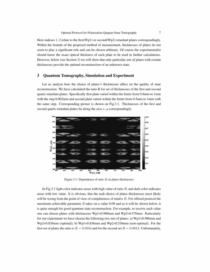
Let us analyze how the choice of plates’s thicknesses affect on the quality of statereconstruction. We have calculated the ratio R for set of thicknesses of the first and secondquartz retardant plates. Specifically first plate varied within the limits from 0.8mm to 1mmwith the step 0.002mm and second plate varied within the limits from 0.5mm to 1mm withthe same step. Corresponding picture is shown on Fig.3.1. Thicknesses of the first andsecond quarts retardant plates lie along the axis x, y correspondingly.

Figure 3.1: Dependence of ratio R on plates thicknesses

In Fig.3.1 light color indicates areas with high value of ratio R, and dark color indicatesareas with low value. It is obvious, that the rash choice of plates thicknesses most likelywill be wrong from the point of view of completeness of matrix B. For offered protocol themaximum achievable parameter R takes on a value 0.09 and as it will be shown below, itis quite enough for good quantum state reconstruction. For example, to receive such valueone can choose plates with thicknesses Wp1=0.988mm and Wp2=0.570mm. Particularlyfor our experiment we have chosen the following two sets of plates: a) Wp1=0.988mm andWp2=0.836mm (optimal); b) Wp1=0.836mm and Wp2=0.536mm (non-optimal). For thefirst set of plates the ratio is R = 0.0554 and for the second set R = 0.0013. Unfortunately,


our choice has been limited by available plates, so we were not able to check their extremalvalues.

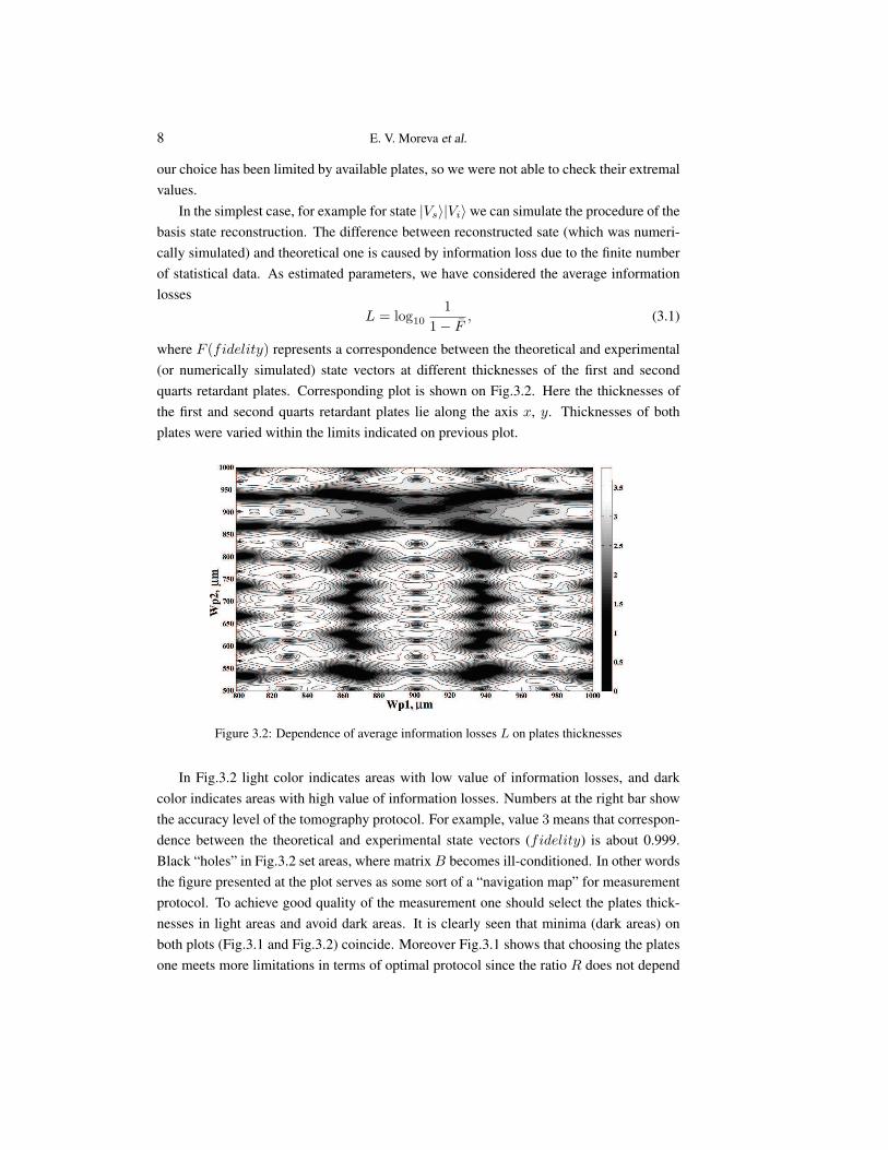
In the simplest case, for example for state |Vs〉|Vi〉 we can simulate the procedure of thebasis state reconstruction. The difference between reconstructed sate (which was numeri-cally simulated) and theoretical one is caused by information loss due to the finite numberof statistical data. As estimated parameters, we have considered the average informationlosses

L = log10

11− F

, (3.1)

where F (fidelity) represents a correspondence between the theoretical and experimental(or numerically simulated) state vectors at different thicknesses of the first and secondquarts retardant plates. Corresponding plot is shown on Fig.3.2. Here the thicknesses ofthe first and second quarts retardant plates lie along the axis x, y. Thicknesses of bothplates were varied within the limits indicated on previous plot.

Figure 3.2: Dependence of average information losses L on plates thicknesses

In Fig.3.2 light color indicates areas with low value of information losses, and darkcolor indicates areas with high value of information losses. Numbers at the right bar showthe accuracy level of the tomography protocol. For example, value 3 means that correspon-dence between the theoretical and experimental state vectors (fidelity) is about 0.999.Black “holes” in Fig.3.2 set areas, where matrix B becomes ill-conditioned. In other wordsthe figure presented at the plot serves as some sort of a “navigation map” for measurementprotocol. To achieve good quality of the measurement one should select the plates thick-nesses in light areas and avoid dark areas. It is clearly seen that minima (dark areas) onboth plots (Fig.3.1 and Fig.3.2) coincide. Moreover Fig.3.1 shows that choosing the platesone meets more limitations in terms of optimal protocol since the ratio R does not depend


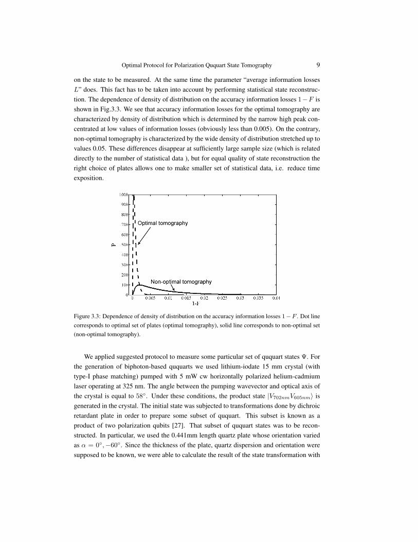
on the state to be measured. At the same time the parameter “average information lossesL” does. This fact has to be taken into account by performing statistical state reconstruc-tion. The dependence of density of distribution on the accuracy information losses 1−F isshown in Fig.3.3. We see that accuracy information losses for the optimal tomography arecharacterized by density of distribution which is determined by the narrow high peak con-centrated at low values of information losses (obviously less than 0.005). On the contrary,non-optimal tomography is characterized by the wide density of distribution stretched up tovalues 0.05. These differences disappear at sufficiently large sample size (which is relateddirectly to the number of statistical data ), but for equal quality of state reconstruction theright choice of plates allows one to make smaller set of statistical data, i.e. reduce timeexposition.

Figure 3.3: Dependence of density of distribution on the accuracy information losses 1−F . Dot linecorresponds to optimal set of plates (optimal tomography), solid line corresponds to non-optimal set(non-optimal tomography).

We applied suggested protocol to measure some particular set of ququart states Ψ. Forthe generation of biphoton-based ququarts we used lithium-iodate 15 mm crystal (withtype-I phase matching) pumped with 5 mW cw horizontally polarized helium-cadmiumlaser operating at 325 nm. The angle between the pumping wavevector and optical axis ofthe crystal is equal to 58◦. Under these conditions, the product state |V702nmV605nm〉 isgenerated in the crystal. The initial state was subjected to transformations done by dichroicretardant plate in order to prepare some subset of ququart. This subset is known as aproduct of two polarization qubits [27]. That subset of ququart states was to be recon-structed. In particular, we used the 0.441mm length quartz plate whose orientation variedas α = 0◦,−60◦. Since the thickness of the plate, quartz dispersion and orientation weresupposed to be known, we were able to calculate the result of the state transformation with


high accuracy. In measurement part of setup we used two sets of retardant plates withdifferent thicknesses, optimal and non-optimal, and made the reconstruction procedure ofququarts states at the fixed set of statistical data for each set. In both series of experi-ments we gathered identical statistic equal 30-35 thousands events. According to protocol,four sets of measurements were performed for each input state, so totally we performed144 measurements of the coincidence rate as a function of orientation angles of Wp1 andWp2. While accumulating experimental data, the accidental coincidence rate Nacc, whichis expressed in terms of the rate of averaged single counts from each photodetector andthe coincidence-window width (T ) of the scheme as Nacc = 〈N1〉〈N2〉T , is extractedfrom the total coincidence rate. For state reconstruction we used the maximum likelihoodmethod, that was developed in [4] and was successively applied to reconstruct states ofoptical qutrits [5]. The result of ququarts reconstruction is given in Table 3.1. The value

Table 3.1: The result of ququarts reconstruction

fidelityα (deg.) optimal set non-optimal set

0 0.999 0.974−60 0.993 0.975

of parameter F is defined as F = |〈ctheory|cexp〉|2. It is clearly seen that obtained fidelityvalues for optimal set of thicknesses is much higher than for non-optimal set. Fidelity forall states in the first case (optimal) was above 0.99, in the second case (non-optimal) fidelitywas about 0.97.

4 Conclusion

In conclusion, we have suggested and tested an optimal protocol for polarizationququarts state tomography. The protocol allows one to achieve highest accuracy of the statereconstruction with available resources which experimentalist holds in his hands while do-ing particular measurements. Then we investigated theoretically and experimentally theaccuracy of polarization ququart reconstruction depending on parameters available in ex-periment (quartz plates thicknesses) at fixed set of statistical data. The developed method-ology can be extended easily to other quantum states reconstruction as well as used foroptimization of various technological parameters of quantum tomography protocols.

Acknowledgments

This work was supported, in part, by Russian Foundation for Basic Research (Projects06-02-16769 and 06-02-39015) and by the Leading Russian Scientific Schools (Project796.2008.2). E. V. Moreva acknowledges the support from the Dynasty Foundation.


References

[1] Yu. I. Bogdanov, Root Estimator of Quantum States, quant-ph.0303014 (2003), 1–26.[2] Yu. I. Bogdanov, Quantum states estimation: root approach, quant-ph.0310011

(2003), 1–11.[3] Yu. I. Bogdanov, Statistical inverse problem: root approach, quant-ph.0312042

(2003), 1–17.[4] Yu. I. Bogdanov, Fundamental notions of classical and quantum statistics: a root

approach, Optics and Spectroscopy 96 (2004), 668–678.[5] Yu. I. Bogdanov, M. V. Chekhova, L. A. Krivitsky, S. P. Kulik, A. N. Penin, A. A.

Zhukov, L. C. Kwek, C. H. Oh, and M. K. Tey, Statistical reconstruction of qutrits,Phys. Rev. A 70 (2004), 042303-1–042303-16.

[6] Yu. I. Bogdanov, M. V. Chekhova, S. P. Kulik, G. A. Maslennikov, A. A. Zhukov, C.H. Oh, and M. K. Tey, Qutrit state engineering with biphotons, Phys. Rev. Lett. 93(2004), 23503-1–23503-4.

[7] Yu. I. Bogdanov, L. A. Krivitsky, and S. P. Kulik, Statistical reconstruction of opticalthree-level quantum states, J. Exp. Theor. Phys. Lett. 78 (2003), 352–357.

[8] Yu. I. Bogdanov, E. V. Moreva, A. K. Gavrichenko, I. V. Tikhonov, and S. P. Kulik, tobe published.

[9] Yu. I. Bogdanov, E. V. Moreva, G. A. Maslennikov, R. F. Galeev, S. S. Straupe, and S.P. Kulik, Polarization states of four-dimensional systems based on biphotons, Phys.Rev. A. 73 (2006), 063810-1–063810-13.

[10] G. M. DAriano, P. Mataloni and M. F. Sacchi, Generating qudits with d = 3, 4 en-coded on two-photon states, quant-ph/0503227, (2005), 1–4.

[11] M. Genovese, P. Traina, Review on qudits production and their application to quantumcommunication and studies on local realism, quant-ph.07111288, (2007), 1–23.

[12] D. F. V. James, P. G. Kwiat, W. J. Munro and A. G. White, Measurement of qubits,Phys. Rev. A 64 (2001), 052312-1–052312-15.

[13] V. P. Karassiov, Polarization structure of quantum light fields: a new insight, I. Gen-eral outlook, J. Phys. A 26 (1993), 4345–4354.

[14] V. P. Karassiov, S. P. Kulik, Polarization transformations of multimode light fields, J.Exp. Theor. Phys. 104 (2007), 30–46.

[15] D. N. Klyshko, Polarization of light: fourth-order effects and polarization-squeezedstates, J. Exp. Theor. Phys. 84 (1997), 1065–1079.

[16] L. A. Krivitsky, S. P. Kulik, A. N. Penin, and M.V. Chekhova, Biphotons as three-levelsystems: transformation and measurement, J. Exp. Theor. Phys. 97 (2003), 846–857.

[17] J. C. Howell, A. Lamas-Linares, and D. Bouwmeester, Experimental violation of aspin-1 bell inequality using maximally entangled four-photon states, Phys. Rev. Lett.88 (2002), 030401-1–030401-4.

[18] N. K. Langford, R. B. Dalton, M. D. Harvey, J. L. OBrien, G. J. Pryde, A. Gilchrist, S.D. Bartlett, and A. G. White, Measuring entangled qutrits and their use for quantumbit commitment, Phys. Rev. Lett. 93 (2004), 053601-1–053601-4.


[19] A. Mair, A. Vaziri, G. Weihs, and A. Zeilinger, Entanglement of the orbital angularmomentum states of photons, Nature 412 (2001), 313–316.

[20] L. Neves, G. Lima, J. A. Gomez, C. Monken, C. Saavedra, and S. Padua, Generationof entangled states of qudits using twin photons, Phys. Rev. Lett. 94 (2005), 100501-1–100501-4.

[21] M. N. OSullivan-Hale, I. A. Khan, R. W. Boyd, and J. C. Howell, Pixel entanglement:experimental realization of optically entangled d = 3 and d = 6 qudits, Phys. Rev.Lett. 94 (2005), 220501-1–220501-4.

[22] J. Rehacek, B.-G. Englert, and D. Kaszlikowski, Minimal qubit tomography, Phys.Rev. A 70 (2004), 052321-1–052321-13.

[23] Hd. Riedmatten, I. Marcikic, V. Scarani, W. Tittel, H. Zbinden, and N. Gisin, Tailoringphotonic entanglement in high-dimensional Hilbert spaces, Phys. Rev. A 69 (2004),050304-1–050304-4(R).

[24] R. Thew, A. Acin, H.Zbinden, and N. Gisin, Bell-type test of energy-time entangledqutrits, Phys. Rev. Lett. 93 (2004), 010503-1–010503-4.

[25] A. Vaziri, G. Weihs, and A. Zeilinger, Experimental two-photon, three-dimensionalentanglement for quantum communication, Phys. Rev. Lett. 89 (2002), 240401-1–240401-4.

[26] S. Walborn, D. Lemelle, M. Almeida, and P. Ribeiro, Quantum key distribution withhigher-order alphabets using spatially-encoded qudits, qunt- ph/0510088, (2006), 1–4.

[27] Since we started with the product state |V702nmV605nm〉 its zero entanglement degreeremains constant under local polarization transformations.

optimal protocol for polarization ququart state … · optimal protocol for polarization ququart...

Documents