Optimal Zielonka-Type Construction ofDeterministic Asynchronous Automata

Blaise Genest1,2, Hugo Gimbert3, Anca Muscholl3, Igor Walukiewicz3

1 CNRS, IPAL UMI, joint with I2R-A*STAR-NUS, Singapore2 CNRS, IRISA UMR, joint with Universite Rennes I, France

3 LaBRI, CNRS/Universite Bordeaux, France

Abstract. Asynchronous automata are parallel compositions of finite-state processes synchronizing over shared variables. A deep theorem dueto Zielonka says that every regular trace language can be represented bya deterministic asynchronous automaton. In this paper we improve theconstruction, in that the size of the obtained asynchronous automatonis polynomial in the size of a given DFA and simply exponential in thenumber of processes. We show that our construction is optimal within theclass of automata produced by Zielonka-type constructions. In particular,we provide the first non trivial lower bound on the size of asynchronousautomata.

1 Introduction

Zielonka’s asynchronous automata [15] is probably one of the simplest, and yetrich, models of distributed computation. This model has a solid theoretical foun-dation based on the theory of Mazurkiewicz traces [9,4]. The key property ofasynchronous automata, known as Zielonka’s theorem, is that every regular tracelanguage can be represented by a deterministic asynchronous automaton [15].This result is one of the central results on distributed systems and has beenapplied in many contexts. Its complex proof has been revisited on numerous oc-casions (see e.g. [2,3,12,13,6] for a selection of such papers). In particular somesignificant complexity gains have been achieved since the original construction.This paper provides yet another such improvement, and moreover it shows thatthe presented construction is in some sense optimal.

The asynchronous automata model is basically a parallel composition offinite-state processes synchronizing over shared (state) variables. Zielonka’s the-orem has many interpretations, here we would like to consider it as a resultabout distributed synthesis: it gives a method to construct a deterministic asyn-chronous automaton from a given sequential one and a distribution of the actionsover the set of processes. We remark that in this context it is essential that theconstruction gives a deterministic asynchronous automaton: for a controller it isthe behaviour and not language acceptance that is important. The result has ap-plications beyond the asynchronous automata model, for example it can be usedto synthesize communicating automata with bounded communication channels

2

[11,7] or existentially-bounded channels [5]. Despite these achievements, fromthe point of view of applications, the biggest problem of constructions of asyn-chronous automata is considered to be their high complexity. The best construc-tions give either automata of size doubly exponential in the number of processes,or exponential in the size of the sequential automaton.

This paper proposes an improved construction of deterministic asynchronousautomata. It offers the first algorithm that gives an automaton of size polyno-mial in the size of the sequential automaton and exponential in the number ofprocesses. We show that this is optimal for Zielonka-type constructions. Namelyconstructions where each component has complete information about his history.For this we introduce the notion of locally rejecting asynchronous automatonand remark that all Zielonka-type constructions produce this kind of automata.To be locally rejecting means that a process should reject as soon as its historytells him that no more accepting extension exists. We believe that a locally re-jecting behavior is quite desirable for applications, such as monitoring or control.We show that when transforming a deterministic word automaton to a deter-ministic locally rejecting automaton, the exponential blow-up in the number ofcomponents is unavoidable. Thus, to improve our construction one would needto construct automata that are not locally rejecting. However no general toolsfor doing this are available at present.

For the upper bound we start from a deterministic (I-diamond) word au-tomaton. We think that this is the best point of departure for a study of thecomplexity of constructing asynchronous automata: considering non determin-istic automata would introduce costs related to determinization. The size of thedeterministic asynchronous automaton obtained is measured as the sum of thesizes of the local states sets. It means that we do not take global accepting statesinto account. We think that this is reasonable as it is hardly practical to list thesestates explicitly. From a deterministic I-diamond automaton A and a distributedalphabet with process set P, we construct a deterministic asynchronous automa-ton of size 22·|P|4 · |A||P|2 . We believe that this complexity, although exponentialin the number of processes, is interesting in practice. If we want to implementsuch a device then it will need memory of size logarithmic in |A| and polynomialin |P|. We also show that computing the next state on-the-fly can be done intime polynomial in both |A| and |P|.

Related work. Besides the general constructions of Zielonka type, there area couple of different constructions, however they either apply to subclasses ofregular trace languages, or they produce non deterministic automata (or both).The first category includes [10,3], that provide deterministic asynchronous cel-lular automata from a given trace homomorphism in case that the dependencealphabet is acyclic and chordal, respectively. These constructions are quite sim-ple and only polynomial in the size of the monoid (thus still exponential in thesize of a DFA). In the second category we find [16], who gives an inductive con-struction for non deterministic, deadlock-free asynchronous cellular automata.(A deadlock-free variant of Zielonka’s construction was proposed in [14]). Thepaper [1] proposes a construction of asynchronous automata of size exponential

3

only in the number of processes (and polynomial in |A|) as our construction, butit yields non deterministic asynchronous automata (inappropriate for monitoringor control). Notice that while asynchronous automata can be determinized, thereare cases where the blow-up is doubly exponential in the number of processes [8].

2 Preliminaries

We fix a finite set P of processes and a finite alphabet Σ. Each letter a ∈ Σ is anaction associated with the set of processes dom(a) ⊆ P involved in its execution.A pair (Σ,dom) is called distributed alphabet. A deterministic automaton overthe alphabet Σ is a tuple A = 〈Q,Σ,∆, q0, F 〉 with a finite set of states Q, a setof final states F , an initial state q0 and a transition function ∆ : Q × Σ → Q.As usual we extend ∆ to words in Σ∗. We use L(A) to denote the languageaccepted by A. The automaton accepts w ∈ Σ∗ if ∆(q0, w) ∈ F . The size |A| ofA is the number of its states.

Concurrent systems with shared actions given by a distributed alphabet(Σ,dom), are readily modeled by Mazurkiewicz traces [9]. The idea is thatthe distribution of the alphabet defines an independence relation among actionsI ⊆ Σ×Σ, by setting (a, b) ∈ I if and only if dom(a)∩dom(b) = ∅. We call (Σ, I)an independence alphabet. The independence relation induces a congruence ∼ onΣ∗ by setting u ∼ v if there exist words u1, . . . , un ∈ Σ∗ with u1 = u, un = vand such that for every i < n we have ui = xaby, ui+1 = xbay for some x, y ∈ Σ∗and (a, b) ∈ I. An ∼-equivalence class is simply called a (Mazurkiewicz) trace.We denote by [u] the trace associated with the word u ∈ Σ∗ (for simplicity wedo not refer to I, neither in ∼ nor in [u], as the independence alphabet is fixed).Trace prefixes and trace factors are defined as usual, with [p] a trace prefix (tracefactor, resp.) of [u] if p is a word prefix (word factor, resp.) of some v ∼ u. Fortwo prefixes T1, T2 of T , we let T1 ∪ T2 denote the smallest prefix T ′ of T suchthat Ti ≤ T ′ for i = 1, 2.

For several purposes it is convenient to represent traces by (labeled) pomsets.Formally, a trace T = [a1 · · · an] (ai ∈ Σ for all i) corresponds to a labeled pomset(E, λ,≤) defined as follows: E = e1, . . . , en is a set of events (or nodes), onefor each position in T . Event ei is labeled by λ(ei) = ai, for each i. The relation≤ is the least partial order on E with ei ≤ ej whenever (ai, aj) ∈ D and i ≤ j. InFigure 1 we give an example for the pomset of a trace T , depicted by its Hassediagram. A total order e1 · · · en that is compatible with ≤ is called a linearizationof T .

An automaton A is called I-diamond if for all (a, b) ∈ I, and s a state of A:∆(s, ab) = ∆(s, ba). Note that the I-diamond property implies that the languageof A is I-closed : that is, u ∈ L(A) if and only if v ∈ L(A) for every u ∼ v. Thispermits us to write ∆(s, T ) where T is a trace, to denote the state reached by Afrom s on some linearization of T . Languages of I-diamond automata is calledregular trace languages.

Definition 1. A deterministic asynchronous automaton over the distributed al-phabet (Σ, dom) is a tuple B = 〈(Sp)p∈P , (δa)a∈Σ , s0,Acc〉 where:

4

c

b

c

a

d

b b

d

a

p

q

r

Fig. 1. The pomset associated with the trace T = [c b a d c b a d b], with dom(a) =p, q, dom(b) = q, r, dom(c) = p, dom(d) = r.

– Sp is the finite set of local states of a process p ∈ P,– δa :

∏q∈dom(a) Sq →

∏q∈dom(a) Sq is the local transition function associated

with an action a ∈ Σ,– s0 ∈

∏p∈P Sp is the global initial state,

– Acc ⊆∏p∈P Sp is a set of global accepting states.

We call∏p∈P Sp the set of global states (whereas Sp is the set of p-local

states). In this paper the size of an asynchronous automaton B is the totalnumber of local states

∑p∈P |Sp|. This definition is very conservative, as one

may want to count also Acc or the transition functions (which can be exponentialin |B|). We will see that our construction allows to compute both Acc and thetransition functions in polynomial time.

With the asynchronous automaton B one can associate a global automatonAB = 〈Q,Σ,∆, q0,Acc〉 where:

– The set of states is the set of global states Q =∏p∈P Sp of B, the initial

and the accepting states are as in B.– The transition function ∆ : Q×Σ → Q is defined by ∆(s, a) = (s′p)p∈P with

(s′p)p∈dom(a) = δa((sp)p∈dom(a)) and s′p = sp, for every p /∈ dom(a).

Clearly AB is a finite deterministic automaton with the I-diamond property.

Definition 2. The language of an asynchronous automaton B is the languageof the associated global automaton AB.

We conclude this section by introducing some notions that are basic ingredi-ents of the common constructions of asynchronous automata. For a trace T , wedenote by dom(T ) =

⋃e∈T dom(λ(e)) the set of processes occurring in T . For a

process p ∈ P, we denote by prefp(T ) the minimal trace prefix of T containingall events of T on process p. Hence, prefp(T ) has a unique maximal event thatis the last (most recent) event of T on process p. This maximal event is denotedas lastp(T ). Intuitively, prefp(T ) corresponds to the history of process p afterexecuting T . We extend this notation to a set of processes P ⊆ P and denote byprefP (T ) the minimal trace prefix containing all events of T on processes fromP . For example, in Figure 1 we have prefp(T ) = [cbadcba] and lastp(T ) is thesecond a of the pomset.

5

3 Zielonka-type constructions: state of the art

All general constructions of deterministic asynchronous automata basically fol-low the main ideas of the original construction of Zielonka [15]. These con-structions start with a regular, I-closed word language, that is given either by ahomomorphism to a finite monoid, or by an I-diamond automaton. In most appli-cations we are interested in the second case, where we start with a (possibly nondeterministic) automaton. The general constructions yield either asynchronousautomata as defined in the previous section, or asynchronous cellular automata,that correspond to a concurrent-read-owner-write model.

Theorem 1. [15] Let A be an I-diamond automaton over the independencealphabet (Σ, I). A deterministic asynchronous automaton B can be effectivelyconstructed with L(A) = L(B).

We now review the constructions of [2,12,6] and recall their complexities. Itis well known that determinization of word automata requires an exponentialblow-up, hence the complexity of going from a non deterministic I-diamond au-tomaton A to a deterministic asynchronous automaton is at least exponentialin |A|. In that case, [6] gives an optimal construction in that it is simply expo-nential. Since determinization has little to do with concurrency, we assume fromnow on that A is a deterministic automaton.

– [2] introduces asynchronous mappings and constructs asynchronous cellularautomata of size |Σ||Σ|2 · |A|2|Σ| .

– [12] constructs asynchronous automata of size |P||P2| · |A||A|·2|P| .– [6] introduces zone decompositions and constructs asynchronous automata

of size 23|P3| · |A||A|·|P|2 .

Comparing our present construction with previous ones, we obtain asyn-chronous automata of size 22|P|4 · |A||P|2 . In all these constructions, the obtainedautomata are such that every process knows the state reached by A on its his-tory. We abstract this property below, and show in the following section thatour construction is optimal in this case.

Definition 3. A deterministic asynchronous automaton B is called locally re-jecting if for every process p, there is a set Rp ⊆ Sp such that for every traceT :

prefp(T ) /∈ pref(L(B)) iff the p-local state reached by B on T is in Rp.

Notice that Rp is a trap: if B reaches Rp on trace T , then so it does on everyextension of T ≤ T ′. Obviously, no accepting global state of B has a componentin Rp. For these reasons we call states of Rp rejecting.

Let us justify the interest in locally rejecting automata by an observation thatall general constructions [15,2,3,13,12,6] of deterministic asynchronous automataproduce such automata. Let us assume thatA is a (possibly non deterministic) I-diamond automaton, and B a deterministic asynchronous automaton produced

6

by one of the constructions in [15,13,12,6] (a similar statement applies to theasynchronous cellular automata in [2,3]). Then the local p-state sp reached byB after processing the trace T determines the set of states reached by A onprefp(T ), for every process p. Thus, if no state in this set can reach a final stateof A, then we put sp in Rp. This makes B locally rejecting.

4 An exponential lower bound

In this section we present our lower bound result. We show that transformingan I-diamond deterministic automaton into a locally rejecting asynchronous au-tomaton may induce an exponential blow-up in the number of processes. For thiswe define a family of languages Pathn, such that the minimal sequential automa-ton for Pathn has size O(n2) but every locally rejecting automaton recognizingPathn is of size at least 2n/4.

Let P = 1, . . . , n be the set of processes. The letters of our alphabet arepairs of processes, two letters are dependent if they have a process in common.Formally, the distributed alphabet is Σ =

(P2

)with dom(p, q) = p, q.

The language Pathn is the set of traces [x1 · · ·xk] such that every two con-secutive letters have a process in common: xi ∩ xi+1 6= ∅ for i = 1, . . . , k − 1.Observe that a deterministic sequential automaton recognizing this languagesimply needs to remember the last letter it has read. So it has less than |P|2states.

Theorem 2. Every locally rejecting asynchronous automaton recognizing Pathnis of size at least 2n/4.

Proof. Take a locally rejecting automaton recognizing Pathn. Without loss ofgenerality we suppose that n = 4k. To get a contradiction we suppose thatprocess n of this automaton has less than 2k (local) states.

We define for every integer 0 ≤ m < k two traces: am = 4m, 4m+ 14m+1, 4m+24m+2, 4m+4 and bm = 4m, 4m+14m, 4m+34m+3, 4m+4.To get some intuition, the reader may depict traces a0 and b0 and see that botha0 and b0 form a path from process 0 to process 4, the difference is that tracea0 goes through process 2 while trace b0 goes through process 3.

Consider the language L defined by the regular expression (a0 + b0)(a1 +b1) · · · (ak−1 + bk−1). Clearly, language L is included in Pathn and contains 2k =2n/4 different traces. As we have assumed that process n has less than 2k states,there are two different traces t1, t2 from L such that process n is in the samestate after t1 and t2. For simplicity of presentation we assume that t1 and t2differ on the first factor: t1 starts with a0, and t2 with b0.

We can remark that processes 0 and n are in the same state after readingt10, 3 and t2. For process 0 it is clear as in both traces it sees the same trace0, 10, 3. By our hypothesis, process n is in the same local state after tracest1 and t2, therefore also after traces t10, 3 and t2.

Consider now the state sn reached by n after reading t20, n. Since t20, n ∈Pathn, we have sn /∈ Rn. By the above, the same state sn is also reached after

7

reading t10, 30, n. Trace t1 starts with a0 = 0, 11, 22, 4 and continueswith processes whose numbers are greater than 4, so 0, 3 commutes with allletters of t1 except 0, 1. Hence t10, 3 6∈ pref(Pathn). Since trace t1 endswith an action of process n, we have prefn(t10, 30, n) = t10, 30, n /∈pref(Pathn). Since we have assumed that the automaton is locally rejecting,sn ∈ Rn. A contradiction. 2

5 A matching upper bound

Our goal is to modify the construction from [6] in order to make it polynomialwith respect to the size of the sequential automaton. We give an overview ofthe new construction, first describing the objects the asynchronous automatonmanipulates. Some details of the mechanics of the automaton will follow (a moredetailed presentation can be found in the appendix).

We fix a set of processes P and a distributed alphabet (Σ,dom). Let A =〈Q,Σ,∆, q0, F 〉 be a deterministic I-diamond automaton. A candidate for anequivalent asynchronous automaton B = 〈(Sp)p∈P , (δa)a∈Σ , s0,Acc〉 has a set ofstates for each process and a local transition function. The goal is to make Bcalculate the state reached by A after reading a linearization of a trace T . Let usexamine how B can accomplish this task. After reading a trace T the local stateof a component p of B depends only on prefp(T ). Hence, B can try to calculatethe state reached by A after reading (some linearization of ) prefp(T ). When anext action, say a, is executed, processes in dom(a) can see each others’ statesand make the changes accordingly. Intuitively, this means that these processescan now compose their information in order to calculate the state reached byA on T ′ = prefdom(a)(T ) a. To do so they will need some information about thestructure of the trace.

As usual, the tricky part of this process is to reconstruct the common viewof prefdom(a)(T ) from separate views of each process: prefp(T ) for p ∈ dom(a).For the sake of example suppose that dom(a) = p, q, r, and we know the statesreached by A after reading prefp(T ), prefq(T ), and prefr(T ). We would like toknow the state of A after reading prefp,q,r(T ). This would be possible if wecould compute contributions of prefq(T ) \ prefp(T ) and prefr(T ) \ prefp,q(T ).The automaton B should be able to do this by looking at sp, sq, and sr, only.This remark points out the challenge of the construction: find the type infor-mation that allows to deduce the behaviour of A, and that at the same time isupdatable by an asynchronous automaton, see e.g. [13]. As in all general Zielonkaconstructions, we use the fact that e.g. prefr(T )∩prefp,q(T ) is uniquely deter-mined by last(prefr(T )) ∩ last(prefp,q(T )) ([15], see also [13]). By last(U) wedenote the set of events lastp(U) | p ∈ P.

5.1 General structure

Before introducing formal definitions it may be worth to say what is the generalstructure of the states of the automaton B. Every local state will be a triple(ts, ZO,∆), where

8

– ts will be a time stamping information as in all general constructions ofasynchronous automata;

– ZO will be a zone order, a bounded size partial order on a partition of thetrace;

– ∆ will be state information, recording the behavior of A on the partitiongiven by ZO.

Roughly, we will use time stamping to compute zone orders, and zone ordersto compute state information. The latter provides all the necessary informationabout the behaviour of A on (a linearization of) the trace.

Timestamping: The goal of the time stamping function [15] is to determinefor a set of processes P and a process q the set last(prefP (T )) ∩ last(prefq(T )).This set uniquely determines the intersection of prefP (T ) and prefq(T ) (fordetails see e.g. [13]). Computing such intersections is essential when compos-ing information about prefp(T ) for every p ∈ dom(a) to information aboutprefdom(a)(T ). The main point is that there exists a deterministic asynchronousautomaton that can accomplish this task (for a formal description see the ap-pendix). Each of its local states can be described with O(|P|2 log(|P|) bits.

For instance, if a new b is executed after T = [cbadcbad] in Figure 2, processesq, r determine that the intersection of their last-sets consists of the second b.Indeed, last(prefq(T )) is made of the second a (for lastp = lastq) and the secondb (for lastr). Also, last(prefr(T )) is made of the second d (for lastr), the secondb (for lastq) and the first a (for lastp).

Zone orders: Recall that one of our objectives is to calculate, for everyp ∈ P, the state reached by A on prefp(P). As the discussion on page 7 pointedout, for this we may need to recover the transition function of A associated withprefq(T ) \ prefP (T ) for a process q and a set of processes P . Hence we needto store information about the behaviour of A on some relevant factors of Tthat are not prefixes. Zones are such relevant factors. They are defined in such away that there is a bound on the number of zones in a trace. The other crucialproperty of zones is that for every extension T ′ of T and P ⊆ P, q ∈ P, if a zoneof T intersects prefq(T ′) \ prefP (T ′) then it is entirely in this set. A zone orderwill be an abstract representation of the decomposition of a trace into zones.

Definition 4. [6] Let T = 〈E,≤, λ〉 be a trace. For an event e ∈ E we definethe set of events L(e) = f ∈ last(T ) | e ≤ f. We say that two events e, e′ areequivalent (denoted as e ≡ e′) if L(e) = L(e′). The equivalence classes of ≡ arecalled zones. The set of processes that are active in Z is denoted by dom(Z).

There is a useful partial order on zones that we define now. Let Z,Z ′ be twozones of some trace T . We write Z l Z ′ if Z 6= Z ′ and e < e′ for some eventse ∈ Z, e′ ∈ Z ′. It is easy to see that ZlZ ′ implies that L(Z ′) ( L(Z). Thanks tothis property we can define the order on zones, denoted Z ≤ Z ′, as the smallestpartial order containing the l relation.

Lemma 1. A trace is partitioned in at most |P|2 zones.

9

c

b

c

a

d

b

d

a

p

q

r

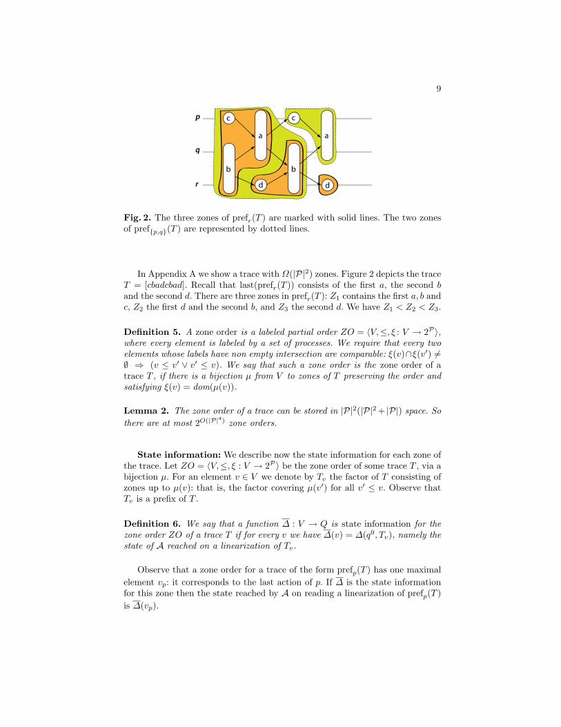
Fig. 2. The three zones of prefr(T ) are marked with solid lines. The two zonesof prefp,q(T ) are represented by dotted lines.

In Appendix A we show a trace with Ω(|P|2) zones. Figure 2 depicts the traceT = [cbadcbad]. Recall that last(prefr(T )) consists of the first a, the second band the second d. There are three zones in prefr(T ): Z1 contains the first a, b andc, Z2 the first d and the second b, and Z3 the second d. We have Z1 < Z2 < Z3.

Definition 5. A zone order is a labeled partial order ZO = 〈V,≤, ξ : V → 2P〉,where every element is labeled by a set of processes. We require that every twoelements whose labels have non empty intersection are comparable: ξ(v)∩ξ(v′) 6=∅ ⇒ (v ≤ v′ ∨ v′ ≤ v). We say that such a zone order is the zone order of atrace T , if there is a bijection µ from V to zones of T preserving the order andsatisfying ξ(v) = dom(µ(v)).

Lemma 2. The zone order of a trace can be stored in |P|2(|P|2 + |P|) space. Sothere are at most 2O(|P|4) zone orders.

State information: We describe now the state information for each zone ofthe trace. Let ZO = 〈V,≤, ξ : V → 2P〉 be the zone order of some trace T , via abijection µ. For an element v ∈ V we denote by Tv the factor of T consisting ofzones up to µ(v): that is, the factor covering µ(v′) for all v′ ≤ v. Observe thatTv is a prefix of T .

Definition 6. We say that a function ∆ : V → Q is state information for thezone order ZO of a trace T if for every v we have ∆(v) = ∆(q0, Tv), namely thestate of A reached on a linearization of Tv.

Observe that a zone order for a trace of the form prefp(T ) has one maximalelement vp: it corresponds to the last action of p. If ∆ is the state informationfor this zone then the state reached by A on reading a linearization of prefp(T )is ∆(vp).

10

5.2 The construction of the asynchronous automaton

Let us come back to the description of the asynchronous automaton B. For everyp ∈ P, a local state of Sp will have the form (tsp, ZOp,∆p). The automaton willbe defined in such a way that after reading a trace T the state sp reached at thecomponent p will satisfy:

– tsp is the time stamping information [13];– ZOp is the zone order of prefp(T );– ∆p is the state information for ZOp.

By [13] we know that B can update the tsp component. The proposition be-low says that B can update the ZOp and ∆p components (for the proof seeAppendix C).

Proposition 1. Let T be a trace and a ∈ Σ an action. Suppose that for everyp ∈ dom(a) we have the time stamping information tsp and the zone order withstate information (ZOp,∆p) of prefp(T ). We can then calculate the zone orderand the state information of prefp(Ta), for every p ∈ dom(a).

We also need to define the set of local rejecting states Rp and the globalaccepting states Acc of B. Observe that by Proposition 1, from the local state spwe can calculate ∆(q0,prefp(T )), namely the state of A reached after reading alinearization of prefp(T ). This state is exactly the state associated to the uniquemaximal element of the zone order in sp. Hence, B can be made locally rejectingby letting sp ∈ Rp if ∆(q0,prefp(T )) is a deadend state of A.

To define accepting tuples of states of B we use the following proposition:

Proposition 2. Let T be a trace. Given for every p ∈ P the time stamping tsp,and the zone order ZOp with state information ∆p of prefp(T ), we can calculate∆(q0, T ), the state reached by A on a linearization of T .

In the light of Proposition 2, a tuple of states of B is accepting if the state∆(q0, T ) of A is accepting. The two propositions give us:

Theorem 3. Let A be a deterministic I-diamond automaton over the distributedalphabet (Σ, dom). We can construct an equivalent deterministic locally rejectingasynchronous automaton B with at most 22|P|4 · |A||P|2 states.

We now describe informally the main ingredients of the proof of Proposition 1(Proposition 2 goes along similar lines). The zone order ZO of prefP∪q(T ) isbuilt in two steps from ZOP and ZOq: first we construct a so-called pre-zoneorder ZO′ by adding to ZOP the zones from prefq(T ) \ prefP (T ) [6]. Thenwe quotient ZO′ in order to obtain ZO. The quotient operation amounts tomerge zones. The difficulty compared to [6] is posed by the update of the stateinformation. Since the state information for the pre-zone ZO′ is inconsistent dueto the merge, the crucial step is to compute this information on downward closedsets of zones:

11

Lemma 3. Let ZO = 〈V,≤, ξ〉, ∆ be the zone order and state information for atrace T (via the bijection µ). For every downward closed B ⊆ V we can computethe state reached by A on a linearization of TB =

⋃Tv | v ∈ B, using only ZO

and ∆.

The proof for the lemma above is based on a nice observation about I-diamond automata A, [2]. It says that for every three traces T0, T1, T2 withdom(T1) ∩ dom(T2) = ∅, the state reached by A on a linearization of T0T1T2

can be computed from dom(T1) and the states reached on (linearizations of) T0,T0T1, T0T2, respectively.

We now sketch the proof of the lemma. We first choose some linearizationv1, . . . , vn of B, and let Bi = v1, . . . , vi. Let us write Bi,k (i ≤ k) for the setBi∪vj | vj ≤ vk, j > i. We show now how to compute inductively ∆(q0, TBi,k).

Suppose we know already ∆(q0, TBi−1,k), for all k ≥ i− 1. In particular, notethat the states qi−1, qi reached on µ(v1 · · · vi−1) and µ(v1 · · · vi), respectively, areknown (cases k = i− 1 and k = i).

We compute now ∆(q0, TBi,k), for k > i. Two cases arise. If vi 6< vk thenwe apply the observation of [2] to qi−1, qi, ∆(q0, TBi−1,k), ξ(vi), which yields∆(q0, TBi,k). If vi < vk, then Bi−1,k = Bi,k and the state ∆(q0, TBi,k) is al-ready known. At the end of this polynomial time procedure, we have computed∆(q0, TB) = ∆(q0, TBn,n).

Remark 1. The automaton B of Theorem 3 can be constructed on-the-fly, i.e. giventhe action a ∈ Σ and the local states sp of B, p ∈ dom(a), one can compute thesuccessor states δa((sp)p∈dom(a). The question is now how much time we needfor this computation. The update of the time stamping and that of zone orderstakes time polynomial in |P|. The update of state information can be done intime polynomial in |P| and linear in the number of transitions of |A|. So over-all, we can compute transitions on-the-fly in polynomial time. Similarly, we candecide whether a global state is accepting in polynomial time.

6 Conclusion

In this paper we presented an improved construction of asynchronous automata.Starting from a zone construction of [6], we have shown how to keep just one stateper zone instead of a transition table. This allows to obtain the first constructionthat is polynomial in the size of the sequential automaton and exponential onlyin the number of processes.

It is tempting to conjecture that our construction is optimal. Unfortunately,it is very difficult to provide lower bounds on sizes of asynchronous automata. Wegave a matching lower bound for the subclass of locally rejecting automata. It isworth to recall that all general constructions in the literature produce automataof this kind. Moreover the concept of locally rejecting automaton is interestingon its own from the point of view of applications.

We conjecture that the translation from deterministic word automata toasynchronous automata must be exponential in the number of processes; wherethe size means the total number of local states.

12

References

1. N. Baudru. Distributed asynchronous automata. In CONCUR’09, number 5710in LNCS, pages 115–130. Springer, 2009.

2. R. Cori, Y. Metivier, and W. Zielonka. Asynchronous mappings and asynchronouscellular automata. Information and Computation, 106:159–202, 1993.

3. V. Diekert and A. Muscholl. Construction of asynchronous automata. In V. Diek-ert and G. Rozenberg, editors, Book of Traces, pages 249–267. World Scientific,Singapore, 1995.

4. V. Diekert and G. Rozenberg, editors. The Book of Traces. World Scientific,Singapore, 1995.

5. B. Genest, D. Kuske, and A. Muscholl. A Kleene theorem and model check-ing algorithms for existentially bounded communicating automata. Inf. Comput.,204(6):920–956, 2006.

6. B. Genest and A. Muscholl. Constructing exponential-size deterministic zielonkaautomata. In ICALP’06, number 4052 in LNCS, pages 565–576. Springer, 2006.

7. J. G. Henriksen, M. Mukund, K. N. Kumar, M. Sohoni, and P. S. Thiagarajan. Atheory of regular MSC languages. Inf. Comput., 202(1):1–38, 2005.

8. N. Klarlund, M. Mukund, and M. Sohoni. Determinizing asynchronous automata.In ICALP’94, number 820 in LNCS, pages 130–141. Springer, 1994.

9. A. Mazurkiewicz. Concurrent program schemes and their interpretations. DAIMIRep. PB 78, Aarhus University, Aarhus, 1977.

10. Y. Metivier. An algorithm for computing asynchronous automata in the case ofacyclic non-commutation graph. In ICALP’87, number 267 in LNCS, pages 226–236. Springer, 1987.

11. M. Mukund, K. N. Kumar, and M. Sohoni. Synthesizing distributed finite-statesystems from MSCs. In CONCUR’00, number 1877 in LNCS, pages 521–535.Springer, 2000.

12. M. Mukund and M. Sohoni. Gossiping, asynchronous automata and Zielonka’stheorem. Report TCS-94-2, School of Mathematics, SPIC Science Foundation,Madras, India, 1994.

13. M. Mukund and M. A. Sohoni. Keeping track of the latest gossip in a distributedsystem. Distributed Computing, 10(3):137–148, 1997.

14. A. Stefanescu. Automatic synthesis of distributed transition systems. PhD thesis,Universitat Stuttgart, 2006.

15. W. Zielonka. Notes on finite asynchronous automata. RAIRO–Theoretical Infor-matics and Applications, 21:99–135, 1987.

16. W. Zielonka. Safe executions of recognizable trace languages by asynchronous au-tomata. In Symposium on Logical Foundations of Computer Science, Logic at Botik’89, Pereslavl-Zalessky (USSR), number 363 in LNCS, pages 278–289. Springer,1989.

13

A A trace with many zones

Here is an example showing that there can be O(|P|2) zones in a trace. As set ofprocesses we take P = 0x, 1x, . . . , nx∪0y, 1y, . . . , ny; that is two copies of theinitial segment of natural numbers. The alphabet Σ is (ix, jy) | i, j = 0, . . . , n.So a letter is a pair of processes, and naturally, the domain of such a letter arethose two processes.

We consider a trace T where there is one event for every letter from Σ. Forsimplicity of notation we will identify the events with letters. The order betweenevents is determined by the rule

– (ix, jy) ≤ (kx, ly) if i ≥ k and j ≥ l; notice the inversion of orders.

The trace is depicted in Figure 3 where the subscripts x and y are omitted forreadability. It is easy to verify that every event (ix, jy) is a zone by itself withL(ix, jy) = 0x, . . . , ix ∪ 0y, . . . , jy.

(1,0)

(0,1)

(2,0)

(0,2)

(0,n)

(n,0)

(i+1,j+1)

(i+1,j)

(i,j+1)

(i,j)

(0,0)

Fig. 3. A trace with a big zone graph

B Time stamping

Theorem 4. [13] There exist a deterministic asynchronous automaton ATS =〈(Sp)p∈P , (∆a)a∈Σ , s0〉 such that for every trace T and state s = ∆(s0, T ) reachedby ATS after reading T :

for every P ⊆ P and q, r, r′ ∈ P, the set of local states sp | p ∈ P ∪qallows to determine if lastr(prefP (T )) = lastr′(prefq(T )).

Moreover, such ATS can be effectively computed and its local states can be de-scribed using O(|P|2 log(|P|)) bits.

14

C Updating state and zone information

In this section we show how an asynchronous automaton updates the zone or-der and the state information (Proposition 1). We will get also the proof ofProposition 2 as a side result.

Suppose that we extend a trace T by an action a ∈ Σ. We first need toconstruct the zone order and the state information of prefdom(a)(T )a, given thezone orders and state information of each of prefp(T ), p ∈ dom(a). The followingproposition implies that this is possible.

Proposition 3. Let P ⊆ P, q ∈ P and let T be a trace. Assume that we aregiven the zone orders with state information (ZOP , ∆P ), (ZOq,∆q) for prefP (T )and prefq(T ), respectively. Suppose that we also know the local states (sp)p∈P , sqreached by the time stamping automaton ATS on prefP (T ) and prefq(T ), respec-tively. Then we can compute the zone order and the state information (ZO,∆)for prefP∪q(T ).

The proof of Proposition 3 will occupy most of this section. We start withthe following crucial property of zones, that shows that the zone update can beperformed without splitting zones:

Proposition 4 ([6], Props. 1, 3). Let T be a trace, P ⊆ P and q ∈ P. Forevery zone Z of prefP (T ), we have either Z ⊆ prefP (T ) ∩ prefq(T ) or Z ⊆prefP (T ) \ prefq(T ). Moreover, if Z is a zone of prefP (T ) or prefq(T ) then Z isa factor of some zone of prefP∪q(T ).

We need also to determine which zones of prefq(T ) are within prefP (T ) ∩prefq(T ). This task uses the time stamping automaton ATS (cf. Theorem 4):

Lemma 4. Let Z be a zone of prefq(T ). Then Z ⊆ prefP (T ) ∩ prefq(T ) if andonly if Z ≤ Z ′ for some zone Z ′ of prefq(T ) such that dom(Z ′) contains processesr, r′ ∈ P with lastr(prefP (T )) = lastr′(prefq(T )).

Proof. We use the following basic fact (see e.g. [13]):

max(prefP (T ) ∩ prefq(T )) ⊆ last(prefP (T )) ∩ last(prefq(T ))

Thus, Z ⊆ prefP (T ) ∩ prefq(T ) if and only if Z ≤ Z ′ for some zone Z ′ thatcontains an event e in max(prefP (T )∩prefq(T )). For such an event e, there existr, r′ with e = lastr(prefP (T )) = lastr′(prefq(T )). 2

We now come back to the proof of Proposition 3. Given the zone ordersZOP = 〈VP ,≤P , ξP 〉 and ZOq = 〈Vq,≤q, ξq〉, we build the required ZO = 〈V,≤, ξ〉 in two steps: (i) we construct an intermediate zone order ZO′ by adding apart of ZOq to ZOP , then (ii) we need to quotient ZO′ in order to obtain ZO.

The first step is to add to ZOP the zones of ZOq included in prefq(T ) \prefP (T ). Let W ′ ⊆ Vq denote the set of zones of ZOq satisfying Lemma 4, andlet W = Vq \W ′. The zone order ZO′ = 〈V ′,≤′, χ′〉 is defined by:

15

– V ′ = VP ∪W ,– ≤′ is the least partial order containing the orders of ZOP and ZOq, and such

that ξP (v) ∩ ξq(w) 6= ∅ implies v ≤′ w, for all v ∈ VP , w ∈W ,– ξ′(v) = ξP (v) for v ∈ VP , and ξ′(v) = ξq(v) for v ∈W .

By assumption we have a bijection µP between ZOP and the zones of prefP (T );and a bijection µq between ZOq and the zones of prefq(T ). We can define a bi-jection µ′ from ZO′ to factors of T , by simply using µP for v′ ∈ VP and µq forv′ ∈W .

It should be of no surprise that ZO′ is in general not the zone order ofprefP∪q(T ). This order has some weaker property though, that we summarizein the following definition.

Definition 7. A zone order ZO = 〈V,≤, ξ : V → 2P〉 is an pre-zone order of atrace T if there is a bijection µ from V to factors of T such that

– µ preserves order and domains: ξ(v) = dom(µ(v));– (µ(v))v∈V is a partition of T into factors, and every one of them is a factor

of a zone of T .

Lemma 5. ZO′ is an pre-zone order of prefP∪q(T ), via the mapping µ′.

Proof. By definition it is clear that µ′ respects the domains and that its valuesare factors in T , as they are zones in prefP (T ) or prefq(T ). By Proposition 4 weknow that such zones are factors of zones in prefP∪q(T ). It remains to showthat µ′ preserves order. For this suppose that v′1 ≤′ v′2 in ZO′. If the two elementscome from VP then it is clear, as µ′(v′1) = µP (v′1) ≤P µP (v′2) = µ′(v′2). Similarlyif the two elements come from W . The last possible case is when v′1 ∈ Vp andv′2 ∈W . We suppose that ξP (v′1)∩ ξq(v′2) 6= ∅; the general case being an obviousextension. By preservation of domains we get dom(µ′(v′1))∩dom(µ′(v′2)) 6= ∅. Letr be a process belonging to this intersection and let e1 ∈ µ′(v′1) and e2 ∈ µ′(v′2)be events involving r. These two events are ordered. Since by definition of W ,e2 does not belong to prefP (T ), we have e1 ≤ e2. Hence µ′(v′1) ≤′ µ′(v′2). 2

Observe that this lemma implies that every zone of prefP∪q(T ) is a unionof factors of ZO′. In a second step we show how to glue together these factorsto obtain the zone order of prefP∪q(T ). We define the following equivalencerelation ≡ on V ′ × V ′: let v1 ≡ v2 if

⋃ξ′(w) | v1 ≤′ w =

⋃ξ′(w) | v2 ≤′ w.

Then let ZO = ZO′/≡ be the quotient partial order 〈V,≤, ξ〉 with

– V = V ′/≡,– ξ([v]≡) =

⋃v′≡v ξ

′(v′),– ≤ is the smallest reflexive and transitive relation satisfying: [v]≡ ≤ [w]≡ ifv′ ≤′ w′ for some v ≡ v′, w ≡ w′.

Lemma 6. If ZO′ is a pre-zone order of a trace T then the quotient ZO =ZO′/≡ is the zone order of T .

16

Proof. Let ZO′ = 〈V ′,≤′, ξ′〉 be as in the assumption of the lemma; inparticular let µ′ be the map from V ′ to factors of T showing that ZO′ is anpre-zone order. It is not difficult to check for v ∈ V ′ that⋃

ξ′(w) | v ≤′ w =⋃dom(µ′(w)) | v ≤′ w = dom(L(µ′(v)))

where L refers to the function of Definition 4 w.r.t the trace T . Notice thatL µ′ is well-defined, since each µ′(v) is included in a zone of T . Thus, v1 ≡ v2iff dom(L(µ′(v1))) = dom(L(µ′(v2))) iff L(µ′(v1)) = L(µ′(v2)) iff µ′(v1), µ′(v2)are included in the same zone of T . 2

We show in the remaining how to obtain the state information for ZO. Firstwe introduce some notation. For ZOP = 〈VP ,≤P , ξP 〉 and v ∈ VP we writeTPv for the prefix of T consisting of all factors µP (w), with w ≤P v. Moregenerally, for a downward closed subset B of ZOP we denote by TPB the prefixof T consisting of all zones µP (v) for v ∈ B. Similarly, we define T qv using ZOqand µq. Finally, Tv is defined using ZO and µ. The notations T qB and TB arealso evident.

Calculating the state information for ZO means to calculate for every v ∈ Vthe state ∆(q0, Tv) reached by A on a linearization of Tv. The following lemmasays that this amounts to compute the state information for downward closedsubsets of VP and Vq, respectively. Recall first that V ′ = VP ∪W where W ⊆ Vqis the set of zones of prefq(T ) included in prefq(T ) \ prefP (T ). We denote by[W ]≡ the set [w]≡ | w ∈W.

Lemma 7. For every v ∈ V \ [W ]≡, there is a downward closed set B of ZOPsuch that Tv = TPB . For every v ∈ [W ]≡ there is a downward closed set B ofZOq such that Tv = T qB.

Proof. By definition, Tv is a union of zones of prefP∪q(T ). By Proposition 4,Tv is either included in prefP (T ) or prefq(T ). Suppose it is included in prefP (T ),the other case being similar. The same Proposition 4 says that Tv is union ofzones of prefp(T ). Let B = w | µP (w) ⊆ Tv. It is straightforward to check thatB is downward closed in ZOP . 2

Lemma 7 suggests that it is interesting to calculate ∆(q0, TPB ) for a downwardclosed subset B of prefP (T ); and ∆(q0, T qB) as well. Lemma 9 below shows thatthis is indeed possible. It is based on the following useful observation aboutI-diamond automata.

Lemma 8. [2] Let A = 〈Q,Σ,∆, q0, F 〉 be a deterministic I-diamond automa-ton. There is a function Diam : Q3 × 2P → Q such that for every three statesq0, q1, q2 of A and a set of processes X, the state q = Diam(q0, q1, q2, X) satisfiesthe property:

For all traces T0, T1, T2 with dom(T1) ⊆ X and dom(T2) ⊆ P \ X, if∆(q0, T0) = q0, ∆(q0, T0T1) = q1, and ∆(q0, T0T2) = q2, then ∆(q0, T0T1T2) =q.

17

Proof. Fix some q0, q1, q2, and X. Take arbitrary two words w1, w′1 such that

dom(w1),dom(w′1) ⊆ X, ∆(q0, w1) = ∆(q0, w′1) = q1; and two words w2, w′2 such

that dom(w2),dom(w′2) ⊆ P \X, ∆(q0, w2) = ∆(q0, w′2) = q2. We get

∆(q0, w1w2) = ∆(∆(q0, w1), w2) = ∆(∆(q0, w′1), w2) = ∆(q0, w′1w2) .

Since w2 and w′1 commute andA is I-diamond we have∆(q0, w′1w2) = ∆(q0, w2w′1).

Repeating the reasoning similarly to the above we get∆(q0, w2w′1) = ∆(q0, w′2w

′1) =

∆(q0, w′1w′2). 2

Lemma 9. Let (ZO,∆) be the zone order and state information for a trace T .For every downward closed B ⊆ V we can compute ∆(q0, TB) using only ZOand ∆.

Proof. Let µ be the mapping from V to factors of T showing that ZO is anpre-zone order. The proof is by induction on the number of elements in B. Ifthere is only one then we are done, as TB = Tv for the unique v ∈ B.

For the induction step take a maximal element v of B. Let B1 = v′ | v′ ≤ vbe the set of elements below v; and let B′ = B \ B1. Clearly B1 is downwardclosed, and so are B0 = B1 \ v and B2 = B0 ∪ B′. By induction assumptionwe can calculate qi = ∆(q0, TBi) for i = 0, 1, 2. Let T2 be the union of factorsµ(v′) for v′ ∈ B′. We get TB1 = TB0µ(v) and TB2 = TB0T2. Recall that thedefinition of a zone order requires that if ξ(v) ∩ ξ(v′) 6= ∅ then v and v′ arecomparable in the order. Hence ξ(v) ∩ ξ(B′) = ∅ as all the elements of B′

are incomparable with v. This means that dom(µ(v)) ∩ dom(T2) = ∅ becausedom(µ(v)) = ξ(v) and dom(T2) = ξ(B′). We are in a position to apply Lemma 8obtaining ∆(q0, TB) = Diam(q0, q1, q2, ξ(v)). 2

We are ready to complete the proof of Proposition 3. For every v ∈ ZO weneed to calculate ∆(v) = ∆(q0, Tv). By Lemma 7 we know that Tv = TPB orTv = T qB for some downward closed subset of TP or T q respectively. In the firstcase ∆(v) = ∆(q0, TPB ) and this is computable by Lemma 9. Similarly in thesecond case.

Remark 2. The update algorithm given by Lemma 9 is exponential in the size ofthe factor order. In the following we describe an alternative, quadratic algorithm.

Assume we are given the factor order ZO = 〈V,≤, ξ : V → 2P〉 of trace T(via the bijection µ) and the state information ∆ : V → Q such that ∆(v) =∆(q0, Tv) for every v ∈ V . We choose some linearization v1, . . . , vn of B, and letBi = v1, . . . , vi. Let us write Bi,k (i ≤ k) for the set v1, . . . , vi ∪ vj | vj ≤vk, j > i. We show now how to compute inductively ∆(q0, TBi,k). The desiredstate is ∆(q0, TBn,n).

Suppose we know already ∆(q0, TBi−1,k), for all k ≥ i− 1. In particular, notethat the states qi−1, qi reached on µ(v1 · · · vi−1) and µ(v1 · · · vi), respectively, areknown (cases k = i− 1 and k = i).

We compute now ∆(q0, TBi,k), for k > i. Two cases arise. If vi 6< vk then weapply Lemma 8 to qi−1, qi, ∆(q0, TBi−1,k),dom(vi), which yields ∆(q0, TBi,k). Ifvi < vk, then Bi−1,k = Bi,k and the state ∆(q0, TBi,k) is already known.

18

The proof of Proposition 2 is obtained by a repetitive use of Proposition 3.For the proof of Proposition 1 we additionally need the following.

Proposition 5. Let a ∈ Σ and T = prefdom(a)(T ) be a trace. Given the zoneorder ZO and state information ∆ of T , we can compute the zone order ZO′

and the state information ∆′

of prefdom(a)Ta.

Proof. We first add to ZO a new, maximal node wa with ξ(wa) = dom(a).It is not difficult to verify that we obtain a pre-zone order of prefdom(a)Ta.By Lemma 6, the quotient of this order is the desired ZO′. By Lemma 9 wecan calculate ∆(B) for every downward closed subset B of ZO. Notice that⋃[w]≡ | [w]≡ ≤′ [v]≡ is downward closed in ZO. So we can compute ∆

′([v]≡)

for every v ∈ V .For wa we first compute ∆(V ) by another application of Lemma 9. Then

the state information for wa is ∆(∆(V ), a), namely the state reached by A onTa. 2

The proof of Proposition 1 follows from Propositions 3 and 5.