optimisation of gc x gc parameters table of contents

-44-

Chapter 5

Optimisation of GC x GC parameters

Table of Contents

5.1 Introduction

5.2 General experimental setup

5.2.1 Instrumentation

5.2.2 Computer software5.2.2.1 Operating software

5.2.2.2 Data acquisition software

5.2.2.3 Data analysis and visualisation

5.2.3 Samples used

5.3 Optimising the column parameters

5.3.1 Linear flow rates

5.3.2 Optimisation of the flow rates for optimum resolution

5.3.3 Choice of second dimension stationary phase

5.3.4 Temperature difference between columns

5.4 Modulator optimisation

UUnniivveerrssiittyy ooff PPrreettoorriiaa eettdd –– WWeelltthhaaggeenn WW ((22000055))

-45-

Chapter 5

Optimisation of GC x GC parameters

5.1 Introduction

As discussed in Chapter 3, the optimisation of any system is the most important part before the start

of analysis. The fundamentals of optimising a two-dimensional gas chromatography system are

exactly the same as in normal one-dimensional gas chromatography. The difficulty in optimising

a two-dimensional system is that, instead of separately optimising only the parameters involved in

one gas chromatographic system, two integrated gas chromatographic systems have to be optimised

together.

For overall optimisation of a gas chromatographic system, it is necessary to follow a chronological

path in order to keep track of changes and eventually optimise all the different parameters.

Guidelines to optimise one-dimensional gas chromatography already exist, and it was also used as

a guideline to optimise the two-dimensional system. In this dissertation the optimisation strategy

included the:

• Linear flow rate in both columns

• Stationary phase selection of the second-dimension

• Temperature programming of the first- and second-dimension columns

• Optimisation of the modulator

• Atmospheric conditions influencing the modulator operation

This optimisation strategy represents a logical and sequential guide to optimise the different

parameters involved in GC x GC. The coupling of two chromatographic columns gives rise to some

more parameters to be optimised. These include the operation of the coupling interface (the

modulator) to trap and inject first-dimension eluents into the second-dimension and to achieve this

with minimal “wrap around” of second-dimension peaks. A wrap around occurs when the


-46-

modulator injects the next elution portion of the first-dimension column before the second-

dimension separation of the previous portion is completed and overlap occurs between peaks of

successive second-dimension chromatograms.

The following sections are divided into the general experimental setup in which the optimisation was

done and a discussion of the different procedures to optimise the two-dimensional system.

5.2 General experimental setup

5.2.1 Instrumentation

The instrumental requirements for GC x GC are very similar to that of normal GC; in general a GC

oven is modified to include a modulator (or coupling interface) between the two chromatographic

columns. In addition to the modulator a second-dimension oven can be inserted into the main GC

oven to have independent temperature control of the second dimension. The rest of the instrument

is fundamentally the same, with an injector and a detector.

In our experiments an Agilent 6890A GC oven (Agilent Technologies,Wilmington, USA) was used,

fitted with an Agilent split/split less injector and a fast flame ionisation detector (FID). Hydrogen

was chosen as carrier gas, because of its good separation properties. Hydrogen is ideal for fast gas

chromatographic separations and where maximum separation is required in a fixed time. The

injector was set to 250EC with split mode, under constant pressure conditions. The FID operated

at 300EC with an airflow of 400 ml/min, hydrogen flow of 50 ml/min and nitrogen makeup of 50

ml/min. The signal obtained from the FID was recorded at 200 Hz.

The GC x GC modifications on this instrument were the following: A dual stage nitrogen cooled

modulator (Zoex corp., Michigan, USA) was installed with the modulation interface between the

two chromatographic columns. A second-dimension oven (Zoex corp., Michigan, USA) was

installed for the second column which could be controlled by the main GC through its auxiliary


-47-

functions. The column combinations used in this work was chosen in accordance with the most

popular choice in the literature. The first-dimension, chosen to do boiling point separation and to

operate under the same conditions of one-dimensional chromatography, was a HP-1, 30 m L

(length), 0.25 mm ID (internal diameter), 0.25 µm df (film thickness) column (Agilent

Technologies,Wilmington, USA). Either of two columns was used as second-dimension column;

a Polyethylene glycol (PEG) column Rtx-Wax, 1.05 m L, 0.1 mm ID, 0.1 µm df (Restek

International, USA) and a 17% cyanopropylphenyl - 83% dimethyl polysiloxane column Rtx-1701,

1.05 m L, 0.1 mm ID, 0.1 µm df (Restek International, USA). The second-dimension columns were

selected to do polarity separation under fast GC conditions.

5.2.2 Computer software

The control of the instrumentation and final analysis was done with a number of programs. The

technique is still under development thus the software that was needed to run it was a combination

of different modules. These modules include a program to control the modulator, a data acquisition

program and then various programs to interpret and analyse the data.

5.2.2.1 Operating software

To operate the different parameters on the GC-oven, the built-in controls on the instrument were

used. These parameters included the temperature programs of both dimensions, the column head

pressure and the injector/detector settings. The modulator control, as stated previously, was

controlled separately by means of a program specifically designed to switch the hot and cold jets

to obtain the required modulation of the first-dimension eluents.

5.2.2.2 Data acquisition software

Quite different from normal one-dimensional chromatography, the data generated in GC x GC can

be seen as numerous second-dimension chromatograms and not just a single long chromatogram.


-48-

The data can thus either be collected and stored as individual second dimension chromatograms,

stored in one long continuous chromatogram, where every five or six seconds (depending on the

modulation frequency) can be interpreted as a new second dimension chromatogram, or the

individual second dimension chromatograms can be stored in a two-dimensional matrix format

where the matrix rows represent the different second dimension chromatograms. The latter method

of storage was preferred in this study, because of the data input required by the data visualisation

software. For both data storage methods automatic data interpretation techniques are available, such

as used in normal one-dimensional chromatography. These interpretation techniques would

typically include peak-find routines, peak-integration and even peak deconvolution. Some of these

interpretation techniques have been used in this study and will be shown in later sections.

5.2.2.3 Data analysis and visualisation

Of great importance in a two-dimensional technique is to be able to have a visual interpretation of

the acquired data. The data can be shown in a traditional two-dimensional plot (time, signal

intensity - chromatogram) or, with the added dimension it can now be projected into a three-

dimensional plot (first-dimension time, second-dimension time, signal intensity - chromatogram).

This three dimensional plot provides a detailed view of the data, however, most of the data can be

lost behind bigger chromatographic peaks. To eliminate this problem, the three-dimensional plot

can be shown on a two-dimensional contour plot, with colours indicating the height

(chromatographic intensity) of the individual peaks. Examples of these contour plots will be shown

throughout this dissertation, because of its usefulness in easily interpreting GC x GC data.

Three programs used in the data analysis and visualisation were Matlab (Mathworks Inc.,USA),

Excel (Microsoft, USA) and Transform (Research Systems, Noesys ver. 2.0, USA). Matlab was

used in some data manipulation (baseline subtraction, data shifting, etc.), extracting individual

second-dimension chromatograms from the two-dimensional data matrix, reconstructing first-

dimensional chromatograms and for the plotting of some of the chromatograms. Most of the Matlab

programs had to be programmed in the laboratory and are therefore included in the appendices. The

visualisation of the data in three-dimensional view and in contour plot was done on a mapping


-49-

software package from Noesys Research Systems called Transform. For the optimisation

calculations and presentations, Excel was used.

5.2.3 Samples used

In order to optimise the system various samples or component mixtures were used. For the

determination of linear flow rate, methane gas was used. Methane gas was the obvious choice since

it is a very volatile gas that would move through the columns at unretained speeds and is also

detectible by the FID.

For modulator optimisation a C6 - C22 n-alkane mixture was used to monitor modulator peak shapes

over this wide boiling point range. The n-alkane mixture was made up in the laboratory using 2.00

Fg of each of the alkanes in a n-hexane solution. For total system optimisation (column 1, column

2, modulation) a diesel sample was used to provide closely eluting peaks, for determination of both

first-dimension (1D) and second-dimension (2D) resolution.

5.3 Optimising the column parameters

In order to optimise the column parameters the following procedure was followed. Firstly the

column dimensions were chosen, this was done based on popular column choices used in the

literature. Secondly the column stationary phases were selected according to the test compounds

and sample used (diesel in this case). Thirdly the temperature program in the first-dimension was

selected so that there would be a sufficient number of second-dimension analyses per first-dimension

peak. Fourthly the second-dimension temperature offset was selected so that a sample would be

eluting in a maximum area of the separation plane. These steps of column optimisation are

discussed again in a later section.

The steps mentioned above are used as point of departure for the resolution optimisation. To

determine the optimum column flow conditions the resolution of two sets of compounds were


-50-

calculated and compared at different column head-pressure. To verify the method; first-dimension

“dead times” were determined, linear velocities of both columns calculated, k- and α-values

calculated for the test compounds, and plate heights for the second-dimension calculated.

The layout of this section is therefore chosen to give a chronological order of experiments and

calculations done. In the conclusion section the simplified method is proposed for normal work that

bypasses the more complicated experiments and calculations done here only to verify the method.

5.3.1 Linear flow rates

To determine the linear flow rate in the first column, methane gas was injected into the column at

25EC. The methane will move through the column unretained due to its high volatility and low

affinity to the stationary phase. The time for the methane to move through the column (“dead time”)

will thus define the velocity of the carrier gas through the column. In a dual column system the gas

has to move through both columns. The time the gas spends in the second column is, however,

negligibly short compared to the time spent in the first column. The time the methane takes to move

through the system thus serves to measure the “dead-time” of the first-dimension column.

Due to carrier gas compressibility the linear flow rate of the second column cannot be calculated

directly from column geometry considerations and is a lot more difficult to determine. It is nearly

impossible to measure this “dead-time” directly, thus it had to be calculated form the known

parameters.


-51-

The first step in this calculation is to determine the head pressure of the second column. This was

done by iterating with a software package from Hewlett Packard (GC Method Translation) that is

used to translate one set of chromatographic parameters to a another chromatographic system with,

for example, a different column or outlet pressure. To understand the logic behind this method, it

has to be reminded that the exit of the first column is at the same pressure as the inlet of the second.

The inlet pressure of the first column is that of the set pressure on the inlet gauge, while the exit of

the second column is at atmospheric pressure (FID operates at atmospheric pressure). The “dead-

time” of the first column is already determined, and thus the only unknown parameters remaining

are the pressure in-between the two columns and the linear flow of the second column. With the

Method Translation software and the indicated inlet pressure, the operator estimates and modifies

the exit pressure of the first column until the correct “dead time” of the first column is calculated.

By this iterative procedure, the intermediate pressure is determined.

The second step of the calculation uses the intermediate pressure, calculated in the first step, to

calculate the linear flow rate in the second column, again by using the Method Translation software.

Of course the program requires input as to the dimensions, type of gas, temperature and

(atmospheric) exit pressure.


-52-

5.3.2 Optimisation of the flow rates for optimum resolution

As a point of departure, as mentioned before, a number of parameters were taken from well-

established literature methods. These parameters included the length, diameter and stationary phase

thickness of both the first- and second-dimension columns. A temperature gradient of 1EC/min was

used for the first-dimension separation, giving first-dimension peaks of about 30 seconds peak

width. This peak width provides sufficient time for multiple sampling by the second dimension

column. It is reminded that slower temperature gradients do not decrease the resolution, only

increase the elution time (see influence of decreased temperature, increased k and k/(k+1) on the

general resolution equation discussed in chapter 3). The temperature gradient of the second-

dimension was the same as that for the first-dimension but at a raised temperature. The temperature

difference between the two columns was adjusted according to the sample used and the stationary

phase in the second dimension. The time allowed for second dimension separation (modulation

period) was kept short enough to maintain a minimum of four cuts per first-dimension peak.

Given these predefined parameters, the study now focussed on adjusting the flow rates through the

two columns for maximum resolution between compounds in both columns. As the two columns

are linked to one another their linear flow rates cannot be independently adjusted without changing

some of the column parameters such as diameter and length. The optimisation was thus done by

changing the inlet head-pressure, with increments of 20 kPa (10 kPa increments in the optimum

region), and calculating the resolution between two selected compounds for each separation

dimension at the different head-pressures. (Finding optimum conditions for both columns at the


-53-

identical inlet pressure would indicate a good choice of matching column dimensions.)

The compounds used for the calculation of the first-dimension resolution were two C7 alkanes from

a diesel sample that eluted close to 25EC. The two compounds chosen for the second-dimension

were compounds that also eluted in the same temperature range, co-eluting in the first-dimension

but separating in the second-dimension. The latter two compounds were an alkane and a cyclo-

alkane, also of the C7 group. Figure 12 gives a graphical representation of the optimisation strategy

with GC x GC peaks eluting at about 25EC from a diesel sample.

In the case of the first-dimension optimisation, the experiment was refined by running the system

in normal one-dimensional mode by shutting down the gas pulses of the modulator. The one-

dimensional run was needed because of the low number of data points generated for defining first-

dimension peaks in a two-dimensional chromatogram (generally only four data points per

chromatographic peak). This procedure resulted in using different set of chromatographic peaks in

the same elution temperature range for the calculation of the first-dimension resolution, due to co-

elution with other peaks in the one-dimensional chromatogram.


-54-

Fig. 12 Graphical representation of the optimisation strategy with GC x GC peaks eluting at

about 25EC from a diesel sample.


-55-

The results obtained from the different inlet-pressures can be shown in figures 13, 14 and 15. For

the raw data, see Appendix B. Table 5 gives the respective linear flow rates of both dimensions

corresponding to the inlet head pressures as used in the figures.

Table 5 Inlet pressures corresponding to the average linear flow rates in the first- andsecond-dimension

Inlet pressure (kPa)

Linear flow rate first-dimension(cm/s)

Average linear flow ratecalculated for second-dimension

(cm/s)320280220190185175170150130125120115110100908060

47.61742.01535.71334.84133.61232.10131.74428.57025.06124.41923.61222.85621.97719.97918.31416.51412.754

753664520442432409396350304292281269256234210187140


-56-

Resolution against linear flow rate first-dimension

5.000

5.500

6.000

6.500

7.000

7.500

8.000

8.500

10 15 20 25 30 35 40 45 50

Linear flow rate cm/s

Res

olut

ion

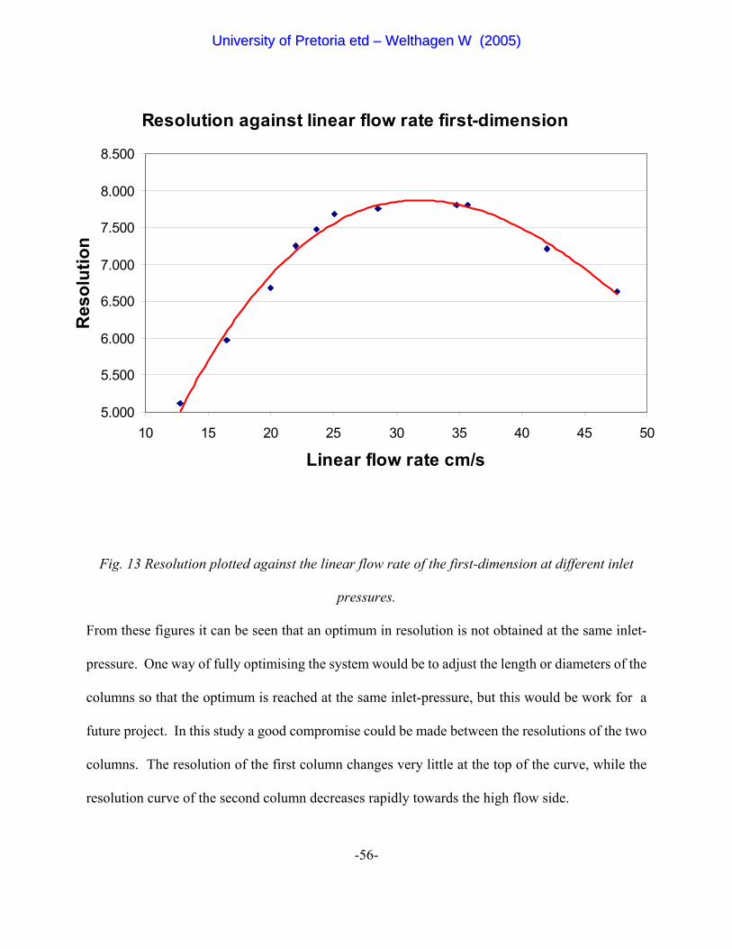
Fig. 13 Resolution plotted against the linear flow rate of the first-dimension at different inlet

pressures.

From these figures it can be seen that an optimum in resolution is not obtained at the same inlet-

pressure. One way of fully optimising the system would be to adjust the length or diameters of the

columns so that the optimum is reached at the same inlet-pressure, but this would be work for a

future project. In this study a good compromise could be made between the resolutions of the two

columns. The resolution of the first column changes very little at the top of the curve, while the

resolution curve of the second column decreases rapidly towards the high flow side.


-57-

Resolution against linear flow second-dimension

1

1.2

1.4

1.6

1.8

2

2.2

2.4

2.6

100 150 200 250 300 350 400 450

Linear flow rate cm/s

Res

olut

ion

Fig. 14 Resolution plotted against the linear flow rate of the second-dimension at different inlet

pressures.

It was thus decided to run the first-dimension at a slightly slower and the second-dimension slightly

faster than their respective optimum flow rates. The inlet-pressure corresponding to this point was

110 kPa and provides 88% of the optimum resolution in the first-dimension and 90% of the optimum

resolution in the second-dimension.


-58-

Resolution against system inlet pressure

0.0

1.0

2.0

3.0

4.0

5.0

6.0

7.0

8.0

9.0

60 80 100 120 140 160 180 200 220Inlet pressure kPa

Res

olut

ion

First-dimensionSecond-dimension

Fig. 15 Plot of resolution of the first- and second-dimension against the system inlet pressure (the

absolute resolution values of the second-dimension are adjusted by a factor of 3.20 for better visual

comparison).

The reason for using this resolution determination rather than the Van Deemter plot in the flow

optimisation study should be highlighted at this point:

1) Although the Van Deemter plots would be the more conventional/ theoretical approach it would

require isothermal operation of both columns (constant k-values required for N and H calculations)


-59-

which is difficult to achieve in practise.

2) Resolution determinations are just as valid under the more practical temperature programming

conditions and do not require the determination of absolute retention times, which are not easily

obtained in the GCxGC system used in this study.

3) Referring to the resolution equation (see Chapter 3): Provided the α- and k-values for the two

peaks used do not change appreciably with flow rate, the resolution achieved will be directly related

to the plate number and plate height. Flow optimisation of the resolution method under these

circumstances would then be equivalent to plate height optimisation (Van Deemter plot)

4) In any event resolution optimisation as performed in this GCxGC study has more practical

importance, as it incorporates both columns and modulator performance.

This resolution optimisation strategy should, however, not be done without investigating potential

errors of interpretation. In this study a fixed temperature program in the first dimension was used.

This would result in the compounds used for the calculations eluting at slightly different

temperatures (and k-values) with the change in flow rate. The first-dimension elution temperature

is also of concern for the retention behaviour of the second column since the analysed compounds

are subsequently subjected to slightly different second-dimension column temperatures under

different flow rates. This variation in temperatures would slightly affect the k-values and possibly

the α-values with consequences on resolution as predicted by the resolution equation (Chapter 3),

but unrelated to the flow rates. Compounds of similar chemical nature were therefore chosen for

the calculations since these compounds do not produce significant changes in α-values with

temperature. The changes in α- and k-values with flow would both introduce changes to the


-60-

resolution (R) values that are test compound related but not column performance (N) related, i.e.

cannot be ascribed to changes in longitudinal diffusion or slow radial equilibria. The slow

temperature program chosen in the first-dimension produces large elution k-values (the lowest k

values for a particular compound occur at their highest temperature in the column, i.e. at elution)

such that the k/(k+1) term approaches unity as depicted in Figure 10 (Chapter 3). Thus only slight

changes in α are likely to contribute to changes in resolution with flow rate in the first-dimension -

an effect suppressed by selecting two peaks that are chemically very similar, so that their relative

k values do not change much with temperature.

This is not true for the second-dimension, as fast GC is often performed at very small k-values (k

< 4). This more critical case is therefore dealt with in greater detail below:

In Tables 5 and 6 the k- and α-terms of the test compounds are calculated for the respective column

head pressures used. This requires determination of absolute retention times and linear flow rate.

In practise this is not done that easily as there is no trigger for the beginning of second-dimension

chromatograms and the absolute retention times of peaks are thus uncertain. This was also one of

the major considerations for using the more practical resolution approach since in this method only

relative retention times are required. With the calculated “dead time” (section 5.3.1) the absolute

retention times of the test compounds can be calculated. This was done by firstly adjusting the two-

dimensional contour plot so that the unretained compounds from the second-dimension (low boiling,

non polar compounds, i.e. the C3 and C4 alkanes) are on the zero position of the time axis. The

“dead time” is then added to this zero position to give absolute retention times.


-61-

Table 6 The k - values and k - term used in the resolution equation

Inlet Pressure Peak 1 Peak 2

k - values k / (k + 1) k - values k / (k + 1)

60

80

90

100

110

120

130

150

190

2.497

2.834

3.050

3.188

3.371

3.422

3.936

4.333

5.641

0.714

0.739

0.753

0.761

0.771

0.774

0.797

0.813

0.849

2.896

3.280

3.540

3.714

3.922

3.984

4.532

5.000

6.401

0.743

0.766

0.780

0.788

0.797

0.799

0.819

0.833

0.865

Table 7 The α - values and α - term used in the

resolution equation

Inlet Pressure α - values (α - 1) / α

60

80

90

100

110

120

130

150

190

1.160

1.157

1.161

1.165

1.164

1.164

1.151

1.154

1.135

0.138

0.136

0.138

0.142

0.141

0.141

0.131

0.133

0.119


-62-

As predicted the k-values (Table 6)are rather small and hence the k-term of the resolution equation

could vary a lot, but at the region of resolution optimum (i.e. 90 - 120 kPa) the k-term deviated

within a 2% (7% over the whole range measured). The α-terms (Table 7) have an even lower

deviation of only 2% over the total head-pressure range measured.

Whereas the resolution values (R) are also affected by the retention factors (k) and α value for the

test compounds, N values depend only the column performance as measured by N = (tr/σ)2.

Resolution values can be converted to N values once the k and α values of the test substances are

known. By rearrangement of the well known resolution equation (Chapter 3) we obtain:

N Rk

k=

+⎛⎝⎜

⎞⎠⎟ −⎛⎝⎜

⎞⎠⎟4

11

2 αα

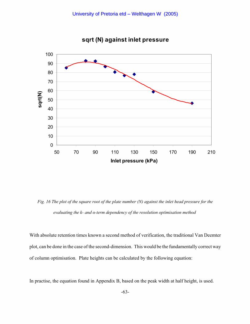
The square root N values, thus calculated and presented in Figure 16, show that for our set of

second-dimension peaks (k •3), the optimisation in resolution and in column performance is found

at much the same inlet pressure/ linear flow rate. (Note that the optimum N value is found at a

marginally higher flow rate - justification for our theoretical concern over k and α values.) This

means that flow optimisation of the R value for the selected pair of compounds does indeed optimise

N values or column performance, obviating the need for the much more involved calculation of N

values that require absolute retention times.


-63-

sqrt (N) against inlet pressure

0

10

20

30

40

50

60

70

80

90

100

50 70 90 110 130 150 170 190 210

Inlet pressure (kPa)

sqrt

(N)

Fig. 16 The plot of the square root of the plate number (N) against the inlet head pressure for the

evaluating the k- and α-term dependency of the resolution optimisation method

With absolute retention times known a second method of verification, the traditional Van Deemter

plot, can be done in the case of the second-dimension. This would be the fundamentally correct way

of column optimisation. Plate heights can be calculated by the following equation:

In practise, the equation found in Appendix B, based on the peak width at half height, is used.


-64-

Van Deemter Plot of two second-dimension retention peaks

0

0.01

0.02

0.03

0.04

0.05

0.06

0.07

0 100 200 300 400 500

Linear flow rate (cm/s)

Plat

e he

ight

H

Fig. 17 The plate height for the two peaks used in the resolution calculations is calculated and

plotted against the linear velocity of the second-dimension to give Van Deemter plots of the

second-dimension.

From figure 17 it is clear that the optimum determined in the resolution approach is the same as the

square root N and Van Deemter optimum in the graph, i.e. 200 cm/s. The minimum plate height

obtained in this way is also a good indicator for evaluating the efficiency of the modulator injection.


-65-

The Van Deemter plot shows a much steeper gradient of the curve in the fast linear flow rate region

than what is expected for a 100 Fm column (see figure 11). Together with the minimum plate height

that is about 35% higher than theoretically predicted for the 100 Fm i.d. column, this indicates that

the modulator injection into the second-dimension still has a negative contribution to overall system

performance. This contribution (σi) has an enhanced effect at higher flow rates, where compounds

elute with narrower peaks in time.

[22]HLN

Lt

t

r= =

⎛⎝⎜

⎞⎠⎟

σ2

[16]σ σ σt col inj2 2 2= +

This would result in larger H values at higher flow rates (lower tr) as σt/tr will increase. The result

is a steeper flow dependant curve than expected from pure column considerations. Indeed it can be

speculated that σinj could even increase with flow rate due to cooling effect of the higher internal

carrier gas flow.

The result of the flow optimisation study shows up the danger of blindly using literature Van

Deemter [52,53] results or generally accepted optimum flow rates for a specific inner diameter

column.

In figure 18 a comparison of using the generally accepted linear flow rate (40 cm/s) and the new

recommended linear flow rate (22 cm/s). From the two diesel chromatograms in figure 18, it is


-66-

obvious that there is a much better separation in the resolution-optimised chromatogram and that

there is even “baseline” separation of compounds previously overlapping (compounds circled in

red).

To summarise: this study indicates that the resolution vs inlet pressure curves (Figure 15) for both

dimensions are sufficient for GC x GC flow optimisation. It obviates the need to determine absolute

retention times and linear flow rates. The more involved Van Deemter optimisation for the second-

dimension does, however, give added information as to modulator performance.


-67-

R = 0.99

18

20

22

24

26

28

301 1.5 2 2.5 3

Second-dimension (s)

Firs

t-dim

ensi

on (m

in)

53 Peaks

Extract of a diesel chromatogram with linear flow rate of 40 cm/s

R = 1.77

22

24

26

28

30

32

341.2 1.7 2.2 2.7 3.2


Firs

t-dim

ensi

on (m

in)

68 Peaks


R = 0.99

18

20

22

24

26

28

301 1.5 2 2.5 3


Firs

t-dim

ensi

on (m

in)

53 Peaks


R = 1.77

22

24

26

28

30

32

341.2 1.7 2.2 2.7 3.2


Firs

t-dim

ensi

on (m

in)

68 Peaks


Fig. 18 A comparison between diesel chromatograms using the generally accepted linear flow

rate of 40 cm/s for the first-dimension and the optimised linear flow rate of 22 cm/s.


-68-

5.3.3 Choice of second dimension stationary phase

The choice of a stationary phase in chromatographic separations generally depends on the type of

separations required and the type of sample to be analysed (see discussion on dimensionality

Chapter 2). As discussed in Chapter 3 the two different stationary phases used in this study were

a PEG column and 17% cyanopropylphenyl - 83% dimethyl polysiloxane column. The PEG column

which is quite a polar column is in principle the best phase to provide “polarity” separation (see

orthogonality consideration Chapter 2). The PEG column can separate compounds of different

polarity with great efficiency, but the time required to separate these compounds becomes

increasingly long as the polarity range of compounds in a sample increases. The second-dimension,

however, has a limited time allowed for the compounds to elute. For the most polar compounds to

elute within the fixed time frame (modulation period) the column is run at higher temperatures,

which result in compounds eluting early in the chromatogram to be “squashed” together (lower R

values at too low k values). This behaviour is referred to as the general elution problem (section

3.2.4). In principle, temperature programming in the second-dimension will solve this problem; a

technology not yet available for the fast, repetitive second-dimension. Presently the PEG column

is probably best reserved for samples containing compounds in a narrow polarity range.

The use of a less polar column like the 17% cyanopropylphenyl - 83% dimethyl polysiloxane

column allows a lower temperature separation and decreased “squashing” of early eluting peaks.

The separation of different polarity classes obtained with this column is less than that of the PEG

column. The 17% cyanopropylphenyl - 83% dimethyl polysiloxane column can, however, separate


-69-

compounds eluting early (i.e. alkanes and cycloalkanes) in the chromatogram much more efficiently.

The eventual aim of this study was to investigate potential applications for the analysis of diesel

samples, which contain mostly compounds of low polarity alkanes and cyclic alkanes, as well as

some medium polar (mono-aromatic, di-aromatic and tri-aromatic) compounds.. The 17%

cyanopropylphenyl - 83% dimethyl polysiloxane column proved to be more robust in that it seemed

to have a much longer life time than the PEG column. Both columns had an upper temperature limit

of 270EC but the PEG column required operation at or above its recommended maximum

temperature when diesel samples were analysed at higher temperatures (higher temperatures to get

the compounds to elude in the defined modulation period). The 17% cyanopropylphenyl - 83%

dimethyl polysiloxane column was, therefore, the column of choice in this optimisation study.

In figure 19 a comparison between the two different columns can be seen. From these figures some

of the above concerns for not using the PEG becomes more apparent. In the accompanying

extraction sections of the figures it can be clearly seen that the PEG column is able to separate

compounds with great efficiency, but can do so only in specific narrow polarity ranges (in the case

presented here it was best suited for separating the aromatic bands and thus the alkane and cyclo-

alkane bands is “squashed” together, small k-values), the cyanopropylphenyl column on the other

hand provides a more even separation of all the compound groups analysed (k-values bigger than

three).


0

25

50

75

100

125

150

175

200

225

0 1 2 3 4 5 6Second-dimension (seconds)

Firs

t-dim

ensi

on (m

inut

es)

Diesel analysed on a PEG column

Extraction

262

3

4

5

6

7

8

A

27

9

10

11

12

13

14

15

16

17

18

1920

2122

2324

30

31

2829

Q

R

B

C

D

E

F

G

HI

J

K

L

M

N

O

P

ab c

d

ef

g

h

0

25

50

75

100

125

150

175

200

225


Firs

t-dim

ensi

on (m

inut

es)


Extraction

262

3

4

5

6

7

8

A

27

9

10

11

12

13

14

15

16

17

18

1920

2122

2324

30

31

2829

Q

R

B

C

D

E

F

G

HI

J

K

L

M

N

O

P

0

25

50

75

100

125

150

175

200

225


Firs

t-dim

ensi

on (m

inut

es)


Extraction

262

3

4

5

6

7

8

A

27

9

10

11

12

13

14

15

16

17

18

1920

2122

2324

30

31

2829

Q

R

B

C

D

E

F

G

HI

J

K

L

M

N

O

P

ab c

d

ef

g

h

Fig. 19a The chromatogram of a diesel sample analysed on a PEG second-dimension column


33

38

43

48

53

58

63

68


Firs

t-dim

ensi

on (m

inut

es)

Diesel analysed on a PEG column (2D extraction of Figure 19a)

C11

C12

C10

Naphthalene

Alk

anes

Cyc

lic a

lkan

es

mono-aromatics33

38

43

48

53

58

63

68


Firs

t-dim

ensi

on (m

inut

es)

Diesel analysed on a PEG column (2D extraction of Figure 19a)

C11

C12

C10

Naphthalene

Alk

anes

Cyc

lic a

lkan

es

mono-aromatics


0

25

50

75

100

125

150

175

200

225


Firs

t-dim

ensi

on (m

inut

es)

Diesel analysed on a cyanopropylphenyl column

50

75

Extraction

25262

3

4

5

6

7

8

A

27

1

9

10

11

12

13

14

15

16

17

18

19

2021

2223

24

30

31

2829

Q

R

S

T

B

C

D

E

F

G

H

I

J

K

L

M

N

O

P

ab cd

ef

h

0

25

50

75

100

125

150

175

200

225


Firs

t-dim

ensi

on (m

inut

es)


50

75

Extraction

25262

3

4

5

6

7

8

A

27

1

9

10

11

12

13

14

15

16

17

18

19

2021

2223

24

30

31

2829

Q

R

S

T

B

C

D

E

F

G

H

I

J

K

L

M

N

O

P

0

25

50

75

100

125

150

175

200

225


Firs

t-dim

ensi

on (m

inut

es)


50

75

Extraction

25262

3

4

5

6

7

8

A

27

1

9

10

11

12

13

14

15

16

17

18

19

2021

2223

24

30

31

2829

Q

R

S

T

B

C

D

E

F

G

H

I

J

K

L

M

N

O

P

ab cd

ef

h

Fig. 19b The chromatogram of a diesel sample analysed on a cyanopropylphenyl second-dimension column


33

38

43

48

53

58

63

68


Firs

t-dim

ensi

on (m

inut

es)

Diesel analysed on a cyanopropylphenyl column (2D extraction of Figure 19b)

Naphthalene

C11

C12

C10

Alk

anes

Cyc

lic a

lkan

es

mono-aromatics

33

38

43

48

53

58

63

68


Firs

t-dim

ensi

on (m

inut

es)

Diesel analysed on a cyanopropylphenyl column (2D extraction of Figure 19b)

Naphthalene

C11

C12

C10

Alk

anes

Cyc

lic a

lkan

es

mono-aromatics


-74-

Table 8 Names of peaks used in the diesel and paraffin chromatograms [17,55]

Individual compounds Some more identified compounds

123456789

10111213141516171819202122232425262728293031

n-C6n-C7n-C8n-C9n-C10n-C11n-C12n-C13n-C14n-C15n-C16n-C17n-C18n-C19n-C20n-C21n-C22n-C23n-C24n-C25n-C26n-C27n-C28n-C29BenzeneTolueneNaphthalenePhenanthreneAnthracenePristanePhytane

abcdefgh

ethylbenzenemeta + para-xyleneortho-xyleneisopropylbenzene2-methylnaphthalene1-methylnaphthalenebi-phenylfluorene

Grouped compounds

ABCDEFGHIJKLMNOPQRST

(CHx)2-benzene(CHx)3-benzene(CHx)4-benzene(CHx)5-benzene(CHx)6-benzene(CHx)7-benzene(CHx)8-benzene(CHx)9-benzene(CHx)10-benzene(CHx)11-benzene(CHx)1-naphthalene(CHx)2-naphthalene(CHx)3-naphthalene(CHx)4-naphthalene(CHx)5-naphthalene(CHx)6-naphthalene(CHx)1-anthracene or (CHx)1-phenanthrene (CHx)2-anthracene or (CHx)2-phenanthrene(CHx)3-anthracene or (CHx)3-phenanthrene(CHx)4-anthracene or (CHx)4-phenanthrene


-75-

5.3.4 Temperature difference between the columns

From section 5.3.3 it is obvious that there are specific temperatures required for fast second-

dimension separation. The second-dimension is operated at a constant temperature difference with

the first-dimension temperature. The temperature difference depends on the sample used, the

dimensions and the stationary-phase of the second-dimension column. In our case we never changed

the column dimensions. The optimisation of the temperature difference has to take the following

into consideration: The modulation period (time allowed for each second-dimension chromatogram)

is predefined by the temperature program of the first-dimension as this will dictate the time-width

of the peaks eluting from the first-dimension. This first-dimension peak has to be analysed several

times by the second-dimension column, a generally accepted number of cuts being four over each

first-dimension peak. For a temperature program of 1EC/min, providing ca. 30 s first-dimension

peak widths, the preferred second-dimension time is five to six seconds.

The temperature of the second-dimension column now needs to be adjusted in order to fully utilise

this predefined time. The temperature thus needs to be low enough to allow the compounds to

separate, but high enough (large enough k value, see Figure 10) not to stay in the column too long

to co-elute with the next second-dimension portion (“wrap-around”, figure 20). The temperature

should be selected for the peaks to elute over the full separation time. For the PEG column the

optimum temperature difference when analysing diesel was observed to be 30EC and that of the 17%

cyanopropylphenyl - 83% dimethyl polysiloxane column to be 20EC higher than the first-dimension

temperature.


-76-

Fig. 20 The peaks circled in red on the left of the picture represent second-dimension eluents

that overlap with those of the next second-dimension run. This phenomenon is called “wrap-

around”

5.4 Modulator optimisation

The modulator used in this study is a prototype and great care has to be taken in the operation and

maintenance thereof. The most critical factor in operating a GC x GC is for the second-dimension

injections to be very sharp and reproducible. It was observed that the peak sharpness can be

increased by using shorter heat pulse times, but this needs to be monitored very closely as too short


-77-

heat pulses can cause inefficient heating of the cold spots. In figure 21 the result of too short or too

long heat pulses can be seen.

Fig. 21 Actual peak profiles obtained with adjustment of the heat pulses, top figure indicating a

good peak shape (60-180 ms heat pulse), the middle one a too short heat pulse (smaller than 60

ms) and the last one a too long heat pulse (longer than 180 ms).


-78-

The step that is formed in the middle chromatogram (behind the short heat pulse peak) indicates that

not all of the eluent trapped on the cold spot is injected at once and the rest is injected in a delayed

step. The sharp decline at the end of the step indicates that the cold jet has been reactivated and is

cooling the spot down, trapping the remainder of the eluent that should have been injected if the

pulse was of sufficient heat. The too long heat pulse has a similar effect but now unmodulated

eluents from the first-dimension column are starting to move through the trap due to the trap being

too warm for the cold jets to trap this eluent. The sharpest peak shapes were found when using a

heat pulse of between 60 ms and 180 ms. The longer pulse was chosen due to some weather related

effects discussed later.

The effect of using an increased gas pulse pressure was also examined. The increase of the gas

pressure in the hot jets worked effectively at oven temperatures below 150EC but at higher oven

temperatures the results were negatively affected. The negative effect was due to a too short heating

section in the modulator for the larger volume hot pulses and thus resulting in pulsing cooler gas

onto the cold spot than required to remobilise the trapped compounds. The last portion of the hot

pulse volume comes from outside the GC oven and indeed cools the trapped area too below the oven

temperature. As a modification to the modulator it would therefore be advised to use a longer

heating section (e.g. an additional 0.5 m of a metal tube being inside the oven) so that a larger

amount of hot gas can be blown onto the cold spot in a shorter time-frame.

During a period of high humidity in the laboratory it was noticed that the cold spots would condense

water from the atmosphere and cause ice formation. The ice collecting on the column has a much

higher thermal capacity, resulting in the heat pulses being inefficient in remobilising the eluents


-79-

trapped in the cold zones. This inefficiency ranged from increased peak widths to permanent

trapping of eluents. In a first attempt to reduce this effect, a lower cold flow pressure was used to

just trap any first column eluents. This reduction in cold flow rates worked quite well at higher oven

temperatures, but at lower temperatures it was ineffective in trapping the more volatile eluents. To

utilise these reduced cold flow rates, different flow stages thus had to be defined for the cold flow.

At temperatures below 10EC a cold flow of above 40 ml/min is needed, between 10EC and 40EC

a flow of 30 ml/min was effective and above 40EC the cold flow can be reduced to 20 or 15 ml/min.

The reduced cold flow rates helped a lot in decreasing ice formation above 40EC but at lower

temperatures other precautions had to be taken: The oven was cryogenically cooled to 10EC and

lower with liquid nitrogen, to reduce the water content of the oven atmosphere. As the liquid

nitrogen evaporates it displaces the humid atmospheric air from the GC oven. In normal cool down

mode the oven vents open for faster cooling with laboratory air, also during the initial stages of the

GC run when the cold jets of the modulator start to operate and freeze out laboratory moisture on

the cold spots of the modulator. As a further precaution silica gel was placed inside the oven and

the oven vents were sealed with aluminium foil to keep the moisture levels down during instrument-

down periods. These precaution measures have shown great improvement in modulator operation,

in that the cold spots did not freeze up under these conditions, and that even lower flows (about 10

ml/min, compared to 20 ml/min without the precautions) of cold nitrogen air were required to

efficiently trap the compounds eluting from the first-dimension column. From a cost point of view,

this is of course, a great improvement.


optimisation of gc x gc parameters table of contents

Documents