Universita di Pisa

Dipartimento di Informatica

Technical Report

Optimization Methods: anApplications-Oriented Primer

Antonio FrangioniDipartimento di Informatica, Universita di Pisa

Largo B.Pontecorvo 3, 56127 Pisa, Italia, frangio@di.unipi.it

Laura GalliDipartimento di Informatica, Universita di Pisa

Largo B.Pontecorvo 3, 56127 Pisa, Italia, laura.galli@unipi.it

LICENSE: Creative Commons: Attribution – Noncommercial – No Derivative Works

ADDRESS: Largo B. Pontecorvo 3, 56127 Pisa, Italy. TEL: +39 050 2212700 FAX: +39 050 2212726

Optimization Methods: an Applications-Oriented Primer

Antonio FrangioniDipartimento di Informatica, Universita di Pisa

Largo B.Pontecorvo 3, 56127 Pisa, Italia, frangio@di.unipi.it

Laura GalliDipartimento di Informatica, Universita di Pisa

Largo B.Pontecorvo 3, 56127 Pisa, Italia, laura.galli@unipi.it

Abstract

Effectively sharing resources requires solving complex decision problems. This requires construct-ing a mathematical model of the underlying system, and then applying appropriate mathematicalmethods to find an optimal solution of the model, which is ultimately translated into actual decisions.The development of mathematical tools for solving optimization problems dates back to Newton andLeibniz, but it has tremendously accelerated since the advent of digital computers. Today, optimiza-tion is an inter-disciplinary subject, lying at the interface between management science, computerscience, mathematics and engineering. This chapter offers an introduction to the main theoretical andsoftware tools that are nowadays available to practitioners to solve the kind of optimization problemsthat are more likely to be encountered in the context of this book. Using, as a case study, a simplifiedversion of the bike sharing problem, we guide the reader through the discussion of modelling andalgorithmic issues, concentrating on methods for solving optimization problems to proven optimality.

Keywords: Optimization methods, combinatorial optimization, integer programming, bike sharing

1 Introduction

Effectively sharing resources is a complex task. A benefit of having dedicated resources (say, a personalcar) for a given task is that there is no need to take complex decisions about their use, as they arealways available. The obvious drawback is that they can be heavily under-utilized, thereby substantiallydecreasing their value while consuming other valuable resources (say, scarce parking space). Allowinga resource to be shared may dramatically increase its social and economic value, but it also opensup a number of complex issues regarding its fair and efficient management that need to be solved forthe system to deliver its potential benefits. Besides the many technological aspects (say, self-drivingcapabilities, accurate navigation, reliable communication, . . . ) that are crucial to make sharing possible,the ability of taking optimal decisions about highly complex systems (say, a large fleet of self-drivingcars) is also a fundamental pre-requisite for the sharing economy to thrive.

Many, although not necessarily all, of the decision procedures can be cast under the form of opti-mization problems, where one objective function depending on the decision variables has to be optimized(minimize the effort or maximize the benefit) along all possible states of the system, typically representedvia constraints. Problems of this kind are pervasive and can be found e.g. in design of structures andtrajectories, production planning, resource allocation, scheduling, control, and many others. The devel-opment of mathematical and software tools for the solution of these problems is a highly inter-disciplinarybranch of applied mathematics lying at the interface with diverse other subjects, including (but not lim-ited to) management science, computer science, and engineering, and is often generally referred to asOperations Research (OR). At its heart, OR is based on mathematical techniques that can be traced

1

back to Newton and Leibniz, and that have seen a tremendous development since the second half of lastcentury together with the meteoric rise of availability of computational power. This is indeed relevant, asoptimization problems are generally “difficult”. Without going into the mathematical details, suffices hereto say that the worst-case computational cost of the best known algorithms for solving most optimizationproblems grows extremely rapidly (exponentially) with the size of the problem, and not just in theory:the increase in complexity often shows off in practice. This motivated an enormous effort to develop effi-cient (as much as possible) algorithms for different classes of problems, exploiting all available structurethat each one has. The result is a complex panorama of many different classes of optimization problems:for instance, it is customary to distinguish between continuous optimization where decision variables cantake, say, real values, combinatorial optimization where solutions belong to some combinatorial space(sets, paths, trees, . . . ) (a.k.a. discrete optimization since usually decision variables are restricted to onlyattain discrete values), and functional optimization (a.k.a. optimal control) where solutions are func-tions. Each of these classes typically requires different mathematical tools to be addressed (say, analysisfor continuous and functional optimization and combinatorics for combinatorial optimization), althoughin practice the boundaries are blurred, and efficient optimization methods typically borrow from severaldifferent areas of mathematics and computer science.

Using mathematical optimization in practice is therefore a complex task that requires navigatingnontrivial trade-offs. The process typically starts by constructing a mathematical model trying to capturethe “essence” of one’s practical system to be managed. However, the model should attain the rightcompromise between correctly representing the reality at hand, and admitting “sufficiently efficient”algorithms that can provide the desired solutions in a time compatible with the constraints that theactual use case imposes (which can be rather tight). Therefore, a crucial decision while developinga mathematical optimization model is what class of optimization problems one selects to express themodel into, since this dictates what (mathematical, hence algorithmic and ultimately software) tools onehas at disposal to actually solve it, and therefore the chances to obtain a practical system. Indeed, it isone of the most important cultural legacies of the last century—from Godel’s incompleteness theoremsto the discovery of non-computable functions down to complexity theory—that just being able to writea mathematical model of one’s system does not imply that solutions can actually be found. Thus, usingoptimization methods requires in principle some understanding of the several “core techniques” thathave been developed to tackle different kind of problems, such as linear, non-linear, combinatorial andstochastic optimization, calculus of variations, optimal control, game theory, and several others.

However, for problems in contexts like the one of this book, the choices are typically limited. In fact,the problems are usually large-scale (thousands to hundreds of thousands of decision variables), withrather complex constraints encompassing both discrete and continuous decisions. In order to have anychance of solving problems of this type, in most cases one has to restrict to the class of Mixed IntegerLinear Programs (MILP), which only allows linear relationships between decision variables, therebyforcing to use somehow un-natural constructs for modelling certain relationships. However, the classis expressive enough to allow to represent very many systems, and the vast majority of optimizationmodels in the applications of interest for this book (logistics, transportation, telecommunications, . . . )are customarily written as MILP. Furthermore, many software tools are currently available for solvingthis class of problems. Which does not mean that MILP are not “difficult” problems: in general, thecomplexity of algorithms for their (exact) solution is exponential. However, due to more than 70 years ofcontinuous research by a large community, the current status of solution algorithms for MILP is such thatfor several practical problems, just writing the MILP model and passing it to a solver may be enough toobtain solutions with a “reasonable” computational effort. Although there is no guarantee that this willhappen for any specific application, the effort for testing this approach is low enough that most oftenthis is the first step that should be attempted (unless perhaps if the problem is extremely-large scale, orneeds to be solved in extremely short time, or has many complex nonlinear relationships); with any luck,it may also be the only step that is needed.

In this chapter, after an introduction about general optimization models in Section 2 we will thereforeconcentrate on MILP. The concepts will be illustrated by means of a case study inspired by a bike sharingsystem, described in Section 3. In Section 4 we will concentrate on a crucial and nontrivial aspect, whichis that there are many possible ways to formulate the same system as a MILP model, and that this choice

2

is actually crucial for the effectiveness of the solution algorithms. Finally, in Section 5 we will providepointers for further reading on the subject.

2 Optimization problems

A quite general (although not the most general) optimization problem is

(P) min{ f(x) : G(x) ≤ 0 , xi ∈ Z i ∈ I } ,

where x = [x1 , . . . , xn ] is the (finite) vector of decision variables. When not otherwise specified, eachxi can attain real values, i.e., x ∈ Rn; this already restricts (P ) to a finite-dimensional space, therebyexcluding problems where xi may be, say, itself a function. The objective function f(x) and the (finitenumber of explicit) constraints G(x) = [ gj(x) ]j=1,...,m are usually assumed to be real-valued functions,i.e., f : Rn → R and G : Rn → Rm. For f , this implies that the decision-maker only has one objective,which is often not true in practice as there could be any number of—possibly, contrasting—measures tobe optimized. Yet, this is necessary to univocally define the concept of optimal solution; with a vector-valued f(x) = [ fh(x) ]h=1,...,k : Rn → Rk, the lack of a complete order in Rk (for k > 1) means that onehas rather to resort to the concept of nondominated (a.k.a. Pareto-optimal) solution, but this would meanthat (P ) does not identify one solution that can be automatically taken as the answer without humanoversight, as it is often necessary to do. Thus, in presence of multiple objective functions it is customaryto either form a weighted sum (f(x) =

∑h=1,...,k αhfh(x), a.k.a. weighting) or define thresholds on the

least acceptable value for all objectives save one (budgeting), and fall back to the single-objective case.Even so, f and G cannot clearly be just “any” function, as there are functions that simply cannot becomputed; in general, the assumption is that they are “easy” to compute, most often algebraic functions.Yet, even restricting (P ) to algebraic functions is not enough to tame its complexity: even with simplepolynomials, the problem may be undecidable (provably, for some instances there cannot be any solutionalgorithm). This justifies why it is customary to work with classes of optimization problems correspondingto restricting the shape of f and G. Indeed, by far the most common class of optimization problems forthe applications of interest here is that of Mixed-Integer Linear Programs (MILP), where both f and Gare linear ; that is,

(MILP) min{ cx : Ax ≤ b , xi ∈ Z i ∈ I } ,

where c ∈ Rn is the cost (row) vector, A ∈ Rm×n is the constraint matrix, b ∈ Rm is the (column) vectorof right-hand sides. This finally justifies why, besides the explicit constraints, (P ) also has integralityconstraints on a (possibly empty) subset I ⊆ N = { 1 , . . . , n } of the variables; although these could beexpressed in an algebraic way, doing so would require “complex” functions.

Even with such a dramatic restriction to the set of available functions, MILP is a “hard” problem.However, at least it is now “clear where the hardness comes from”: with no integrality constraints (I = ∅)the problem becomes a Linear Program (LP), which is instead “easy”. Formally, this means that there aresolution algorithms whose complexity grows at most as a polynomial (although, not a very low degree one)in the size of the problem. In practice, this means that LPs with up to hundreds of thousands of variablesand constraints can routinely be solved with standard approaches on standard PCs, and that LPs withup to billions of variables can be approached with appropriate techniques on HPC systems. As we shallsee in Section 4, this is a crucial property upon which all the available solution approaches to MILP rely.Indeed, the fact that LP admit “efficient” algorithms is the main reason why MILP is the most widelyused class of optimization problems: although MILPs are in general “hard”, formulating one’s problemin this shape allows to exploit the huge amount of research, and the many available actual softwareproducts, dedicated to their solution. The advances in those approaches over the last decades have beensuch that many practical problems, despite being theoretically “hard”, can nowadays be routinely solvedby just applying off-the-shelf technologies once they have been properly formulated as MILPs.

Yet, doing so is not straightforward, for two reasons. The first is that while MILP is a quite “expres-sive” class, in the sense that an enormous number of different relevant problems can be written as such,the severe restriction of being only able to use linear functions requires getting familiar with a number ofmodelling tricks, whereby the limitations of the framework are sidestepped by clever contraptions. The

3

second, and perhaps more important, is that there are usually very many different MILP formulationsof a given problem, which are typically not equivalent in terms of computational cost. Quite on thecontrary, writing the “right” MILP formulation of the problem can easily be the deciding factor in beingable to solve it, with orders-of-magnitude differences between apparently similar formulations being notuncommon. All in all, there is no systematic way to formulate an optimization problem as a MILP, anddevising a good model is often more of an art than of a science. However, some general guidelines can beprovided, which is what we will attempt in the rest of this chapter. In particular, the next section, usingone specific case study, will focus on the process of writing a MILP formulation out of the “informal”description of one’s situation. Then, in Section 4 we will very briefly summarize the main concept un-derlying the most effective (least ineffective) solution methods for MILP, as doing so allows to pinpointthe characteristics that a “good formulation” should ideally possess.

However, to conclude this section it is important to remark that MILP is not the most general class ofoptimization problems for which (relatively) efficient solution tools are available. Indeed, it is possible to“slightly” enlarge the set of functions available to express f andG while keeping a solution cost comparablewith that of a MILP of the same size. For instance, this is possible with Mixed-Integer QuadraticPrograms (MIQP) that have convex quadratic functions of the form f(x) = xTQx+qx, with Q a positive

semidefinite matrix. More in general, Second-Order Cone constraints of the form xn ≥√∑n−1

i=1 x2i can

be used as well; a surprising number of different nonlinear functions can be formulated as such, andthe best current software tools can usually handle Mixed-Integer Second-Order Cone Programs (MI-SOCP) efficiently. Even Mixed-Integer Nonlinear Programs (MINLP) with general convex functions canbe tackled with similar approaches, although with a somehow lower efficiency. Finally, there are toolscapable of solving (or attempting to) MINLP where f and G are general algebraic or transcendentalfunctions; however, their efficiency in practice can easily be orders of magnitude lower than those forMILP problems of comparable size. All in all, the best course of action when devising a mathematicalmodel is most often to start with a MILP one, unless perhaps if the practical problem have either complexnonlinear relationships that cannot reasonably be simplified, or simple nonlinear relationships that can beexpressed within the classes of functions that make MINLPs “not too much more difficult” than MILPs.

3 Case Study: the bike sharing problem

Bike Sharing (BS) is an urban mobility service that makes public bicycles available for shared use. Thebicycles are located at some stations distributed across the urban area. Customers can take a bicycle fromone of the stations, use it for a journey, then leave it at a possibly different station, paying according tothe time of usage. This is an important service in green logistics, in that on one hand it helps to decreasetraffic and CO2 emissions, and on the other hand it offers a partial solution to the so-called “last mileproblem” related to proximity travels.

The cost of operating a BS system has several components: the setup costs (i.e., buying and installingstations and bikes), the cost of the back-end system to operate the equipment, and daily operatingcosts like maintenance, insurance, and the cost of redistributing bikes among the stations. Ideally, thisbeing a “system” one should optimize all its aspects symulteneously; however, in practice this is usuallyimpossible. For once, different costs are incurred at different times: setup costs are paid once, beforethe system can start operating, and the consequences of the corresponding strategic decisions affect theday-to-day operations for a long period. Instead, operating decisions such as how many bikes shouldbe moved from one station to another can only be taken after the particular situation of a given day isknown. Taking all these decisions in one step is impossible, due both to lack of data about the future andto the fact that that the corresponding optimization problem would be so huge as to being intractable.Therefore, it is crucial to devise the right trade-off between system model tractability and accuracy.

In practice, optimization of a complex system is usually decomposed into independent sub-problems,where independence comes either from considering different time horizons (strategic vs. operational deci-sions), or from purposely ignoring present but sufficiently “weak” dependencies, say by approximating theeffect of the choices in one subproblem on the others’ feasibility and cost. Besides making the problemseasier to solve, this usually leads to the discovery that each of the sub-problems has strong similarities

4

with other known problems, coming from similar or even completely different settings. This is why the ORliterature often focuses on classes of “abstract” models (say, Vehicle Routing models, Location models,. . . ) that represent common mathematical structures that appear in many different real-world contexts,possibly as sub-problems or with variants. Once one’s problem has been identified, it is therefore usuallypossible to find similar cases in the literature, which can greatly help in devising a good (MILP) model.

Our case study gives rise to several optimization sub-problems such as: bike station location and fleetdimensioning, allocation of bikes to stations, re-balancing incentives setting, and bike repositioning. Wewill concentrate on the latter, that represents one of the main daily operating costs, with a consistentimpact on the budget. In fact, even if in the early morning all the bike stations meet the desired level ofoccupation, due to the users’ travel behaviour in the evening some stations are typically full and others areempty. Repositioning is crucial in order to offer a good service all day long, and is usually done by meansof capacitated vehicles, based at a central depot, that pick up some bicycles from the stations where thelevel of occupation is too high and deliver them to those stations where the level is too low. The depotalso keeps a buffer of bicycles to allow a more flexible redistribution. Driving the vehicles around theurban area is expensive, thus one needs to decide how to route the vehicles to perform the redistributionat minimum cost. This optimization problem is known as the Bike sharing Re-balancing Problem (BRP),and has recently received considerable attention from both the OR community and practitioners in thearea. We will only consider the static version in which the occupancy of each station is considered fixed,as this corresponds to the heavier re-balancing operations performed at night when the system is closedor demand is very low. A dynamic version exists where real-time usage information is taken into accountto update the redistribution plan even as the vehicles are performing it, but this requires more complexmodelling techniques to represent uncertainty of future events that are out of the scope of this simpletreatment.

3.1 BRP: system model

The first step to develop a mathematical model is to define the so-called system model, that describes theinvolved entities, their relations and the corresponding parameters. A system model is usually definedalready as much as possible in terms of mathematical objects, and significant decisions are made as towhich entities and relations are significant, which ones are ignored, and which relations are simplified.

In the BRP case, the system consists of the depot, the vehicles, the stations, and the urban roadnetwork that connects them. This can be described using a complete directed graph G = (N,A), wherethe set of nodes N = {0, 1, . . . , n} contains the depot, node 0, and the stations, nodes N ′ = {1, 2, ..., n}.An arc (i, j) ∈ A represents the shortest path in the actual city road network connecting the locationscorresponding to the two nodes i and j, with the associated traveling cost cij . Since the BS system islocated in an urban area, where one-way streets often strongly affect the feasible paths, arcs (i, j) and(j, i) may have different costs. Each station node i has a request qi, which can be either positive ornegative: if qi > 0 then i is a pickup node, where qi bikes must be removed, while if qi < 0 then i is adelivery node, where −qi bikes must be supplied. The requests are computed as the difference betweenthe number of bikes present at station i when performing the redistribution and the desired number ofbikes in the station in the final configuration. This is a typical example of a link between two decisionphases: the desired number of bikes is established during the planning phase, where re-distribution costsare estimated without taking into account detailed routing choices (e.g., by some average), and then takenas a constraint in the operational phase. A fleet of m identical vehicles, each with capacity Q (bikes), islocated at the depot. The bikes removed from pickup nodes can either go to a delivery node or back tothe depot, and similarly for those supplied to delivery nodes.

The problem is to decide how to route at most m vehicles through the graph, with the objective ofminimizing the total traveling cost while satisfying the following constraints:

1. each vehicle performs a route that starts and ends at the depot;

2. each station is visited exactly once, which implies that its request is completely fulfilled by the onevehicle visiting it;

5

3. each vehicle starts from the depot with some initial load, comprised between 0 (empty) and Q(full), and the vehicle load at each step of the route, corresponding to the the sum of requests ofthe visited stations plus the initial load, is never negative or greater than Q.

In setting the system model, some important decisions have already been taken. For instance, it mightbe possible to serve a station with more than one vehicle, each satisfying a fraction of the demand. Thiswould enlarge the space of feasible BRP solutions, allowing more flexibility in the redistribution plan atthe cost of complicating the operational procedures; we assume that the operator has decided againstit, but a somehow different model could be developed to check the economical impact of the choice andperform what-if analysis. Also, we allow flow of bikes on the depot to be either positive or a negative,which is useful to model cases in which some bikes have to be brought back to the depot for maintenance,and then put in operations again. Finally, it is assumed that there is enough time available to perform allthe operations (although some routes can be “long”) and that stations can be serviced at any time; thisallows to completely ignore the exact moment at which each operation is performed, that may insteadbe a relevant information in other variants of the problem (e.g., the dynamic one).

3.2 BRP: MILP formulation

The second step is developing a MILP formulation. As it often happens, the model is closely related to awidely studied class of (difficult) combinatorial problems known in the literature as Capacitated VehicleRouting Problem (CVRP) [2, 3]. In particular, BRP is a Pickup and Delivery Vehicle Routing Problem(PDVRP). Thus, to define a MILP formulation one can use as a guide those that have already beenproposed in the literature.

A MILP model of BRP uses three types of decision variables:

• binary arc variables xij ∈ { 0 , 1 } taking value 1 if arc (i, j) is used by a vehicle (irrespectively towhich one), and 0 otherwise;

• non-negative continuous arc flow variables fij representing the current load of the vehicle travelingalong arc (i, j), if any;

• integer arc variables yij , representing the position of arc (i, j), if used, in the corresponding route.

The MILP model is the following:

min∑

(ij)∈A cijxij (1)∑(ij)∈A xij = 1 i ∈ N ′ (2)∑(ji)∈A xij = 1 i ∈ N ′ (3)∑(0j)∈A x0j ≤ m (4)∑(0j)∈A x0j −

∑(j0)∈A xj0 = 0 (5)∑

(ij)∈A fij −∑

(ji)∈A fji = qi i ∈ N ′ (6)

fijxij ≤ fij ≤ fijxij (i, j) ∈ A (7)∑(ji)∈A yji −

∑(ij)∈A yij = 1 i ∈ N ′ (8)

xij ≤ yij ≤ (n+ 1)xij (i, j) ∈ A (9)

xij ∈ { 0 , 1 } , yij ∈ N (i, j) ∈ A (10)

The objective function (1) minimizes the traveling cost. Constraints (2)–(3) ensure that each stationnode has exactly one incoming and one outgoing arc, while (4) and (5) ensure, respectively, that no morethan m routes (= vehicles) leave the depot, and that each leaving vehicle eventually returns. Next, flowconservation constraints (6) ensure that fij properly account for the number of bikes on the (single)

6

vehicle traversing arc (i, j). Then, (7) serve a double purpose. On one hand, when xij = 1, i.e., a vehicleis traversing arc (i, j), they guarantee that the load on a vehicle is feasible by imposing appropriate upperand lower bounds on it (for instance f

ij= max{ 0 , qi , −qj } and fij = min{Q , Q+ qi , Q− qj }, whose

validity can be easily verified with some reflection). On the other hand, when xij = 0 they guaranteethat fij = 0; hence, bikes can only “flow” on the graph following vehicles, as it is logically required. Onemay believe that these constraints (plus (10) dictating the binary nature of xij) be enough to correctlymodel the problem, but this is not so because they do not forbid sub-tours, i.e., closed oriented loops thatdo not include the depot. To picture this, consider two nodes i and j having qi = −qj > 0: it would betherefore possible to set xij = xji = 1, fij = qi and fji = 0, i.e., have a vehicle “appearing” at i, carryingall required bikes to j, getting back to i and “disappearing” there. Constraints (8)–(9), which are aversion of the so-called Miller-Tucker-Zemlin (MTZ) subtour elimination constraints originally devisedfor the Traveling Salesman Problem (TSP) [1], avoid sub-tours (of any length). The idea is to associatean ordering to the vertices of each route by assigning an integer “position” variable yij to each arc in theroute. Starting from the depot, the value of the position variables increases by one as we move to thenext arc along the route. Clearly, since a route is cyclic, we can impose an ordering for all the vertices inthe route except from the depot: indeed, (8) is not imposed for i = 0. Note that the maximum numberof arcs in a route is n + 1—a single route that visits all the vertices—yielding the upper bound on theposition variables.

Admittedly, devising such a formulation is not a trivial task. A number of formulation tricks havebeen used, such as extensive use of flow conservation constraints ((6), (8) and in fact even (2)–(5)) andconstraints imposing “logical” conditions, such as “xij = 0 =⇒ yij = 0, xij = 1 =⇒ yij ∈ [ 1 , n + 1 ]”((9), and similarly for (7)). Getting used to all the devious tricks necessary to devise a MILP formulationrequires some experience; however, as already recalled, most problems one encounters have very likelyalready been modeled, possibly with some variations, and therefore help is usually available. For instance,the MTZ constraints for the PDVRP are more complex than those for the CVRP where all goods originatefrom the depot; actually, in that case, the flow constraints (6) are sufficient to avoid sub-tours, as onecan easily see considering our counter-example above. Yet, the more complex version had already beendevised far before that BRP was ever conceived.

The advantage of formulating one’s problem as a MILP is that, once this is done, efficient (as muchas possible) software tools are available for (attempting to) solving it.

3.3 Software tools

Due to the huge number of practical applications leading to MILP models, there is no shortage of softwaretools for solving these problems. Actually, even forming the coefficient matrix A and the right-hand-sidevector b corresponding to a MILP is itself a nontrivial and error-prone task, especially considering thatpractical applications may originate even considerably more complex MILP models than (1)–(10). Thisis why software tools known as algebraic modelling languages are available to perform it, allowing todescribe one’s model in a way that is very similar to how equations are written in a document; theseequations are then processed to automatically construct the data of the problem (A, b, c, I). Several ofthese tools exist, both commercial ones such as AMPL [9] and GAMS [10], or open-source ones like Coliop

[11] and ZIMPL [12]. Also, modelling systems are available that implement similar functionalities withinmany different general-purpose programming languages, such as C++ (FlopC++ [13], COIN-Reharse [26]),python (PuLP [14], Pyomo [15]), Julia (JuMP [16]), Matlab (YALMIP [17]) and others. As an alternative,it is possible to construct the model by either writing a file with proper format (e.g., MPS [18] or LP[19]), or directly calling the in-memory API of the desired solver.

However the modelling phase is performed, the problem can then be solved using any of the severalavailable solvers, again both commercial ones like Cplex [20], GuRoBi [21], MOSEK [22] and others, oropen-source ones like Cbc [23] or SCIP [24]. The effectiveness of the solver should be expected to varyconsiderably; although all more or less based on the same ideas, quickly summarised in the next Section,implementation details may make an enormous difference on specific instances. Indeed, MILPs are“difficult”, and therefore one should in principle expect the problems to take a long time to solve; alarge set of sophisticated algorithmic techniques has been developed to try to improve on this, whose

7

implementation differs between different solvers. In general one should expect commercial solvers tobe more efficient than open-source ones (which justify the high licensing fees they usually require), butexceptions are not unheard-of. Indeed, all solvers have a large set of algorithmic parameters controllingtheir behaviour, whose appropriate tuning can make a very substantial difference.

Above all, however, choosing the right formulation is usually the most important factor dictating howefficiently the problem will ultimately be solved. To be able to at least introduce all this aspects, a veryquick recap of the algorithmic techniques that are employed is necessary.

4 Algorithmic approaches and “good formulations”

There are very many different algorithms for “hard” problems. In many practical applications, recognisingthe fact that efficiently finding provably optimal solutions is difficult, it is usual to resort to heuristics,i.e., algorithms that strive to efficiently provide “good” solutions, but give no guarantees on their quality.Most often heuristics are developed for a much more specific class of problems than MILP (say, PDVRP),although general frameworks for specific classes of heuristic approaches have been developed, such as localsearch, tabu search, simulated annealing, genetic algorithms and many others, and general-purpose solversexist (e.g. LocalSolver [25]). In some cases, approximation algorithms are available that provide explicita-priori bounds on the quality of the solution obtained within a given computational effort, but againthese strongly depend on the specific problem, and are not available for general MILP. In this section wewill rater concentrate on exact algorithms, that guarantee to find an optimal solution, albeit possibly ata computational cost that may grow exponentially fast with the size of the problem. In particular wewill (briefly) discuss the Branch-and-Bound (B&B) approach underlying all the general-purpose solversalluded to above, with its crucial variants known as Branch-and-Cut and Branch-and-Price.

These approaches are inherently based on the concept of relaxation to provide bounds on the optimalvalue of the problem. In general, a relaxation of an optimization problem (P) (assuming minimization)is another optimization problem (P′) such that: (i) its feasible set is larger than that of (P), and (ii)its objective function has the same or smaller value than that of (P) on the latter’s feasible solutions.By denoting as ν(·) the optimal value of an optimization problem, one clearly has ν(P′) ≤ ν(P). Thequestion then arises of how to construct interesting relaxations. However, as anticipated, the answer istrivial for (MILP), as one can simply use its continuous relaxation

(LP) min{ cx : Ax ≤ b } ,

i.e., the LP obtained by simply dropping the integrality constraints. It is immediate to realise that ν(LP)≤ ν(MILP), which may provide optimality conditions for a feasible solution x of (MILP). Indeed, considerthe (very fortunate) case in which the optimal solution x of (LP) satisfies the integrality constraints: itis immediate to realise that, in this case, cx = ν(LP) ≤ ν(MILP) ≤ cx. Thus, exploiting the efficientavailable LP algorithms we could, in principle, be able to not only find an optimal solution of the “difficult”(MILP), but also have a certificate of optimality proving it without any doubt. This actually hinges onbeing able to prove that x is optimal for (LP) in the first place, which typically relies on duality andultimately convexity of the problem, but we are not going to delve deeper in these concepts.

Unfortunately, in general ν(LP) < ν(MILP). Thus, besides bounding by relaxations some other mech-anism is required to ensure that the lower bound is increased and eventually reaches ν(MILP). Un-fortunately, the only (practical) general ways that have been devised for ensuring this are branching,a.k.a. (partial) enumeration, and cutting. Both are, for the best variants known so far, processes thatmay require an exponential number of iterations to achieve the desired results. Yet, they are also thebest (least worse) general-purpose available algorithms for MILP, hence what is used in practice. We willnow give a brief recount of their basic principles.

4.1 Branch-and-Bound

Branch-and-Bound (B&B) uses a “divide and conquer” approach to explore the set X of feasible solutionsof (MILP), as described in Algorithm 1. The idea is to partition X into a finite collection of subsets

8

X1, . . . , Xk and solve separately each one of the subproblems restricted to each Xi; one then comparesthe optimal solutions to the subproblems, and chooses the best one. However, since the subproblemsare usually almost as difficult as the original problem, it is typically necessary to solve each of themby recursively iterating the same approach, that is, splitting them into further subproblems. This is thebranching part of the method, which leads to a tree of subproblems T . Because X is typically exponentiallylarge, the B&B uses lower bounds on the optimal value of each subproblem to try to avoid exploring partsof it. These are obtained by solving the continuous relaxation. Actually, the corresponding (LP) mayhave no solution, which immediately implies that Xi has no integer solution as well; any LP solver canefficiently detect it, customarily returning ∞ as the optimal value and therefore allowing to fathom thecorresponding node of T by infeasibility. Otherwise, a continuous optimal solution xi is found that mayoccasionally be integer, in which case we can possibly have found a better upper bound on ν(MILP)than previously known, updating the incumbent value z (the cost of the best solution found thus far).The essence of the algorithm lies in the following observation: if the optimal value zi = cxi of thecontinuous relaxation of Xi satisfies zi ≥ z, then this subproblem need not be considered further, sincethe optimal solution of Xi is no better than the best feasible solution encountered thus far. In this case,the corresponding node of T can be fathomed by the bound ; it is immediate to realize that this surelyhappens if xi is integer, since then cxi ≥ z. Otherwise, branching has to occur, i.e., the current Xi isfurther split. Provided that the total number of subproblems that can be generated is finite, the B&Balgorithm clearly terminates in a finite (albeit, very possibly, exponentially large) number of iterationshaving correctly identified the optimal value z = ν(MILP). The incumbent solution having produced theincumbent value z is usually conserved as well, and at termination it is guaranteed to be an optimalsolution. Finiteness of the branching operation is usually trivial. For instance, if all variables are binary,the typical branching consists in selecting one variable in xi that has a fractional value and creating twosubproblems, in one of which the variable is fixed to 0, while in the other it is fixed to 1; a slightly moregeneral version is easily devised for integer variables. We remark in passing that branching for nonconvexMINLPs is a considerably more sophisticated process, justifying the higher practical cost of the latterw.r.t. MILPs.

Algorithm 1: Branch-and-Bound

Input: (MILP), subproblem-selection-rule, LP-relaxation, branching rule

Output: Optimal value z

1 Initialize T = {X }, z =∞2 while T 6= ∅ do3 Xi ← subproblem-selection-rule(T ) // select an active subproblem4 ( xi , zi )← LP-relaxation(Xi) // solve continuous relaxation5 if zi =∞ then6 delete Xi // subproblem Xi infeasible7 else8 if xi is feasible for (MILP) then9 z = min{ z , cxi } // new feasible solution found

10 if zi ≥ z then11 delete Xi // subproblem Xi fathomed by bound

12 else13 T ← branching rule(Xi)14 // break Xi into further subproblems and add them to T

15 end

16 end

17 end

Many aspects of the practical implementation of a B&B are potentially crucial, such as the exact choiceof the branching operation, the selection of the next active subproblem, and the details of the solutionof the continuous relaxation. Also, MILP solvers usually employ general-purpose heuristics which try

9

to generate feasible integer solutions, say by “cleverly” rounding the optimal continuous solutions xi.However, by far the most important factor dictating the effectiveness of a B&B is how often fathomingof a node (line 11) happens. This is clearly related to tightness of the lower bound, i.e., how close theoptimal value zi of the continuous relaxation is to the actual optimal value of Xi (although, of course,the quality of the upper bound z also is a factor). As a rule of thumb, MILPs for which zi is within avery few percentage points off the real value can be solved efficiently via the B&B, whereas if the relativegap is, say, above 10% then a huge number of nodes will be enumerated.

Crucially, this does not depend on the B&B solver, but rather on the quality of the formulation thatthe user has provided it. It is therefore important to explicitly define what the “quality” of a formulationis.

4.2 Strong, “large” formulations

For LP, a “good” formulation is one that has a small number of variables and constraints, because thecomputational cost of its solution depends (polynomially) on these. The situation for MILP is drasticallydifferent.

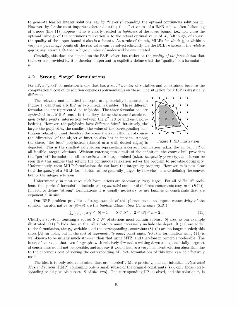
Figure 1: 2D illustration

The relevant mathematical concepts are pictorially illustrated inFigure 1, depicting a MILP in two integer variables. Three differentformulations are represented, as polyhedra. The three formulations areequivalent in a MILP sense, in that they define the same feasible re-gion (white points, intersection between the Z2 lattice and each poly-hedron). However, the polyhedra have different “size”; intuitively, thelarger the polyhedra, the smallest the value of the corresponding con-tinuous relaxation, and therefore the worse the gap, although of coursethe “direction” of the objective function also has an impact. Amongthe three, “the best” polyhedron (shaded area with dotted edges) isdepicted. This is the smallest polyhedron representing a correct formulation, a.k.a. the convex hull ofall feasible integer solutions. Without entering into details of the definition, the convex hull providersthe “perfect” formulation: all its vertices are integer-valued (a.k.a. integrality property), and it can beseen that this implies that solving the continuous relaxation solves the problem to provable optimality.Unfortunately, most MILP formulations do not have the integrality property. However, it is now clearthat the quality of a MILP formulation can be generally judged by how close it is to defining the convexhull of the integer solutions.

Unfortunately, in most cases such formulations are necessarily “very large”. For all “difficult” prob-lems, the “perfect” formulation includes an exponential number of different constraints (say, m ∈ O(2n)).In fact, to define “strong” formulations it is usually necessary to use families of constraints that areexponential in size.

Our BRP problem provides a fitting example of this phenomenon: to impose connectivity of thesolution, an alternative to (8)–(9) are the Subtour Elimination Constraints (SEC)∑

i∈S, j∈S xij ≤ |S| − 1 S ⊂ N ′ , 2 ≤ |S| ≤ n− 2 . (11)

Clearly, a sub-tour touching a subset S ⊂ N ′ of stations must contain at least |S| arcs, as our exampleillustrated: (11) forbids this, so that all sub-tours must necessarily include the depot. If (11) are addedto the formulation, the yij variables and the corresponding constraints (8)–(9) are no longer needed; thissaves |A| variables, but at the cost of exponentially many constraints. Yet, the formulation using (11) iswell-known to be usually much stronger than that using MTZ, and therefore in principle preferable. Theissue, of course, is that even for graphs with relatively few nodes writing down an exponentially large setof constraints would not be possible, and anyway it would lead to a very inefficient solution algorithm dueto the enormous cost of solving the corresponding LP. Yet, formulations of this kind can be effectivelyused.

The idea is to only add constraints that are “needed”. More precisely, one can initialize a RestrictedMaster Problem (RMP) containing only a small subset of the original constraints (say, only those corre-sponding to all possible subsets S of size two). The corresponding LP is solved, and the solution xi is

10

checked: if it satisfies all the original constraints one stops, having clearly solved the continuous relax-ation as if all the constraints had been there, otherwise one or more violated constraints are added tothe RMP and the process is iterated. In practice this scheme is usually quite effective, since althoughseveral LPs are solved instead of only one, their size is tiny if compared to that that the complete onewould have. However, for this scheme to make sense, a “smart” way is needed to verify whether or notxi satisfies all the constraints (11), and if not find at least a violated one. Indeed, if this was done byenumerating them all, then it would have an exponential cost, which would rapidly become unbearableas the size of the graph grows. Fortunately, again, this can be done. Without going into details, the ideais to recast the question under the form of an optimization problem, typically that of finding the leastviolated constraint. Despite having an exponential number of solutions, the problem may be “easy”: forinstance, for (11) it reduces to a maximum flow/minimum cut problem on a properly defined digraph(depending on xi), which admits efficient solution algorithms. In other cases, these separation problemsmay be “hard” in principle, but still be solvable efficiently enough for the required size to make theapproach viable. The advantage of having a much stronger formulation may counterbalance the cost ofsolving many LPs and many (possibly, “hard”) separation problems, making these “large but strong”formulations powerful tools for the solution of problems such as the BRP.

Iteratively adding violated constraints is called the cutting-plane method, since we add constraints(i.e., hyperplanes), a.k.a. cuts or valid inequalities, that cut away the current (fractional) solution xi.Interestingly, it is in theory possible to entirely solve any MILP by only relying on a cutting-planeapproach, without any branching ever occurring. This can be done e.g. by relying on the Chvatal-Gomory (CG) procedure, that is a systematic way of deriving valid inequalities for the convex hull of theinteger solutions. Indeed, a “classic” result in polyhedral analysis shows that every valid inequality forthe convex hull can be obtained by applying the CG procedure a finite number of times. In other words,a cutting-plane approach based on CG can be shown to be an exact method to solve MILP. Despite thetheoretical interest, in practice pure cutting-plane algorithms are not successful on their own, because:(i) a huge number of cutting planes is typically needed, (ii) cuts tend to get weaker and weaker as thealgorithm proceeds (a.k.a. “tailing off”), (iii) no feasible integer solution is obtained until the very end.Yet, these ideas are useful from a practical point of view. Unlike SEC, the CG cuts do not need any specificstructure, and therefore can be applied to any MILP. Similarly, other classes of “general purpose cuts”have been developed (such as clique, cover, mixed-integer rounding, implied bounds, flow path, disjunctivecuts, . . . ) that are now available in most MILP solvers, where they can be automatically generated forany MILP. Even though these cutting planes alone cannot usually solve a MILP, they can be very usefulto considerably strengthen the given formulation. Indeed, all current most successful solution algorithmsfor MILP are based on a combination of cutting-plane techniques, typically using several different classesof cuts, with the B&B approach. This is known as Branch-and-Cut (B&C), which is in essence just aB&B where cutting planes are generated throughout the tree T to improve the LP bounds. A somewhatdelicate balance has to be attained at each iteration, since the approach has to decide which of the twobasic operations (branching or cutting) to apply at a node that is not fathomed; significant research hasgone in finding rules that work efficiently in many cases, and algorithmic parameters can be set to changethis behaviour for a given instance. Finally, most current solvers allow the user to add “specific” cuts forher own MILP, say SEC for BRP, which can also considerably improve the performances of the B&C.

Adding (in principle, exponentially many) cuts is not the only way to construct “tight” formulations.Another (in some sense “dual”, but we cannot delve in the precise mathematical description of thisconcept) way is to work in a completely different space of variables, possibly having an exponential sizein n. We now briefly illustrate the idea for our BRP case study.

In BRP, a solution consists of a subset of all the feasible vehicle routes; a feasible route r ∈ R is adirected (simple) cycle that starts from the depot, visits a subset of the nodes exactly once and returns tothe depot, such that the vehicle load never exceeds the capacity Q and never becomes negative. With thisdefinition, BRP can be recast as the problem of selecting a feasible subset X ⊂ R with minimum cost.Note that there are two “levels” of feasibility: that of the routes, and that of the subsets of routes. In otherwords, the crucial step is distinguishing the constraints that define the feasibility of the individual routes,from those that define the feasibility of the subset of routes as a whole; the former will be encapsulatedin the concept of route, and therefore will not appear explicitly in the formulation. A subset X ⊂ R is

11

feasible if each station node is visited by exactly one route, and the number of routes does not exceedthe number of available vehicles m. Hence, we can define a (set partitioning) formulation of BRP using|R| binary variables (columns) xr ∈ { 0 , 1 }, one for each r ∈ R:

min∑

r∈R crxr (12)∑r∈R : i∈r xr = 1 i ∈ N ′ (13)∑r∈R xr ≤ m (14)

xr ∈ { 0 , 1 } r ∈ R (15)

In the objective function (12), cr is the cost of a feasible route r ∈ R, i.e., just the sum of the costs ofthe arcs in route r. The set partitioning constraints (13) guarantee that each station is served by exactlyone route; they can be written in terms of the subset R(i) ⊂ R of the feasible routes that visit node i.Finally, (14) are the cardinality constraints on the fleet of vehicles. We remark, again, that the constraintsdescribing a feasible route do not appear in the formulation, but are “implicit” in the definition of R; thismakes (12)–(15) remarkably simpler than (1)–(10), but at the cost of using a number of variables thatis typically exponential in the size of the graph. Simplicity is, however, not the most relevant advantageof (12)–(15): it can be seen that the formulation is usually quite “tight”, i.e., it produces (much) betterlower bounds than (1)–(10). Thus, (12)–(15) would be in principle a better starting point to apply aB&B approach, it it were possible to efficiently solve its continuous relaxation, which is an LP with anexponential number of variables (columns).

Fortunately, this is, again, possible. Indeed, we have presented the approach already for LPs withan exponential number of constraints (rows), and it turns out that the exactly the same idea workshere just by looking at the dual of the LP. Again we cannot go into the mathematical details; sufficeshere to say that, exactly as we can define separation sub-problems for generating new rows (constraints),we can define pricing sub-problem for generating new variables (columns). Starting with a RMP with a“small” number of initial columns, the pricing problem identifies columns with negative reduced cost that,if added to the RMP, may decrease its optimal value; if there is none, the current optimal RMP solutionis also optimal for the LP with all the columns. In the BRP application, columns correspond to routes,and the pricing problem is a Constrained Shortest Path problem, i.e., the problem of finding the path(route) on the graph with minimal reduced cost (a modified cost taking into account the current dualoptimal solution of the RMP). This is a “hard” problem in general, but typically solvable for the size ofrealistic instances; besides, different variants can be used (e.g., allowing or not the path to pass multipletimes through a single node) that offer a trade-off between the complexity of the pricing problem andthe quality of the corresponding LP bound.

Solving LPs with a very large (say, exponential) number of variables is known as Column Generation;a B&B where such LPs are solved at each node is also called a Branch-and-Price (B&P). Often, formu-lations amenable to CG are quite similar to in shape to (12)–(15), and are referred to as set partitioningformulations. Over the last twenty years, set partitioning formulations have become very popular for manycombinatorial optimization problems, and the reason for this success is twofold. First, for some problems(e.g., crew pairing), there are basically no alternative formulations. Second, in many cases, these formu-lations provide quite strong lower bounds and therefore can be the basis of efficient solution procedures.Unfortunately, while B&C, comprised the possibility of adding problem-specific cuts, is implemented inbasically all modern MILP solvers, B&P is much less supported; among the main MILP solvers, onlySCIP [24] does B&P natively. However, B&P and B&C are not alternative; there is nothing conceptuallypreventing using valid inequalities in a formulation with a large number of variables. The all-singing, all-dancing algorithmic framework is therefore the so called Branch-and-Price-and-Cut (B&P&C), which canbe considered the ultimate way of developing “strong” formulation. Such an approach cannot typicallybe implemented by inexperienced users, whereas B&C using only “general purpose” cuts only requiresfamiliarity with an algebraic modelling language and use of a general-purpose solver as a “black box”;hence, development of “large”, sophisticated formulations is typically not the first step, and it is onlyjustified if the run-of-the-mill approach is not effective. Yet, it is important to realise that relativelysimple tools are available that allow to construct a “simple” MILP formulation of one’s application andquickly test it, and that these same tools support increasingly sophisticated approaches that can be used

12

when strictly required, possibly with the help of OR experts.

5 Conclusions and further reading

Optimization problems arise in basically all facets of human activity, and in particular whenever thesystem to be managed is complex. This is almost by necessity the case in sharing economy applications,as only when the set of users is large, allowing to averaging out individuals’ needs, effectively sharingresources is viable; in other words, sharing economy systems are necessarily complex. Unfortunately, mostoptimization problems are “difficult”: the cost of their solution grows exponentially fast with the size ofthe problem (system). However, conceptual and software tools are nowadays available that may makeit possible to solve optimization problems of the size required by applications in reasonably short times.The usual steps for using them are developing an appropriate system model, and then formulating theproblem as a Mixed-Integer Linear one (although formulations using convex, maybe quadratic or conic,may also be viable). If a “strong” formulation is used, chances are that the problem is solved efficientlyenough. If this does not happen, possible resorts are implementing ad-hoc heuristics, or seek assistanceby OR experts to develop “larger” but “stronger” formulations. However, the first attempt can be doneby relatively inexperienced users, and still have some chances of yielding satisfactory results.

Of course, optimization is a vast subject, and this primer has barely scratched the surface of thehuge amount of theoretical and practical tools that have been developed for the solution of optimizationproblems, usually combining techniques from different areas of mathematics (linear algebra, geometry,discrete mathematics, graph theory, . . . ), and computer science. Several textbooks are available thatpresent modern optimization methods in details, such as the classical [4] for B&C and [6] for CG/B&Papproaches. Two other valuable recent reference works, among the many others, are [7] and [8]. WhileMILP is usually the go-to class for most applications, MINLPs can also be (carefully) considered; a recentuseful reference is [5].

Acknowledgements

The authors acknowledge the financial support of the Italian Ministry for Education, Research andUniversity (MIUR) under the project PRIN 2015B5F27W “Nonlinear and Combinatorial Aspects ofComplex Networks”.

References

[1] C. Miller, A. Tucker, R. Zemlin, Integer programming formulations and traveling salesman problems,J. Association Comput. Machinery, 7, 32–329, 1960.

[2] P. Toth, D. Vigo (Eds.), The Vehicle Routing Problem. SIAM, 2002.

[3] P. Toth, D. Vigo (Eds.), Vehicle Routing: Problems, Methods, and Applications. SIAM, 2014

[4] L. A. Wolsey, G. L. Nemhauser. Integer and Combinatorial Optimization. Wiley, 1999.

[5] J. Lee, S. Leyffer. (Eds.) Mixed Integer Nonlinear Programming. The IMA Volumes in Mathematicsand its Applications. Springer, 2012.

[6] G. Desaulniers, J. Desrosiers, and M.M. Solomon, eds. Column Generation. Springer, 2005.

[7] M. Conforti, G. Cornuejols, G. Zambelli, Integer Programming. Springer, 2014.

[8] B. Korte, J. Vygen, Combinatorial Optimization - Theory and Algorithms. Springer, 2018.

[9] AMPL. https://ampl.com/

13

[10] GAMS. https://www.gams.com/

[11] Coliop. http://www.coliop.org/

[12] ZIMPL. http://zimpl.zib.de/

[13] FlopC++. https://projects.coin-or.org/FlopC++

[14] PuLP. https://pythonhosted.org/PuLP/

[15] Pyomo. http://www.pyomo.org/

[16] JuMP. https://github.com/JuliaOpt/JuMP.jl/

[17] YALMIP. https://yalmip.github.io/

[18] MPS. http://lpsolve.sourceforge.net/5.0/mps-format.htm

[19] LP. http://lpsolve.sourceforge.net/5.1/lp-format.htm

[20] Cplex. https://www.ibm.com/analytics/cplex-optimizer

[21] GuRoBi. http://www.gurobi.com/

[22] MOSEK. https://www.mosek.com/

[23] Cbc. https://projects.coin-or.org/Cbc

[24] SCIP. http://scip.zib.de/

[25] LocalSolver. http://www.localsolver.com/

[26] COIN-Reharse. https://github.com/coin-or/Rehearse

14