optimization of the dynamical behavior of high …

T H E A R C H I V E O F M E C H A N I C A L E N G I N E E R I N G

VOL. LVIII 2011 Number 4

10.2478/v10180-011-0025-3Key words: multibody systems, raytracing, coupled dynamical-optical simulation, multidisciplinary optimization

NICOLAI WENGERT ∗, PETER EBERHARD ∗

OPTIMIZATION OF THE DYNAMICAL BEHAVIOR OFHIGH-PERFORMANCE LENS SYSTEMS TO REDUCE DYNAMIC

ABERRATIONS

In high-performance optical systems, small disturbances can be sufficient to putthe projected image out of focus. Little stochastic excitations, for example, are a hugeproblem in those extremely precise opto-mechanical systems. To avoid this problemor at least to reduce it, several possibilities are thinkable. One of these possibilitiesis the modification of the dynamical behavior. In this method the redistribution ofmasses and stiffnesses is utilized to decrease the aberrations caused by dynamicalexcitations.

Here, a multidisciplinary optimization process is required for which the basicsof coupling dynamical and optical simulation methods will be introduced. The opti-mization is based on a method for efficiently coupling the two types of simulations.In a concluding example, the rigid body dynamics of a lithography objective isoptimized with respect to its dynamical-optical behavior.

1. Introduction

High-performance objectives, especially lithography objectives, are oneof the most precise machines in relation to their dimension. Lithographyobjectives are used in manufacturing semiconductor devices [1]. In general,their purpose is to provide a good image quality at high resolution. Thisrequires highest accuracies in producing and mounting its components. Dur-ing the application, disturbances should be kept away to maintain the highimage quality. A potential disturbance is dynamical excitation. Regardinga lithography objective in a wafer stepper, this could be vibrations fromthe ground, noise produced by coolers or by the waver stepper itself, etc.

∗ Institute of Engineering and Computational Mechanics, University of Stuttgart, Pfaf-fenwaldring 9, 70569 Stuttgart, Germany;E-mail: [nicolai.wengert, peter.eberhard]@itm.uni-stuttgart.de

408 NICOLAI WENGERT, PETER EBERHARD

Despite the heavy frame of the objectives, small excitations can make thelenses vibrate so that the projected image is aberrated, i.e. erroneous.

Making the objectives independent of disturbances is a main task of themechanical designer. This principally concerns the dynamics of the housingand the lens mountings. Some possibilities for decoupling the image qualityfrom excitations are listed below.• The motion of the lenses can be passively minimized by stiffening all

supports, by means of passive damping or by absorbers. However, thereare limitations due to the requirement of allowing for a compensation ofthermal expansion.

• Active vibration damping by means of active mounts could be used tosuppress residual vibrations.

• Instead of suppressing residual vibrations, lenses could be actively de-formed to compensate occurring aberrations by opposite aberrations [2].

• If the lens vibrations cause small aberrations, either less or perhaps noactive vibration damping is needed. This issue requires mode shapeswith small aberrations in relevant frequency ranges. Mode shapes can becontrolled by modifying masses and stiffnesses.The first two points are typical and well-known dynamical problems,

whereas the last two points require combined methods of mechanics and ap-plied optics. In this paper, the last point will be described in detail, includingall necessary principles. However, some restrictions have to be made. In thedynamical part deformations will be neglected. The same applies to wave-optical effects like diffraction in the optical part, so only geometrical opticswill be discussed.

2. Evaluating a dynamical-optical system

Coupling dynamical and optical simulations is a multidisciplinary prob-lem. The computation methods differ completely, except some few numericalmethods which occur in both fields. So the definition of interfaces is a deter-mining point. For this kind of coupled simulation, a straight-forward methodis the most convenient way. It starts with computing the motion of the lenses.The results are passed in terms of moved and tilted lenses to the optical sim-ulation, i.e. the raytracing simulation. Raytracing means calculating the pathof light rays through an optical system. It is used to calculate the aberrationsfor each simulation step. Since all optical systems produce aberrations evenin a non-perturbed state, the aberrations are computed relatively to thesereference aberrations.

At first, modeling the mechanical part will be shortly described. This isfollowed by an overview about calculating the optical aberrations. After this,

OPTIMIZATION OF THE DYNAMICAL BEHAVIOR OF HIGH-PERFORMANCE. . . 409

the Zernike polynomials are introduced in order to utilize them for quanti-fying aberrations. In both the mechanical and the optical part, a Cartesiansystem is used where the z-axis is the axis of rotational symmetry. In theoptical model, this is called the optical axis. The positive z-direction is thedirection of the light, starting at the object plane and ending at the imageplane.

2.1. Modeling rigid lens systems

For deriving the mechanical model, the design of a lithography objectiveis used. It consists of a stack of lens holding devices which are subdividedinto outer rings, inner rings and lenses. The outer rings are fixed to eachother so that they form the housing. The inner rings hold the lenses thatare connected to the outer rings by different types of mechanisms for fineposition adjustments, see e.g. [3].

The model is built by means of multibody system (MBS) formalisms,see [4]. The holding devices are simplified to groups of rigid bodies whichare connected by spring elements. It is assumed that no additional dampingis present, and structural damping is neglected due to the small influence onthe dynamical-optical behavior. A small lens system with its connection to afixed environment is shown in Fig. 1.

Fig. 1. The mechanical model of a lens triplet

The motion of a single lens is described by the movement ρ of thecenter of the first surface and by the orientation as displayed in Fig. 2. Theorientation depends on two rotations, θx and θy. A rotation about the thirdaxis, the axis of rotational symmetry, can be neglected since this would not


affect the optical simulation. So each lens of the k lenses has five degrees offreedom. All lens movements are summarized in the vector

y =[ρx,1, ρy,1, ρz,1, θx,1, θy,1, ... ρx,k , ρy,k , ρz,k , θx,k , θy,k

]T. (1)

Fig. 2. Kinematical description of a single lens

Only small vibrations are of interest, and nonlinear motion effects donot occur in those systems. Therefore, the equations of motion are linear bytheir physics. They have the form

M · q(t) + D · q(t) + K · q(t) = B · u(t) (2)y(t) = C · q(t) (3)

with the generalized coordinates q, the mass matrix M, the damping matrixD, the stiffness matrix K, the input matrix B, the inputs u and the outputmatrix C. The lens movements observed in the output y can be passed directlyto a raytracing simulation.

2.2. Chief ray deviation and wavefront aberration

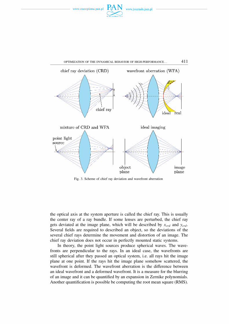
The imaging quality of an optical system can be determined by differentdescriptions of aberrations [5]. In the special case of investigating the motionof lenses, a promising method is to distinguish between chief ray deviation(CRD) acrd and wavefront aberration (WFA) aw f a, see Fig. 3. In the lowerleft figure, a mixture of the two aberrations of the upper figures can be seen.The figure without any disturbance serves as contrast to the aberration drafts.It shows an ideal imaging as well as the object plane and image plane. Thelight always directs from the object to the image.

In geometrical optics, it is common to use point light sources which arethe starting point of a ray bundle, the so-called fields. The ray that crosses


Fig. 3. Scheme of chief ray deviation and wavefront aberration

the optical axis at the system aperture is called the chief ray. This is usuallythe center ray of a ray bundle. If some lenses are perturbed, the chief raygets deviated at the image plane, which will be described by xcrd and ycrd .Several fields are required to described an object, so the deviations of theseveral chief rays determine the movement and distortion of an image. Thechief ray deviation does not occur in perfectly mounted static systems.

In theory, the point light sources produce spherical waves. The wave-fronts are perpendicular to the rays. In an ideal case, the wavefronts arestill spherical after they passed an optical system, i.e. all rays hit the imageplane at one point. If the rays hit the image plane somehow scattered, thewavefront is deformed. The wavefront aberration is the difference betweenan ideal wavefront and a deformed wavefront. It is a measure for the blurringof an image and it can be quantified by an expansion in Zernike polynomials.Another quantification is possible be computing the root mean square (RMS).


2.3. Zernike polynomials

Zernike polynomials Z j are orthogonal polynomials with a unit circlebase, see [5,6]. They consist of a radial-dependent part

Rmn =

(n−m)/2∑

k=0

(−1)k(n − k)!k! ((n + m)/2 − k)! ((n − m)/2 − k)!

rn−2k (4)

with the normalized radius r and an angular-dependent part with the angle φ.The indices m and n are positive integers with n ≥ m. There exist differentnotations for the polynomials. Here, the standard notation introduced in [7] isused due to its advantages in computer programming. The Zernike standardpolynomials Z j read

Z j(r, φ) =√

2(n + 1) Rmn(r) cos(mφ), if m , 0 and j even,

Z j(r, φ) =√

2(n + 1) Rmn(r) sin(mφ), if m , 0 and j odd,

Z j(r) =√

n + 1 Rmn(r), if m = 0.

(5)

The expansion of aw f a in k Zernike polynomials Z j means describingthe wavefront aberration by k Zernike coefficients c j,

aw f a = [c1, c2, . . . ck]T . (6)

This corresponds to a subdivision into characteristic aberrations which are,e.g., defocus (Z4), spherical aberration (Z11), coma, etc. The coefficients c jare used to describe the wavefront aberration and, therefore, the blurring ofthe projected image. The wavefront aberration is a circular area ζ definedby discrete points and it is scaled to the unit circle. Generally, the wavefrontaberration evaluated by Zernike polynomials reads

ζ =∑

c jZ j. (7)

In index notation, each discrete point ζi(ri, θi) of the wavefront aberration isdefined by Z j,i(ri, θi),

ζi = [Z1,i, Z2,i, . . . Zk,i] · aw f a (8)

where the coefficients in aw f a are unknown. The equation system derivedfor all discrete points is usually overdetermined and has to be solved by aleast-squares algorithm.


2.4. Dynamical-optical sensitivities

In the case of small movements, the aberrations acrd and aw f a are pro-portional to the lens movements y of Eq. (3). This can be expressed by thedynamical-optical sensitivities S,

a =

acrd

aw f a

= S · y (9)

with the sensitivities S = [S1, S2, ... Sk] for k lenses and, considering a singlefield, for one lens i

Si =

xcrd,x xcrd,y xcrd,z xcrd,θx xcrd,θy

ycrd,x ycrd,y ycrd,z ycrd,θx ycrd,θy

c1,x c1,y c1,z c1,θx c1,θy...

......

......

ck,x ck,y ck,z ck,θxck,θy

. (10)

Each column represents the aberrations of a unity movement in one degreeof freedom. Then, inserting Eq. (3) in Eq. (9) leads to

a = S · C︸︷︷︸Cs

· q. (11)

The sensitivities in S are strictly related to the design of the optical system.When investigating a certain optical design, S has to be calculated onlyonce. For each column in S, one raytracing simulation is required. Once S isknown, using Eq. (11) is advantageous for simulations in the time domain.The other possibility would be calculating the aberrations at each time stepwhich is, in general, less efficient.

2.5. A formalism including modal transformation

The previously discussed sensitivities will now be expanded to a methodwhich is essential for the optimization process. This method allows for a di-rect evaluation of the dynamical design quality of an optomechanical system.Therefore, the main idea of this method will be used in Section 3.1. to definethe objective function of the optimization.

The characteristics of a dynamical system described by Eq. (2) can beinvestigated by means of the eigenvalue problem

(K − ω2

jM)· φ j = 0 (12)


with the j-th eigenfrequency ω j and the associated mode shape φ j. When avibrating system is freezed at an arbitrary point in time t∗, the state of thesystem is a superposition of the mode shapes,

q(t∗) =

n∑

j=1

d j(t∗)φ j (13)

with d j being the amplitudes of the corresponding mode shapes and n beingthe number of degrees of freedom. The n mode shapes can be summarizedin

Φ = [ φ1, φ2, . . . φn ]. (14)

For the following calculations, the mode shapes Φ will be used to scale themass matrix

ΦT ·M ·Φ = I (15)

where I is the identity matrix. Using the substitution q = Φ · q with themodal coordinates q and premultiplying Eqs. (2) and (3) by ΦT leads to themodally transformed equations of motion,

ΦT ·M ·Φ · ¨q + ΦT · D ·Φ · ˙q + ΦT · K ·Φ · q = ΦT · B · u (16)y = C ·Φ · q. (17)

The modal coordinates q are equal to the amplitudes d j in Eq. (13). Usingthe scaling of Eq. (15), Eq. (16) becomes

¨q + diag(2ωiξi) · ˙q + diag(ω2i ) · q = B · u. (18)

Inserting Eq. (17) in Eq. (9) yields

a = S · C ·Φ︸︷︷︸Cs

· q. (19)

The matrix Cs indicates the aberrations of a mode shape. This matrix caneither be calculated like in Eq. (19), or can be computed by applying the lensmovements of the mode shapes to the optical system and doing a raytracingsimulation. Using Eq. (19), we now can compute the optical aberrations afrom the modally described lens movements q.


3. Optimization of the mode shapes

Usually, the mechanical design for an optical system is customized withrespect to the optical design. So it is the idea of this method to improvean existing mechanical design without touching the optical design. Here,improving the design means systematically adjusting mode shapes whichproduce small aberrations. The improved dynamical behavior can be found bymeans of numerical optimization methods where the masses and stiffnessesare adjusted.

3.1. The performance function

In dynamical systems, knowing the input/output behavior is essential.Here, the input is an excitation and the outputs are the aberrations a. Thebehavior is described by a dynamical-optical transfer function H(iω) derivedfrom the modally transformed system in Eqns. (18) and (19)

‖H(iω)‖ =

n∑

j=1

‖[Cs]∗ j[B] j∗‖−ω2 + ω2

j + 2iωω jξ j. (20)

The product [Cs]∗ j[B] j∗ is the dyadic product of the j-th column of Cs andthe j-th row of B. Following from Eqn. (20), the substitution

woptical, j =‖[Cs]∗ j[B] j∗‖

ω j(21)

determines the influence of an unitary sinusoidal excitation on the aberra-tion of a mode shape. Using woptical, j as weighting factor, the optimizationproblem

min f (p) with f (p) =

k∑

j=1

|Cs · woptical, j φ j | (22)

subject to pmin ≤ p ≤ pmax

is specified by the sum of the weighted aberrations of k selected modeshapes.

Before or during the optimization, mode shapes have to be selected. Forthis, the user has two possibilities. On the one hand, he can in advance selectmode shapes by their number. On the other hand, he can chose a frequencyrange. All mode shapes corresponding to an eigenfrequency within this rangewill then be selected during the evaluation of the performance function.


It is additionally possible to ’weight’ the mode shapes by their eigen-frequencies. For this, the function wexcitation(ω) has to be defined, whichrepresents the frequency spectrum of the excitation of the simulation model.This frequency spectrum is known or should at least be guessed from expe-rience. The quality of the optimization results increases with the accuracy ofthe frequency spectrum estimation. Multiplying wexcitation(ω j) with woptical, jleads to a new weighting factor w j which replaces woptical, j in the performancefunction,

f (p) =

k∑

j=1

|Cs · w j φ j |. (23)

3.2. Software implementation of the optimization

The software implementation of the computation of the performancefunction contains the generation of the mass and stiffness matrix, solving theeigenvalue problem, scaling the eigenvectors and computing the performancefunction f (p) using Eqn. (23). A basic scheme is shown in Fig. 4.

Fig. 4. The optimization process

A disadvantage of the method shown is the requirement of a solution ofthe eigenvalue problem in each iteration step. Increasing the performance ispossible by calculating only a fixed number of smallest eigenvalues.

Sometimes in optimizing dynamical systems, the transfer function for afrequency range is summed up in each iteration step in order to calculate


the performance function. However, if damping is neglected, this leads toinaccuracies due to the peaks at the eigenfrequencies. Furthermore, a matrixinversion is required for computing the transfer function.

The performance function has usually many local minima, thus a stochas-tic optimization algorithm is required to ensure good solutions. Here, a Par-ticle Swarm Optimization (PSO) algorithm named ALSPO [8] is used whichis written in Matlab and treats constraints using an Augmented LagrangianOptimization technique. For general information about PSO see [9,10].

The results are compared to a deterministic algorithm for which theSequential Quadratic Programming (SQP) method is chosen. In general, theNLPQL algorithm [11] in the Matlab implementation fmincon() yields goodresults and, therefore, will be applied here.

Optimization algorithms usually require a scaling of the design parame-ters,

pi = ( pmax − pmin)pi − pmin,i

pmax,i − pmin,i− pmin with pmin ≤ p ≤ pmax. (24)

In the following computations, pmin = −10 and pmax = 10 are used.

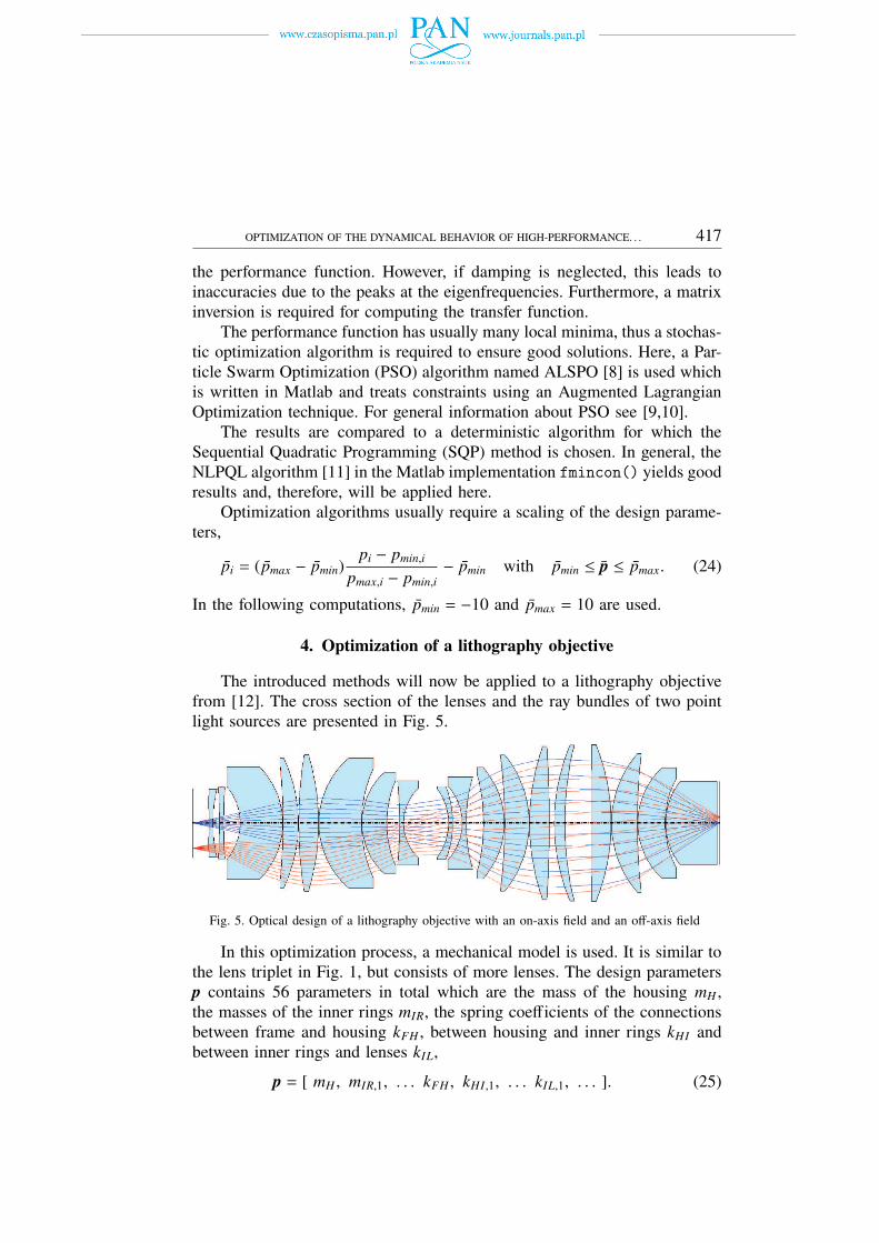
4. Optimization of a lithography objective

The introduced methods will now be applied to a lithography objectivefrom [12]. The cross section of the lenses and the ray bundles of two pointlight sources are presented in Fig. 5.

Fig. 5. Optical design of a lithography objective with an on-axis field and an off-axis field

In this optimization process, a mechanical model is used. It is similar tothe lens triplet in Fig. 1, but consists of more lenses. The design parametersp contains 56 parameters in total which are the mass of the housing mH ,the masses of the inner rings mIR, the spring coefficients of the connectionsbetween frame and housing kFH , between housing and inner rings kHI andbetween inner rings and lenses kIL,

p = [ mH , mIR,1, . . . kFH , kHI ,1, . . . kIL,1, . . . ]. (25)


The optimization process comprises the optimization of transversal mo-tion. The motion is only represented by movements in y-direction and thex-direction is left out since the lens system is assumed to be rotationallysymmetric about the z-axis. Unfortunately, either chief ray deviation or wave-front aberration can be minimized. Minimizing both simultaneously wouldrequire a multi-objective optimization, so here, only the chief ray deviationis concerned in the performance function.

To give an overview about several sets of design parameters, four differentresults/ choices will be presented. Regarding industrial applications, it is typ-ical to improve existing designs. So the first design is the initial guess pinitialwhich is meant to represent an existing but not yet mathematically optimizedguess. Then, there are two optimized designs, an SQP-optimized popt,sqp forthe deterministic solution and the PSO-optimized popt,pso. To compare themall to a poor design, pmaxerror with a maximum aberration is calculated bymaximizing the chief ray deviation with the ALPSO algorithm. This givesan idea about how a bad design might look like.

4.1. Excitation model for time simulations

To validate the optimization results, simulations in the time domain withsubsequent image simulations are performed. For the time simulations, anexcitation is required, which is applied at the housing of the objective, seeFig. 6. Once the lens movements are calculated, the aberrations can be com-puted and can be visualized by means of geometric image simulations.

As stated in Section 3.2, practically meaningful optimization results willbe obtained if an additional weighting of the mode shapes matches the fre-quency spectrum of the excitation. In the following example, the force exci-tation in Fig. 6 will be used for validations in the time domain. This forcecorresponds to a shock of a soft hammer. Thus, the system is able to performfree vibrations after a short excitation. The curve of the Fourier transformserves as the additional weighting function wexcitation within the performancefunction to weight the aberrations of the selected mode shapes.

4.2. Optimization results

The transfer behaviors in Fig. 7 show the results of optimizing thetransversal motion. The four models are subjected to an input at the hous-ing, and the chief ray deviation of the on-axis field serves as criterionof the optimization. The curves of the optimized models are significant-ly lower than those of the other two designs. Accordingly, the aberrationswill be lower. It can be stated that the optimizations succeeded and themethod works in the frequency domain. The values of the performance func-


Fig. 6. Mechanical model with the hammer shock excitation (left), time history of the shock of a

soft hammer and its Fourier transform (right)

tions are f (pinitial) = 11.852, f (pmaxerror) = 25.923, f (popt,sqp) = 0.393 andf (popt,pso) = 0.065.

Fig. 7. Transfer functions of the four dynamical-optical models

For the validation in the time domain, Fig. 8 represents the results forthe two optimized designs. Here, the difference between popt,sqp and popt,psois even more obvious than in Fig. 7. Additionally, the RMS of the wavefront


aberration is given although only the chief ray deviation has been optimized.At the beginning of the simulation, there is a peak in all curves which resultsfrom the hammer shock. Furthermore, popt,sqp exhibits beats in both the chiefray deviation and the wavefront aberration in phase. The beats do not occurfor the PSO-optimized parameters which makes them better than the SQP-optimized parameters.

Fig. 8. Chief ray deviation and wavefront aberration after a hammer shock on the housing of the

two optimized models

A comparison in the time domain of all four models is summarized inFig. 9. With the time range of 0 to 10 seconds, as in Fig. 8, the RMS valuesof the aberration curves are computed. For both aberration types the ratiosof the reduction are approximately equal and they correspond to the ratios ofthe performance function results. However, the wavefront aberration is notincluded in the performance function and thus, its minimization is a sideeffect of the optimization. As the diagrams show, the PSO method yields thelowest aberrations in both cases.

4.3. Geometric image simulations

A geometric image simulation comprises a raytracing simulation with atest object where millions of rays start with random direction from randompoint light sources. The image screen is subdivided into pixels. At eachpixel, the hitting rays are counted which yields an intensity distribution ofa projected image. Integrating the intensity distribution over a time rangeyields a map for the energy distribution of an exposure.

The exposure of the letter ’F’ is demonstrated in Fig. 10. In this example,the same parameter sets and excitation as in the previous section are used. Thetime range of the exposure is 2.0 to 2.3 seconds. Expectedly, the images of


Fig. 9. RMS of the chief ray deviation curve and the wavefront aberration curve after a hammer

shock in y-direction

the non-optimized models are more blurred due to large vertical movements.These movements are much smaller for the images of the optimized models.Thus, the image quality is improved significantly. The blurring at the verticaledges is mainly due to the system-inherent aberrations.

Fig. 10. Image simulations over a time range for pointing out the effect of the hammer shock on a

projected image

5. Conclusions and Outlook

For optomechanical systems which can be modeled by rigid bodies theoptimization method in this paper can improve an existing design. The op-timization works most notably if it is applied to the expected frequencyspectrum of possible excitations.

Based on these methods, some expansions are possible to gain even betterresults. For example, including an adaptation of the optical design within theperformance function. This has to be implemented by an additional opti-


cal optimization regarding the dimensions of the lenses. Also, the influenceof lens deformations has to be taken into account. This is due to possiblechanges in the stiffness of the supports of the lenses which influences thedeformation behavior.

Acknowledgements

The authors would like to thank the German Research Foundation (DFG)for financial support of the project within the Cluster of Excellence in Sim-ulation Technology (EXC 310/1, SimTech) at the University of Stuttgart.Special thanks go to useful discussions and advice from the Institute of Ap-plied Optics (ITO), Holger Gilbergs, Karsten Frenner and Wolfgang Osten.All this support is highly appreciated.

Manuscript received by Editorial Board, September 23, 2011;final version, November 11, 2011.

REFERENCES

[1] Mack C.: Fundamental Principles of Optical Lithography. Chichester: John Wiley and Sons,2007.

[2] Schriever M., Wegmann U., Hembacher S., Geuppert B., Huber J., Kerwien N., TotzeckM., Hauf M.: Optical Apparatus and Method for Modifying the Image Behavior of suchApparatus. Patent US 2009/0174876, 2009.

[3] Shibazaki Y.: Optical Element Holding Apparatus. Patent US 2007/0121224, 2007.[4] Schiehlen W., Eberhard P.: Technische Dynamik – Modelle fur Regelung und Simulation (in

German). Wiesbaden: Teubner, 2004.[5] Born M., Wolf E.: Principles of Optics. Cambridge: University Press, 1999.[6] Zernike F.: Beugungstheorie des Schneidenverfahrens und seiner verbesserten Form, der

Phasenkontrastmethode (in German). Physica 1, pp. 689-704, 1934.[7] Noll R.: Zernike Polynomials and Atmospheric Turbulence. Journal of the Optical Society in

America, Vol. 66, No. 3, pp. 207-211, 1976.[8] Sedlaczek K., Eberhard P.: Using Augmented Lagrangian Particle Swarm Optimization for

Unconstrained Problems in Engineering. Structural and Multidiscipinary Optimization, Vol.32, No. 4, pp. 277-286, 2006.

[9] Sedlaczek K., Eberhard P.: Augmented Lagrangian Particle Swarm Optimization in Mecha-nism Design. Journal of System Design and Dynamics, Vol. 1, pp. 410-421, 2007.

[10] Kennedy J., Eberhart R.: Swarm Intelligence. San Diego: Academic Press, 2001.[11] Schittkowski K.: NLPQL: A Fortran Subroutine Solving Constrained Nonlinear Programming

Problems. Annals of Operations Research, Vol. 5, pp. 485-500, 1985.[12] Ulrich W., Rostalski H.J.: Projection Objective for Immersion Lithography. Patent US

2010/0323299, 2010.


Optymalizacja właściwości dynamicznych systemów obiektywów o wysokiejdokładności w celu redukcji aberracji dynamicznych

S t r e s z c z e n i e

W systemach obiektywów wysokiej klasy nawet małe zakłócenia mogą spowodować nieostrośćprojekcji obrazu. Ogromny problem dla tych niezwykle precyzyjnych systemów optyczno-mechani-cznych stanowią na przykład niewielkie pobudzenia o charakterze stochastycznym. Jest do pomyśle-nia szereg środków, by uniknąć związanych z tym problemów, a przynajmniej by je ograniczyć.Jedną z takich możliwości jest modyfikacja właściwości dynamicznych. W metodzie tej, w celuzmniejszenia aberracji powodowanych przez pobudzenia dynamiczne, stosuje się redystrybucję masi sztywności systemu.

Wymagany w tym przypadku jest multidyscyplinarny proces optymalizacyjny, dla potrzebktórego w artykule wprowadza się podstawy połączonych dynamicznych i optycznych metod sty-mulacji. Optymalizacja jest oparta na metodzie zapewniającej efektywne połączenie tych dwu typówstymulacji. W końcowym przykładzie przedstawiono optymalizację dynamiki ciała sztywnegoreprezentującego obiektyw litograficzny pod kątem jego właściwości dynamiczno-optycznych.

optimization of the dynamical behavior of high …

Documents