optimization with the nature-inspired intelligent water drops

16

Optimization with the Nature-Inspired Intelligent Water Drops Algorithm

Hamed Shah-Hosseini Faculty of Electrical and Computer Engineering, Shahid Beheshti University, G.C.

Tehran, Iran

1. Introduction

Scientists are beginning to realize more and more that nature is a great source for inspiration in order to develop intelligent systems and algorithms. In the field of Computational Intelligence, especially Evolutionary Computation and Swarm-based systems, the degree of imitation from nature is surprisingly high and we are at the edge of developing and proposing new algorithms and/or systems, which partially or fully follow nature and the actions and reactions that happen in a specific natural system or species. Among the most recent nature-inspired swarm-based optimization algorithms is the Intelligent Water Drops (IWD) algorithm. IWD algorithms imitate some of the processes that happen in nature between the water drops of a river and the soil of the river bed. The IWD algorithm was first introduced in (Shah-Hosseini, 2007) in which the IWDs are used to solve the Travelling Salesman Problem (TSP). The IWD algorithm has also been successfully applied to the Multidimensional Knapsack Problem (MKP) (Shah-Hosseini, 2008a), n-queen puzzle (Shah-Hosseini, 2008b), and Robot Path Planning (Duan et al., 2008). Here, the IWD algorithm and its versions are specified for the TSP, the n-queen puzzle, the MKP, and for the first time, the AMT (Automatic Multilevel Thresholding). Some theoretical findings have also been reviewed for the IWD algorithm. Next section reviews briefly the related works. Section 3 examines natural water drops. Section 4 states about Intelligent Water Drops (IWDs). Section 5 specifies the Intelligent Water Drops (IWD) algorithm. Next section, reviews the convergence properties of the IWD algorithm. Section 7 includes experiments with the IWD and its versions for the four mentioned problems. Final section includes the concluding remarks.

2. Related works

One of the famous swarm-based optimization algorithms has been invented by simulating the behaviour of social ants in a colony. Ants living in a nest are able to survive and develop their generations and reproduce in a cooperative way. Moreover, they can find the shortest path from their nest to a food source or vice versa. They can build complex nests capable of holding hundreds of thousands of ants and lots of other activities that show a high-level of intelligence in a colony of ants. Other social insects generally show such complex and intelligent behaviours such as bees and termites. Ant colony optimization (ACO) algorithm O

pen

Acc

ess

Dat

abas

e w

ww

.inte

chw

eb.o

rg

Source: Evolutionary Computation, Book edited by: Wellington Pinheiro dos Santos, ISBN 978-953-307-008-7, pp. 572, October 2009, I-Tech, Vienna, Austria

www.intechopen.com

Evolutionary Computation

298

(Dorigo & et al., 1991) and Bee Colony Optimization (BCO) algorithm (Sato & Hagiwara, 1997) are among the swarm-based algorithms imitating social insects for optimization. Evolutionary Computation is another system, which has been inspired from observing natural selection and reproduction systems in nature. Genetic algorithms (GA) (Holland, 1975) are among the most famous algorithms in this regard. Evolution Strategy (Rechenberg, 1973; Schwefel, 1981), Evolutionary Programming (Fogel et al., 1966), and Genetic Programming (Koza, 1992) are other Evolutionary-based intelligent algorithms that are often used for optimization. Memetic Algorithms (MA) (Dawkins, 1989; Ong et al., 2006) are among the most recent area of research in the field of Evolutionary Computation. Here, a meme is the basic unit of culture that can be inherited. An individual is assumed to have both genes and memes. Therefore, not only the genes of individuals evolve, but also their memes undergo evolution. Artificial Immune Systems (AIS) are another example of swarm-based nature inspired algorithms, which follow the processes and actions that happen in the immune systems of vertebrates. Clonal Selection Algorithms (de Castro & Von Zuben, 2002), Negative Selection Algorithms (Forrest, et al., 1994), and Immune Network Algorithms (Timmis et al., 2000) are among the most common techniques in the field of AIS. Another swarm-based optimization algorithm is the Particle Swarm Optimization (PSO), which has been introduced by (Kennedy & Eberhart, 1995). PSO uses a swarm of particles, which each one has position and velocity vectors, and they move near together to find the optimal solution for a given problem. Infact, PSO imitates the processes that exist in the flocks of birds or a school of fish to find the optimal solution. Another swarm-based optimization algorithm is the Electromagnetism-like mechanism (EM) (Birbil & Fang, 2003). The EM algorithm uses an attraction-repulsion mechanism based on the Coulomb’s law to move some points towards the optimal positions.

3. Natural water drops

In nature, flowing water drops are observed mostly in rivers, which form huge moving swarms. The paths that a natural river follows have been created by a swarm of water drops. For a swarm of water drops, the river in which they flow is the part of the environment that has been dramatically changed by the swarm and will also be changed in the future. Moreover, the environment itself has substantial effects on the paths that the water drops follow. For example, against a swarm of water drops, those parts of the environment having hard soils resist more than the parts with soft soils. In fact, a natural river is the result of a competition between water drops in a swarm and the environment that resists the movement of water drops. Based on our observation in nature, most rivers have paths full of twists and turns. Up until now, it is believed that water drops in a river have no eyes so that by using those eyes, they can find their destination, which is often a lake or sea. If we put ourselves in place of a water drop flowing in a river, we would feel that some force pulls us toward itself, which is the earth’s gravity. This gravitational force pulls everything toward the center of the earth in a straight line. Therefore with no obstacles and barriers, the water drops should follow a straight path toward the destination, which is the shortest path from the source of water drops to the destination, which is ideally the earth’s center. This gravitational force creates acceleration such that water drops gain speed as they come near to the earth’s center. However, in reality, due to different kinds of obstacles and constraints in the way of this

www.intechopen.com


299

ideal path, the real path is so different from the ideal path such that lots of twists and turns in a river path are seen, and the destination is not the earth’s center but a lake, sea, or even a bigger river. It is often observed that the constructed path seems to be an optimal one in terms of the distance from the destination and the constraints of the environment. One feature of a water drop flowing in a river is its velocity. It is assumed that each water drop of a river can also carry an amount of soil. Therefore, the water drop is able to transfer an amount of soil from one place to another place in the front. This soil is usually transferred from fast parts of the path to the slow parts. As the fast parts get deeper by being removed from soil, they can hold more volume of water and thus may attract more water. The removed soils, which are carried in the water drops, are unloaded in slower beds of the river. Assume an imaginary natural water drop is going to flow from one point of a river to the next point in the front. Three obvious changes happen during this transition:

• Velocity of the water drop is increased.

• Soil of the water drop is increased.

• Between these two points, soil of the river’s bed is decreased. In fact, an amount of soil of the river’s bed is removed by the water drop and this removed soil is added to the soil of the water drop. Moreover, the speed of the water drop is increased during the transition. It was mentioned above that a water drop has also a velocity. This velocity plays an important role in removing soil from the beds of rivers. The following property is assumed for a flowing water drop:

• A high speed water drop gathers more soil than a slower water drop. Therefore, the water drop with bigger speed removes more soil from the river’s bed than another water drop with smaller speed. The soil removal is thus related to the velocities of water drops. It has been said earlier that when a water drop flows on a part of a river’s bed, it gains speed. But this increase in velocity depends on the amount of soil of that part. This property of a water drop is expressed below:

• The velocity of a water drop increases more on a path with low soil than a path with high soil.

The velocity of the water drop is changed such that on a path with little amount of soil, the velocity of the water drop is increased more than a path with a considerable amount of soil. Therefore, a path with little soil lets the flowing water drop gather more soil and gain more speed whereas the path with large soil resists more against the flowing water drop such that it lets the flowing water drop gather less soil and gain less speed. Another property of a natural water drop is that when it faces several paths in the front, it often chooses the easier path. Therefore, the following statement may be expressed:

• A water drop prefers a path with less soil than a path with more soil The water drop prefers an easier path to a harder path when it has to choose between several branches that exist in the path from the source to destination. The easiness or hardness of a path is denoted by the amount of soil on that path. A path with more soil is considered a hard path whereas a path with less soil is considered an easy path.

4. Intelligent Water Drops (IWDs)

In the previous section, some prominent properties of natural water drops were mentioned. Based on the aforementioned statements, an Intelligent Water Drop (IWD) has been

www.intechopen.com


300

suggested (Shah-Hosseini, 2007), which possesses a few remarkable properties of a natural water drop. This Intelligent Water Drop, IWD for short, has two important properties:

• The soil it carries, denoted by soil(IWD).

• The velocity that it posses, denoted by velocity(IWD). For each IWD, the values of both properties, soil(IWD) and velocity(IWD) may change as the IWD flows in its environment. From the engineering point of view, an environment represents a problem that is desired to be solved. A river of IWDs seeks an optimal path for the given problem. Each IWD is assumed to flow in its environment from a source to a desired destination. In

an environment, there are numerous paths from a given source to a desired destination. The

location of the destination may be unknown. If the location of the desired destination is

known, the solution to the problem is obtained by finding the best (often the shortest) path

from the source to the destination. However, there are cases in which the destination is

unknown. In such cases, the solution is obtained by finding the optimum destination in

terms of cost or any other desired measure for the given problem.

An IWD moves in discrete finite-length steps in its environment. From its current location i

to its next location j, the IWD velocity, velocity (IWD), is increased by an amount Δvelocity

(IWD), which is nonlinearly proportional to the inverse of the soil between the two locations

i an j, soil(i , j):

),(

1)(

jisoilIWDvelocity NL∝Δ (1)

Here, nonlinearly proportionality is denoted by ∝NL . One possible formula is given below in

which the velocity of the IWD denoted by )(tvel IWD is updated by the amount of soil

),( jisoil between the two locations i and j:

),( .

)(2 jisoilcb

atvel

vv

vIWD α+=Δ (2)

Here, the va ,

vb , vc , and α are user-selected positive parameters.

Moreover, the IWD’s soil, soil(IWD), is increased by removing some soil of the path joining

the two locations i an j. The amount of soil added to the IWD, Δsoil(IWD)= Δsoil(i,j), is

inversely (and nonlinearly) proportional to the time needed for the IWD to pass from its

current location to the next location denoted by time(i,j; IWD).

);,(

1),()(

IWDjitimejisoilIWDsoil NL∝Δ=Δ (3)

One suggestion for the above formula is given below in which );,( IWDveljitime is the time

taken for the IWD with velocity IWDvel to move from location i to j. The soil added to the

IWD is calculated by

( ) ;, .),(

2 IWDss

s

veljitimecb

ajisoil θ+=Δ (4)

www.intechopen.com


301

Where the parameters sa ,

sb , sc , and θ are user-selected and should be chosen as positive

numbers. The duration of time for the IWD is calculated by the simple laws of physics for linear

motion. Thus, the time taken for the IWD to move from location i to j is proportional to the

velocity of the IWD, velocity (IWD), and inversely proportional to the distance between the

two locations, d(i,j). More specifically:

)(

1);,(

IWDvelocityIWDjitime L∝ (5)

Where ∝L denotes linear proportionality. One such formula is given below, which calculates

the time taken for the IWD to travel from location i to j with velocity IWDvel :

( )IWD

IWD

vel

jiHUDveljitime

),(;, = (6)

Where a local heuristic function .) , (.HUD has been defined for a given problem to measure

the undesirability of an IWD to move from one location to the next. Some soil is removed from the visited path between locations i and j. The updated soil of the

path denoted by soil(i,j) is proportional to the amount of soil removed by the IWD flowing

on the path joining i to j, Δsoil(i,j)= Δsoil(IWD). Specifically:

),(),( jisoiljisoil L Δ∝ (7)

One such formula has been used for the IWD algorithm such that ),( jisoil is updated by

the amount of soil removed by the IWD from the path i to j.

),( . ),( . ),( jisoiljisoiljisoil no Δ−= ρρ (8)

Where oρ and

nρ are often positive numbers between zero and one. In the original IWD

algorithm for the TSP (Shah-Hosseini, 2007), no ρρ −=1 .

The soil of the IWD denoted by IWDsoil is added by the amount ),( jisoil as shown below:

),( jisoilsoilsoil IWDIWD Δ+= (9)

Another mechanism that exists in the behaviour of an IWD is that it prefers the paths with

low soils on its beds to the paths with higher soils on its beds. To implement this behaviour

of path choosing, a uniform random distribution is used among the soils of the available

paths such that the probability of the IWD to move from location i to j denoted by p(i,j;IWD)

is inversely proportional to the amount of soils on the available paths.

),();,( jisoilIWDjip L∝ (10)

The lower the soil of the path between locations i and j, the more chance this path has for

being selected by the IWD located on i. One such formula based on Eq. (10) has been used

in which the probability of choosing location j is given by:

www.intechopen.com


302

( )( )∑∉=)(

),(

),();,(

IWDvck

kisoilf

jisoilfIWDjip (11)

Where )),((

1)),((

jisoilgjisoilf

s += ε . The constant parameter sε is a small positive

number to prevent a possible division by zero in the function (.)f . The set )(IWDvc

denotes the nodes that the IWD should not visit to keep satisfied the constraints of the problem.

The function )),(( jisoilg is used to shift the ),( jisoil of the path joining nodes i and j

toward positive values and is computed by

⎪⎩⎪⎨⎧

−≥=

∉∉

elselisoiljisoil

lisoilif jisoil

jisoilg

IWDvcl

l

)),((min),(

0)),((min ),(

)),((

)(

vc(IWD) (12)

Where the function min(.) returns the minimum value of its arguments. The IWDs work together to find the optimal solution to a given problem. The problem is encoded in the environment of the IWDs, and the solution is represented by the path that the IWDs have converged to. In the next section, the IWD algorithm is explained.

5. The Intelligent Water Drops (IWD) algorithm

The IWD algorithm employs a number of IWDs to find the optimal solutions to a given

problem. The problem is represented by a graph ( )EN , with the node set N and edge set E.

This graph is the environment for the IWDs and the IWDs flow on the edges of the graph.

Each IWD begins constructing its solution gradually by traveling between the nodes of the

graph along the edges until the IWD finally completes its solution denoted by IWDT . Each

solution IWDT is represented by the edges that the IWD has visited. One iteration of the

IWD algorithm is finished when all IWDs complete their solutions. After each iteration, the

iteration-best solution IBT is found. The iteration-based solution

IBT is the best solution

based on a quality function among all solutions obtained by the IWDs in the current

iteration. IBT is used to update the total-best solution

TBT . The total-best solution TBT is

the best solution since the beginning of the IWD algorithm, which has been found in all

iterations.

For a given problem, an objective or quality function is needed to measure the fitness of

solutions. Consider the quality function of a problem to be denoted by (.) q . Then, the

quality of a solution IWDT found by the IWD is given by )( IWDTq . Therefore, the iteration-

best solution IBT is given by:

)(maxarg

IWD

IWDsallfor

IB TqT = (13)

Where arg(.) returns its argument.

It should be noted that at the end of each iteration of the algorithm, the total-best solution TBT is updated by the current iteration-best solution

IBT as follows:

www.intechopen.com


303

⎪⎩⎪⎨⎧ ≥=

otherwiseT

TqTqifTT

IB

IBTBTBTB

)( )( (14)

Moreover, at the end of each iteration of the IWD algorithm, the amount of soil on the edges

of the iteration-best solution IBT is reduced based on the goodness (quality) of the solution.

One such mechanism (Shah-Hosseini, 2007) is used to update the ),( jisoil of each edge

),( ji of the iteration-best solution IBT :

IBIWD

IB

IB

IWD TjisoilN

jisoiljisoil

∈∀−=

),( . 1)-(

1 .

),( . ),( s

ρρ

(15)

Where IWD

IBsoil represents the soil of the iteration-best IWD. The iteration-best IWD is the

IWD that has constructed the iteration-best solution IBT at the current iteration.

IBN is the

number of nodes in the solution IBT .

IWDρ is the global soil updating parameter, which

should be chosen from [ ]1,0 . sρ is often set as )1( IWDρ+ .

Then, the algorithm begins another iteration with new IWDs but with the same soils on the

paths of the graph and the whole process is repeated. The IWD algorithm stops when it

reaches the maximum number of iterations itermax or the total-best solution TBT achieves the

expected quality demanded for the given problem. The IWD algorithm has two kinds of parameters:

• Static parameters

• Dynamic parameters Static parameters are those parameters that remain constant during the lifetime of the IWD algorithm. That is why they are called “static”. Dynamic parameters are those parameters, which are dynamic and they are reinitialized after each iteration of the IWD algorithm. The IWD algorithm as expressed in (Shah-Hosseini, 2008b) is specified in the following ten steps: 1. Initialization of static parameters:

• The graph ( )EN , of the problem is given to the algorithm, which contains cN nodes.

• The quality of the total-best solution TBT is initially set to the worst

value: −∞=)( TBTq .

• The maximum number of iterations maxiter is specified by the user and the algorithm

stops when it reaches maxiter .

• The iteration count countiter , which counts the number of iterations, is set to zero.

• The number of water drops IWDN is set to a positive integer value. This number should

at least be equal to two. However, IWDN is usually set to the number of nodes

cN of the

graph.

• Velocity updating parameters are va ,

vb , and vc . Here, 1== vv ca and 01.0=vb

• Soil updating parameters are sa ,

sb , and sc . Here, 1== ss ca and 01.0=sb

• The local soil updating parameter isnρ . Here, 9.0=nρ except for the AMT, which is

9.0−=nρ .

• The global soil updating parameter isIWDρ . Here, 9.0=IWDρ .

www.intechopen.com


304

• The initial soil on each edge of the graph is denoted by the constant InitSoil such that

the soil of the edge between every two nodes i and j is set by InitSoiljisoil =),( .

Here, 10000=InitSoil

• The initial velocity of each IWD is set to InitVel . Here, 200=InitVel except for the

MKP, which is 4=InitVel .

• Initialization of dynamic parameters:

• Every IWD has a visited node list )(IWDVc, which is initially empty: { }=)(IWDVc

.

• Each IWD’s velocity is set to InitVel .

• All IWDs are set to have zero amount of soil. 2. Spread the IWDs randomly on the nodes of the graph as their first visited nodes. 3. Update the visited node list of each IWD to include the nodes just visited. 4. Repeat steps 5.1 to 5.4 for those IWDs with partial solutions. 5.

5.1. For the IWD residing in node i, choose the next node j, which doesn’t violate any

constraints of the problem and is not in the visited node list )(IWDvc of the IWD,

using the following probability )( jp IWD

i:

( )( )∑∉=)(

),(

),()(

IWDvck

IWD

ikisoilf

jisoilfjp (16)

such that

)),((

1)),((

jisoilgjisoilf

s += ε (17)

and

⎪⎩⎪⎨⎧ −

≥=∉

∉elselisoiljisoil

lisoilif jisoiljisoilg

IWDvcl

l

)),((min ),(

0)),((min ),()),((

)(

vc(IWD) (18)

Then, add the newly visited node j to the list )(IWDvc .

5.2. For each IWD moving from node i to node j, update its velocity )(tvel IWD by

),( .

)()1(2 jisoilcb

atveltvel

vv

vIWDIWD ++=+ (19)

where )1( +tvel IWD is the updated velocity of the IWD.

5.3. For the IWD moving on the path from node i to j, compute the soil ),( jisoilΔ that the

IWD loads from the path by

( ))1(;, .),(

2 ++=Δtveljitimecb

ajisoil

IWD

ss

s (20)

such that ( ))1(

)()1(;, +=+

tvel

jHUDtveljitime

IWD

IWD where the heuristic undesirability

)( jHUD is defined appropriately for the given problem.

www.intechopen.com


305

5.4. Update the soil ),( jisoil of the path from node i to j traversed by that IWD, and also

update the soil that the IWD carries IWDsoil by

),(

),( . ),( . )1(),(

jisoilsoilsoil

jisoiljisoiljisoil

IWDIWD

nn

Δ+=Δ−−= ρρ

(21)

6. Find the iteration-best solution IBT from all the solutions

IWDT found by the IWDs using

)(maxarg IWD

T

IB TqTIWD∀= (22)

where function (.)q gives the quality of the solution.

7. Update the soils on the paths that form the current iteration-best solution IBT by

IBIWD

IB

IB

IWD TjisoilN

jisoiljisoil

∈∀−+=

),( . 1)-(

1 .

),( . )(1 ),( IWD

ρρ

(23)

where IBN is the number of nodes in solution

IBT .

8. Update the total best solution TBT by the current iteration-best solution

IBT using

⎩⎨⎧ ≥=

otherwiseT

TqTqifTT

IB

IBTBTB

TB

)( )( (24)

9. Increment the iteration number by 1+= countcount IterIter . Then, go to step 2 if

maxIterItercount < .

10. The algorithm stops here with the total-best solution TBT .

The IWD algorithm may be compared to the ant-based optimization algorithms (Bonabeau et al., 1999), which is summarized below:

• Every ant in an Ant Colony Optimization (ACO) algorithm deposits pheromones on

each edge it visits. In contrast, an IWD changes the amount of soil on edges.

• In the ACO algorithm, an ant cannot remove pheromones from an edge whereas in the

IWD algorithm, an IWD can both remove and add soil to an edge.

• In the IWD algorithm, the changes made on the soil of an edge are not constant and

they are dependent on the velocity and soil of the IWDs visiting that edge. In contrast,

in the ACO algorithm, each ant deposits a constant amount of pheromone on the edge.

• Besides, the IWDs may gain different velocities throughout an iteration of the IWD

algorithm whereas in ACO algorithms the velocities of the ants are irrelevant.

6. Convergence properties of the IWD algorithm

Let the graph ( )EN , represents the graph of the given problem. This graph is assumed to

be a fully connected graph with cN nodes. Let

IWDN represents the number of IWDs in the

IWD algorithm. In the soil updating of the algorithm, two extreme cases are considered:

www.intechopen.com


306

Case one: Only those terms of the IWD algorithm, which increase soil to an edge (arc) of ( )EN , , are considered.

Case two: Only those terms of the IWD algorithm, which decrease soil to an edge (arc) of ( )EN , , are considered.

For each case, the worst-case is followed. For case one, the highest possible value of soil that

an edge can hold after m iterations, )( maxedgesoil , will be (Shah-Hosseini, 2008a):

( )0max )( )( ISedgesoil m

osρρ= (25)

Where the edge is denoted by maxedge .

0IS is the initial soil of an edge ),( ji , which is

denoted by InitSoil in the IWD algorithm. 0ρ is used in Eq. (8) and

sρ is used in Eq. (15).

For case two, the lowest possible value of soil for an edge is computed. That edge is denoted

by maxedge . Then, after m iterations, the soil of

maxedge is (Shah-Hosseini, 2008a):

( ) ⎟⎟⎠⎞

⎜⎜⎝⎛ ⎟⎟⎠

⎞⎜⎜⎝⎛−=

s

sIWDnIWD

b

aNmedgesoil )( min ρρ (26)

Where IWDN is the number of IWDs. Soil updating parameters

sa and sb are defined in Eq.

(20). IWDρ is the global soil updating parameter used in Eq. (23).

nρ is the local soil

updating parameter used in Eq. (21). Based on Eqs. (25) and (26), the following proposition is stated:

Proposition 6.1. The soil of any edge in the graph ( )EN , of a given problem after m

iterations of the IWD algorithm remains in the interval [ ])(),( maxmin edgesoiledgesoil .

The probability of finding any feasible solution by an IWD in iteration m is )1()(

−cN

lowestp

where the probability of any IWD, going from node i to node j, is always bigger than lowestp .

It has been shown (Shah-Hosseini, 2008a) that lowestp is always a positive value. Since there

are IWDN IWDs, then the probability );( msp of finding any feasible solution s by the

IWDs in iteration m is:

)1(

)();(−= cN

lowestIWD pNmsp (27)

The probability of finding any feasible solution s at the end of M iterations of the

algorithm is:

( ));(11);(1

mspMsPm

M −Π−= = (28)

Because 1);(0 ≤< msp , then by making M large enough, it is concluded that:

( ) 0);(1 lim1

=−Π=∞→ mspm

M

M

. Therefore, the following proposition is true:

Proposition 6.2. If );( MsP represents the probability of finding any feasible solution s

within M iterations of the IWD algorithm. As M gets larger, );( MsP approaches to one:

1);(lim =∞→ MsP

M (29)

www.intechopen.com


307

Knowing the fact that the optimal solution *s is a feasible solution of the problem, from

above proposition, the following proposition is concluded.

Proposition 6.3. The IWD algorithm finds the optimal solution *s of any given problem

with probability one if the number of iterations M is sufficiently large.

It is noticed that the required M to find the optimal solution *s should be decreased by careful tuning of parameters of the IWD algorithm for the given problem.

7. Experimental results

Every IWD in the IWD algorithm both searches and changes its environment. During this search, the IWD incrementally constructs a solution. The problem definition is presented to the IWD algorithm in the form of a graph and IWDs visit nodes of the graph by travelling on the edges of the graph. A swarm of IWDs flows in the graph often with the guidance of a local heuristic in the hope of finding optimal or near optimal solutions. In the following, the IWD algorithm is used for four different problems: the TSP, the n-queen puzzle, the MKP, and for the first time, the IWD algorithm is used for Automatic Multilevel Thresholding (AMT).

7.1 The Travelling Salesman Problem (TSP) In the TSP (travelling salesman problem), a map of cities is given to the salesman and he is required to visit every city only once one after the other to complete his tour and return to its first city. The goal in the TSP is to find the tour with the minimum total length among all such possible tours for the given map.

A TSP is represented by a graph ( )EN , where the node set N denotes the n cities of the

TSP and the edge set E denotes the edges between cities. Here, the graph of the TSP is

considered a complete graph. Thus, every city has a direct link to another city. It is also

assumed that the link between each two cities is undirected. So, in summary, the graph of

the TSP is a complete undirected graph. A solution of the TSP having the graph ( )EN , is an

ordered set of n distinct cities. For such a TSP with n cities, there are ( 1)!/ 2n − feasible

solutions in which the global optimum(s) is sought.

A TSP solution for an n-city problem may be represented by the tour ( )ncccT ,...,, 21= . The

salesman travels from city 1c to

2c , then from 2c to

3c , and he continues this way until it

gets to city nc . Then, he returns to the first city

1c , which leads to the tour length (.)TL ,

defined by:

( ) ( )∑= += n

i

iin ccdcccTL1

121 , ,...,, (30)

such that 11 ccn =+ , and (.,.)d is the distance function, which is often the Euclidean

distance. The goal is to find the optimum tour ( )**

2

*

1 ,...,,* ncccT = such that for every other

feasible tour T :

)( *)( : TTLTTLT ≤∀ (31)

In order to use the IWD algorithm for the TSP, the TSP problem as mentioned above is

viewed as a complete undirected graph ( )EN , . Each link of the edge set E has an amount

www.intechopen.com


308

of soil. An IWD visits nodes of the graph through the links. The IWD is able to change the

amount of the soils on the links. Moreover, cities of the TSP are denoted by nodes of the

graph, which hold the physical positions of cities. An IWD starts its tour from a random

node and it visits other nodes using the links of the graph until it returns to the first node.

The IWD changes the soil of each link that it flows on while completing its tour. For the TSP, the constraint that each IWD never visits a city twice in its tour must be kept

satisfied. Therefore, for the IWD, a visited city list )(IWDVcis employed. This list includes

the cities visited so far by the IWD. So, the next possible cities for an IWD are selected from

those cities that are not in the visited list )(IWDVc of the IWD.

One possible local heuristic for the TSP, denoted by ) , ( jiHUDTSP, has been suggested

(Shah-Hosseini, 2008a) as follows:

)()( ),( jijiHUDTSP cc −= (32)

where )(kc denotes the two dimensional positional vector for the city k . The function .

denotes the Euclidean norm. The local heuristic ) , ( jiHUDTSP measures the undesirability

of an IWD to move from city i to city j . For near cities i and j , the heuristic measure

) , ( jiHUD becomes small whereas for far cities i and j , the measure ) , ( jiHUD

becomes big. It is reminded that paths with high levels of undesirability are chosen fewer

times than paths with low levels of undesirability. In the IWD algorithm, the time taken for

the IWD to pass from city i to city j , is proportional to the heuristic ) , ( jiHUDTSP.

A modification to the IWD-TSP has been proposed in (Shah-Hosseini, 2008b), which finds

better tours and hopefully escape local optimums. After a few number of iterations, say IN ,

the soils of all paths ),( ji of the graph of the given TSP are reinitialized again with the

initial soil InitSoil except the paths of the total-best solution TBT , which are given less soil

than InitSoil . The soil reinitialization after each IN iterations is expressed in the following

equation:

⎩⎨⎧ ∈Γ=

otherwiseInitSoil

TjieveryforInitSoiljisoil

TB

II

),( ),(

α (33)

where Iα is a small positive number chosen here as 0.1.

IΓ denotes a random number,

which is drawn from a uniform distribution in the interval [ ]1 , 0 . As a result, IWDs prefer

to choose paths of TBT because less soil on its paths is deposited. Here, 15=IN .

We may refer to the IWD algorithm for the TSP as the “IWD-TSP” algorithm. Moreover, the

modified IWD algorithm for the TSP is called the “MIWD-TSP” algorithm.

The MIWD-TSP algorithm is tested with cities on a circle such that the cities are equally

placed on the perimeter of the circle (Shah-Hosseini, 2008b). The number of cities is chosen

from 10 to 100 cities incremented by 10. The results of this experiment are shown in Table 1

in which the average numbers of iterations to get to the global optimums are depicted. The

number of IWDs is kept at the constant value 50. As the number of cities increases, the

average number of iterations to find the global optimum almost monotonically increases.

www.intechopen.com


309

No. of cities on the circle

10 20 30 40 50 60 70 80 90 100

Ave. iterations 10.4 39.6 78.6 85.5 134.5 181.9 253.1 364.7 387.4 404.5

Table 1. The average number of iterations to find the global optimum for the TSP where cities are equally spaced on the perimeter of a circle. The results are the average numbers of iterations of ten runs of the MIWD-TSP algorithm.

The IWD-TSP algorithm (Shah-Hosseini, 2007) for the TSPs of Table 1 often gets trapped

into local optimums. As the number of cities of the TSP increases, the average numbers of

iterations to get to the global optimums become high. For the TSPs with high numbers of

cities, it is impractical to use the IWD-TSP for them, and the MIWD-TSP is recommended. In

Fig. 1, such a local optimum is shown for the TSP with 10 cities along the tour obtained by

the MIWD-TSP algorithm.

Fig. 1. The IWD-TSP converges to a good local optimum in the left image. However, it has a small self-crossing in its tour for the TSP with 10 cities. In contrast, by using the MIWD-TSP, the self-crossing is removed and it converges to the tour in the right image.

Four TSPs are taken from the TSPLIB95 (the TSP Library in the Internet) to test the

performance of the MIWD-TSP algorithm (Shah-Hosseini, 2008b). The lengths of average

and best tours in five runs of the MIWD-TSP algorithm are reported in Table 2. For

comparison, the lengths of best tours of some other nature-inspired algorithms are also

mentioned in Table 2. The table shows that the tours obtained by the MIWD-TSP algorithm

are satisfactorily close to the known optimums and are comparable to the other nature-

inspired algorithms.

Method MIWD-TSP

Problem Name

Optimum length MMAS BCO EA

Improved ACO Best Average

eil51 426 426 431.13 --- 428.87 428.98 432.62 eil76 538 --- --- 544.36 --- 549.96 558.23 st70 675 --- 678.62 677.10 677.10 677.10 684.08

kroA100 21282 21282 21441.5 21285.44 --- 21407.57 21904.03

Table 2. The comparison between the Modified IWD-TSP and four other nature-inspired algorithms MMAS (Stutzle & Hoos, 1996), BCO (Teodorovic et al., 2006), EA (Yan et al., 2005), Improved ACO (Song et al., 2006) for the four TSPs mentioned below. The MIWD-TSP iterations: 3000 for eil51, 4500 for eil76, and 6000 for st70 and kroA100.

www.intechopen.com


310

The convergence curve for the TSP “eil51” with the MIWD-TSP algorithm is shown in Fig. 2 in which the tour length of the total-best solution versus iterations is depicted. Here, the algorithm converges to the tour of length 428.98, which is shown in the figure.

Convergence Curve for eil51

0

100

200

300

400

500

600

700

1 9 17 25 33 41 49 57 65 73 81 89 97 105

Iterations/15

Tour Length

Fig. 2. The MIWD-TSP algorithm converges to the tour length 428.98 for eil51. The converged tour is shown on the right side.

7.2 The n-queen puzzle

The n-queen puzzle is the problem in which n chess queens must be placed on an n×n chessboard such that no two queens attack each other (Watkins, 2004). The n-queen puzzle is the generalization of the 8-queen puzzle with eight queens on an 8×8 chessboard. The 8-quuen puzzle was originally proposed by the chess player “Max Bezzel” in 1848. Many mathematicians such as “Gauss” and “Cantor” have worked on the 8-queen puzzle and its generalized n-queen puzzle. The first solutions were provided by “Franz Nauck” in 1850. He also generalized it to the n-queen puzzle on an n×n chessboard. The 8-queen puzzle has 92 distinct solutions. If the solutions that differ only by rotations and reflections of the board are counted as one, the 8-queen puzzle has 12 unique solutions. Except for n=6, as the n increases, the number of unique (or distinct) solutions increases. A solution to the 8-queen puzzle is depicted in Fig. 3.

Fig. 3. A solution to the 8-queen puzzle on the chessboard.

One strategy is to put all n queens instantly on the n×n chessboard, which leads to the hug

search space nn2

(wrongly written n64 in (Shah-Hosseini, 2008b)). For 8=n , the search

space contains 14488 108.2264 ×≅= . To reduce the size of the search space of the n-queen

www.intechopen.com


311

problem, the n queens are placed one by one on the chessboard such that the first queen is

placed on any row of the first column. Then, the second queen is placed on any row of the

second column except the row of the first queen. Following this strategy, the ith queen is

placed on any row of the ith column except those rows that previous queens have occupied.

This incremental strategy of putting queens on the chessboard reduces the search space to

!n where the symbol “!” denotes the factorial. In the incremental strategy, if every row of the chessboard is considered a city, then the n-queen problem may be considered as a TSP. The first row chosen by the first queen is considered the first city of the tour. The second row chosen by the second queen is called the second city of the tour. Continuing this way, the ith row chosen by the ith queen is considered the ith city of the tour. The constraint that no two queens are in the same row is viewed as no two cities of the TSP graph are visited by the salesman. In summary, for the n-queen problem, a complete undirected TSP graph is created. In the n-queen puzzle, any feasible solution is also an optimal solution. Any feasible solution for an n-queen puzzle is the solution in which no two queens attack each other and that is the optimal solution. For this problem, the path to reach the final feasible (optimal) solution(s) is not wanted and in fact only the final positions of queens on the chessboard are desired.

The local heuristic undesirability ) , ( jiHUDNQ, which has been proposed in (Shah-

Hosseini, 2008b) to solve the n-queen puzzle, is stated as follows:

2

)1(),(n

jirjiHUDNQ −−+= (34)

where ) , ( jiHUDNQ is the undesirability of an IWD to go from current row (city) i to the

next row (city) j . Symbol |.| denotes the absolute value. The variable r is a random

number chosen uniformly from the interval [ ]1 , 0 . The symbol n denotes the number of

cities (columns or rows) of the chessboard of size nn× . In the above equation, the heuristic

favours the distance between the rows of neighbouring columns to be near the length 2

n.

However, it has been observed that the IWD algorithm with the mentioned local heuristic in Eq. (34) is usually trapped in the local optima in which only two queens attack each other. Sometimes, coming out of such local optima takes considerable iterations of the algorithm. For this purpose, a local search algorithm called “N-Queen Local Search” or NQLS has been proposed in (Shah-Hosseini, 2008b). This local search algorithm is activated when the

current iteration-best solution IBT of the IWD algorithm contains only two queens attacking

each other. Specifically, the NQLS algorithm is activated when the quality of the iteration-

best solution IBT , )( IBTq , becomes -1. The quality of a solution T denoted by )(Tq is

measured by

∑ ∑−= +=

−= 1

1 1

),()(n

i

n

ij

ji ccattackTq (35)

www.intechopen.com


312

Where 1),( =ji ccattack if queensic and

jc attack each other. Otherwise; 0),( =ji ccattack .

It is reminded that the optimal solution *T has the highest quality value zero: 0*)( =Tq . In the following, the NQLS is expressed in four steps:

1. Get the iteration-best solution IBT with tour ( )IB

n

IBIB ccc ,...,, 21 and 1)( −=IBTq .

2. initialize IBTT =0.

2. For 1,...,2,1 −= nk do the following steps (steps 2.1 to 2.3):

2.1. Shift the cities in the tour one position to the right such that the last city becomes

the first city in the tour: )( 1−= kk TshiftTRight

.

2.2. If 0)( =kTq , then set kTT =0

and go to step 4.

2.3. End loop.

3. For 1,...,2,1 −= nk do the following steps (steps 3.1 to 3.3):

3.1. Increment each city’s number (row) by one such that the highest row becomes the

lowest row in the chessboard: nkTT kk mod)( 1 += − , where mod is the modulus

function. Moreover, the increment inside the parenthesis is applied to each city of the

tour 1−kT .

3.2. If 0)( =kTq , then set kTT =0

and go to step 4. 3.3. End loop.

4. If 0)( 0 =Tq , then the total-best iteration solution TBT has been obtained and is

updated by 0TT TB = ; otherwise, no updating is implemented by this algorithm.

For simplicity, the IWD algorithm for the n-queen problem using the local search NQLS is called “IWD-NQ” algorithm. The IWD-NQ algorithm is tested with ten different n-queens puzzle (Shah-Hosseini, 2008b) where n is increased from 10 to 100 with step ten. The average number of iterations needed to find the optimal solution for ten runs of each n-queen puzzle is depicted in Fig. 4. It is reminded that 50 IWDs are used in the experiments. It is seen that the number of iterations to find the optimal solution(s) does not necessarily depend on the number of queens. For example, the average number of iterations for the 90-queen problem is bigger than the 100-queen problem.

10 30 50 70 90

0

500

1000

1500

2000

2500

3000

Itera

tions

no. queens

iterations versus queens

ave. iterations 759 261 348 210 190 602 510 547 2951 1294

10 20 30 40 50 60 70 80 90 100

Fig. 4. The average number of iterations to find the global optimums versus the number of queens for the n-queen puzzle. The results are the average iterations of ten runs of the IWD-NQ algorithm. The number of queens changes from 10 to 100.

www.intechopen.com


313

7.3 The multidimensional knapsack problem

The knapsack problem or KP is to select a subset of items i of the set I, each item i with the

profit ib and resource (capacity) requirement

ir such that they all fit in a knapsack of

limited capacity and the sum of profits of the selected items is maximized.

The multidimensional knapsack problem, MKP, is a generalization of the KP. In the MKP,

there exists multiple knapsacks and thus there are multiple resource constraints. The

inclusion of an item i in the m knapsacks is denoted by setting the variable iy to one,

otherwise iy is set to zero. Let the variable

ijr represents the resource requirement of an

item i with respect to the resource constraint (knapsack) j having the capacity ja . In other

words, ijr represents the amount of capacity that item i requires from knapsack j . The

MKP with m constraints (knapsacks) and n items wants to maximize the total profit of

including a subset of the n items in the knapsacks without surpassing the capacities of the

knapsacks. For the MKP, in more specific terms:

∑=n

i

iiby1

max (36)

subject to the following constraints:

mjforayrn

i

jiij ,...,2,1 1

=≤∑= (37)

where { } 1,0 ∈iy for ni ,...,2,1 = . Here, the profits ib and the resources requirements

ijr

are non-negative values. The MKP is an NP-hard combinatorial optimization problem with applications such as cutting stock problems, processor allocation in distributed systems, cargo loading, capital budgeting, and economics. Two general approaches maybe used for solving the MKP: the exact algorithms and the approximate algorithms. The exact algorithms are useful for solving small to moderate-size instances of the MKP such as those based on dynamic programming and those based on the branch-and-bound approach. For a more detail review on the MKP, Freville (2004) is suggested. The approximate algorithms may use nature-inspired approaches to approximately solve difficult optimization problems. Nature-inspired algorithms include algorithms such as Simulated Annealing (Kirkpatrick et al., 1983), Evolutionary Algorithms like Genetic Algorithms, Evolution Strategies, Evolutionary Programming, Ant Colony Optimization, Particle Swarm Optimization, Electromagnetism-like optimization, and Intelligent Water Drops (IWDs).

For the MKP, the local heuristic undesirability, denoted by )( jHUDMKP, is computed by:

∑== m

k

jkj

MKP rmb

jHUD1

1)( (38)

Where jb denotes the profit of item j and

jkr is the resource requirement for item j from

knapsack k . The above equation shows that )( jHUDMKP decreases if the profit

jb is high

www.intechopen.com


314

whereas )( jHUDMKP increases if the resource requirements of item j are high. As a

result, the items with less resource requirements and higher profits are more desirable.

)( jHUDMKP represents how undesirable is the action of selecting item j as the next item

to be included in the knapsacks. We may refer to the IWD algorithm used for the MKP as the IWD-MKP algorithm.

Quality of the IWD-MKP’s solution

no. of iterations of the IWD-MKP Problem

Name

Constraints

× Variables

Quality of Optimum solution Best Average Best Average

WEING1 2 × 28 141278 141278 141278 59 1243.8

WEING2 2 × 28 130883 130883 130883 154 618.4

WEING3 2 × 28 95677 95677 95677 314 609.8

WEING4 2 × 28 119337 119337 119337 4 48.5

WEING5 2 × 28 98796 98796 98796 118 698.5

WEING6 2 × 28 130623 130623 130623 71 970.3

WEING7 2 × 105 1095445 1094736 1094223 100 100

WEING8 2 × 105 624319 620872 617897.9 200 200

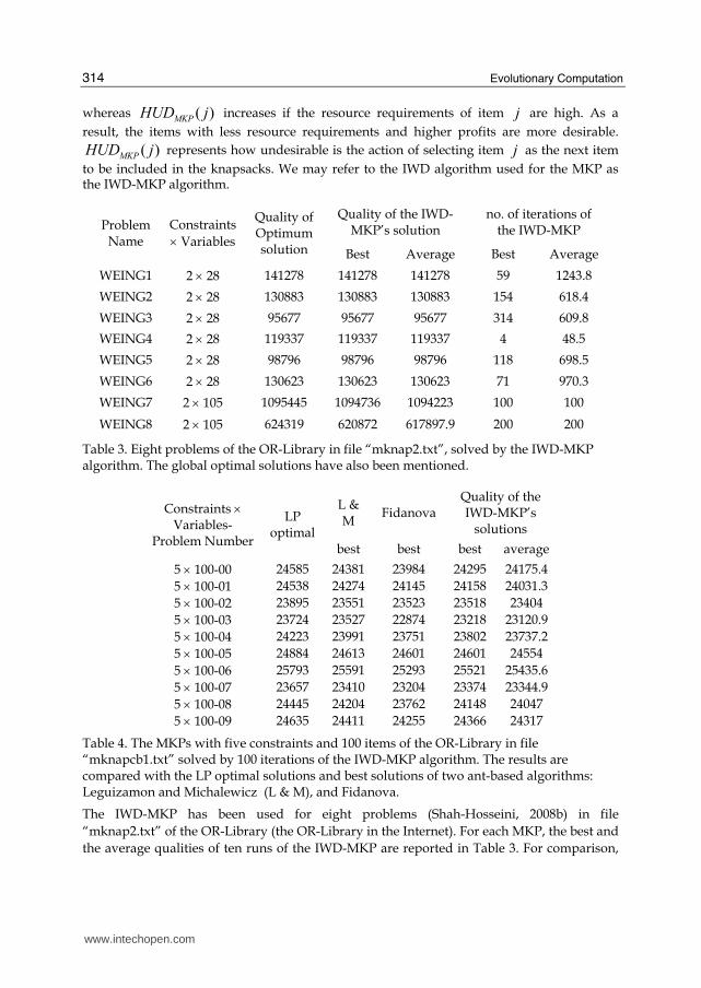
Table 3. Eight problems of the OR-Library in file “mknap2.txt”, solved by the IWD-MKP algorithm. The global optimal solutions have also been mentioned.

L & M

FidanovaQuality of the IWD-MKP’s

solutions

Constraints × Variables-

Problem Number

LP optimal

best best best average

5 × 100-00 24585 24381 23984 24295 24175.4

5 × 100-01 24538 24274 24145 24158 24031.3

5 × 100-02 23895 23551 23523 23518 23404

5 × 100-03 23724 23527 22874 23218 23120.9

5 × 100-04 24223 23991 23751 23802 23737.2

5 × 100-05 24884 24613 24601 24601 24554

5 × 100-06 25793 25591 25293 25521 25435.6

5 × 100-07 23657 23410 23204 23374 23344.9

5 × 100-08 24445 24204 23762 24148 24047

5 × 100-09 24635 24411 24255 24366 24317

Table 4. The MKPs with five constraints and 100 items of the OR-Library in file “mknapcb1.txt” solved by 100 iterations of the IWD-MKP algorithm. The results are compared with the LP optimal solutions and best solutions of two ant-based algorithms: Leguizamon and Michalewicz (L & M), and Fidanova.

The IWD-MKP has been used for eight problems (Shah-Hosseini, 2008b) in file

“mknap2.txt” of the OR-Library (the OR-Library in the Internet). For each MKP, the best and

the average qualities of ten runs of the IWD-MKP are reported in Table 3. For comparison,

www.intechopen.com


315

the qualities of optimal solutions are also mentioned in the table. The IWD-MKP algorithm

finds the global optimums for the first six MKPs with two constraints and 28 items.

However, the qualities of solutions of the problems “WEING7” and “WEING8” with two

constraints and 105 items obtained by the IWD-MKP are very close to the qualities of

optimal solutions. It is reminded that 50 IWDs are used in the mentioned experiments.

The first ten MKP problems in file “mknapcb1” of the OR-Library are solved by the IWD-

MKP and the results of ten runs of the algorithm are shown in Table 4. For comparison, the

results of the two Ant Colony Optimization-based algorithms of Leguizamon and

Michalewicz (for short, L & M) (Leguizamon and Michalewicz, 1999) and Fidanova

(Fidanova, 2002) are mentioned. Moreover, the results obtained by the LP relaxation method

that exist in the file “mkcbres.txt” of the OR-Library are also included. The solutions of the

IWD-MKP are often better than the solutions of those obtained by Fidanova.

7.4 Automatic multilevel thresholding

Image segmentation is often one of the main tasks in any Computer Vision application.

Image segmentation is a process in which the whole image is segmented into several regions

based on similarities and differences that exist between the pixels of the input image. Each

region should contain an object of the image at hand. Therefore, by doing segmentation, the

image is divided into several sub-images such that each sub-image represents an object of

the scene.

There are several approaches to perform image segmentation (Sezgin & Sankur, 2004). One

of the widely used techniques for image segmentation is multilevel thresholding. In doing

multilevel thresholding for image segmentation, it is assumed that each object has a distinct

continuous area of the image histogram. Therefore, by separating the histogram

appropriately, the objects of the image are segmented correctly.

Multilevel thresholding uses a number of thresholds { }Mttt ..., , , 21 in the histogram of the

image ),( yxf to separate the pixels of the objects in the image. By using the obtained

thresholds, the original image is multithresholded and the segmented image ( )),( yxfT is

created. Specifically:

( )⎪⎪⎩⎪⎪⎨⎧

≥<≤<

=MM tyxfifg

tyxftifg

tyxfifg

yxfT

),(

............. ....

),(

),(

),(211

10

(39)

Such that ig is the grey-level assigned to all pixels of the region i , which eventually

represents object i . As it is seen in the above equation, the 1+M regions are determined

by the M thresholds { }Mttt ..., , , 21. The value of

ig may be chosen to be the mean value of

gray-levels of the region’s pixels. However, in this paper we use the maximum range of

www.intechopen.com


316

gray-levels, 255, to distribute the gray-levels of regions equally. Specifically, ⎥⎦⎤⎢⎣

⎡=M

igi

255 .

such that the function [ ] . returns the integer value of its argument.

To multithreshold an image, the number of thresholds should be given in advance to a multilevel thresholding algorithm. However, a few algorithms have been designed to automatically determine the suitable number of thresholds based on the application at hand such as the Growing Time-Adaptive Self-Organizing Map (Shah-Hosseini & Safabakhsh, 2002). Such algorithms are called automatic multilevel thresholding. In automatic multilevel thresholding, the problem becomes harder because the search space increase hugely as the number of thresholds increases. For example, if the brightness of each image’s pixel be

selected from G different gray levels and the image is thresholded by M thresholds, then

the search space will be of size)!(

!

MG

G

− . For 256=G and 30=M , the search space is

approximately of size 71103× . It is reminded that in this paper, it is assumed that

256=G .

The AMT (Automatic Multilevel Thresholding) problem is converted to a TSP problem such

that the number of cities is assumed to be 256. Each IWD begins its trip from city zero to city

255. There are exactly two directed links from city i to city 1+i , which are named “Above

Link” and “BelowLink”. When the IWD is in city i , the next city of the IWD is city 1+i . If

AboveLink is selected by the IWD in city i , it means that 1+i is not the next threshold for

the AMT. In contrast, if BelowLink is selected by the IWD, it means that the next threshold

is the value 1+i .

Here, a local heuristic is not suggested. As a result, the amount of soil that each IWD

removes from its visiting path , ),( jisoilΔ , is computed by:

1000 .

),(ss

s

cb

ajisoil +=Δ (40)

Where ( ))1(;, 2 +tveljitime IWD in Eq. (20) has been replaced by the constant amount

1000 .

Moreover, the local soil updating parameter nρ in Eq. (21) is chosen as a negative value. For

the AMT, 9.0−=nρ

The quality of each solution found by an IWD, denoted by )( IWDTq , is suggested to be a

generalization of the Haung’s method (Huang & Wang, 1995) in which a fuzziness measure

is employed for bilevel thresholding. Here, the Haung’s method is generalized to be used

for multilevel thresholding. The first step is to define the membership function, which

returns the degree of membership of any pixel to the class (object) of the image. Again, the

thresholds obtained by an IWD are represented by the set { }Mttt ..., , , 21. The membership

function )),(( yxIu ffor each pixel ),( yx of image ) ,. . (I is defined as follows:

1

1

),( 255),(1

1)),(( +

+≤<−+= kk

k

f tyxItifIyxI

yxIu (41)

www.intechopen.com


317

Such that 1kI + denotes the average gray-level in a region of the image with gray-levels

{ }1 ..., ,2 ,1 +++ kkk ttt . Therefore,

∑∑

+

+

+=

+=+ =

1

1

1

1

1

)(

)(

k

k

k

k

t

ti

t

ti

k

ip

ipi

I . The function . returns the absolute

value of its argument. The values of the membership function )),(( yxIu f vary within the

interval [ ] 1 ,5.0 . When M is set to one, the formula of Eq. (41) is reduced to the Haung’s

method for bilevel thresholding. Given the membership function, a measure must be introduced to determine the fuzziness of the thresholded image with the original one. For this purpose, the idea introduced by Yager (Yager, 1979) is employed. The measure of fuzziness is defined as how much the fuzzy set and its complement set are indistinct. Having the membership function

)),(( yxIu f, the fuzziness measure is defined as:

( )∑= −= 255

0

21)( 2

i

ff iuD (42)

For a crisp set, the value of fD is 16 whereas for the fuzziest set the value of

fD is zero.

Thus, the IWD algorithm should try to maximize fD by finding the best threshold values

with the optimum number of thresholds. It is reminded that the quality of each IWD’s

solution IWDT , denoted by )( IWDTq , is computed by

fD in Eq. (42).

We may refer to the IWD algorithm used for the AMT as the IWD-AMT algorithm.

The IWD-AMT is tested with three gray-level images, House, Eagle, and Lena shown in Fig.

5. For this purpose, 50 IWDs are used and the results are shown in Fig. 6.

Fig. 5. The three test gray-level images. From left to right: House, Eagle, and Lena.

The histogram of the original images and their thresholded images obtained by the IWD-

AMT are shown in Figs. 7-8. The most important features of the images have been preserved

whereas the numbers of gray-levels have been reduced dramatically. Specifically, the house

image is reduced to 12 gray-levels, the eagle image is reduced to 18 gray-levels and the Lena

image is reduced to eight regions. The experiments show that some regions have very small

www.intechopen.com


318

numbers of pixels. Therefore, it would be useful to remove very small regions by a simple

postprocessing while keeping the qualities of the thresholded images intact.

Fig. 6. The three thresholded images obtained by the proposed IWD-AMT algorithm. From left to right: thresholded House with 12 regions, thresholded Eagle with 18 regions, and the thresholded Lena with eight regions.

0 50 100 150 200 250 3000

500

1000

1500

2000

2500

3000

3500

4000

4500

5000

Gray Levels

Nu

mb

ers

Histogram of House

0 50 100 150 200 250 3000

0.5

1

1.5

2

2.5

3

3.5

4x 10

4

Gray Levels

Nu

mb

ers

Histogram of Eagle

0 50 100 150 200 250 3000

500

1000

1500

2000

2500

3000

Gray Levels

Num

bers

Histogram of Lena

Fig. 7. The histograms of the House, the Eagle, and Lena image.

-50 0 50 100 150 200 250 3000

0.5

1

1.5

2

2.5x 10

4

Gray Levels

Nu

mb

ers

Histogram of Thresholded House

-50 0 50 100 150 200 250 3000

2

4

6

8

10

12

14x 10

4

Gray Levels

Nu

mb

ers

Histogram of Thresholded Eagle

-50 0 50 100 150 200 250 3000

1

2

3

4

5

6

7

8

9

10x 10

4

Gray Levels

Nu

mb

ers

Histogram of Thresholded Lena

Fig. 8. The histograms of the thresholded images of House, Eagle, and Lena.

8. Conclusion

Four different problems are used to test the IWD algorithm: the TSP (Travelling Salesman

Problem), the n-queen puzzle, the MKP (Multidimensional Knapsack Problem), and the

AMT (Automatic Multilevel Thresholding). The experiments indicate that the IWD

algorithm is capable to find optimal or near optimal solutions. However, there is an open

space for modifications in the standard IWD algorithm, embedding other mechanisms that

exist in natural rivers, inventing better local heuristics that fit better with the given problem,

www.intechopen.com


319

and suggesting new representations of the given problem in form of graphs. The IWD

algorithm demonstrates that the nature is an excellent guide for designing and inventing

new nature-inspired optimization algorithms.

9. References

Birbil, I. & Fang, S. C. (2003). An electro-magnetism-like mechanism for global optimization, Journal of Global Optimization, Vol. 25, pp. 263-282.

Bonabeau, E.; Dorigo, M. & Theraultz, G. (1999). Swarm Intelligence: From Natural to Artificial Systems, Oxford University Press.

Dawkins, R. (1989). The Selfish Gene, Oxford University Press. de Castro, L. N. & Von Zuben, F. J. (2002). Learning and Optimization Using the Clonal

Selection Principle, IEEE Trans. on Evolutionary Computation, Vol. 6, No. 3, pp. 239-251.

Dorigo, M.; Maniezzo, V. & Colorni, A. (1991). Positive feedback as a search strategy, Technical Report 91-016, Dipartimento di Elettronica, Politecnico di Milano, Milan.

Duan, H.; Liu S. & Lei, X. (2008). Air robot path planning based on Intelligent Water Drops optimization, IEEE IJCNN 2008, pp. 1397 – 1401.

Fidanova, S. (2002). Evolutionary algorithm for multidimensional knapsack problem, PPSNVII-Workshop.

Fogel, L.J.; Owens, A.J. & Walsh, M. J. (1966). Artificial Intelligence through Simulated Evolution, New York: John Wiley.

Forrest, S.; Perelson, A.S.; Allen, L. & Cherukuri, R. (1994). Self-nonself discrimination in a computer, Proceedings of the 1994 IEEE Symposium on Research in Security and Privacy, pp. 202-212.

Freville, A. (2004). The multidimensional 0–1 knapsack problem: An overview, European Journal of Operational Research, Vol. 155, pp. 1–21.

Huang, L.K. & Wang, M.J.J. (1995). Image thresholding by minimizing the measures of fuzziness, Pattern Recognition, Vol. 28, No. 1, pp. 41-51.

Kennedy, J. & Eberhart, R. (1995). Particle swarm optimization, Proc. of the IEEE Int. Conf. on Neural Networks, pp. 1942–1948, Piscataway, NJ.

Kirkpatrick, S.; Gelatt, C. D. & Vecchi, M. P. (1983). Optimization by simulated annealing, Science, Vol. 220, pp. 671-680.

Koza, J. R. (1992). Genetic Programming: On the Programming of Computers by means of Natural Evolution, MIT Press, Massachusetts.

Holland, J. H. (1975). Adaptation in Natural and Artificial Systems, University of Michigan Press, Ann Arbor.

Leguizamon, G. & Michalewicz, Z. (1999). A new version of ant system for subset Problem, Congress on Evolutionary Computation, pp. 1459-1464.

Ong, Y. S.; Lim, M. H.; Zhu, N. & Wong, K. W. (2006). Classification of Adaptive Memetic Algorithms: A Comparative Study, IEEE Transactions on Systems Man and Cybernetics, Part B, Vol. 36, No. 1, pp. 141-152.

OR-Library, available at http://people.brunel.ac.uk/~mastjjb/jeb/orlib/files. Rechenberg, I. (1973). Evolutionstrategie-Optimierung Technischer Systeme nach Prinzipien

der Biologischen Information, Fromman Verlag, Freiburg, Germany.

www.intechopen.com


320

Sato, T. & Hagiwara, M. (1997). Bee System: finding solution by a concentrated search, IEEE Int. Conf. on Computational Cybernetics and Simulation, pp.3954-3959.

Schwefel, H.-P. (1981). Numerical Optimization of Computer Models, John Wiley & Sons, New-York.

Sezgin, M. & Sankur, B. (2004). Survey over image thresholding techniques and quantitative performance evaluation, Journal of Electronic Imaging, Vol. 13, No. 11, pp. 146–165.

Shah-Hosseini, H. & Safabakhsh, R. (2002). Automatic multilevel thresholding for image segmentation by the growing time adaptive self-organizing map, IEEE Transactions on Pattern Analysis and Machine Intelligence. Vol. 24, No. 10, pp. 1388-1393.

Shah-Hosseini, H. (2007). Problem solving by intelligent water drops. Proceedings of IEEE Congress on Evolutionary Computation, pp. 3226-3231, Swissotel The Stamford, Singapore, September.

Shah-Hosseini, H. (2008a). Intelligent water drops algorithm: a new optimization method for solving the multiple knapsack problem. Int. Journal of Intelligent Computing and Cybernetics, Vol. 1, No. 2, pp. 193-212.

Shah-Hosseini, H. (2008b). The Intelligent Water Drops algorithm: A nature-inspired swarm-based optimization algorithm. Int. J. Bio-Inspired Computation, Vol. 1, Nos. 1/2, pp. 71–79.

Song, X.; Li, B. & Yang, H. (2006). Improved ant colony algorithm and its applications in TSP, Proc. of the Sixth Int. Conf. on Intelligent Systems Design and Applications, pp. 1145 – 1148.

Stutzle, T. & Hoos, H. (1996). Improving the ant system: a detailed report on the MAX-MIN ant system, Technical Report AIDA, pp. 96-12, FG Intellektik, TU Darmstadt, Germany.

Teodorovic, D.; Lucic, P.; Markovic, G. & Orco, M. D. (2006). Bee colony optimization: principles and applications, 8th Seminar on Neural Network Applications in Electrical Engineering, NEUREL-2006, Serbia, September 25-27.

Timmis, J.; Neal, M. & Hunt, J. (2000). An artificial immune system for data analysis, BioSystems, Vol. 55, No. 1, pp. 143–150.

TSP Library (TSPLIB95), Available at: http://www.informatik.uni-heidelberg.de/groups/comopt/software/TSPLIB95/STSP.html

Watkins, J. (2004). Across the Board: The Mathematics of Chess Problems, Princeton: Princeton University Press.

Yan, X.-S.; Li, H.; CAI, Z.-H. & Kang, L.-S. (2005). A fast evolutionary algorithm for combinatorial optimization problem, Proc. of the Fourth Int. Conf. on Machine Learning and Cybernetics, pp. 3288-3292, August.

Yager, R. R. (1979). On the measures of fuzziness and negation. Part 1: Membership in the unit interval, Int. Journal of Gen. Sys., Vol. 5, pp. 221-229.

www.intechopen.com

Evolutionary ComputationEdited by Wellington Pinheiro dos Santos

ISBN 978-953-307-008-7Hard cover, 572 pagesPublisher InTechPublished online 01, October, 2009Published in print edition October, 2009

InTech EuropeUniversity Campus STeP Ri Slavka Krautzeka 83/A 51000 Rijeka, Croatia Phone: +385 (51) 770 447 Fax: +385 (51) 686 166www.intechopen.com

InTech ChinaUnit 405, Office Block, Hotel Equatorial Shanghai No.65, Yan An Road (West), Shanghai, 200040, China

Phone: +86-21-62489820 Fax: +86-21-62489821

This book presents several recent advances on Evolutionary Computation, specially evolution-basedoptimization methods and hybrid algorithms for several applications, from optimization and learning to patternrecognition and bioinformatics. This book also presents new algorithms based on several analogies andmetafores, where one of them is based on philosophy, specifically on the philosophy of praxis and dialectics. Inthis book it is also presented interesting applications on bioinformatics, specially the use of particle swarms todiscover gene expression patterns in DNA microarrays. Therefore, this book features representative work onthe field of evolutionary computation and applied sciences. The intended audience is graduate,undergraduate, researchers, and anyone who wishes to become familiar with the latest research work on thisfield.

How to referenceIn order to correctly reference this scholarly work, feel free to copy and paste the following:

Hamed Shah-Hosseini (2009). Optimization with the Nature-Inspired Intelligent Water Drops Algorithm,Evolutionary Computation, Wellington Pinheiro dos Santos (Ed.), ISBN: 978-953-307-008-7, InTech, Availablefrom: http://www.intechopen.com/books/evolutionary-computation/optimization-with-the-nature-inspired-intelligent-water-drops-algorithm

© 2009 The Author(s). Licensee IntechOpen. This chapter is distributedunder the terms of the Creative Commons Attribution-NonCommercial-ShareAlike-3.0 License, which permits use, distribution and reproduction fornon-commercial purposes, provided the original is properly cited andderivative works building on this content are distributed under the samelicense.

https://creativecommons.org/licenses/by-nc-sa/3.0/

optimization with the nature-inspired intelligent water drops

Documents