optimizing data aggregation by leveraging the deep memory

Optimizing Data Aggregation by Leveraging the Deep MemoryHierarchy on Large-scale Systems

François Tessier, Paul Gressier, Venkatram Vishwanath

Argonne National Laboratory, USA

Thursday 14th June, 2018

Context

I Computational science simulation in scientific domains such as inmaterials, high energy physics, engineering, have large performance needs

In computation: the Human Brain Project, for instance, goes after at least1 ExaFLOPSIn I/O: typically around 10% to 20% of the wall time is spent in I/O

Table: Example of I/O from large simulations

Scientific domain Simulation Data sizeCosmology Q Continuum 2 PB / simulationHigh-Energy Physics Higgs Boson 10 PB / yearClimate / Weather Hurricane 240 TB / simulation

I New workloads with specific needs of data movementBig data, machine learning, checkpointing, in-situ, co-located processes, ...Multiple data access pattern (model, layout, data size, frequency)

Context

I Massively parallel supercomputers supplying an increasing processingcapacity

The first 10 machines listed in the top500 ranking are able to provide morethan 10 PFlopsAurora, the first Exascale system in the US (ANL!), will likely featuremillions of cores

I However, the memory per core or TFlop is decreasing...Criteria 2007 2017 Relative Inc./Dec.

Name, Location BlueGene/L, USA Sunway TaihuLight, China N/ATheoretical perf. 596 TFlops 125,436 TFlops ×210

#Cores 212,992 10,649,600 ×50Memory 73,728 GB 1,310,720 GB ×17.7

Memory/core 346 MB 123 MB ÷2.8Memory/TFlop 124 MB 10 MB ÷12.4

I/O bw 128 GBps 288 GBps ×2.25I/O bw/core 600 kBps 27 kBps ÷22.2

I/O bw/TFlop 214 MBps 2.30 MBps ÷93.0

Table: Comparison between the first ranked supercomputer in 2007 and in 2017.

Growing importance of movements of data on currentand upcoming large-scale systems

Context

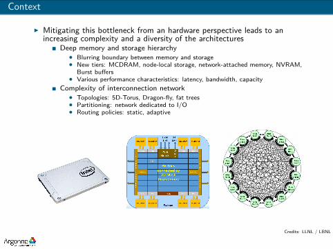
I Mitigating this bottleneck from an hardware perspective leads to anincreasing complexity and a diversity of the architectures

Deep memory and storage hierarchy• Blurring boundary between memory and storage• New tiers: MCDRAM, node-local storage, network-attached memory, NVRAM,

Burst buffers• Various performance characteristics: latency, bandwidth, capacity

Complexity of interconnection network• Topologies: 5D-Torus, Dragon-fly, fat trees• Partitioning: network dedicated to I/O• Routing policies: static, adaptive

Credits: LLNL / LBNL

Data Aggregation

I Selects a subset of processes to aggregate data before writing it to thestorage system

I Improves I/O performance by writing larger data chunksI Reduces the number of clients concurrently communicating with the

filesystemI Available in MPI I/O implementations such as ROMIO

Limitations:I Inefficient aggregator

placement policyI Cannot leverage the deep

memory hierarchyI Inability to use staging

data

X Y Z X Y Z X Y Z X Y Z

Processes

Data

AggregatorsX X X X Y Y

Y Y Z Z Z Z FileX X X X Y Y

Y Y Z Z Z Z

2 - I/O Phase

1 - Aggr. Phase

P0 P1 P2 P3

P0 P2

Figure: Two-phase I/O mechanism

MA-TAPIOCA - Memory-Aware TAPIOCA

I Based on TAPIOCA, a library implementing the two-phase I/O scheme fortopology-aware data aggregation at scale1 and featuring:

Optimized implementation of the two-phase I/O scheme (I/O scheduling)Network interconnect abstraction for I/O performance portabilityAggregator placement taking into account the network interconnect and thedata access pattern

I Augmented to include:Abstraction including the topology and the deep memory hierarchyArchitecture-aware aggregators placementMemory-aware data aggregation algorithm

Memory API

Memory abstractionD

RA

M

HB

M

NV

RA

M

PFS

Application

MA-TAPIOCA

I/O Calls

Destination

Aggr. placement

Topology abstraction

BG/QXC40 ...

...

1F. Tessier, V. Vishwanath, and E. Jeannot. “TAPIOCA: An I/O Library for OptimizedTopology-Aware Data Aggregation on Large-Scale Supercomputers”. In: 2017 IEEE InternationalConference on Cluster Computing (CLUSTER). Sept. 2017.

MA-TAPIOCA - Abstraction for Interconnect Topology

I Topology characteristics include:Spatial coordinatesDistance between nodes: number of hops, routing policyI/O nodes location, depending on the filesystem (bridge nodes, LNET, ...)Network performance: latency, bandwidth

I Need to model some unknowns such as routing in the future

Listing 1: Function prototypes for network interconnecti n t networkBandwidth ( i n t l e v e l ) ;i n t networkLatency ( ) ;i n t networkDistanceToIONode ( i n t rank , i n t IONode ) ;i n t networkDis tanceBetweenRanks ( i n t srcRank , i n t destRank ) ;

Figure: 5D-Torus on BG/Q and intra-chassis Dragonfly Network on Cray XC30(Credit: LLNL / LBNL)

MA-TAPIOCA - Abstraction for Memory and Storage

I Memory management APII Topology characteristics including spatial

location, distanceI Performance characteristics: bandwidth,

latency, capacity, persistencyI Scope of memory/storage tiers (PFS vs

node-local SSD)On those cases, a process has to beinvolved at destination

Memory API (alloc, write, read, free, …)

Abstraction layer (mmap, memkind, …)

DRAM HBM NVRAM PFS ...

MA-TAPIOCA

Listing 2: Function prototypes for memory/storage data movementsbu f f_ t∗ memAlloc (mem_t mem, i n t bu f f S i z e , boo l masterRank ,

char∗ f i l eName , MPI_Comm comm) ;vo id memFree ( bu f f_ t ∗bu f f ) ;i n t memWrite ( bu f f_ t ∗bu f f , vo id∗ s r cBu f f e r ,

i n t s r c S i z e , i n t o f f s e t , i n t destRank ) ;i n t memRead ( bu f f_ t ∗bu f f , vo id∗ s r cBu f f e r ,

i n t s r c S i z e , i n t o f f s e t , i n t s rcRank ) ;vo id memFlush ( bu f f_ t ∗bu f f ) ;i n t memLatency (mem_t mem) ;i n t memBandwidth (mem_t mem) ;i n t memCapacity (mem_t mem) ;i n t memPers i s tency (mem_t mem) ;

MA-TAPIOCA - Memory and topology aware aggregator placement

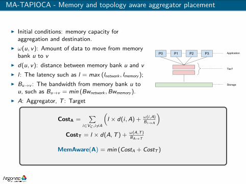
I Initial conditions: memory capacity foraggregation and destination.

I ω(u, v): Amount of data to move from memorybank u to v

I d(u, v): distance between memory bank u and vI l : The latency such as l = max (lnetwork , lmemory );I Bu→v : The bandwidth from memory bank u to

u, such as Bu→v = min (Bwnetwork , Bwmemory ).I A: Aggregator, T : Target

P0 P1 P2 P3 Application

Tier?

Storage

1CostA =∑

i∈VC ,i 6=A

(l × d(i , A) + ω(i,A)

Bi→A

)CostT = l × d(A, T ) + ω(A,T )

BA→T

MemAware(A) = min (CostA + CostT )


CostA =∑

i∈VC ,i 6=A

(l × d(i , A) + ω(i,A)

Bi→A

)CostT = l × d(A, T ) + ω(A,T )

BA→T


HBM

DRAM

P1

DRAM

NVR

HBM

P3

DRAMNVR HBM

P2

DRAMNVR HBM

P0Lustre FS

NVR

1

14 4

3

5

1

2

1

2

41

11

Value# HBM DRAM NVR NetworkLatency (ms) 10 20 100 30

Bandwidth (GBps) 180 90 0.15 12.5Capacity (GB) 16 192 128 N/APersistency No No job lifetime N/A

Table: Memory and network capabilities based on vendors information


CostA =∑

i∈VC ,i 6=A

(l × d(i , A) + ω(i,A)

Bi→A

)CostT = l × d(A, T ) + ω(A,T )

BA→T


1

HBM

DRAM

P1

DRAM

NVR

HBM

P3

DRAMNVR HBM

P2

DRAMNVR HBM

P0Lustre FS

NVR

4

1

2

1

1

Value# HBM DRAM NVR NetworkLatency (ms) 10 20 100 30

Bandwidth (GBps) 180 90 0.15 12.5Capacity (GB) 16 192 128 N/APersistency No No job lifetime N/A

Table: Memory and network capabilities based on vendors information

P# ω(i, A) HBM DRAM NVR0 10 0.593 0.603 2.3501 50 0.470 0.480 2.0202 20 0.742 0.752 2.7103 5 0.503 0.513 2.120

Table: For each process, MemAware(A)

MA-TAPIOCA - Two-phase I/O algorithm

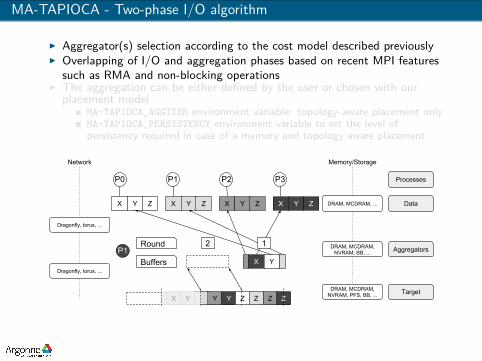
I Aggregator(s) selection according to the cost model described previouslyI Overlapping of I/O and aggregation phases based on recent MPI features

such as RMA and non-blocking operationsI The aggregation can be either defined by the user or chosen with our

placement modelMA-TAPIOCA_AGGTIER environment variable: topology-aware placement onlyMA-TAPIOCA_PERSISTENCY environment variable to set the level ofpersistency required in case of a memory and topology aware placement

Processes

Data

Aggregators

Target

DRAM, MCDRAM, NVRAM, BB, ...

DRAM, MCDRAM, NVRAM, PFS, BB, ...

DRAM, MCDRAM, ...

Dragonfly, torus, ...


Network Memory/Storage


P0 P1 P2 P3

P0 P1 P2 P3





Processes

Data

Aggregators

Target



DRAM, MCDRAM, ...





P0 P1 P2 P3

Buffers

Round 2 1

X Y

X Y Y Y Z Z Z Z

P1





Processes

Data

Aggregators

Target



DRAM, MCDRAM, ...





P0 P1 P2 P3

Buffers

Round 2 1

X Y

X Y Y Y Z Z Z Z

P1

RMA Operations

Non-blocking MPI calls





Algorithm 1: Collective MPI I/O1 n← 5;2 x [n], y [n], z[n];3 ofst ← rank × 3× n;55

6 MPI_File_read_at_all (f , ofst, x , n, type, status);7 ofst ← ofst + n ;99

10 MPI_File_read_at_all (f , ofst, y , n, type, status);11 ofst ← ofst + n;1313

14 MPI_File_read_at_all (f , ofst, z, n, type, status);

Algorithm 2: MA-TAPIOCA1 n← 5;2 x [n], y [n], z[n];3 ofst ← rank × 3× n;55

6 for i ← 0, i < 3, i ← i + 1 do7 count[i ]← n;8 type[i ]← sizeof (type);9 ofst[i ]← ofst + i × n;

1111

12 MA-TAPIOCA_Init (count, type, ofst, 3);1414

15 MA-TAPIOCA_Read (f , ofst, x , n, type, status);16 ofst ← ofst + n ;1818

19 MA-TAPIOCA_Read (f , ofst, y , n, type, status);20 ofst ← ofst + n;2222

23 MA-TAPIOCA_Read (f , ofst, z, n, type, status);

Experiments - Test-beds

ThetaI Cray CX40 11.69 PFlops supercomputer at Argonne

4,392 Intel KNL nodes with 64 cores16 GB of HBM, 192 GB of DRAM and 128 GB on-node SSD

I 10 PB parallel file system managed by LustreI Cray Aries dragonfly network interconnect

Opt. links 12.5 GBps Compute node

Sonnexion storage

Aries router

Knights Landing proc.4 per router

Lustre filesystem

2D all-to-all structure96 routers per group

36 tiles (2 cores, L2)16 GB MCDRAM192 GB DDR4128 GB SSD

Intel KNL 7250Dragonfly network

Elec. links 14 GBps

6 (le

vel 2

)

16 (level 1)

Dragonfly network Compute node

2-cabinet group12 groups - 24 cabinets16 x 6 routers hostedAll-to-all

(leve

l 3)

Service nodeLNET, gateway, … Irregular mapping

210 GBps

CooleyI Intel Haswell-based visualization and analysis cluster at Argonne

126 nodes with 12 cores and a NVIDIA Tesla K80384 GB of DRAM and a local hard drive (345 GB)

I 27 PB of storage managed by GPFSI FDR Infiniband interconnect

Experiments - S3D-IO

S3D-IOI I/O kernel of direct numerical simulation code

in the field of computational fluid dynamicsfocusing on turbulence-chemistry interactionsin combustion.

I 3D domain decompositionI The state of each element is stored in an array

of structure data layoutI The files as output are used for checkpointing

and data analysis Figure: Credits: C.S. Yoo etAl., Ulsan NIST, Republic ofKorea

Experimental setupI Theta, a 11 PFlops Cray XC40 supercomputer with a Lustre filesystem

Single shared file collectively written every n timesteps, stripped amongOST.Available tiers of memory: DRAM, HBM, on-node SSD96 aggregators for 256 nodes and 384 for 1024 nodes for both MPI-IO andMA-TAPIOCALustre: 48 OST, 16MB stripe size, 4 aggr. per OST, 16MB buffer size

I Average and standard deviation on 10 runs

S3D-IO on Cray XC40 + Lustre

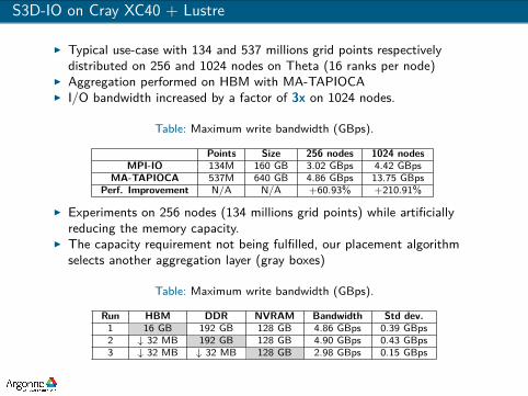
I Typical use-case with 134 and 537 millions grid points respectivelydistributed on 256 and 1024 nodes on Theta (16 ranks per node)

I Aggregation performed on HBM with MA-TAPIOCAI I/O bandwidth increased by a factor of 3x on 1024 nodes.

Table: Maximum write bandwidth (GBps).

Points Size 256 nodes 1024 nodesMPI-IO 134M 160 GB 3.02 GBps 4.42 GBps

MA-TAPIOCA 537M 640 GB 4.86 GBps 13.75 GBpsPerf. Improvement N/A N/A +60.93% +210.91%

I Experiments on 256 nodes (134 millions grid points) while artificiallyreducing the memory capacity.

I The capacity requirement not being fulfilled, our placement algorithmselects another aggregation layer (gray boxes)

Table: Maximum write bandwidth (GBps).

Run HBM DDR NVRAM Bandwidth Std dev.1 16 GB 192 GB 128 GB 4.86 GBps 0.39 GBps2 ↓ 32 MB 192 GB 128 GB 4.90 GBps 0.43 GBps3 ↓ 32 MB ↓ 32 MB 128 GB 2.98 GBps 0.15 GBps

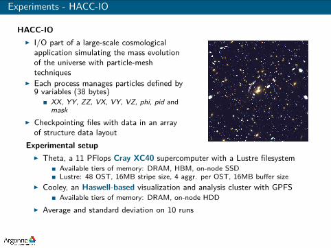
Experiments - HACC-IO

HACC-IOI I/O part of a large-scale cosmological

application simulating the mass evolutionof the universe with particle-meshtechniques

I Each process manages particles defined by9 variables (38 bytes)

XX, YY, ZZ, VX, VY, VZ, phi, pid andmask

I Checkpointing files with data in an arrayof structure data layout

Experimental setupI Theta, a 11 PFlops Cray XC40 supercomputer with a Lustre filesystem

Available tiers of memory: DRAM, HBM, on-node SSDLustre: 48 OST, 16MB stripe size, 4 aggr. per OST, 16MB buffer size

I Cooley, an Haswell-based visualization and analysis cluster with GPFSAvailable tiers of memory: DRAM, on-node HDD

I Average and standard deviation on 10 runs

HACC-IO on Cray XC40 + Lustre

10

100

0 0.5 1 1.5 2 2.5 3 3.5 4

Bandw

idth

(G

Bps)

Data size per rank (MB)

MPI-IO Write on LustreMPI-IO Read on Lustre

MA-TAPIOCA Write on Lustre (Agg: DDR)MA-TAPIOCA Read on Lustre (Agg: DDR)

MA-TAPIOCA Write on SSD (Agg: DDR)MA-TAPIOCA Read on SSD (Agg: DDR)

(a) One file per node on 1024 nodes whilevarying the data size per rank.

0

50

100

150

200

250

300

256 512 1024

I/O

Bandw

idth

(G

Bps)

Number of nodes

MPI-IO WriteMA-TAPIOCA Write

MA-TAPIOCA on SSD WriteMPI-IO Read

MA-TAPIOCA ReadMA-TAPIOCA on SSD Read

(b) One file per node, 1MB/rank, whilevarying the number of nodes.

I Experiments on 1024 nodes on ThetaI Aggregation layer set with the MA-TAPIOCA_AGGTIER environment variableI Regardless of the subfiling granularity, MA-TAPIOCA can use the local

SSD as a shared file destination (mmap + MPI_Win)


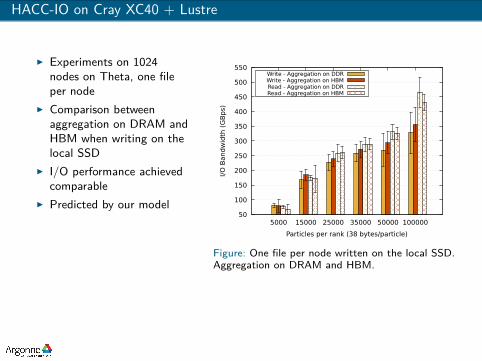
I Experiments on 1024nodes on Theta, one fileper node

I Comparison betweenaggregation on DRAM andHBM when writing on thelocal SSD

I I/O performance achievedcomparable

I Predicted by our model 50

100

150

200

250

300

350

400

450

500

550

5000 15000 25000 35000 50000 100000I/O

Band

wid

th (

GB

ps)

Particles per rank (38 bytes/particle)

Write - Aggregation on DDRWrite - Aggregation on HBMRead - Aggregation on DDRRead - Aggregation on HBM

Figure: One file per node written on the local SSD.Aggregation on DRAM and HBM.


I Typical workflow that can be seamlessly implemented with MA-TAPIOCAI Experiments on 256 nodes on ThetaI Write time counter-balanced by the read time from the local storageI Total I/O time reduced by more than 26%

App

licat

ion

DR

AM

DR

AM

Parallel file

system

Aggregation I/O

Write

Read

SSD

mmap

Table: Max. Write and Read bandwidth (GBps) and total I/O time achieved with andwithout aggregation on SSD

Agg. Tier Write Read I/O timeMA-TAPIOCA DDR 47.50 38.92 693.88 ms

MPI-IO DDR 32.95 37.74 843.73 msMA-TAPIOCA SSD 26.88 227.22 617.46 ms

Variation -36.10% +446.94% -26.82%

HACC-IO on Cooley + GPFS

I Code and performance portability thanks to our abstraction layerI Experiments on 64 nodes on Cooley (Haswell-based cluster)I Same application code, same optimization algorithm using our memory

and network interconnect abstractionI Total I/O time reduced by 12%

App

licat

ion

DR

AM

DR

AM

Parallel file

system

Aggregation I/O

Write

Read

mmap

HDD

Table: Max. Write and Read bandwidth (GBps) and total I/O time achieved with andwithout aggregation on local HDD

Agg. Tier Write Read I/O TimeMA-TAPIOCA DDR 6.60 38.80 123.41 ms

MPI-IO DDR 6.02 17.46 155.40 msMA-TAPIOCA HDD 5.97 35.86 135.86 ms

Variation -0.83% +105.38% -12.57%

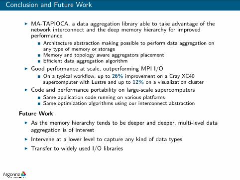
Conclusion and Future Work

I MA-TAPIOCA, a data aggregation library able to take advantage of thenetwork interconnect and the deep memory hierarchy for improvedperformance

Architecture abstraction making possible to perform data aggregation onany type of memory or storageMemory and topology aware aggregators placementEfficient data aggregation algorithm

I Good performance at scale, outperforming MPI I/OOn a typical workflow, up to 26% improvement on a Cray XC40supercomputer with Lustre and up to 12% on a visualization cluster

I Code and performance portability on large-scale supercomputersSame application code running on various platformsSame optimization algorithms using our interconnect abstraction

Future WorkI As the memory hierarchy tends to be deeper and deeper, multi-level data

aggregation is of interestI Intervene at a lower level to capture any kind of data typesI Transfer to widely used I/O libraries

Conclusion

AcknowledgmentsI Argonne Leadership Computing Facility at Argonne National LaboratoryI DOE Office of Science, ASCRI Proactive Data Containers (PDC) project

Conclusion

Thank you for your [email protected]

optimizing data aggregation by leveraging the deep memory

Documents