orah harris onyekachi - dspace.unn.edu.ng
TRANSCRIPT
1
AN ALGORITHM FOR MOBILE LOCATION ESTIMATION IN A 3G NETWORK
BY
ORAH HARRIS ONYEKACHI PG/M.ENG/11/59470
DEPARTMENT OF ELECTRONIC ENGINEERING
FACULTY OF ENGINEERING
UNIVERSITY OF NIGERIA, NSUKKA
APRIL, 2015
APPROVAL PAGE
2
AN ALGORITHM FOR MOBILE LOCATION ESTIMATION IN A 3G NETWORK
ORAH HARRIS ONYEKACHI
(PG/M.ENG/11/59470)
A THESIS SUBMITTED IN PARTIAL FULFILMENT OF THE REQUIREMENTS FOR THE AWARD OF MASTER OF ELECTRONIC ENGINEERING (COMMUNICATION OPTION) IN THE DEPARTMENT OF ELECTRONIC ENGINEERING, UNIVERSITY OF NIGERIA, NSUKKA
ORAH HARRIS ONYEKACHI SIGNATURE…………………DATE……..…………. (STUDENT) PROF C.I. ANI SIGNATURE………………… DATE……..…………. (SUPERVISOR) EXTERNAL EXAMINER SIGNATURE…………………DATE……..………….
Dr. M.A AHANEKU SIGNATURE………………… DATE……..………… (HEAD OF DEPARTMENT) PROF. E.S OBE SIGNATURE……………….. DATE……..…………... (CHAIRMAN FACULTY POSTGRADUATE COMMITTEE)
CERTIFICATION
3
Orah, Harris Onyekachi, a Master’s degree student in the Department of Electronic Engineering andwith registration number PG/M.ENG/11/59470 has satisfactorily completed the requirements for the award of Master of Engineering (M.ENG) in ElectronicEngineering.
………………………………… ..………………………….
PROF. C.I. ANI Dr. M.A AHANEKU (SUPERVISOR) (HEAD OF DEPARTMENT)
…………………………………………………..
PROF. E.S.OBE (CHAIRMAN, FACULTY POSTGRADUATE COMMITTEE)
DECLARATION
4
I, Orah Harris Onyekachi, a postgraduate student of the Department of Electronic Engineering, University of Nigeria, Nsukka declare that the work embodied in this thesis is original and has not been submitted by me in part or in full for other diploma or degree of this or any other University.
Orah Harris DATE PG/M.ENG/11/59470
DEDICATION

5
This work is dedicated to all unrecognized Nigerian engineers who believe in themselves and make genuine efforts to improve indigenous contributions to knowledge through sound research in science and technology.
ACKNOWLEDGEMENT

6
I sincerely acknowledge the insightful directions and guidance from my supervisor, Prof. C.I Ani, which led to the success of this work. I am most grateful to the Almighty God; the ultimate source of knowledge, wisdom and understanding.
OrahHarris. O
7
ABSTRACT
Locating the position of a mobile user with a high degree of accuracy is a trending research
interest. It holds the key to a breakthrough in many service challenges faced by operators in the
wireless communication industry. With a success in this field, it will be possible for call rates in
mobile phones to be charged based on the location a subscriber is calling from; fighting crimes
and delivering emergency services through the mobile network’s ability to detect the caller’s
position will be possible. Many techniques have been proposed or developed for locating the
position of a mobile station in a telecommunication network. Those in operation are mostly
handset-based and each technique has its limitations. These ranged from the degree of accuracy
of the location estimate and response time of the system, to the cost and ease of implementing
the technique. The same goes for the various algorithms employed by these techniques. This
work presents a novel network-based Time Difference of Arrival (TDOA) algorithm for use in
estimating the position of a caller in a 3G mobile network. It is based on geometric principles
and uses known network parameters to calculate the unknown positions of mobile users in the
network. The algorithm improved the accuracy in the estimated position of a mobile user without
incurring the mathematical complexities in hyperbolic trilateration methods conventionally used
by TDOA techniques. From the results of the simulation, the improvement in the accuracy of the
located coordinates of the mobile phone was up to 86.82% and 89.20% for the x and y
coordinates respectively. The method adds no modification in the available cellular infrastructure
and incurs no additional costs.
8
TABLE OF CONTENTS
Title page i
Approval Page ii
Certification iii
Declaration iv
Dedication v
Acknowledgment vi
Abstract vii
List of Figures xi
List of Table xiii
List of Abbreviations xiv
CHAPTER ONE:INTRODUCTION ....................................... Error! Bookmark not defined.
1.1Background of the Study..................................................... Error! Bookmark not defined.
1.2 Problem Statement ............................................................. Error! Bookmark not defined.
1.3 Aim/Objectives .................................................................. Error! Bookmark not defined.
1.5 Scope ................................................................................. Error! Bookmark not defined.
1.6 Methodology ..................................................................... Error! Bookmark not defined.
1.7 Outline of the work.………………………………………………….......……………… ...Error! Bookmark not defined.
CHAPTER TWO:LITERATURE REVIEW ........................... Error! Bookmark not defined.
2.1 Overview of mobile network generations ........................... Error! Bookmark not defined.
2.1.1 The early generation of mobile systems........................... Error! Bookmark not defined.
2.1.2 The first generation (1G) ................................................. Error! Bookmark not defined.
2.1.3 Second Generation (2G) mobile network standards ......... Error! Bookmark not defined.
2.1.4 The 2.5G Network .......................................................... Error! Bookmark not defined.
2.1.5 The Third Generation (3G) network ................................ Error! Bookmark not defined.
2.1.6 High Speed Packet Access (HSPA) ................................. Error! Bookmark not defined.
9
2.1.7: 4G technology standard................................................. Error! Bookmark not defined.
2.1.8 4G Architecture .............................................................. Error! Bookmark not defined.
2.1.9 LTE and WiMAX ........................................................... Error! Bookmark not defined.
2.2 A Review of Mobile Location Estimation Techniques for 3G Networks Error! Bookmark not defined.
2.2.1 Methods for mobile location estimation .......................... Error! Bookmark not defined.
2.3 A Review of literatures on works done in Mobile location estimation .... Error! Bookmark not defined.
2.4 Standalone techniques ........................................................ Error! Bookmark not defined.
2.5 Hybrid techniques .............................................................. Error! Bookmark not defined.
2.6 Summary of the Reviewed Literatures ............................... Error! Bookmark not defined.
CHAPTER THREE:MODELLING ......................................... Error! Bookmark not defined.
3.1 Model specification............................................................ Error! Bookmark not defined.
3.2 System model design ......................................................... Error! Bookmark not defined.
3.2.1 Co-ordinate System Transformation ................................ Error! Bookmark not defined.
3.3 Evaluation technique .......................................................... Error! Bookmark not defined.
3.4 Performance metrics .......................................................... Error! Bookmark not defined.
3.5 Parameters considered in the work: .................................... Error! Bookmark not defined.
3.6 Hyperbolic Equation model and Solution Algorithms ....... Error! Bookmark not defined.
3.6 Hyperbolic Equation model and Solution Algorithms ....... Error! Bookmark not defined.
3.7 Analysis and model design for the algorithm ...................... Error! Bookmark not defined.
3.7.1 The Flow Chat for the algorithm ..................................... Error! Bookmark not defined.
CHAPTER FOUR:SIMULATION AND RESULTS ANALYSIS ........ Error! Bookmark not defined.
4.1 Model Validation ............................................................... Error! Bookmark not defined.
4.2 Simulation of the algorithm................................................ Error! Bookmark not defined.
4.3 Simulation results .............................................................. Error! Bookmark not defined.
4.4 Degree of disparity in the actual and estimated values of the coordinates of the MS for varying positions of a set of three BTS .................................... Error! Bookmark not defined.
4.5 The effect of increasing the number of BTSs on the RMSE in MS distances Measurement ................................................................................................ Error! Bookmark not defined.
4.6 Analysis of the effect of Geometric Dilution of Precision (GDOP) on the accuracy of the algorithm ................................................................................. Error! Bookmark not defined.

10
CHAPTER FIVE:CONCLUSION AND RECOMMENDATIONS ...... Error! Bookmark not defined.
Appendix 1: The MATLAB Script file for executing and simulating the algorithm ......... Error! Bookmark not defined.
References ............................................................................... Error! Bookmark not defined.
11
LIST OF FIGURES
No Name Page
Figure 2.1 1G Cellular network architecture 9
Figure 2.2 2.5G architecture 11
Figure 2.3 UMTS (3G) architecture 13 Figure 2.4 LTE architecture for 4G network 16 Figure 2.5 Architecture of A mobile location service 19
Figure 2.6 The TOA technique 22
Figure 2.7 Angle of Arrival method 24
Figure 2.8 Two-dimensional TDOA position location system 27
Figure 3.1 Mobile location architecture for a 3G network 37
Figure 3.2 Circular Error Probability 49
Figure 3.3 Signal form a mobile user reaching three BTS 53
Figure 3.4 MS is located at the point of intersection of two hyperbolas 55 Figure 3.5 Step 1, the point of intersection of two hyperbolas formed using the
reference NodeBs 56
Figure 3.6 Step 2, the range difference between the two reference nodeBs
is added as an extension, Δd 56
Figure 3.7 Steps for developing the functions used in the algorithm. 57
Figure 4.1 a plot of the real values of the x coordinates of the mobile phone versus the calculated values 63 Figure 4.2 a plot of the real values of y coordinates of the mobile phone versus the calculated values 64
Figure 4.3 Sample MS Location diagram from MATLAB using the Algorithm 65
Figure 4.4 the circular lateration done with 3 BTS 67
12
Figure 4.5 the circular lateration done with 4 BTS 68 Figure 4.6 the circular lateration done with 5 BTS 69 Figure 4.7 the circular lateration done with 6 BTS 69 Figure 4.8 the circular lateration done with 7 BTS 70 Figure 4.9 A comparison of the estimated and actual values of the x- coordinates for a mobile user with different sets of three BSs. 71 Figure 4.10 A comparison of the estimated and actual values of the y- coordinates for a mobile user with different sets of three BSs. 72 Figure 4.11 A comparison of the estimated and actual distance of BTS from MS 73 Figure 4.12 Graph of Root Mean Square error in calculated distance from MS position to the Base stations versus increasing number of BTS 74 Figure 4.13 a set of BTS with bad GDOP 75 Figure 4.14a Bad GDOP 76 Figure 4.14b Shaded region could result from bad GDOP 76 Figure 4.15a Another case of Bad GDOP 77 Figure 4.15b two of the three circles overlap at a parallel. 77
Figure 4.16a Good GDOP 78
Figure 4.16b Good distribution of BTS 78
13
LIST OF TABLES
Table 4.1 Amount of Error in proceeding distance measurements as the number
of BTS increased 66
Table 4.2 Real vs Estimated values of x and y for different positions of MS 66 Table 4.3 varying range difference measurements for constant position of x and y 68
14
LIST OF ABBREVIATIONS
2D Two Dimensional
3D Three Dimensional
1G First Generation
2G Second Generation
3G Third Generation
4G Fourth Generation
ACN Automatic Crash Notification
ADSL Asymmetric Digital Subscriber Line
A-GPS Assisted GPS
AMPS Advanced Mobile Phone System
AOA Angle of Arrival
AMTS - Advanced Mobile Telephone System
AWGN Additive White Gaussian Noise
BTS Base Transceiver Station
CEP Circular Error Probability
CDMA Code Division Multiple Access
CID Cell Identity
CRLB Cramer-Rao Lower Bound
CWLS Constrained Weighted Least Squares
DECT Digital Enhanced Cordless Telecommunications
ECEF Earth-centered Earth fixed co-ordinate system
EDGE Enhanced Data rates for GSM Evolution
E-OTD Enhanced Observed Time of Difference
FCC Federal Communications Commission
FDE Frequency Domain Equalization
FLOPS Floating Point Operations

15
GIS Geographical Information Systems
GDOP Geometric Dilution Of Precision
GDP Geometric Dilution of Position
GPRS General Packet Radio Service
GPS Global Positioning System
GSM Global System for Mobile Communication
GTD Geometric-Time-Difference
HSDPA High Speed Downlink Packet Access
HSPA High Speed Packet Access
HSUPA High Speed Uplink Packet Access
HTAP Hybrid TOA/AOA Positioning
IMTS Improved Mobile Telephone Service
IMT-Advanced International Mobile Telecommunications Advanced
IP Internet Protocol
LBS Location-Based Services
LOS Line-Of-Sight
LMU Location Measurement Unit
MMSE Minimum Mean Square Error
MMS Multimedia Message Service
MS Mobile Station
MTS Mobile Telephone System
MIMO Multiple-Input Multiple-Output
MSE Mean Squared Error
NMR Network Measurements Reports
NLOS Non-Lone-of-Sight
NED North-East Down co-ordinate system
OTDOA Observed Time Difference of Arrival
OFDMA Orthogonal Frequency Division Multiple Access
PDA Personal Digital Assistant
PDC Personal Digital Cellular
PSAP Public Safety Answering Point
16
PTT Push to Talk
QoS Quality of Service
RMSE Root Mean Square Error
RNC Radio Network Controller
RSS Received Signal Strength
RTD Real-Time-Difference
RTT Round Trip Time
SCM Signal Correlation Method
SERP Spherical Error Probability
SIM SubscriberIdentity Module
SRNC Serving Radio Network Controller
TA Timing Advance
TDOA Time Difference of Arrival
TDMA Time Division Multiple Access
TOA Time of Arrival Method
TOAD Time of Arrival to Time Difference of Arrival
TOF Time Of Flight
TTFF Time To First Fit
UE User Equipment
UMTS Universal Mobile Telecommunications System
U-TDOA Uplink Time Difference of Arrival VAS Value Added Service
VoIP Voice over Internet Protocol
W-CDMA Wideband Code Division Multiple Access
WGS World Geodetic Systems
WiMax Worldwide Interoperability for Microwave Access

17
18
CHAPTER ONE
INTRODUCTION
1.1 Background of the Study
The problem of providing reliable and accurate position location of mobile devices in wireless
communication systems has attracted a lot of attention in recent years. The adoption of
regulations by Federal Communications Commission (FCC) in the U.S has been the main force
pushing research interests in mobile position location [1]. In 1996, the USA Federal
Communications Commission (FCC) issued a mandate to wireless service providers to grant that
a mobile unit calling the emergency number 911 can be located with accuracy within 125 meters
of its actual position in 67% of all calls, and 300 meters for 95% of calls in all cases [1]. This
was called the enhanced 911 services. The FCC’s wireless 911 rules seek to improve the
reliability of wireless 911 services and to provide emergency services personnel with accurate
location information that will enable them to locate and provide assistance to wireless 911 callers
much more quickly. The ruling required that by October 1st, 2001 all mobile operators should
provide the Public Safety Answering Point (the emergency call centre) with the geographic
position of phones that make 911 wireless emergency calls within 50–100meters[1]. The location
of the mobile should be presented in the 2D or 3D coordinate or in longitude and latitudes.
Although the FCC requirements where not entirely met in October 2001 and many extensions
and waivers have been granted by the FCC to telecommunication operators, the Enhanced-911
(E-911) mandate inspired a lot of research works and technology developments in mobile
location estimation. It also spawned an entirely new industry for location-aware applications,
formally named location-based services (LBS) [2].
Over the years, researchers have studied mobile location estimation with a goal of finding a
solution that is cost effective, easy to implement, compatible with existing core network
infrastructure and offers a high degree of accuracy. The most widely developed of the mobile
location estimation solutions is the Global positioning system (GPS) [2], which is based on
signals transmitted from satellites in space. The GPS is highly accurate but requires the addition
of some non-standard features either in the mobile terminal or the network, which brings
19
additional cost on the equipment manufacturers. Though GPS is fitted in many recent GSM
handsets, its effective use in location estimation is still hampered by some factors.
One of such factors is the requirement of a clear view of the sky to receive GPS signals from at
least three satellites out of the 24 geolocation satellites in space. This makes the system
inefficient in urban areas with tall buildings, and in areas surrounded by mountains and other
obstructions [1].
Thus, research works have intensified on developing improved mobile location systems that use
Radio frequency signals as found in GSM networks, since these signals are not obstructed like
the satellite signals. With such solutions the user’s location must be determined from data that is
inherently present in the cellular network. The data comprises network parameters such as the
serving-cell identity, signal strength, timing advance and neighboring cell measurement [3].
These data can be used in many ways to determine the position of a mobile in a GSM network.
One of such ways is the Angle of Arrival (AOA) method which uses sector information from the
serving BTS. Another method uses signal propagation time in the form of Timing Advances
(TA). The Time Difference of Arrival (TDOA) method is a more widely applied method having
several advantages over the previous methods. The TDOA method is successfully applied in the
cellular network[4]. This work developeda geometric algorithm that uses TDOA measurements
and range difference equations tocalculate the position of a mobile station (MS) in a 3G network.
Though algorithms have been developed that used TDOA and range difference measurements to
make location estimates for a mobile device, they are iterative, prone to error and
computationally intensive. Using a geometric approach offers less computational complexity and
improves accuracy in location estimates.
However, there exist many incentives for wireless service providers to have such a system in
place. They can use reliable position location as a means to optimize the performance and design
of the wireless networks and can also offer additional features to the subscribers.
Position location services will not only provide new customer options and products for wireless
carriers, but will also provide features that could differentiate services in different markets (i.e.,
differentiation between PCS, cellular, and specialized mobile radio) [5]. Location systems will
also provide wireless carriers and vendors, who use position location, the ability to charge for
service based on location. This could be within a particular cell site, or in a specific location such
as an office, home, or car. This will allow wireless service providers to control customer usage
20
by offering cost incentives that match service plans for the wireless infrastructure and
networking resources.
Geographical information about the service usage will also enable the service to have real-time
information about areas having concentration of usage and such information will facilitate
cellular planning. It will also be easier to locate the sources of fraudulent cellular telephone
traffic and fraud emergency calls and thus the business loss which results from fraud can be
reduced. Location information of mobile users can also be used to increase the hand-off
efficiency in cellular networks. Design of efficient hand-off algorithms is an important issue in
cellular design, and position location information may help in avoiding unnecessary hand-offs
that may result because of local fading and hence may help reduce the processing load[6, 7]
Knowledge of the position of a caller in a mobile network is also of great benefits to the
individual using the mobile phone. Automated position determination will also help in providing
emergency road-side services quickly and efficiently, especially in the case of an accident.
Position location systems may also be very helpful for companies in fleet management and can
be used for traffic routing and scheduling of vehicles in real time [5]. There can also be a number
of potential applications of position location systems for in-car navigation systems and for
direction finding from known position to given destinations.Apart from the above cited
advantages, law enforcement agencies may benefit considerably from such systems which may
be used to increase their crime fighting capability [5].Real-time position location may be used to
track the location of officers and agents. Such information may also be used to track suspected
criminals and to recover stolen vehicles.
1.2 Problem Statement The full deployment of location aware services is still a problem to mobile communication
operators. Due to the poor degree of accuracy, cost of implementation, complexity of network
infrastructure and modification needed on the existing handsets to run this new feature, many
proposed solutions could not be implemented. Some existing methods fail to offer the same level
of accuracy for different environments[8]. Purely Network–based location estimation methods
21
that use radio frequency signals are not yet fully developed and widely accepted. In the existing
methods that incorporate the network in estimating the location of a mobile device, the role of
the network is usually to provide assistance in the form of computation or some parameters when
the GPS has got the required signals; and where these signals are obstructed by buildings or
trees, these methods fail [1].
Among the stand alone methods proposed for measuring the location of a mobile user is the time
difference of arrival (TDOA) technique. This technique measures the difference in the arrival
time of signals from the Mobile Station (MS) at some base stations (uplink) in the network[9]. It
relies on hyperbolic trilateration which is a range difference method, and requires at least 2 pairs
of base stations to make an estimate of the position of a caller in a network. The range difference
between the other base stations receiving signal from the MS with respect to the reference base
station will be obtained by transforming TDOAs into range difference measurements [9]
It is the central focus of location estimation algorithms that use the TDOA methods.
The performance and results of the algorithms for solving this equation vary depending on the
geometrical configuration of the base stations, and the number of coordinates of the mobile’s
position to be solved.
1.3 Aim/Objectives
The main aim of this work is to develop an improved algorithm that usesTDOA measurements
and coordinate geometric principles to locate with good accuracy the position of a mobile device
in a 3G cellular network.
Therefore, the objectives of this work are as follows:
• To improve on the network- based TDOA algorithm for computing the 2-D coordinates
of a mobile station in a 3G network without introducing the need for modification to the
existing handsets and network infrastructure.
• To improve the accuracy of location estimation technologies that use the TDOA
techniques and reduce the computational complexities in the use of this technique.
22
• To develop an algorithm that can be used by location based service application
developers in deploying emergency services and other location aware services in a
mobile telecommunication network.
1.4 Significance of the study
Wireless geolocation has a great number of applications called location-based services, which
can be defined as value added services that utilize the knowledge of the mobile user's
geographical location. Developing an easy method for calculating the positions of mobile
devices is helpful and essential for a great number of reasons.
.
In military applications for instance, an accurate location estimation technology can enable
Command and Control Centers to track the positions of their units, an injured soldier or a
vehicle. The same applies to companies in fleet management and vehicular navigations.
The monitored entities would have the capacity to transmit necessary location finding signals
which would be used in order to provide the geographic location information and render
assistance where it is needed.
A reliable location finding algorithm could also be of benefit in rendering roadside assistance.
Examples of services that come under this are personal direction finding, mapping, navigation
assistance and traffic information. Questions such as “Where is the nearest filling station?" or “I
lost my way, how can I get to Abuja?" could be readily answered by the mobile network
providers using mobile location technologies.
Tracking for both people such as children, seniors, mentally handicapped and car or asset could
be made possible through position location technologies.
Other location based services that could be made possible by this technology include:
• Crime fighting
• Automatic Crash Notification (ACN), which reports a crash of an automobile to
necessary places, such as fire and PSAP (Public Safety Answering Point)
• Location-based billing
23
• Location specific information such as local weather, mobile yellow pages, mobile
directory assistance, etc. and
• Mobile e-commerce, wireless advertising and instant messaging
A successful location estimation technique will open new opportunities for delivering value-
added services; new investments in location based service provision and subsequently create
more revenue for Mobile technology operators.
1.5 Scope
The work focuses on locating the 2D coordinates of a mobile phone user in a 3G cellular
network. TDOA values are calculated from data generated on a test map of the distribution of
base stations in a 3G cellular network drawn to scale. The algorithm is simulated using a
MATLAB script file. For all the instances of the application of the algorithm during the
simulation, the mobile user in the cellular network is stationary.
1.6 Methodology
The research work started with a wide review off related literatures and works done by other
people in failed of mobile location estimation. Through the review a need for an improved
algorithm for mobile location estimation was identified. A new algorithm was proposed for
locating the 2-D coordinates of a mobile phone. The algorithm was modeled using the MATLAB
software. A validation for the algorithm was done by comparing the results from MATLAB
simulations to the actual coordinates of known positions of a mobile phone from a test map.
Then analysis for the results was made, while a recommendation for areas for further studies was
given also.
1.7 Outline of the work
The organization of this project is as follows:
Chapter one presents the background of the research, and its aim/objectives. It highlights the
existing problems, outlines the research objectives, its significant and scope.
24
Chapter two reviews related literatures to the subject of mobile location estimation.
In Chapter three, the methodology, design and system modeling approach used in this work were
presented.
Chapter four focuses on the analysis of the results obtained from the simulation of the algorithm
Chapter five summarizes the research findings and makes recommendations on the project.

25
CHAPTER TWO
LITERATURE REVIEW
2.1 Overview of mobile network generations
A generation of a mobile network refers to a change in the fundamental nature of the mobile
network services. It marks an introduction of a non-backwards-compatible transmission
technology, higher peak bit rates, use of new frequency bands, wider channel frequency
bandwidth in Hertz, and higher capacity for many simultaneous data transfers (higher system
spectral efficiency in bit/second/Hertz/site) [10]. On a simple note, each Generation of mobile
telecommunication network is defined as a set of telephone network standards, which details the
implementation of the technology supporting a specific mobile phone system. Each generation
have some standards, capacities, techniques and new features which differentiate it from
previous generations [10]
2.1.1 The early generation of mobile systems Earlymobile radio systems used a single, high-powered transmitter with an antenna mounted on a
tall tower to cover a large service area (e.g. a city) [11]. This approach in the design of a mobile
radio system had the limitations of poor use of scarce wireless spectrum. The system also had
limited capacity in the sense that only a very few number of mobile users can communicate
simultaneously through a voice call. Bell mobile system in New York City, as an example, in
the 1970s could only support a maximum of 12 calls simultaneously over thousand square miles
[12]. Mobile phones used under this system needed to have a very high transmitting power to be
able to cover a considerable distance within the radio antenna service area. The cellular concept
was introduced to overcome these problems [12]. The concept proposed a replacement of the
high power transmitters with many lower power transmitters, each covering only small portion of
the service area called a cell. This gave birth to the cellular network.
26
2.1.2 The first generation (1G) This generation of wireless telecommunication technology is popularly known as cell
phones[13]. This set of wireless standards were developed in the 1980's, and replaced the early
generation technology, which featured mobile radio telephones and such technologies as Mobile
Telephone System (MTS), Advanced Mobile Telephone System (AMTS), Improved Mobile
Telephone Service (IMTS), and Push to Talk (PTT).
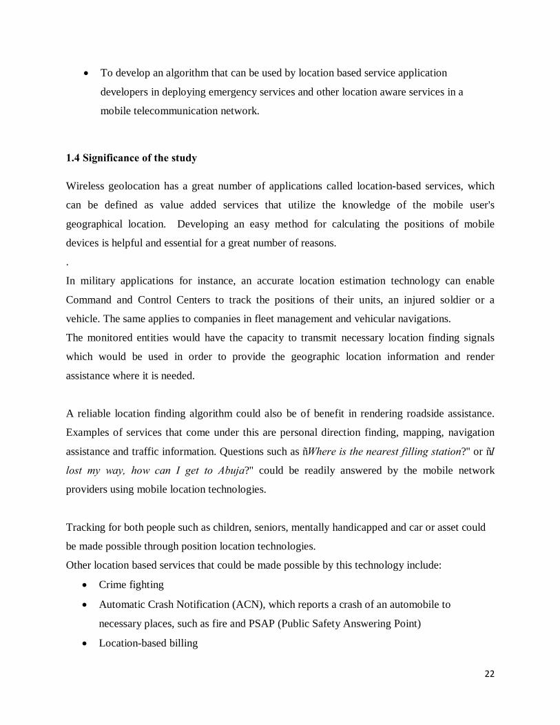
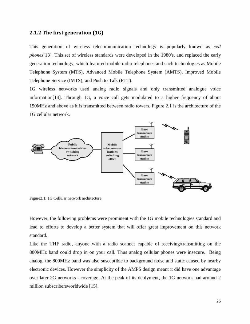
1G wireless networks used analog radio signals and only transmitted analogue voice
information[14]. Through 1G, a voice call gets modulated to a higher frequency of about
150MHz and above as it is transmitted between radio towers. Figure 2.1 is the architecture of the
1G cellular network.
Figure2.1: 1G Cellular network architecture
However, the following problems were prominent with the 1G mobile technologies standard and
lead to efforts to develop a better system that will offer great improvement on this network
standard.
Like the UHF radio, anyone with a radio scanner capable of receiving/transmitting on the
800MHz band could drop in on your call. Thus analog cellular phones were insecure. Being
analog, the 800MHz band was also susceptible to background noise and static caused by nearby
electronic devices. However the simplicity of the AMPS design meant it did have one advantage
over later 2G networks - coverage. At the peak of its deplyment, the 1G network had around 2
million subscribersworldwide [15].

27
2.1.3 Second Generation (2G) mobile network standards Security issues and network congestion problems were the major motivations for the
development of the 2G standards[16]. These challenges marred the successful operation of the
1G network standards and technologies. The development of 2G cellular systems was further
driven by the need to improve transmission quality, system capacity, and coverage. Introduced
in early 1990s, the new technology was purely digital and came with many new services and
capabilities that extended those of the 1G mobile systems, while still overcoming their
limitations. Further advances in semiconductor technology and microwave devices brought
digital transmission to mobile communications as used in the 2G network.This new digital
network is popularly called GSM - Global System for Mobile Communication and its
technological backbone of choice is TDMA (in Europe) and CDMA (in US)[17]. Other 2G
systems, of similar scale, include the Japanese personal digital cellular (PDC) and the TIA time
division multiple access (TDMA) used mainly in the Americas. The CDMA version of the 2G
technology is referred to as cdmaOne.
2G network allows for much greater penetration intensity of wireless services. 2G technologies
enabled the various mobile phone networks to provide the services such as text messages, picture
messages and MMS (multimedia messages). All text messages sent over 2G are digitally
encrypted, allowing for the transfer of data in such a way that only the intended receiver can
receive and read it. In a GSM system, unlike in analog mobile networks, subscription and
mobile equipment are separated. Subscriber data are stored and handled by a SubscriberIdentity
Module (SIM), which is a smart card belonging to a subscriber. When thinking of the services,
the most remarkable difference between 1G and 2G is the presence of a data transfer possibility;
basic GSM offers 9.6 kb/s symmetric data connection between the network and the terminal [18].
The 2G technologies recorded the following improvements in the GSM technology [13,15 ]. The
FDMA component splits the 900MHz (actually 890MHz to 915MHz) band into 124 channels
that are 200 KHz wide. The 'time' component (TDMA) then comes into play in which each
channel is split into eight 0.577us bursts, significantly increasing the maximum number of users
at any one time. Aside from more users per cell tower, the digital network offers many other
important features:
- digital encryption (64bit A5/1 stream cipher)
28
- packet data (used for MMS/Internet access)
- SMS text messaging
- caller ID and other similar network features.
However, unlike its AMPS predecessor, GSM is limited severely in range. The TDMA
technology behind the 2G network means that if a mobile phone cannot respond within its given
timeslot (0.577us bursts) the phone tower will drop the call and begin handling another call[19].
Aside from this, packet data transmission rates on GSM are extremely slow. To overcome these
problems, one of the networks introduced was the CDMA (Code Division Multiple Access).
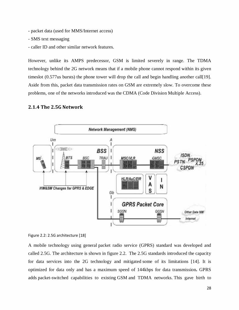
2.1.4 The 2.5G Network
Figure 2.2: 2.5G architecture [18]
A mobile technology using general packet radio service (GPRS) standard was developed and
called 2.5G. The architecture is shown in figure 2.2. The 2.5G standards introduced the capacity
for data services into the 2G technology and mitigated some of its limitations [14]. It is
optimized for data only and has a maximum speed of 144kbps for data transmission. GPRS
adds packet-switched capabilities to existing GSM and TDMA networks. This gave birth to
29
emails which comprises texts and graphics-rich data sent as packets at very fast speed over the
internet. The circuit-switched technology has a long and successful history but it is inefficient
for short data transactions and always-on service as is the case with GSM network.
In a GPRS system, each mobile terminal is assigned an IP address. The assignment can be static,
as determined by the cellular operator, or else dynamic, on a per connection basis. When the
mobile terminal is on, it is always connected to GPRS. The mobile subscriber is charged for the
amount of data transferred, not on a time basis as done for voice calls[20].
2.1.5 The Third Generation (3G) network The evolution towards third generation cellular systems (3G) was driven by the need for higher
capacity, faster data rates, and better quality –of –service (QoS). Also prominent was the desire
to define a new system that resolved many incompatibilities between the different standards,
mainly GSM (Europe) and CDMAone (US), so as to facilitate, for example, mobile roaming
between the different systems. The 3G allows for more coverage and growth with minimum
investment [21].
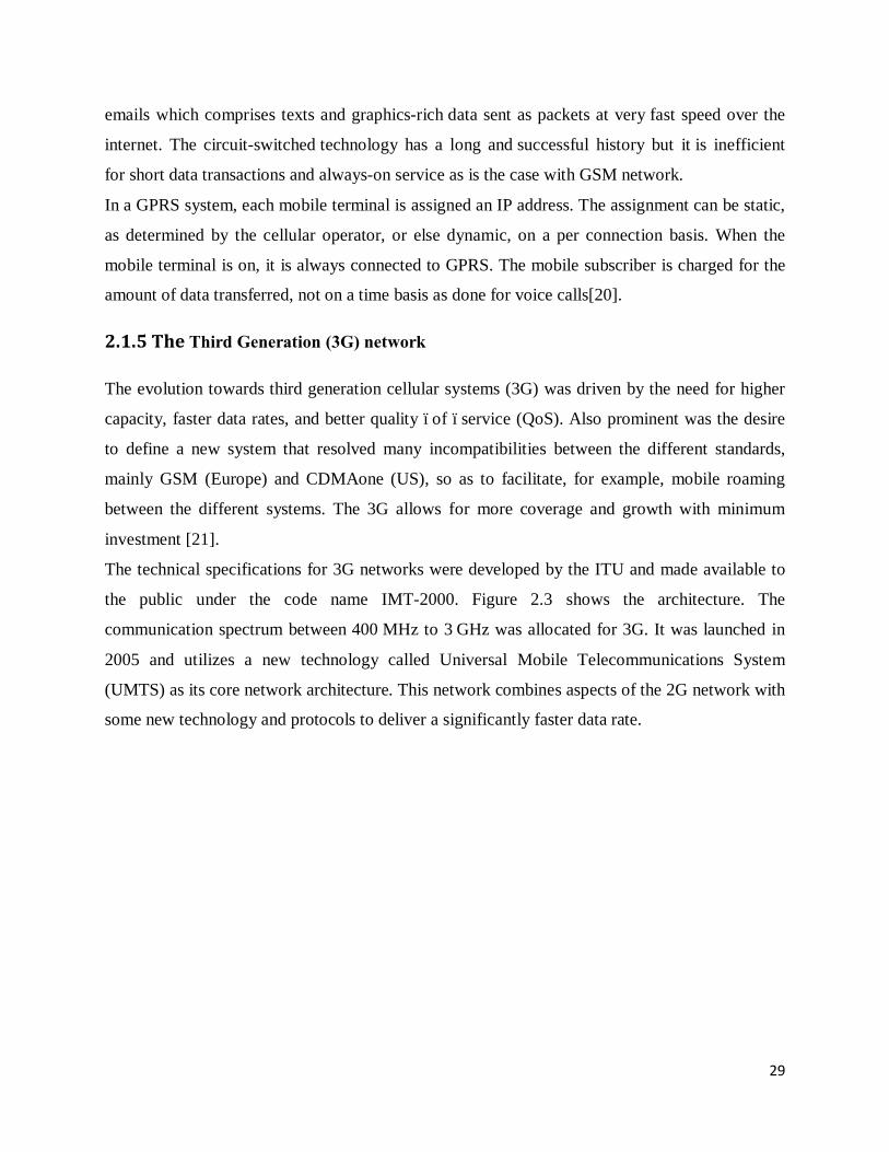
The technical specifications for 3G networks were developed by the ITU and made available to
the public under the code name IMT-2000. Figure 2.3 shows the architecture. The
communication spectrum between 400 MHz to 3 GHz was allocated for 3G. It was launched in
2005 and utilizes a new technology called Universal Mobile Telecommunications System
(UMTS) as its core network architecture. This network combines aspects of the 2G network with
some new technology and protocols to deliver a significantly faster data rate.
30
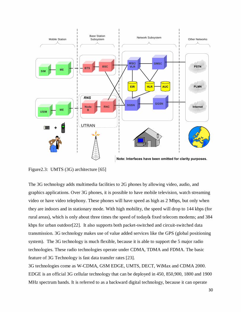
Figure2.3: UMTS (3G) architecture [65]
The 3G technology adds multimedia facilities to 2G phones by allowing video, audio, and
graphics applications. Over 3G phones, it is possible to have mobile television, watch streaming
video or have video telephony. These phones will have speed as high as 2 Mbps, but only when
they are indoors and in stationary mode. With high mobility, the speed will drop to 144 kbps (for
rural areas), which is only about three times the speed of today’s fixed telecom modems; and 384
kbps for urban outdoor[22]. It also supports both packet-switched and circuit-switched data
transmission. 3G technology makes use of value added services like the GPS (global positioning
system). The 3G technology is much flexible, because it is able to support the 5 major radio
technologies. These radio technologies operate under CDMA, TDMA and FDMA. The basic
feature of 3G Technology is fast data transfer rates [23].
3G technologies come as W-CDMA, GSM EDGE, UMTS, DECT, WiMax and CDMA 2000.
EDGE is an official 3G cellular technology that can be deployed in 450, 850,900, 1800 and 1900
MHz spectrum bands. It is referred to as a backward digital technology, because it can operate
SD
Mobile Station
MSC/VLR
Base StationSubsystem
GMSC
Network Subsystem
AUCEIR HLR
Other Networks
Note: Interfaces have been omitted for clarity purposes.
GGSNSGSN
BTS BSC
NodeB
RNC
RNS
UTRAN
SIM ME
USIMME
+
PSTN
PLMN
Internet
31
with older devices. EDGE allows for faster data transfer than existing GSM. while EDGE do not
meet all the objectives of a 3G system, EDGE offers significant higher data rates compared to
GPRS [24].
2.1.6High Speed Packet Access (HSPA)
This is an upgrade for UMTS networks that doubles network capacity and increases download
data speeds by five times or more. The service was initially deployed at 1.8 Mbps but upgrades
to the networks and new user devices led to increased rates of 3.6 Mbps, followed by 7.2 Mbps
and further down the road, 14.4Mbps and even 21Mbps [25]. HSDPA (High Speed Downlink
Packet Access) only handles the downlink while the uplink is handled by a related technology
called (High Speed Uplink Packet Access) HSUPA. The combination of both technologies is
usually called HSPA (High Speed Packet Access). It was this technology that allowed users of
3G phones to really use the Internet on their mobile phones send pictures and watch streaming
video at usable speeds [25].
HSDPA is a new protocol for mobile telephone data transmission. It is known as a 3.5G
technology. Essentially, the standard will provide download speeds on a mobile phone equivalent
to an ADSL (Asymmetric Digital Subscriber Line) line in a home, removing any limitations
placed on the use of your phone by a slow connection. It is an evolution and improvement on W-
CDMA. HSDPA improves the data transfer rate by a factor of at least five over W-CDMA.
HSDPA can achieve theoretical data transmission speeds of 8-10 Mbps (megabits per second.
Though any data can be transmitted, applications with high data demands such as video and
streaming music are the focus of HSDPA [26].
2.1.7: 4G technology standard 4G refers to IMT-Advanced (International Mobile Telecommunications Advanced) standard for
mobile telecommunication. The IMT-Advanced cellular system was intended to fulfill the
following requirements[27]:
• Be based on an all-IP packet switched network.

32
• Have peak data rates of up to approximately 100 Mbit/s for high mobility such as mobile
access and up to approximately 1 Gbit/s for low mobility such as nomadic/local wireless
access.
• Be able to dynamically share and use the network resources to support more
simultaneous users per cell.
• Using scalable channel bandwidths of 5–20 MHz, optionally up to 40 MHz.
• Have peak link spectral efficiency of 15 bit/s/Hz in the downlink, and 6.75 bit/s/Hz in the
uplink (meaning that 1 Gbit/s in the downlink should be possible over less than 67 MHz
bandwidth).
• System spectral efficiency of up to 3 bit/s/Hz/cell in the downlink and 2.25 bit/s/Hz/cell
for indoor usage.
• Smooth handovers across heterogeneous networks.
• The ability to offer high quality of service for next generation multimedia support
As opposed to earlier generations, a 4G system does not support traditional circuit-switched
telephony service. It is designed as a data-only network such that all of the traffic is IP-based as
is the case with IP telephony. One of the major differences - besides the faster speeds - between
these networks and 3G is that voice - which until now travelled over a separate line – will now
run over the same network as the data, and telephony on the phone basically becomes a
VoIP[28].
Also the spread spectrum radio technology used in 3G systems is abandoned in all 4G candidate
systems. The multiple access scheme for the 4G physical layer is based on Orthogonal
Frequency Division Multiple Access (OFDM) with a Cyclic Prefix (CP) in the downlink and a
Single Carrier Frequency Division Multiple Access (SC-FDMA) with CP in the uplink.
OFDMA technique is particularly suited for frequency selective channel and high data rate [29].
It transforms a wideband frequency selective channel into a set of parallel flat fading narrowband
channels, due to the presence of CP. This makes it possible to transfer very high bit rates despite
extensive multi-path radio propagation (echoes).
The final important feature is the use of multi-antenna techniques (MIMO) and Coordinated
Multi Point (CoMP) to provide more capacity and more consistent data rates across cell
boundaries. In other words, it will be possible to maintain a more consistent download rate as a
33
user move in and out of the range of transmitters.With speeds of over 100 Mbps, wireless
networks can easily rival the speeds of wired connections [30, 31]. Thanks to this, areas where it
is currently too expensive to update wired networks may soon get access to real broadband. By
doing away with the enormous costs of physically connecting every household to the wired
networks, hopefully more competition will be seen among Internet providers.
Faster speeds are not just the only advantage of these networks. The latency - that is the time it
takes the network to respond to a request - is also greatly reduced over these networks.
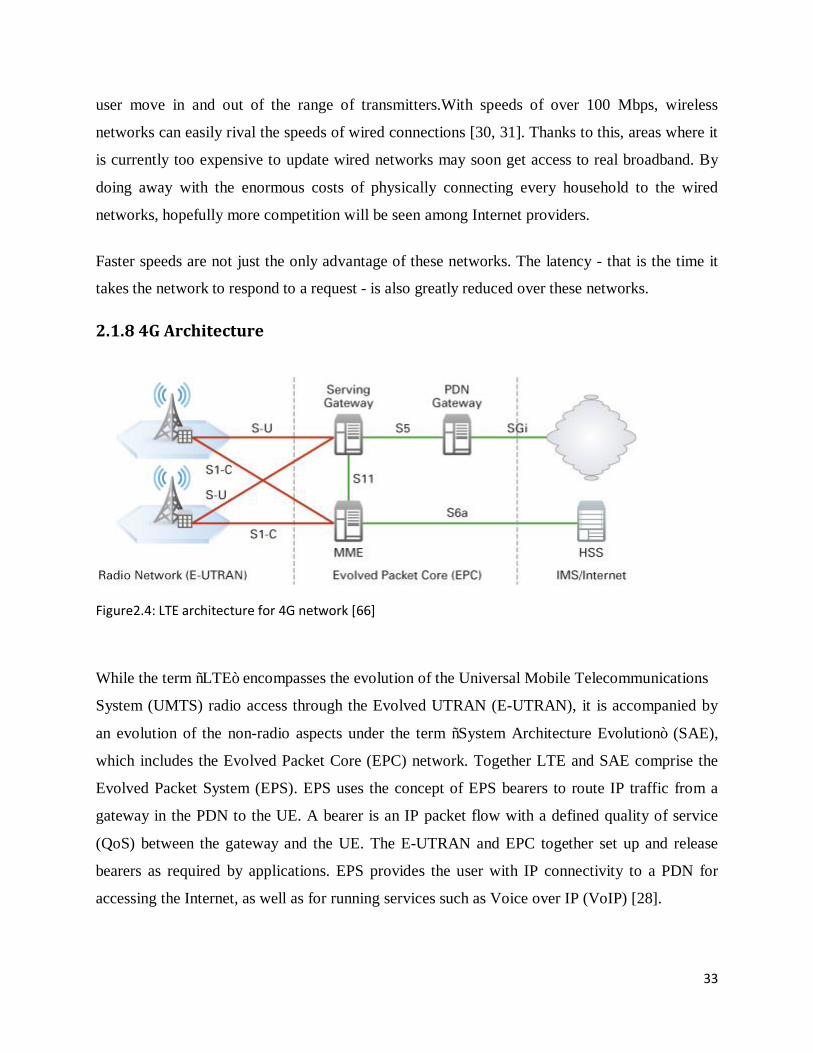
2.1.8 4G Architecture
Figure2.4: LTE architecture for 4G network [66]
While the term “LTE” encompasses the evolution of the Universal Mobile Telecommunications
System (UMTS) radio access through the Evolved UTRAN (E-UTRAN), it is accompanied by
an evolution of the non-radio aspects under the term “System Architecture Evolution” (SAE),
which includes the Evolved Packet Core (EPC) network. Together LTE and SAE comprise the
Evolved Packet System (EPS). EPS uses the concept of EPS bearers to route IP traffic from a
gateway in the PDN to the UE. A bearer is an IP packet flow with a defined quality of service
(QoS) between the gateway and the UE. The E-UTRAN and EPC together set up and release
bearers as required by applications. EPS provides the user with IP connectivity to a PDN for
accessing the Internet, as well as for running services such as Voice over IP (VoIP) [28].
34
An EPS bearer is typically associated with a QoS. Multiple bearers can be established for a user
in order to provide different QoS streams or connectivity todifferent PDNs. For example, a user
might be engaged in a voice (VoIP) call while at the same time performing web browsing or FTP
download. EPS also supports interworking and mobility (handover) with networks using other
Radio Access Technologies (RATs), notably Global System for Mobile Communications
(GSM), UMTS, CDMA2000 and WiMAX.
The core network (called EPC in SAE) is responsible for the overall control of the UE and establishment of the bearers. The main logical nodes of the EPC are:
• PDN Gateway (P-GW)
• Serving Gateway (S-GW)
• Mobility Management Entity (MME)
In addition to these nodes, EPC also includes other logical nodes and functions such as the Home
Subscriber Server (HSS) and the Policy Control and Charging Rules Function (PCRF). Since the
EPS only provides a bearer path of a certain QoS, control of multimedia applications such as
VoIP is provided by the IP Multimedia Subsystem (IMS), which is considered to be outside the
EPS itself.
The logical CN nodes are discussed in more detail below [17]:
• PCRF – The Policy Control and Charging Rules Function is responsible for policy control
decision-making, as well as for controlling the flow-based charging functionalities in the Policy
Control Enforcement Function (PCEF), which resides in the P-GW. The PCRF provides the QoS
authorization (QoS class identifier [QCI] and bit rates) that decides how a certain data flow will
be treated in the PCEF and ensures that this is in accordance with the user’s subscription profile.
• HSS – The Home Subscriber Server contains users’ SAE subscription data such as the EPS
subscribed QoS profile and any access restrictions for roaming. It also holds information about
the PDNs to which the user can connect. This could be in the form of an access point name
(APN) (which is a label according to DNS naming conventions describing the access point to the
PDN) or a PDN address (indicating subscribed IP address(es)). In addition the HSS holds
dynamic information such as the identity of the MME to which the user is currently attached or
35
registered. The HSS may also integrate the authentication center (AUC), which generates the
vectors for authentication and security keys.
• P-GW – The PDN Gateway is responsible for IP address allocation for the UE, as well as QoS
enforcement and flow-based charging according to rules from the PCRF. It is responsible for the
filtering of downlink user IP packets into the different QoS-based bearers. This is performed
based on Traffic Flow Templates (TFTs). The P-GW performs QoS enforcement for guaranteed
bit rate (GBR) bearers. It also serves as the mobility anchor for interworking with non-3GPP
technologies such as CDMA2000 and WiMAX® networks.
• S-GW – All user IP packets are transferred through the Serving Gateway, which serves as the
local mobility anchor for the data bearers when the UE moves between eNodeBs. It also retains
the information about the bearers when the UE is in the idle state (known as “EPS Connection
Management — IDLE” [ECM-IDLE]) and temporarily buffers downlink data while the MME
initiates paging of the UE to reestablish the bearers. In addition, the S-GW performs some
administrative functions in the visited network such as collecting information for charging (for
example, the volume of data sent to or received from the user) and lawful interception. It also
serves as the mobility anchor for interworking with other 3GPP technologies such as general
packet radio service (GPRS) and UMTS.
• MME – The Mobility Management Entity (MME) is the control node that processes the
signaling between the UE and the CN. The protocols running between the UE and the CN are
known as the Non Access Stratum (NAS) protocols.
2.1.9 LTE and WiMAX
The Long Term Evolution (LTE) network and WiMAX are two standards that are often referred
to as 4G standards. Implementations of Mobile WiMAX and LTE do not match up to the full
specifications for 4G in spectra efficiency, download speed, etc, and are thus considered as
stopgap solutions. According to a report by Rysavy Research for 3G Americas [32], the first
networks that will actually fulfill these official requirements for 4G will probably use the LTE-
Advanced specificationsandWiMAX 2 (based on the 802.16m spec). These advanced versions
will represent the true 4G technology standards.
36
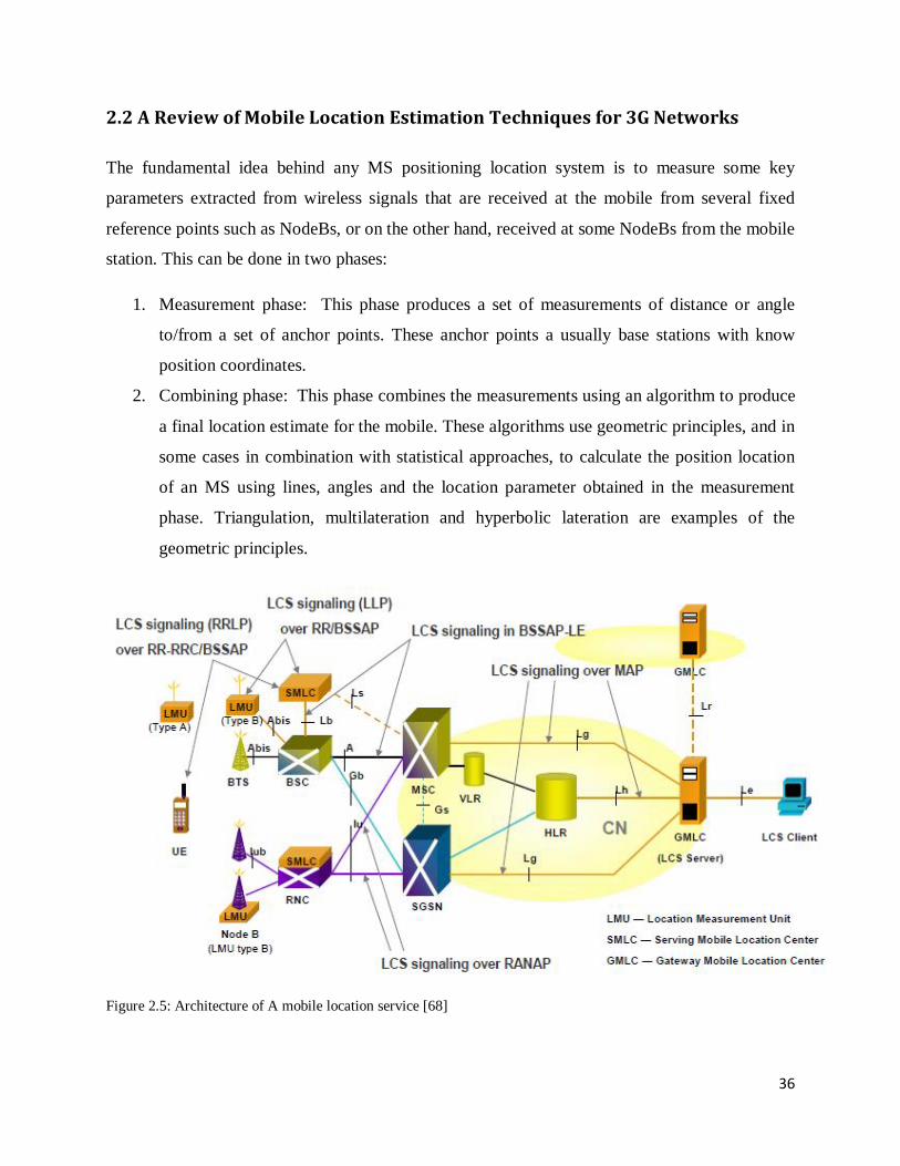
2.2 A Review of Mobile Location Estimation Techniques for 3G Networks The fundamental idea behind any MS positioning location system is to measure some key
parameters extracted from wireless signals that are received at the mobile from several fixed
reference points such as NodeBs, or on the other hand, received at some NodeBs from the mobile
station. This can be done in two phases:
1. Measurement phase: This phase produces a set of measurements of distance or angle
to/from a set of anchor points. These anchor points a usually base stations with know
position coordinates.
2. Combining phase: This phase combines the measurements using an algorithm to produce
a final location estimate for the mobile. These algorithms use geometric principles, and in
some cases in combination with statistical approaches, to calculate the position location
of an MS using lines, angles and the location parameter obtained in the measurement
phase. Triangulation, multilateration and hyperbolic lateration are examples of the
geometric principles.
Figure 2.5: Architecture of A mobile location service [68]
37
This work focuses on the 3G network because it has the Location Measurement Unit built into it.
This entity gives it the ability to measure signal parameters like TDOA, which are used in the
location estimation algorithm. Furthermore, The GSM technology is the most widely used
cellular technology and 3G is the most widely used advanced form of it.
2.2.1 Methods for mobile location estimation A mobile position location system consists of at least two hardware components; a measuring
unit that usually carries the main part of the system and a signal transmitter. The function of the
transmitter in the simplest case is just to send beacon signals. According to the place in which the
position location calculation is executed, these systems can mainly be categorized into three
groups: handset-based positioning, network-based positioning, and hybrid-positioning system.
In network-based technologies, the cellular network uses the signals transmitted between it and
the Mobile Station and calculates the position of the MS using those signals. The Cell-Id method,
the Time of Arrival method (TOA), the Time Difference of Arrival (TDOA), the Angle of
Arrival (AOA) and the data base correlation method all fall under the Network-based
technologies [33].Handset-based geolocation technologies are based on the signal transmitted
between satellites in the orbit or base stations in a network, and a mobile device on earth. Using
this approach, the Mobile station calculates its own position using signals it receives either from
base stations or GPS [35]. The GPS and the Observed Time Difference of Arrival (OTDOA)
location techniques fall under this category.
Hybrid solutions combine the network-based and handset-based technologies. The overall idea
behind this approach is to overcome the disadvantages of handset and network based
technologies i.e., limited availability of GPS in some environments and low accuracy of network
based technologies [36]. Wireless Assisted GPS (A-GPS) and Enhanced Observed Time of
Difference (E-OTD) are mobile location techniques in this category.
These technologies can further be distinguished based on those using only the available
infrastructure without any changes to the handset or wireless infrastructure and those actually
requiring some changes. The former class of methods includes the Cell Identity (CID) in which
position location is carried out by finding the cell (geographical coverage area of a base station)
38
the mobile is currently in. If an MS is located in a cell, Cell ID will return the coordinates of the
Base Station as position for the MS. On the other hand if sectorized antennas are used, Cell ID
will return the center of the sector as position [37]. In the Cell ID based method in 3G networks,
the Serving Radio Network Controller (SRNC) determines the identification of the cell providing
coverage for the target User Equipment (UE). If the UE is in a state where the cell ID is
available, the target cell ID is chosen as the basis for the UE Positioning. In states where the cell
ID is not available, the UE is paged, so that SRNC can establish the cell with which the target
UE is associated [37].
Another approach uses the timing advance (TA), which is based on measuring the round-trip
propagation delay of the signal transmitted from the base station to the handset and back to the
base station. This approach does not require improvements on the network infrastructure and
allows the user, given the speed of radio waves, to determine the distance between the base
station and the mobile device [38]. When several base stations were used in this process, the
location of the mobile device is determined as the intersection of the underlying range circles.
RTT (Round Trip Time) is a similar technique to TA and is used in UMTS to enhance the
positioning process. The RTT value is the time difference between the start of a down-link frame
and the reception of the corresponding uplink frame. The accuracy achievable with this
technique can be even higher when compared to TA used in GSM [38].
On the other hand, in the class which requires changes in cellular infrastructure, one finds
methods that are based on the Time of Arrival (TOA), time difference of arrival (TDOA) and
angle of arrival (AOA) of signals.
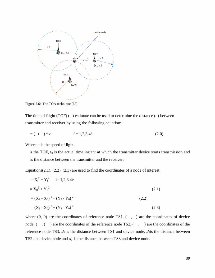
The TOA technique assumes that the MS clock is synchronized with the base station transceivers
(BTS) which serves as nods, and uses an estimate of the time of arrival of the MS signal at the
base stations to calculate the distance of the MS from the reference node. The TOA for two or
more nodes is then combined using multilateration principles to obtain a location estimate for the
MS as shown in figure 2.6. Here if the distances from the reference nodes to the target object T
are known, then the point of the intersection of the three circles formed by these distances is the
supposed location of object T [38].
39
Figure 2.6: The TOA technique [67]
The time of flight (TOF) (��) estimate can be used to determine the distance (d) between
transmitter and receiver by using the following equation:
�� = (��–��) * c i = 1,2,3,4… (2.0)
Where c is the speed of light,
�� is the TOF, t0 is the actual time instant at which the transmitter device starts transmission and
�� is the distance between the transmitter and the receiver.
Equations(2.1), (2.2), (2.3) are used to find the coordinates of a node of interest:
��� = Xi
2 + Yi2 i= 1,2,3,4…
���= X0
2 + Y02 (2.1)
��� = (X2 - X0) 2 + (Y2 - Y0) 2 (2.2)
��� = (X3 - X0) 2 + (Y3 - Y0) 2 (2.3)
where (0, 0) are the coordinates of reference node TS1, (��,��) are the coordinates of device
node, (��, (�� ) are the coordinates of the reference node TS2, (��, ��) are the coordinates of the
reference node TS3, d1 is the distance between TS1 and device node, d2is the distance between
TS2 and device node and d3 is the distance between TS3 and device node.
40
These equations (2.1), (2.2) and (2.3) can be solved by combining all the available set of
measurements using a least-squares approach into a more accurate estimate. This method
assumes that all transmitters and receivers are perfectly synchronized in time and ignores
reflections or interference that will affect the position accuracy.
Time of Arrival is also used by the GPS, where each GPS receiver is synchronized to the atomic
clocks in the satellites for a very precise range measurement [39]. However, the mobile
terrestrial network is normally not synchronized with the MS which leads to rather poor accuracy
for mobile network-based location estimation approaches that utilize this technique.
The AOA approach measures the angle at which uplink signal from a MS arrives at two or three
base stations. Knowing the position of the base stations, lines marking these angles are extended
and their point of intersection gives the possible location of the MS [40]. It is purely network-
based, since the MS does not take part in the measurement nor in the calculation phases. The MS
is only participating by emitting a signal. The basic idea is to steer in space a directional antenna
beam until the direction of maximum signal strength or coherent phase is detected. In terrestrial
mobile systems the directivity required to achieve accurate measurements is obtained by means
of antenna arrays.
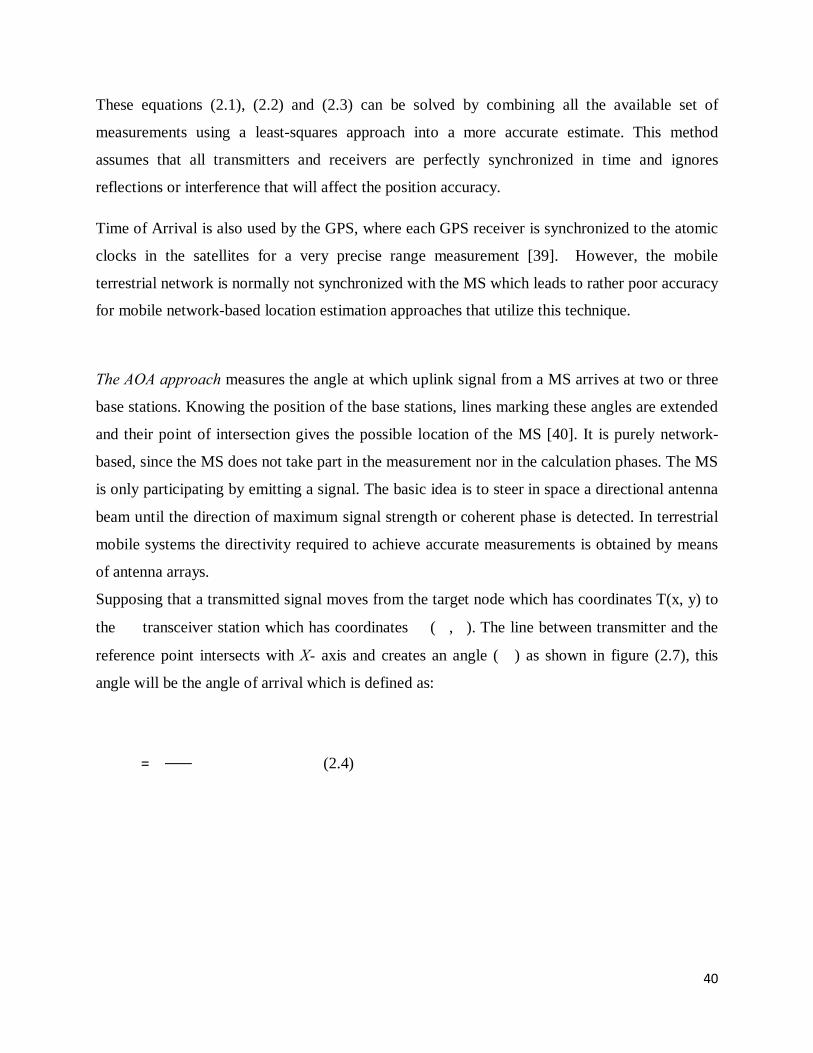
Supposing that a transmitted signal moves from the target node which has coordinates T(x, y) to
the ��� transceiver station which has coordinates ��(��,��). The line between transmitter and the
reference point intersects with X- axis and creates an angle (��) as shown in figure (2.7), this
angle will be the angle of arrival which is defined as:
����� = ���������
� (2.4)

41
Figure2.7: Angle of arrival method
To determine the coordinates of the target node T, the following equations are used:
� = ����(��)�����������(��)
(2.5)
� = �������� ��� (��)����������� (��)
(2.6)
Where R is the distance between the reference stations N1 and N2, ϕ1 is the angle of arrival at the
reference node N1, ϕ2 is the angle of arrival at the reference node N2, (x, y) are the coordinates of
the target node T.
The intersection of the lines represents the assumed position of the MS. The position is not as
accurate as shown on figure2.7 since the measured angle by the antennas is often afflicted with
an error. To obtain good results with this technique the MS should have a clear line-of-sight
(LOS) to the antenna and the distance between these components should not be too great.
Unfortunately in urban areas there is often no clear LOS and in rural areas the distance is mostly
too great. Multipath propagation is another problem of this technique, i.e. signals received with
the most strength could be reflected signals that resulted from multipath effects, thus leading to
false positioning data because they arrive at the BTS under a false angle [41]. This is another
reason why AOA works poorly in urban area. AOA can be used in both GSM and UMTS
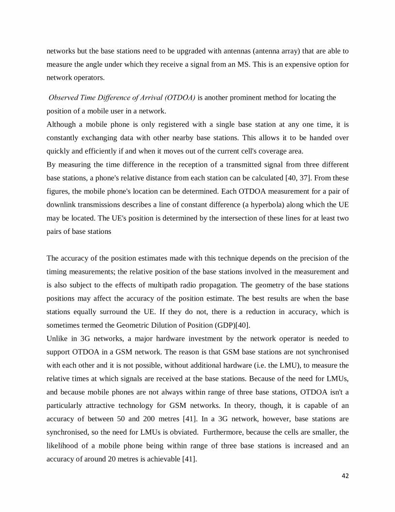
42
networks but the base stations need to be upgraded with antennas (antenna array) that are able to
measure the angle under which they receive a signal from an MS. This is an expensive option for
network operators.
Observed Time Difference of Arrival (OTDOA) is another prominent method for locating the
position of a mobile user in a network.
Although a mobile phone is only registered with a single base station at any one time, it is
constantly exchanging data with other nearby base stations. This allows it to be handed over
quickly and efficiently if and when it moves out of the current cell's coverage area.
By measuring the time difference in the reception of a transmitted signal from three different
base stations, a phone's relative distance from each station can be calculated [40, 37]. From these
figures, the mobile phone's location can be determined. Each OTDOA measurement for a pair of
downlink transmissions describes a line of constant difference (a hyperbola) along which the UE
may be located. The UE's position is determined by the intersection of these lines for at least two
pairs of base stations
The accuracy of the position estimates made with this technique depends on the precision of the
timing measurements; the relative position of the base stations involved in the measurement and
is also subject to the effects of multipath radio propagation. The geometry of the base stations
positions may affect the accuracy of the position estimate. The best results are when the base
stations equally surround the UE. If they do not, there is a reduction in accuracy, which is
sometimes termed the Geometric Dilution of Position (GDP)[40].
Unlike in 3G networks, a major hardware investment by the network operator is needed to
support OTDOA in a GSM network. The reason is that GSM base stations are not synchronised
with each other and it is not possible, without additional hardware (i.e. the LMU), to measure the
relative times at which signals are received at the base stations. Because of the need for LMUs,
and because mobile phones are not always within range of three base stations, OTDOA isn't a
particularly attractive technology for GSM networks. In theory, though, it is capable of an
accuracy of between 50 and 200 metres [41]. In a 3G network, however, base stations are
synchronised, so the need for LMUs is obviated. Furthermore, because the cells are smaller, the
likelihood of a mobile phone being within range of three base stations is increased and an
accuracy of around 20 metres is achievable [41].

43
The GPS technique uses a constellation of 24 satellites that orbit the earth in space and send
signals to a GPS receiver providing precise details of the receiver's location, the time of day, and
the speed the device is moving in relation to the satellites [2]. A GPS receiver (usually installed
in the MS) uses trilateration (a more complex version of triangulation) to determine its position
on the surface of the earth by timing signals from at least three satellites in the Global
Positioning System.
Each satellite in the GPS constellation sends out periodic signals along with a time signal. These
are received by GPS devices, which then calculate the distance between the device and each
satellite based on the delay between the time the signal was sent and the time when it was
received. The signals travel at the speed of light, but there is a delay because the satellites are at
an altitude of tens of thousands of kilometers above the earth. Once a GPS device has distances
for at least three satellites, it can perform the trilateration calculationswhichprovide the position
of the MS in terms of latitude and longitude coordinates with an accuracy of less than 10 metres.
However, usually such estimation is only possible if there is a clear line-of-sight to at least four
GPS satellites. This reduces its capability in case of dense urban-like environment or indoor
environment [42].
The Uplink Time Difference of Arrival (U-TDOA)
The difference between the U-TDOA and TDOA is that in the former the measurement is done
by the network using the uplink signals from the UE to the base stations, whereas in the latter the
measurement is done at the UE using signals from the base stations to the UE. The U-TDOA
approach utilizes hyperbolic lateration (TDOA) principles and is standardized by 3GPP (3rd
Generation Partnership Project) for UMTS and GSM [43].
U-TDOA technology locates wireless phones by comparing the time it takes a mobile station’s
radio signal (Uplink signal) to reach several Location Measurement Units (LMUs) installed at an
operator’s base stations. It is called Uplink-TDOA because the frames in the uplink, from the MS
to the BS and the LMUs, are used to determine the position of the MS. The differences in the
arrival times of this signal are converted into range difference measurements between two or
more base stations. The range difference between two receivers is determined by measuring the
44
difference in time of arrival of a signal between them. The intersection of the hyperbolas
describing these range differences gives an estimate of the location of the MS.
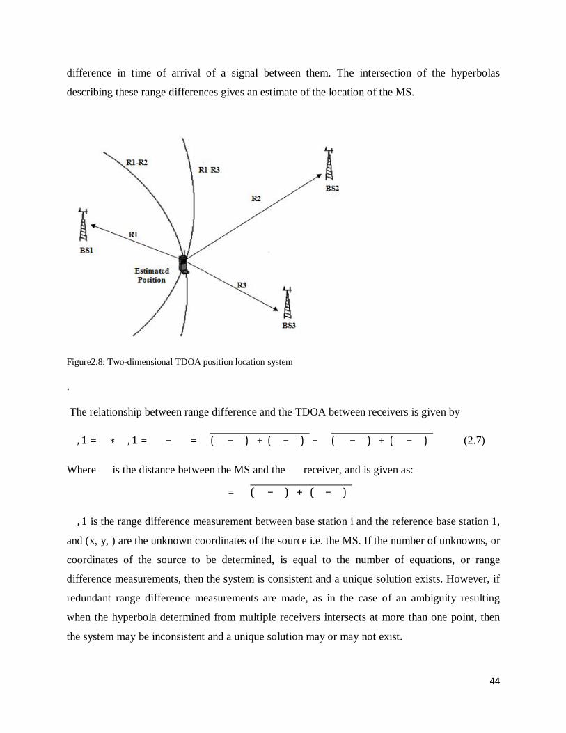
Figure2.8: Two-dimensional TDOA position location system . The relationship between range difference and the TDOA between receivers is given by ��, 1 = �∗ ��, 1 = ��− �� = �(��− �)� + (��− �)� − �(�� − �)� + (�� − �)� (2.7)
Where �� is the distance between the MS and the ��� receiver, and is given as:
�� = �(��− �)� + (��− �)�
��, 1 is the range difference measurement between base station i and the reference base station 1,
and (x, y, ) are the unknown coordinates of the source i.e. the MS. If the number of unknowns, or
coordinates of the source to be determined, is equal to the number of equations, or range
difference measurements, then the system is consistent and a unique solution exists. However, if
redundant range difference measurements are made, as in the case of an ambiguity resulting
when the hyperbola determined from multiple receivers intersects at more than one point, then
the system may be inconsistent and a unique solution may or may not exist.
45
Equation (2.7) is a set of nonlinear hyperbolic equations whose solution gives the 2-D
coordinates of the MS’s location. However, solving this nonlinear equation is difficult.
Consequently, linearizing this equation is commonly performed before applying the algorithms
to estimate the MS’s position.
For U-TDoA, at least 3 BSs are necessary to obtain an unambiguous position and precise
synchronization of base stations is required for this technique to work. LMUs (Location
Measurement Units) have to be deployed in the network to gain this synchronization. Another
prerequisite is that the MS is in busy mode (whether it is a real call or stimulated by the network
to transmit for a short time).
In the U-TDOA method the processing functions to calculate user position is done in the network
equipment, especially location measurement unit (LMU), instead of mobile equipment
processing used in downlink (OTDOA) method. In addition, uplink method has increased
processing capacity available to analyze signal information and to calculate subscriber locations.
The uplink method provides increased power from 20 to 30 dB greater in processing gain than a
downlink OTDOA solution through long integration times [43]. In the downlink OTDOA
system, the mobile station must make measurements of pilot signals from several sites, one by
one, while still providing the other mobile station functions. The DSP processors of many LMUs
work simultaneously to locate a single mobile subscriber. So, downlink method latency problem
is solved. The best results in this method can be obtained in urban areas or areas with dense BS
coverage.
The accuracy of the position estimates made with this technique depends on the precision of the
timing measurements; the relative position of the BTSs used and is also subject to the effects of
multipath radio propagation. No specific hardware support, either hardware or software, is
required in the mobile phone.
A major advantage of the TDOA method is that it does not require knowledge of the transmit
time from the source, as do TOA methods. Consequently, strict clock synchronization between
the source and receiver is not required. As a result, hyperbolic position location techniques do
not require additional hardware or software implementation within the mobile unit. However,
clock synchronization is required of all receivers used for the Position Location estimate.

46
Fingerprinting, also known as Pattern Matching or DatabaseCorrelation, is another approach
used to locate the position of an MS. It uses a measurement of the signal strength received
(RSS) by the MS from the base station, and a propagation model to transform this measurement
into distance from the MS to related BTSs. RSS ranging is based on the principle that the greater
the distance between two wireless nodes is, the weaker their relative received signals are [44].
However, the relationship between the RSS values and the distance depends on a large number
of unpredictable factors. In fact, small changes in position or direction may result in dramatic
differences in RSS values. The RSS values can be modeled by the following expression:
��� = ���� − 10�����������+ �� (3.9)
Where ��is the actual distance between the MS and the anchor;����is the power measured at a
reference distance and it depends on several factors: averaged fast and slow fading, antennas
gains, and transmitted power. In practice, ���� can be often known beforehand and its value will
be valid as long as the antenna gains and the transmitted power remain constant. The term �� is
the path-loss exponent corresponding to the path connecting the MS to the anchor, while
denotes a zero mean Gaussian random variable caused by slow fading [44].
This technique isdivided in two phases: training and the positioning. In thetraining phase or
offline phase, the goal is to build up a database with fingerprintsof reference points in the desired
area where localizationshould take place. The network needs certain informationfrom the MS in
order to make handover decisions(called Network-Measurements Reports - NMR). Therefore at
these reference pointsthe MS measures the signal strength of the serving cell andthe six strongest
surrounding BSs. This measurement is stored in avector. This vector is the fingerprint for one
certain point andis stored in a database within the network. The positions of these fingerprints
were determined byGPS or some other accurate localization technique. The closer thesereference
points are to each other, the better is the accuracybut the higher is the computing time.
In the positioning phase or the online phase, the MS measures the signal strengthfrom the
location where it is and transmits this vector to thedatabase in the network. There, the vector is
compared to theentries with an appropriate search algorithm and the databasereturns the location
which best correlates with the vector.Therefore the returned location is likely to be the
47
positionwhere the MS is [8]. Since both the MS and the network areused, this approach is called
mobile-assisted. It can be usedin GSM, UMTS and WiFi networks and neither changes to the
MS nor changes tothe network have to be made. The problem is that the mentioned seven
element vectorhardly ever is the same for one position. This is among otherthings due to weather
conditions or changes in the area (newbuildings or the like). It is also very time consuming
andexpensive to make all these measurements for a whole city
[45].
2.3 A Review of literatures on works done in Mobile location estimation Reviewed literatures recognized several different kinds of measurements for performing location
estimation. Traditionally, these are angular, distance and time measurements made with respect
to a group of reference points, usually the base stations. A location estimate is then derived using
basic geometry.
2.4 Standalone techniques N. Deligiannis et al presented a novel algorithm for the implementation of TOA location position
technique in GSM networks using three base stations[47]. In order to determine the mobile
station’s position, the algorithm makes use of the Turin’s TOA positioning algorithm. The
proposed approach requires modifications in GSM protocols LAPD, RR and MM as well as the
insertion of a new LAPD layer 3 Paging Command message (Single Paging Command).
Furthermore, an additional weight coefficient in TOA cost function was also proposed. The
additional weight coefficient reflects the LOS/nLOS propagation. The coefficient demands BS
antenna arrays and a GIS map available, but has showed good reduction of the location error due
to NLOS propagation. The extra requirements for the implementation of this technique make it
difficult for deployment in location estimation by mobile network operators.
Sravanthi proposed another method that emphasizes the importance of RSS measurements in
position location and the need to reduce implementation cost in location positioning technologies
[48]. The work presents a new simple approach to finding MS position using Received Signal
Strength (RSS) measurements and is based on pdf of RSS probability method.The method
48
produced improved accuracy and reduction in minimum mean square error (MMSE). It was of
great benefit and enhanced location estimation accuracy. Through this method it is possible to
apply high-performance mobile positioning in a practical and cost effective manner [48].
In an extension of the study on mobile location estimation, a technique called Signal Correlation
Method (SCM), based on Artificial Neural Network was introduced [49]. The new technique is
aimed at achieving the following goals:
a.) developing a method to be utilized when timing measurements are unavailable from 2 or
more Node Bs.
b.) a technique to be used when LBS requests are huge and suitable for continuous query from
Navigation Based Services.
c.) a technique suitable for urban, suburbs and rural (in rural only one omni directional serving
cell is available and Node Bs are very distant from each other), while meeting FCC E-911
location accuracy requirement for network based positioning. SCM technique proved to be
accurate even though using just one cell’s signal level. This is due to using anew process to train
data samples.
An effective method for dynamic location estimation by Kalman Filter for range-based wireless
network was introduced in [50]. In the work, Kalman Filter with TDOA technique describes the
ranging measurement tracking approach. Kalman filter is used for smoothing range data and
reducing the NLOS errors. The paper presents a simple recursive model by using time difference
of arrival based location measurement and incorporating state equality constraints in the Kalman
filter. The proposed recursive locating algorithm, compared with a Kalman tracking algorithm
that estimates the target track directly from the TDOA measurements, will be comparatively
more robust to measurement errors because it updates the technique that feeds the location
corrections back to the Kalman Filter. It compensates for the measured geometrical location and
decreases random error influence to the location precision. Simulation results show that the
proposed location estimation algorithm can improve the accuracy significantly. Furthermore, a novel lookup table correlation technique for geolocation, with multiple position
estimations and optimal location techniques was proposed [51]. The approach they used in the
49
work provides high precise location and tracking of mobile terminals by exploiting advanced
propagation models for mobile radio networks design, and by querying Geographical
Information Systems (GIS) database covering the area of interest, in conjunction with Kalman
predictive filtering. The work relies on additional information extracted from a GIS database
covering the area of interest, used in conjunction with advanced predictive filtering.
Three non-iterative techniques were presented for localizing a single source given a set of noisy
range-difference measurements[52]. The localization formulas are derived from linear least-
squares "equation error" minimization. Geometric interpretations of the equation error norms
minimized by the three methods were given, and the statistical performances of the three
methods were compared through the results from computer simulation.
Two algorithms were developed for accurate mobile location using the time-of-arrival
measurements of the signal from the mobile station received at three or more base stations [53].
The first algorithm is an unconstrained least squares (LS) estimator that is very simple to
implement. The second algorithm solves a non-convex constrained weighted least squares
(CWLS) problem for improving estimation accuracy. Results from simulations showed that the
CWLS estimator yields better performance than the LS method and achieves both the Crame´r-
Rao lower bound and the optimal circular error probability at sufficiently high signal-to-noise
ratio conditions.
However, most standalone location techniques, in spite of their ease of use and other advantages,
still suffer from lack of a clear Line-Of –Sight signals when they are deployed for use in certain
areas. Issues like hearability, latency and degree of accuracy also come up. In order to deal with
these problems, build on the strengths of some of the mobile location methods and compensate
for the weakness of others, hybrid location estimation techniques have been developed. A hybrid
positioning technique is merely one in which multiple techniques are combined for positioning
purposes.

50
2.5 Hybrid techniques The combination of the mobile network and GPS positioning techniques gave rise to the idea of
Assisted-GPS (A-GPS). The basic idea in A-GPS is to enforce a fruitful combination between
Cellular network technology and GPS signals where an assistant server, which can be made
available via, for instance, a network, helps the GPS receiver to perform the tasks required to
determine position estimate [42].
The A-GPS has been acknowledged as a promising technology for future location based systems.
A-GPS enhances the performance of the standard GPS in devices connected to the cellular
network and provides a higher accuracy of mobile location.
A-GPS has the following improved prosperities compared to standard GPS method:
• Higher position accuracy.
• Lower power consumption at GPS receiver terminal.
• Higher receiver sensitivity.
• Lower TTFF and acquisition time.
• Fewer number of satellites needed in position detection[54].
The hybrid TOA/AOA positioning schemes have been proposed for hearability-constrained
environments. The proposed hybrid scheme uses combinations of TOA and AOA measurements
to estimate MS location when only three BSs are available for location purposes. The position of
the MS is found at the intersections of three circles and a line of TOA measurements from three
BSs when the AOA information at the serving BS is available. The proposed schemes reduces
the NLOS effect simply by the weighted sum of the intersections between three TOA circles and
an AOA line without a priori information about the NLOS errors [55].This location method also
gives a good degree of location accuracy for wideband code division multiple access (WCDMA)
systems used in 3G networks standards. High location accuracy can be achieved if line-of-sight
(LOS) propagation exists between the MS and all BSs.The Non-Line-Of-Sight (NLOS)
situations, which generally occur in urban or suburban areas, greatly degrade the precision of this
location estimation scheme.
51
SanemKabadayi and IbrahimTekin proposed a hybrid location finding technique based on time
difference of arrival (TDOA) with round-trip time (RTT) measurements for a wideband code
division multiple access (WCDMA) network [56]. In this technique, a mobile station measures
timing from at least three base stations using user equipment receive–transmit (UERx– Tx) time
difference and at least three base stations to measure timing from the mobile station using RTT.
The timing measurements of mobile and base stations are then combined to solve for both the
location of the mobile and the synchronization offset between base stations.
The time of arrival (TOA) and angle of arrival (AOA) errors in four typical cellular
environments were analyzed and modeled[57]. Based on the analysis results, a hybrid
TOA/AOA positioning (HTAP) algorithm, which utilizes TOA and AOA information delivered
by serving base station,was proposed. The result of simulating the performance of the proposed
algorithm showed that when the MS is close to the serving BS, HTAP will produce an accurate
location estimate. When MS is far from the serving BS, the location estimate obtained by HTAP
can be used as an initial location in their system to help a least square (LS) algorithm converge
easily. When there are more than three TOA detected, weights and TOA numbers used in the LS
algorithm have to be dynamically adjusted according to the distance between MS and serving BS
and the propagation environment. This is done to get a better positioning performance from the
algorithm.
A positioning algorithm named time of arrival to time difference of arrival (TOAD) has been
developed [58]. It computes time-difference-of-arrival (TDOA) measurements from the
messages that time-of-arrival (TOA) stations in sight exchange while their positioning processes
are running. It is aimed at extending the capabilities of the two-way TOA techniques (i.e., those
based on round-trip-time or RTT) and addresses the accuracy of the TOAD algorithm in two
different environments: line-of-sight (LOS) and non-line-of-sight (NLOS). Software Simulation
was used to set up a wireless network while the Gauss-Newton nonlinear least squares algorithm
was used to compute the positions in both TOA and TOAD stations. Results indicate that the
TOAD algorithm increases the root mean square error (RMSE) of the positioning error in LOS
scenarios by 10 to 20% compared with the RMSE achieved by TOA. This drop in accuracy
contrasts with the results for the NLOS scenarios. The RMSE of TOAD in such scenarios is at
least 10% lower than that achieved by TOA. This novel technique improved the scalability and
52
integrity of TOA techniques based on RTT, and made it possible for the stations to position
themselves without injecting traffic and with QoS figures close and most times better than that
achieved by TOA [58].
A method of constrained weighted least squares (CWLS) mobile positioning approach which
comprises most of the mobile location estimation techniques discussed has also been proposed
[59]. According to the report presented on the method, the advantages of CWLS include
performance optimality and capability of extension to hybrid measurement cases (e.g., mobile
positioning using TDOA and AOA measurements at the same time). Assuming zero-mean
uncorrelated measurement errors, mean and variance analysis results show that all the developed
CWLS location estimators achieve zero bias and the Cramér-Rao lower bound approximately
when measurement error variances are small.
2.6 Summary of the Reviewed Literatures
The various techniques and algorithms used for estimating the position of a mobile phone in a
3G wireless network were studied. Also various works done by researchers in the field of mobile
location estimation were also studied. The goal of these studies is to examine the performance of
those methods in terms of degree of accuracy, cost of implementation, ease of implementation
and computational complexities of the methods. Of all the techniques considered, the GPS offers
the best accuracy and is the most widely used for location estimation.
Once a GPS device has distances for at least three satellites, it can perform the trilateration
calculationswhichprovide the position of the MS in terms of latitude and longitude coordinates
with an accuracy of less than 10 meters. However, usually such estimation is only possible if
there is a clear line-of-sight to at least four GPS satellites. The GPS uses satellite signals which
can be obstructed by tall buildings and trees. This reduces its overall performance in cases of
dense urban-like environmentsor indoor environments. The location estimation procedure in this
method is handset-based and does not give the operator much leverage to extensively deploy
LBS and other location-based VAS.
The methods presented in [47, 55, 57, 58] are based on TOA and AOA measurements or a
combination of both. These methods are hampered by non-LOS components of the signaland
53
require additional network infrastructure for their implementation. The measurement of angle
requires additional hardware and antenna arrays to be installed in the network at additional costs.
If more than three angle measurements are available, they are not necessarily compatible due to
angle measuring errors. The TOA technique also requires the mobile station to be synchronized
with the serving BTS. It is thus non realizable in a 3G network where such synchronization and
other requirements cannot be met.
The Received Signal strength measurement is another technique with a good prospect in mobile
location estimation. It uses a measurement of the signal strength received (RSS) by the MS from
the base station, and a propagation model to transform this measurement into distance from MS
to related BTS. It however requires additional hardware and incurs additional costs. The report in
[48] showed that the technique is often inadequate due to the complex propagation mechanism
for radio waves in free space and multipath effects. It cannot measure accuracies below a few
hundred meters.
In the training phase or offline phase of the RSS technique, the goal is to build up a database
with fingerprints of reference points in the desired area where localization should take place. It is
very time consuming and expensive to make all these measurements for a whole city.
The TDOA is a hyperbolic position location technique. It is more suited for the 3G network and
may work accurately without a LOS component of signals. A major advantage of the TDOA
method is that it does not require knowledge of the transmit time from the source, as do TOA
methods. Consequently, strict clock synchronization between the source and receiver is not
required. It also does not require additional hardware or software implementation within the
mobile unit, and is less expensive to put in place than the AOA and the TOA.
However, clock synchronization is required of all receivers used for the Position Location
estimation. This is solved by the introduction of LMUs in the network infrastructure. Solving the
non-linear equations resulting from TDOA range difference measurements using existing
algorithms is computationally intensive and leads to error. This is a big challenge. That is what
the algorithm proposed in this work tends to solve.
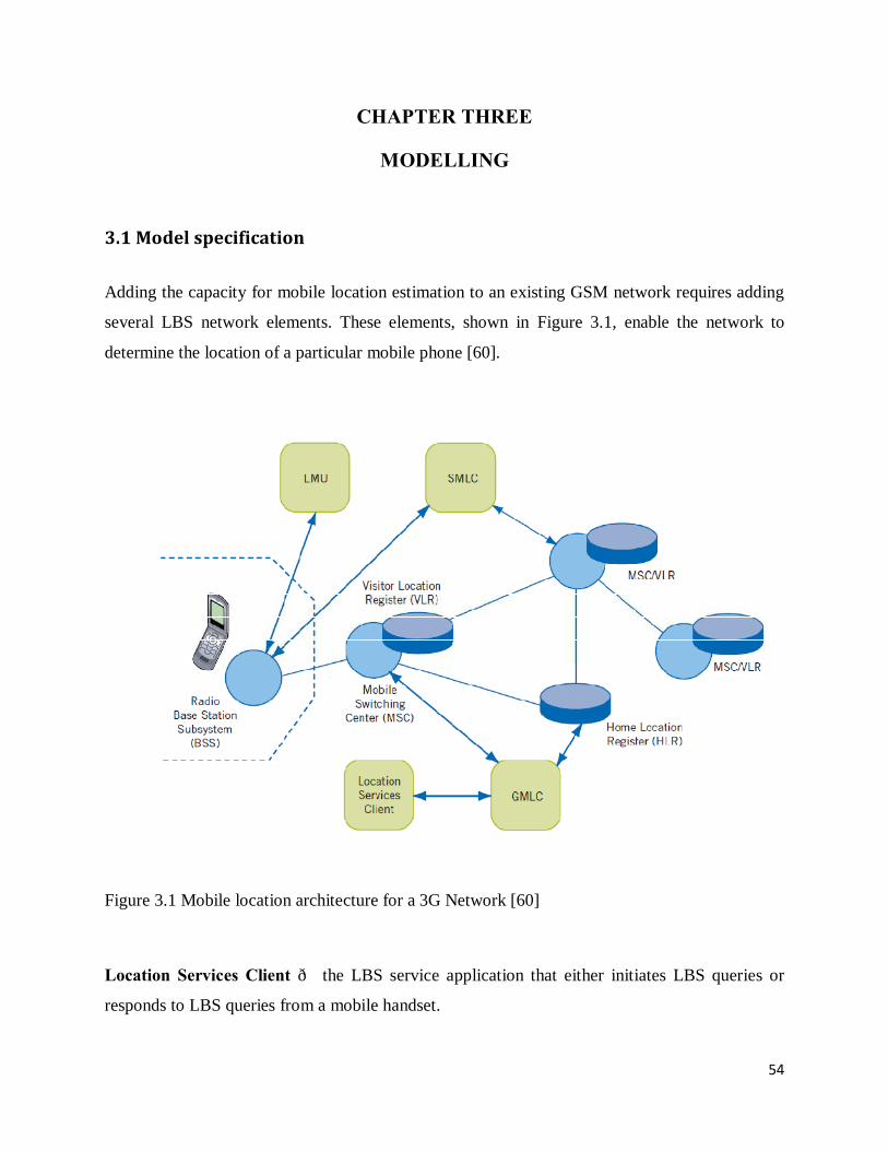
54
CHAPTER THREE
MODELLING
3.1 Model specification
Adding the capacity for mobile location estimation to an existing GSM network requires adding
several LBS network elements. These elements, shown in Figure 3.1, enable the network to
determine the location of a particular mobile phone [60].
Figure 3.1 Mobile location architecture for a 3G Network [60]
Location Services Client — the LBS service application that either initiates LBS queries or
responds to LBS queries from a mobile handset.
55
Gateway Mobile Location Center (GMLC) —the connection to the mobile network for the
client’sLBS service application. The GMLC sends requestsfor mobile handset location
information to a MobileSwitching Center (MSC) and receives the results of such requests. The
GMLC can also request routing information from the Home Location Register (HLR). (Mobile
Application Part [MAP] connections to theGMLC are via “Lh” and “Lg” interfaces.
Location Measurement Unit (LMU) — Connects with the Base Station Subsystem (BSS) of
the GSM network and takes radio measurements to support a location-based service.
Serving Mobile Location Center (SMLC) — Controls a series of LMUs in order to receive
radio interface timing measurement information. From this information, the SMLC can
determine a mobile handset’s position, plus give an indication of the accuracy of positioning
information.
Note: The SMLC and GMLC functions could be parts of a single network element
Using a coverage map of the base station distribution from MTN database, a quantitative
analysis of base station information in MTN network in Ogui region was performed. Their
position coordinates, elevations, tower heights and cell radius were noted, as well as their
relative distances from one another. The population of base stations usedconsisted of all active
base stations that form part of the 3G network. Any base station that was operational on the
network (including those that had recently gone live or are scheduled to be replaced) was
included due to the possibility that such a base station could participate in estimating the location
of a mobile phone. The model works with a minimum of 3 base stations and a maximum of 7.
The base stations used in the modeling were carefully selected to give a GDOP value that is as
low as possible.
3.2 System model design The purpose of the model design is tostudy the performance of the location estimation algorithm
in a 3G wireless network. The system model under consideration is a WCDMA 3G cellular
network. The work focuses on the case of macrocells and two-dimensional (2-D) mobile location
coordinates.
56
The simulated scenario for the WCDMA 3G cellular network consisted of a number of base
stations, up to 7, with known coordinates and which serves as landmarks, randomly distributed
within the sample space on a map drawn to scale and which serves as the simulation area. This
map is representative of a true map of the operator’s base stations distributions for a given region
in a 3G wireless network.
Simulation of the algorithm for position estimation is performed in the MATLAB software
environment having a copy of the test map.
The range difference data were created from the map by the true distances from each position of
the mobile user in the trajectory to the known Base stations. The measurement noise is assumed
to be AWGN and NLOS noise is added to the true calculated range to get the measured range
data. The measurement noise is assumed to be Gaussian distributed with zero mean.
Real data were not used in this study since it was not possible to have access to the network
facilities of any of the 3G operators in Nigeria. Besides, real data conditions the results with a
specifichardware/software implementation, and makes the result specific to a particular
environment.
The BS serving the target MS (to be located), denoted by BS#1, is called the home BS for the
MS. It is assumed that all neighboring BSs can get involved in an MS location process, provided
the signal-to-interference-plus-noise ratio (SINR) of the signal from each BS is above a certain
threshold at the MS. At all times, the MS is also assumed to be monitoring the forward pilot
channel signal levels received from the neighboring BSs and reports to the network those that
cross a given set of thresholds. The LMUs installed in the network provide the capability to
simultaneously measure the TDOA between the signal from the MS arriving at the home BS and
at any other BS.
3.2.1 Co-ordinate System Transformation
The proposed TDOA-based algorithm works with 2-D coordinates and presents results in the
same format. The X-Y co-ordinates of the Base stations of reference have to be obtained first.
The co-ordinates of Base stations are often given in the geodetic co-ordinates system (i.e. GPS
position measurement) and have to be transformed to the Local –North-East Down co-ordinate
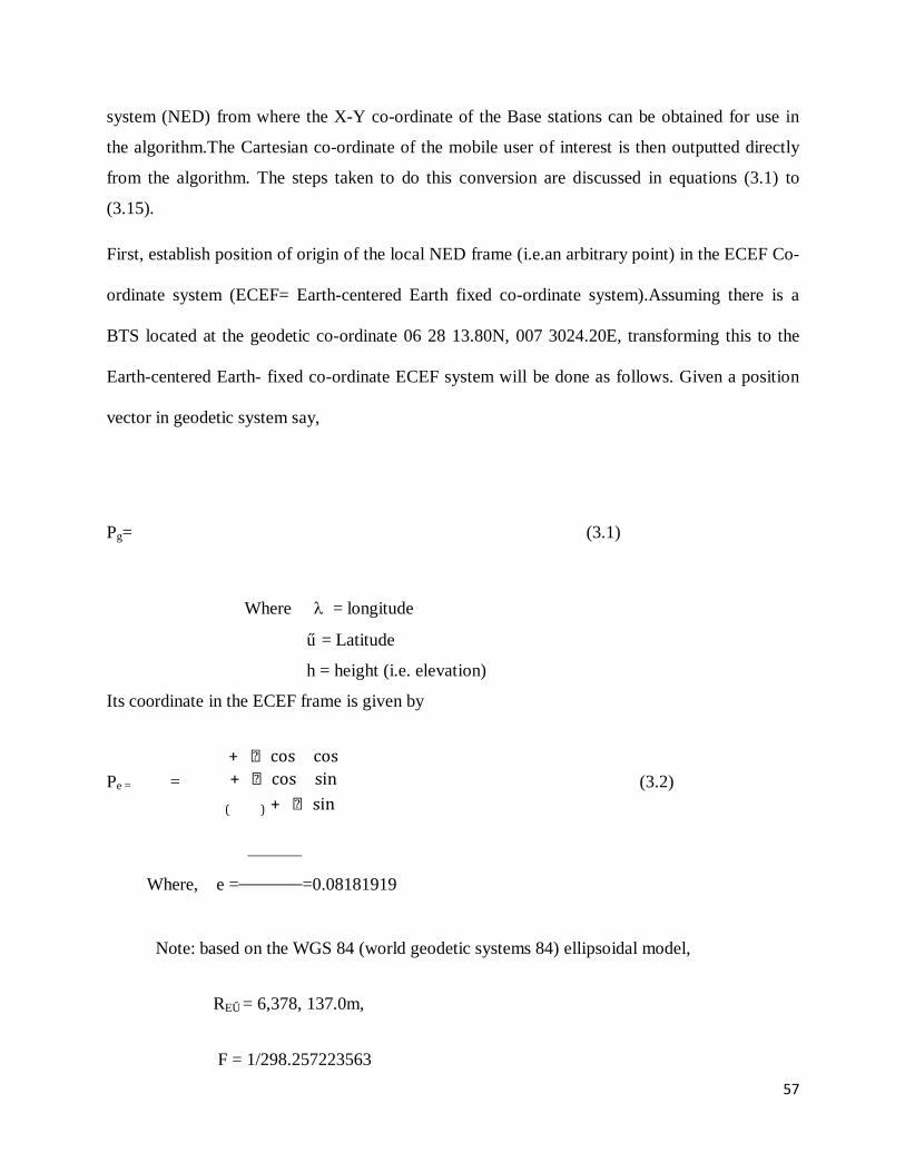
57
system (NED) from where the X-Y co-ordinate of the Base stations can be obtained for use in
the algorithm.The Cartesian co-ordinate of the mobile user of interest is then outputted directly
from the algorithm. The steps taken to do this conversion are discussed in equations (3.1) to
(3.15).
First, establish position of origin of the local NED frame (i.e.an arbitrary point) in the ECEF Co-
ordinate system (ECEF= Earth-centered Earth fixed co-ordinate system).Assuming there is a
BTS located at the geodetic co-ordinate 06 28 13.80N, 007 3024.20E, transforming this to the
Earth-centered Earth- fixed co-ordinate ECEF system will be done as follows. Given a position
vector in geodetic system say,
Pg=����
� (3.1)
Where λ = longitude
φ = Latitude
h = height (i.e. elevation)
Its coordinate in the ECEF frame is given by
Pe =�������
�= ���� + ℎ�cos � cos ���� + ℎ�cos � sin ����(����) + ℎ�sin �
� (3.2)
Where, e =� ���
� �����
���=0.08181919
Note: based on the WGS 84 (world geodetic systems 84) ellipsoidal model,
REα = 6,378, 137.0m,
F = 1/298.257223563
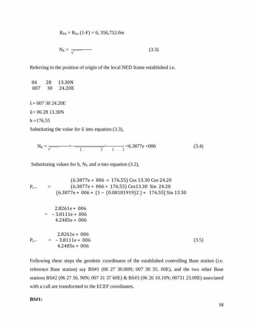
58
REb = REa (1-F) = 6, 356,752.0m
NE = ���√���������
(3.3)
Referring to the position of origin of the local NED frame established i.e.
�06 28 13.30N 007 30 24.20E�
λ= 007 30 24.20E
φ= 06 28 13.30N
h =176.55
Substituting the value for φ into equation (3.3),
NE = ���√���������
= �������.����(�.��� �����)����� (��.��)
=6.3877e +006 (3.4)
Substituting values for h, NE and λ into equation (3.2),
Pe =�������
�= � (6.3877e + 006 + 176.55) Cos 13.30 Cos 24.20(6.3877e + 006 + 176.55) Cos13.30 Sin 24.20
(6.3877e + 006 + (1 − (0.08181919)2 ) + 176.55] Sin 13.30�
= �2.8261e + 006
− 3.8111e + 006 4.2485e + 006
�
Pe = �������
�= �2.8261e + 006
− 3.8111e + 0064.2485e + 006
� (3.5)
Following these steps the geodetic coordinates of the established controlling Base station (i.e.
reference Base station) say BS#1 (06 27 30.00N; 007 30 35. 00E), and the two other Base
stations BS#2 (06 27 56. 90N; 007 31 37 60E) & BS#3 (06 26 10.10N; 00731 23.00E) associated
with a call are transformed to the ECEF coordinates.
BS#1:
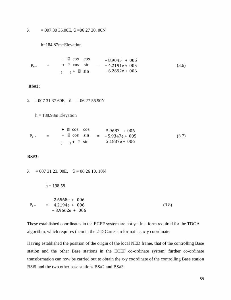
59
λ = 007 30 35.00E, φ =06 27 30. 00N
h=184.87m=Elevation
Pe =�������
�= ���� + ℎ�cos � cos ���� + ℎ�cos � sin ����(����) + ℎ�sin �
� = �− 8.9045�+ 005− 4.2191e + 005− 6.2692e + 006
� (3.6)
BS#2:
λ = 007 31 37.60E, φ = 06 27 56.90N
h = 188.98m Elevation
Pe =�������
�= ���� + ℎ�cos � cos ���� + ℎ�cos � sin ����(����) + ℎ�sin �
� = �5.9683�+ 006
− 5.9347e + 0052.1837e + 006
� (3.7)
BS#3:
λ = 007 31 23. 00E, φ = 06 26 10. 10N
h = 198.58
Pe =�������
�= �2.6568e + 0064.2194e + 006
− 3.9662e + 006� (3.8)
These established coordinates in the ECEF system are not yet in a form required for the TDOA
algorithm, which requires them in the 2-D Cartesian format i.e. x-y coordinate.
Having established the position of the origin of the local NED frame, that of the controlling Base
station and the other Base stations in the ECEF co-ordinate system; further co-ordinate
transformation can now be carried out to obtain the x-y coordinate of the controlling Base station
BS#I and the two other base stations BS#2 and BS#3.
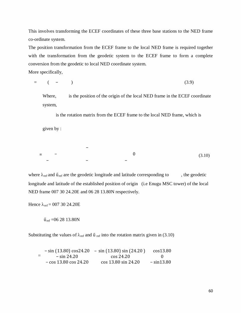
60
This involves transforming the ECEF coordinates of these three base stations to the NED frame
co-ordinate system.
The position transformation from the ECEF frame to the local NED frame is required together
with the transformation from the geodetic system to the ECEF frame to form a complete
conversion from the geodetic to local NED coordinate system.
More specifically,
�� = �� �� (��− �����) (3.9)
Where,����� is the position of the origin of the local NED frame in the ECEF coordinate
system, �� �� is the rotation matrix from the ECEF frame to the local NED frame, which is
given by :
�� �� = ��������������� − �������������� �������
− ������� ������� 0− �������������� − �������������� − �������
� (3.10)
where λref and φref are the geodetic longitude and latitude corresponding to �����, the geodetic
longitude and latitude of the established position of origin (i.e Enugu MSC tower) of the local
NED frame 007 30 24.20E and 06 28 13.80N respectively.
Hence λref = 007 30 24.20E
φref =06 28 13.80N
Substituting the values of λref and φ ref into the rotation matrix given in (3.10)
�� �� = �− sin (13.80) cos24.20 – sin (13.80) sin (24.20 ) cos13.80
− sin 24.20 cos 24.20 0− cos 13.80 cos 24.20 cos 13.80 sin 24.20 − sin13.80
�
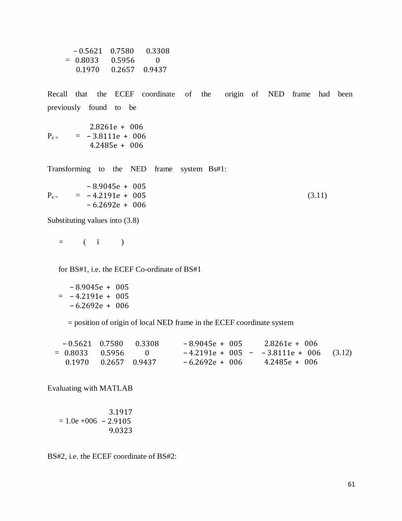
61
�� �� =�− 0.5621 0.7580 0.33080.8033 0.5956 00.1970 0.2657 0.9437
�
Recall that the ECEF coordinate of the origin of NED frame had been
previously found to be
Pe =�������
�= �2.8261e + 006
− 3.8111e + 0064.2485e + 006
�
Transforming to the NED frame system Bs#1:
Pe =�������
�= �− 8.9045e + 005− 4.2191e + 005− 6.2692e + 006
� (3.11)
Substituting values into (3.8)
�� = �� �� (�� – �����)
�� for BS#1, i.e. the ECEF Co-ordinate of BS#1
�� = �− 8.9045e + 005− 4.2191e + 005− 6.2692e + 006
�
����� = position of origin of local NED frame in the ECEF coordinate system
��=�− 0.5621 0.7580 0.33080.8033 0.5956 00.1970 0.2657 0.9437
� ��− 8.9045e + 005− 4.2191e + 005− 6.2692e + 006
� − �2.8261e + 006
− 3.8111e + 0064.2485e + 006
��� (3.12)
Evaluating with MATLAB
�� = 1.0e +006�3.1917
− 2.9105 9.0323
�
BS#2, i.e. the ECEF coordinate of BS#2:
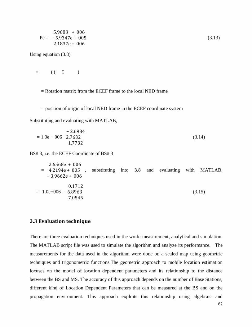
62
Pe =�5.9683�+ 006
− 5.9347e + 0052.1837e + 006
� (3.13)
Using equation (3.8)
�� = �� �� ( (�� – �����)
�� �� = Rotation matrix from the ECEF frame to the local NED frame
�����= position of origin of local NED frame in the ECEF coordinate system
Substituting and evaluating with MATLAB,
�� = 1.0e + 006�− 2.6984
2.7632 1.7732
� (3.14)
BS# 3, i.e. the ECEF Coordinate of BS# 3
�� =� 2.6568e + 0064.2194e + 005
− 3.9662e + 006�, substituting into 3.8 and evaluating with MATLAB,
�� = 1.0e+006�0.1712
− 6.8963 7.0545
� (3.15)
3.3 Evaluation technique
There are three evaluation techniques used in the work: measurement, analytical and simulation.
The MATLAB script file was used to simulate the algorithm and analyze its performance. The
measurements for the data used in the algorithm were done on a scaled map using geometric
techniques and trigonometric functions.The geometric approach to mobile location estimation
focuses on the model of location dependent parameters and its relationship to the distance
between the BS and MS. The accuracy of this approach depends on the number of Base Stations,
different kind of Location Dependent Parameters that can be measured at the BS and on the
propagation environment. This approach exploits this relationship using algebraic and
63
trigonometric calculations to estimate the location of the MS.Circular trilateration (CT) is one of
the most prominent techniques under this approach.
To evaluate the accuracy of the results obtained, the calculated 2-D location coordinates of the
mobile station were compared to observations of their actual location coordinates provided on
the real map.
3.4 Performance metrics
The accuracy of the location estimates obtained during mobile location could be impaired by
some factors. In [61] a study was done on the accuracy with which the location of base stations
in a network are known, as inaccuracies in the given locations of these base stations can
negatively affect the ability of many methods and algorithms to provide accurate Mobile station
location estimates. The identified factors, apart from negatively impacting accuracy, also
increase the cost of estimating the location of the mobile device. These factors include non-line-
of sight and multi-path propagation of radio waves, the base station density (or lack of it) and
accuracy of base station locations, optimizations for network capacity, and the unsynchronized
nature of UMTS type networks.
The following metrics are used to compare the overall performance of a geolocation technique:
1. Location accuracy of a geolocation method is defined to be the distance between the
estimated location and the true location of the mobile station. Accuracy is expressed in
meters.
There are a number of performance metrics for location accuracy in the literature:
i. Root Mean Square Error (RMSE) and the Mean Squared Error (MSE),
The performance metrics used in this research to analyze location accuracy for the algorithm is
the distance error and RMSE Root Mean Square Error (RMSE). Distance error is defined as
� = �(���� − �����)� + (���� − �����)� (3.16)
64
Where (Xest,Yest) is the estimated coordinates, and (Xtrue, Ytrue) is the true location coordinates of
the mobile station. Therefore define RMSE can be defined as
�� �� = �∑ ��
�
�� (3.17)
Where �� represent the errors and n denotes the number of location estimates made in a set. The
set may contain either all the attempted location measurements or only the successful ones. If
only the successful location are used, the ratio of successful location measurements out of all
attempted location measurements is called the reliability of the system
The RMSE is the most applicable location accuracy performance metric in the literature; it is the
most used and a simple metric. This is a lower better (LB) metric. Mathematically RMSE is also
defined as
�� �� = √� �� (3.18)
Where � �� = ∑ ���
�� (3.19)
ii. Geometric Dilution 0f Precision (GDOP)
Geometric dilution of precision (GDOP) can be applied as a criterion for choosing the right
geometric configuration of the measurement units such as base stations (BSs) and mobile station
(MS).
For both TOA and TDOA schemes, the accuracy of range-based Position Location systems
depends to a large extent on the physical geometry of the link between the base stations and the
source to be located. One measure that quantifies the accuracy based on this geometric
configuration is called the geometric dilution of precision (GDOP). The GDOP can be used as a
criterion for selecting a set of base stations from a large set whose measurements produce
minimum Position location estimation error or for designing base station locations within new
systems. It is desired that GDOP value be always a minimum. Assuming a measurement
accuracy of 10m and GDOP value of 5, our positioning accuracy becomes 50 m. If the
GDOP value is close to unity, then our positioning accuracy gets close to our measurement
accuracy
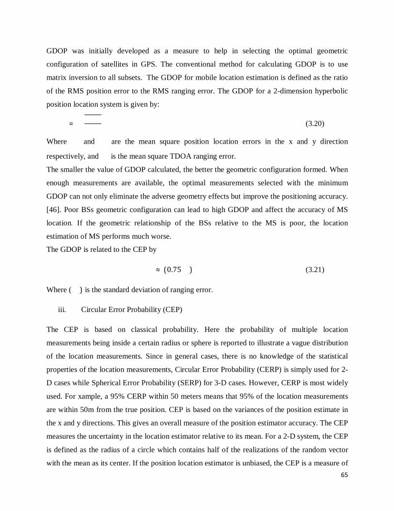
65
GDOP was initially developed as a measure to help in selecting the optimal geometric
configuration of satellites in GPS. The conventional method for calculating GDOP is to use
matrix inversion to all subsets. The GDOP for mobile location estimation is defined as the ratio
of the RMS position error to the RMS ranging error. The GDOP for a 2-dimension hyperbolic
position location system is given by:
���� = � ������
�
��� (3.20)
Where ��� and ��
� are the mean square position location errors in the x and y direction
respectively, and ��� is the mean square TDOA ranging error.
The smaller the value of GDOP calculated, the better the geometric configuration formed. When
enough measurements are available, the optimal measurements selected with the minimum
GDOP can not only eliminate the adverse geometry effects but improve the positioning accuracy.
[46]. Poor BSs geometric configuration can lead to high GDOP and affect the accuracy of MS
location. If the geometric relationship of the BSs relative to the MS is poor, the location
estimation of MS performs much worse.
The GDOP is related to the CEP by
��� ≈ (0.75��)���� (3.21)
Where (��) is the standard deviation of ranging error.
iii. Circular Error Probability (CEP)
The CEP is based on classical probability. Here the probability of multiple location
measurements being inside a certain radius or sphere is reported to illustrate a vague distribution
of the location measurements. Since in general cases, there is no knowledge of the statistical
properties of the location measurements, Circular Error Probability (CERP) is simply used for 2-
D cases while Spherical Error Probability (SERP) for 3-D cases. However, CERP is most widely
used. For xample, a 95% CERP within 50 meters means that 95% of the location measurements
are within 50m from the true position. CEP is based on the variances of the position estimate in
the x and y directions. This gives an overall measure of the position estimator accuracy. The CEP
measures the uncertainty in the location estimator relative to its mean. For a 2-D system, the CEP
is defined as the radius of a circle which contains half of the realizations of the random vector
with the mean as its center. If the position location estimator is unbiased, the CEP is a measure of
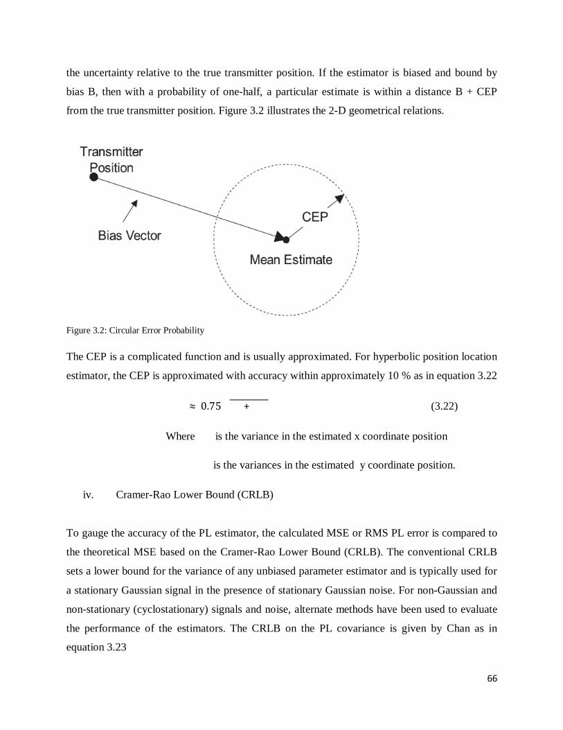
66
the uncertainty relative to the true transmitter position. If the estimator is biased and bound by
bias B, then with a probability of one-half, a particular estimate is within a distance B + CEP
from the true transmitter position. Figure 3.2 illustrates the 2-D geometrical relations.
Figure 3.2: Circular Error Probability
The CEP is a complicated function and is usually approximated. For hyperbolic position location
estimator, the CEP is approximated with accuracy within approximately 10 % as in equation 3.22
��� ≈ 0.75���� + ��
� (3.22)
Where ��� is the variance in the estimated x coordinate position
��� is the variances in the estimated y coordinate position.
iv. Cramer-Rao Lower Bound (CRLB)
To gauge the accuracy of the PL estimator, the calculated MSE or RMS PL error is compared to
the theoretical MSE based on the Cramer-Rao Lower Bound (CRLB). The conventional CRLB
sets a lower bound for the variance of any unbiased parameter estimator and is typically used for
a stationary Gaussian signal in the presence of stationary Gaussian noise. For non-Gaussian and
non-stationary (cyclostationary) signals and noise, alternate methods have been used to evaluate
the performance of the estimators. The CRLB on the PL covariance is given by Chan as in
equation 3.23
67
���� = ��(��������)�� (3.23)
�� = (�, �, ��) , which correspond to the actual coordinates of the source and the range of the
first base station to the source, and matrix Q is the TDOA covariance matrix. The sum of the
diagonal elements of ɸ defines the theoretical lower bound on the MSE of the Position location
estimator. Matrix Q may not be known in practice; however if the noise power spectral densities
are similar at the receivers, it can be replaced by a theoretical TDOA covariance matrix with
diagonal elements of ��� and 0.5��
� for all other elements, where ��� is the variance of the TDOA
estimate.
2. Computational Efficiency: This metric defines the number of Floating Point Operations
(FLOPS) which the algorithm uses as it runs. Higher FLOPS indicate the algorithm is less
computationally efficient.
3.5 Parameters considered in the work: System parameters are characteristics of the system that may affect the overall performance of
the system, which in this case is the algorithm proposed in this work.
These parameters include:
1. Mobility of mobile station under investigation,
2. Number of mobile stations considered,
3. Number of base stations used,
4. TDOA estimation error,
5. Coverage area of the BTS,
6. Environment Type,
7. Cell size
Some other parameters/factors were varied in order to study the performance of the algorithm
when applied in a 3G network algorithm. These are described below.
1. Mobility of Stations: In order to locate mobile stations, both stationary and mobile routes are
considered. But for this work, only stationary cases were considered and simulated. However,
the positions of the base stations were varied at different instances to analyze the performance of
68
the algorithm under those instances. The stationary cases represent scenarios of a cell phone user
requiring an emergency aid from a fixed position.
2. Number of Base Stations: The TDOA method requires at least three base stations in order to
get a location estimate for a mobile station. Four or more base stations are expected to increase
the location accuracy. At least three base stations are assumed to be present in the area where the
algorithm is to be applied.
3. Range difference: this refers to the absolute difference between the distances from the BTSs
positions to the position of the MS to be located
4. TDOA Estimation Error: This factor is also known as TDOA measurement noise.
It defines the errors that would be present in the TDOA measurements themselves. These
measurements are done in the LMUs found in the network.
The values for this factor are: 50 nanosecond (ns), 100 ns, 200ns, and 400 ns. 4. Environment type: The required accuracy of mobile user's location depends on the
environment in which geolocation technique is applied. The mobile station's radio signal reaches
the base stations via multiple paths, bouncing-off various man-made and natural obstacles. This
factor, called multipath, has a direct effect on location accuracy. It is likely that the probability of
observing multiple base station signals is higher in bad urban environments than in rural areas.
Since environmenthas a significant effect on the performance metric chosen, this study takes into
account this dependence on the environment. The environment type chosen for this study is the
urban area. This refers to sparsely inhibited areas, fields and forests.
3.6 Hyperbolic Equation model and Solution Algorithms Once a measure of the TDOAs has been obtained, they are converted into range difference
measurements and these measurements can be converted into nonlinear hyperbolic equations.
As these equations are non-linear, solving them is not a trivial operation. Several algorithms have
been proposed for this purpose, with each having different complexities and degrees of accuracy.

69
First discuss the mathematical model that is used by these algorithms in arriving at the
hyperbolic equations will be discussed. This is then followed by a detailed description
ofcoordinate systems transformation method, performance metrics for position location
algorithms, and the algorithm proposed in this work for solving the hyperbolic equations.
A general model for the two dimensional (2-D) mobile position estimates for an MS using M
number of Base Stations is developed. All TDOA measurements will be done in reference to the
first Base station, which is assumed to be the Base station controlling the call and first to receive
the transmitted signal from the MS. This will be called the reference Base station.
Let the index i = 2, 3…, M, represent the number of Base stations, let (x, y) be 2-D location of
the MS and (Xi; Yi) be the known location of the ith Base station receiving the signal from the
MS.
The range distance between the MS and the ith receiver is given as:
�� = �(��− �)� + (��− �)�
= ���� + ��
� − 2��� − 2��� + �� + �� (3.24)
The range difference between the other Base stations receiving signal from the MS with respect
to the reference Base station will be obtained by transforming TDOA values into range
difference measurements using the equation:
��, 1 = �∗ ��, 1 = ��− �� = �(��− �)� + (��− �)� − �(�� − �)� + (�� − �)� (3.25)
This is a set of nonlinear hyperbolic equations whose solution gives the 2-D coordinates of the
MS’s location.
Solving this nonlinear equation is difficult as has been stated earlier. Consequently, linearizing
this equation is commonly performed and one way to do that is through the use of Taylor-series
expansion.
A commonly used alternative method to the Taylor-series expansion method is to first transform
the set of nonlinear equations in (3.25) into another set of equations.
Rearranging the form of (3.25) into:
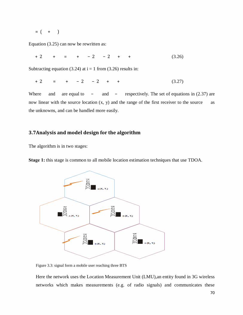
70
��� = (��+ ��)�
Equation (3.25) can now be rewritten as:
��� + 2���� + ��
� = ��� + ��
� − 2��� − 2��� + �� + �� (3.26)
Subtracting equation (3.24) at i = 1 from (3.26) results in:
��� + 2���� = ��
� + ��� − 2��� − 2��� + �� + �� (3.27)
Where �� and �� are equal to ��− �� and ��− �� respectively. The set of equations in (2.37) are
now linear with the source location (x, y) and the range of the first receiver to the source �� as
the unknowns, and can be handled more easily.
3.7Analysis and model design for the algorithm The algorithm is in two stages:
Stage 1: this stage is common to all mobile location estimation techniques that use TDOA.
Figure 3.3: signal form a mobile user reaching three BTS
Here the network uses the Location Measurement Unit (LMU),an entity found in 3G wireless
networks which makes measurements (e.g. of radio signals) and communicates these
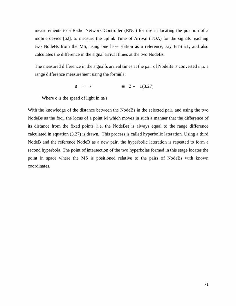
71
measurements to a Radio Network Controller (RNC) for use in locating the position of a
mobile device [62], to measure the uplink Time of Arrival (TOA) for the signals reaching
two NodeBs from the MS, using one base station as a reference, say BTS #1; and also
calculates the difference in the signal arrival times at the two NodeBs.
The measured difference in the signal’s arrival times at the pair of NodeBs is converted into a
range difference measurement using the formula:
∆� = �∗ ��������� ��� ≅ �2 − �1(3.27)
Where c is the speed of light in m/s
With the knowledge of the distance between the NodeBs in the selected pair, and using the two
NodeBs as the foci, the locus of a point M which moves in such a manner that the difference of
its distance from the fixed points (i.e. the NodeBs) is always equal to the range difference
calculated in equation (3.27) is drawn. This process is called hyperbolic lateration. Using a third
NodeB and the reference NodeB as a new pair, the hyperbolic lateration is repeated to form a
second hyperbola. The point of intersection of the two hyperbolas formed in this stage locates the
point in space where the MS is positioned relative to the pairs of NodeBs with known
coordinates.
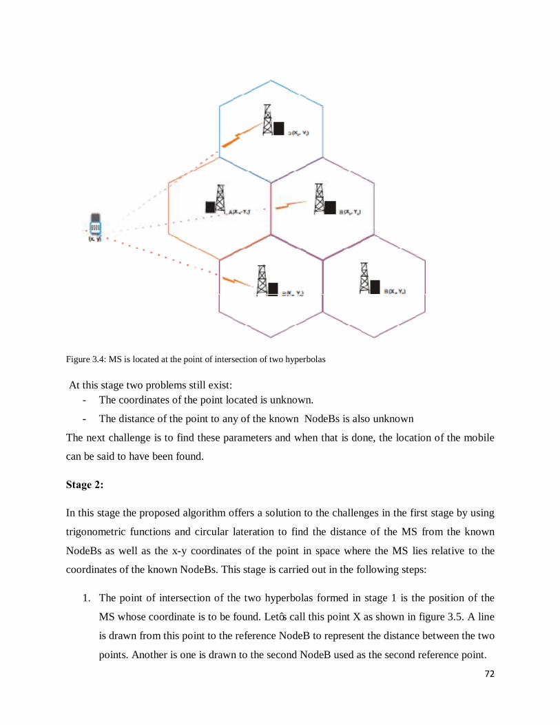
72
Figure 3.4: MS is located at the point of intersection of two hyperbolas
At this stage two problems still exist: - The coordinates of the point located is unknown.
- The distance of the point to any of the known NodeBs is also unknown
The next challenge is to find these parameters and when that is done, the location of the mobile
can be said to have been found.
Stage 2:
In this stage the proposed algorithm offers a solution to the challenges in the first stage by using
trigonometric functions and circular lateration to find the distance of the MS from the known
NodeBs as well as the x-y coordinates of the point in space where the MS lies relative to the
coordinates of the known NodeBs. This stage is carried out in the following steps:
1. The point of intersection of the two hyperbolas formed in stage 1 is the position of the
MS whose coordinate is to be found. Let’s call this point X as shown in figure 3.5. A line
is drawn from this point to the reference NodeB to represent the distance between the two
points. Another is one is drawn to the second NodeB used as the second reference point.
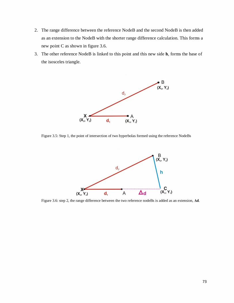
73
2. The range difference between the reference NodeB and the second NodeB is then added
as an extension to the NodeB with the shorter range difference calculation. This forms a
new point C as shown in figure 3.6.
3. The other reference NodeB is linked to this point and this new side h, forms the base of
the isosceles triangle.
Figure 3.5: Step 1, the point of intersection of two hyperbolas formed using the reference NodeBs
Figure 3.6: step 2, the range difference between the two reference nodeBs is added as an extension, Δd.
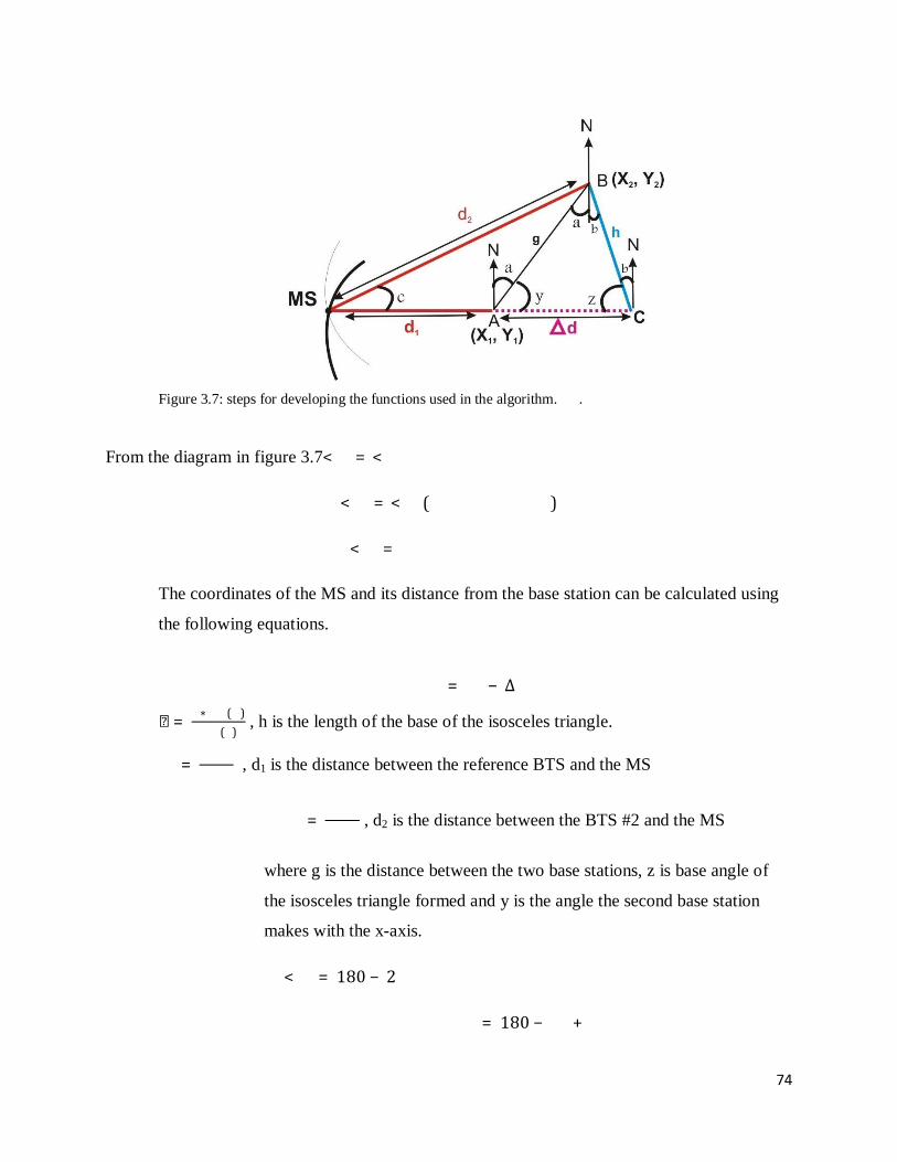
74
Figure 3.7: steps for developing the functions used in the algorithm. .
From the diagram in figure 3.7< � = < ������������
< � = < � (��������������)
< � = �������������� �
The coordinates of the MS and its distance from the base station can be calculated using
the following equations.
�� = �� − ∆�
ℎ = �∗��� (�)��� (�)
, h is the length of the base of the isosceles triangle.
�� = ���������
, d1 is the distance between the reference BTS and the MS
�� = ���������
, d2 is the distance between the BTS #2 and the MS
where g is the distance between the two base stations, z is base angle of
the isosceles triangle formed and y is the angle the second base station
makes with the x-axis.
< � = 180 − 2�
� = 180 − �� + ��

75
But � = 180 − �
� = 180 − �� + 180 − ��
= 180 − 180 − � + �
∴ � = � − �
�� = ��∗����������
, di is the distance between the BTS #i and the MS
Where �� is the distance between the first and ith base station, ��is the
angle the BTS #i makes with the x-axis and
�� = 180 − 2 ∗ ��
�� = ��− ��
Z3 is the base angle of the second isosceles angle.
�� = ���� − ��� + ��� − ���
��� = (�� − �)� + (�� − �)� (3.28)
��� = ��
� − 2���+ �� + ��� − 2��� + ��
�� = �(�� − �)� + (�� − �)�
��� = (�� − �)� + (�� − �)� (3.29)
��� = ��
� − 2���+ �� + ��� − 2��� + ��
�� = �(��− �)� + (��− �)� (3.30)
��� = (��− �)� + (��− �)� (3.31)
��� = ��
� − 2���+ �� + ��� − 2��� + ��
X1 and Y1 are the known coordinates of the first base station
X2 and Y2 are the known coordinates of the second base station
76
Xi and Yi are the known coordinates of the ith base station
X and Y are the Unknown Coordinates of the MS
d1 = distance of the first base station from the MS
d2 = distance of the MS from second base station
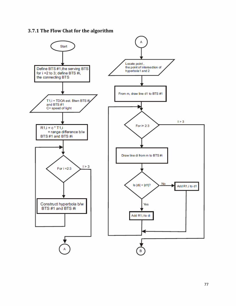
77
3.7.1 The Flow Chat for the algorithm
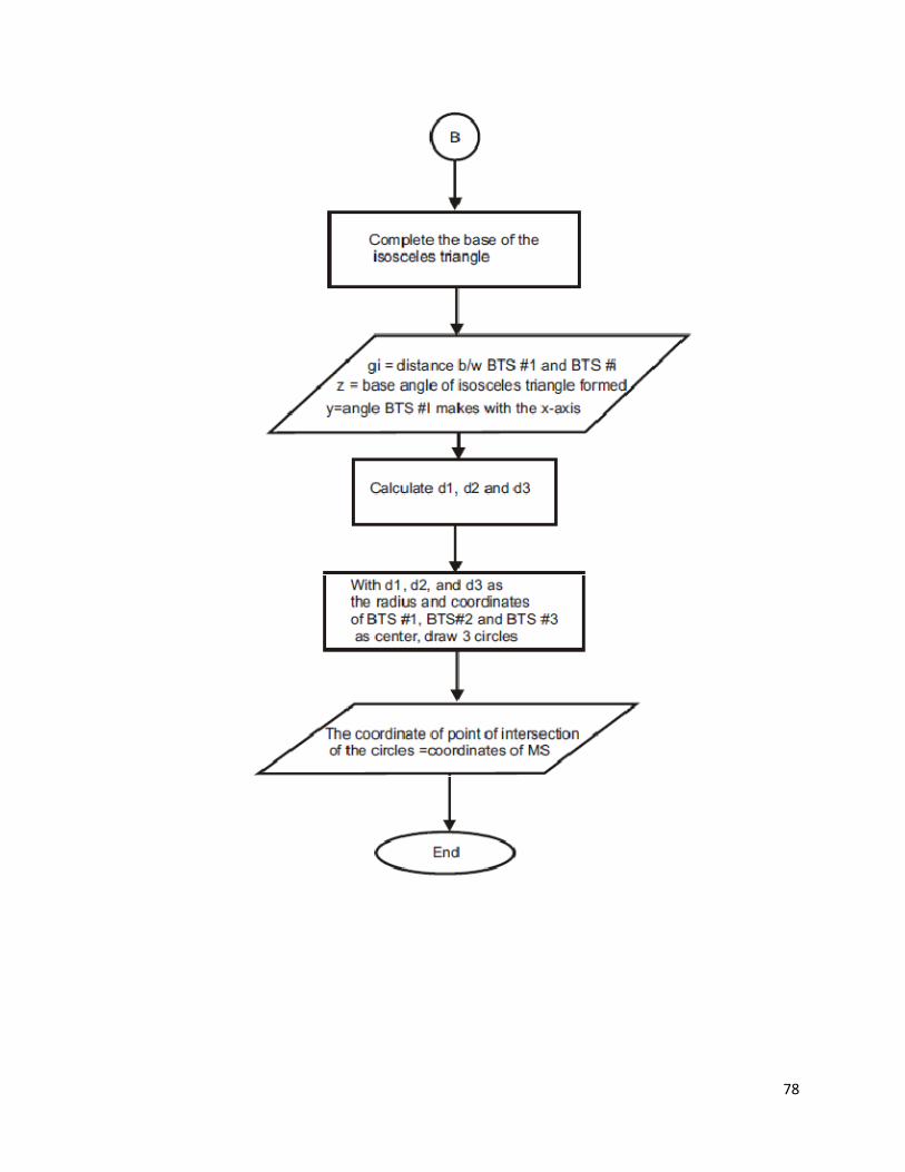
78
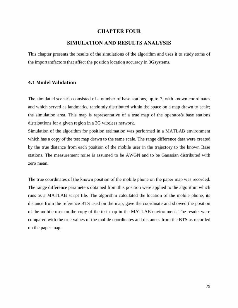
79
CHAPTER FOUR
SIMULATION AND RESULTS ANALYSIS
This chapter presents the results of the simulations of the algorithm and uses it to study some of
the importantfactors that affect the position location accuracy in 3Gsystems.
4.1 Model Validation
The simulated scenario consisted of a number of base stations, up to 7, with known coordinates
and which served as landmarks, randomly distributed within the space on a map drawn to scale;
the simulation area. This map is representative of a true map of the operator’s base stations
distributions for a given region in a 3G wireless network.
Simulation of the algorithm for position estimation was performed in a MATLAB environment
which has a copy of the test map drawn to the same scale. The range difference data were created
by the true distance from each position of the mobile user in the trajectory to the known Base
stations. The measurement noise is assumed to be AWGN and to be Gaussian distributed with
zero mean.
The true coordinates of the known position of the mobile phone on the paper map was recorded.
The range difference parameters obtained from this position were applied to the algorithm which
runs as a MATLAB script file. The algorithm calculated the location of the mobile phone, its
distance from the reference BTS used on the map, gave the coordinate and showed the position
of the mobile user on the copy of the test map in the MATLAB environment. The results were
compared with the true values of the mobile coordinates and distances from the BTS as recorded
on the paper map.
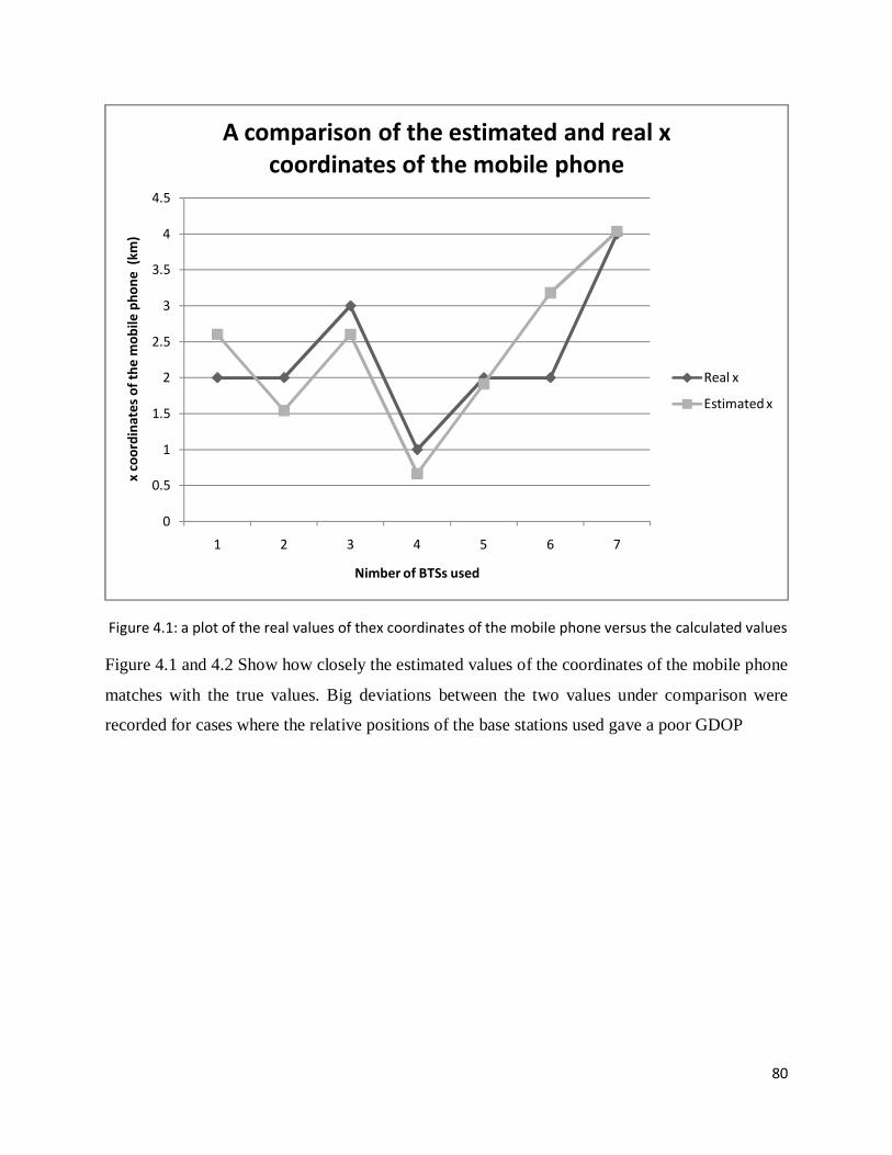
80
Figure 4.1: a plot of the real values of thex coordinates of the mobile phone versus the calculated values
Figure 4.1 and 4.2 Show how closely the estimated values of the coordinates of the mobile phone
matches with the true values. Big deviations between the two values under comparison were
recorded for cases where the relative positions of the base stations used gave a poor GDOP
0
0.5
1
1.5
2
2.5
3
3.5
4
4.5
1 2 3 4 5 6 7
x co
ordi
nate
s of t
he m
obile
pho
ne (
km)
Nimber of BTSs used
A comparison of the estimated and real x coordinates of the mobile phone
Real x
Estimated x
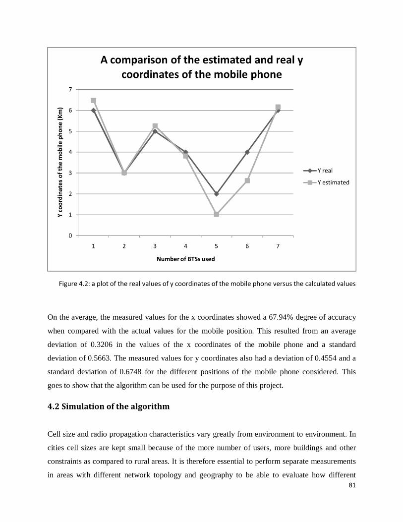
81
Figure 4.2: a plot of the real values of y coordinates of the mobile phone versus the calculated values
On the average, the measured values for the x coordinates showed a 67.94% degree of accuracy
when compared with the actual values for the mobile position. This resulted from an average
deviation of 0.3206 in the values of the x coordinates of the mobile phone and a standard
deviation of 0.5663. The measured values for y coordinates also had a deviation of 0.4554 and a
standard deviation of 0.6748 for the different positions of the mobile phone considered. This
goes to show that the algorithm can be used for the purpose of this project.
4.2 Simulation of the algorithm
Cell size and radio propagation characteristics vary greatly from environment to environment. In
cities cell sizes are kept small because of the more number of users, more buildings and other
constraints as compared to rural areas. It is therefore essential to perform separate measurements
in areas with different network topology and geography to be able to evaluate how different
0
1
2
3
4
5
6
7
1 2 3 4 5 6 7
Y co
ordi
nate
s of t
he m
obile
pho
ne (K
m)
Number of BTSs used
A comparison of the estimated and real y coordinates of the mobile phone
Y real
Y estimated
82
propagation properties are influencing the accuracy of the location method and algorithm used.
Two different measurement scenarios, the urban and rural areas are often investigated. In this
work, the simulation of the algorithm and analysis of the results obtained was done using the
MATLAB and Microsoft Excel application respectively, and assumed the urban scenario.
Urban areas measurements are usually performed for an area consisting of both micro GSM900
and GSM19800 cells. Microcells are average sized radio cells with diameters of one to two
kilometers. These types of cells give large capacity for a small area.
In section 4.3the degree of disparity in the actual and estimated values of the coordinates of the
mobile device to be located is studied while varying the positions of a set of three BTS in the 3G
cellular environments. The discussion that follows looks at the effect of increasing the number of
BTSs on the RMSE in the mobile position estimate and the dependence of error in MS distance
measurement on the number of BTS used in the calculation.The effect of Geometric Dilution of
Precision (GDOP) on the performance of the position location algorithm is studied in section 4.5.
With the help of the results obtained, optimal positions for the set of BTSs used in the calculation
will be suggested.
Figure 4.3: Sample MS Location diagram from MATLAB using the Algorithm
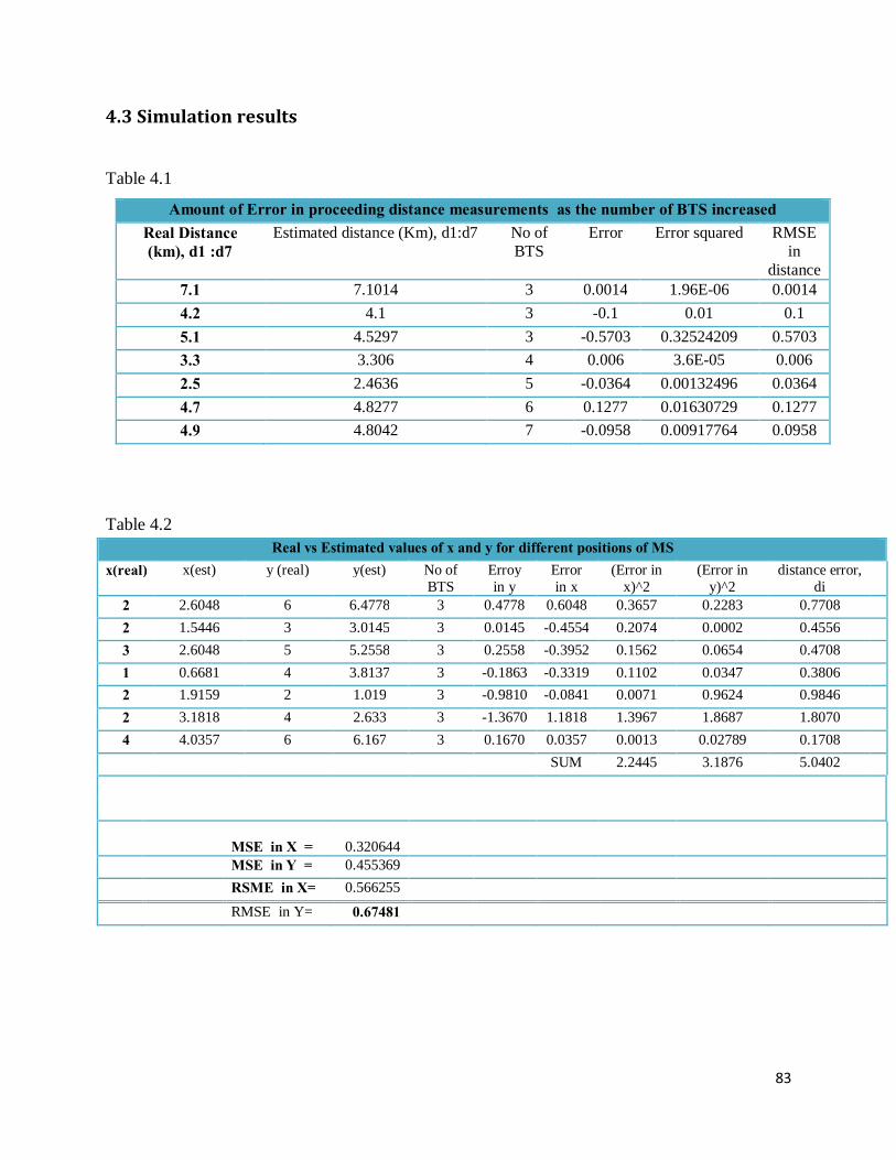
83
4.3 Simulation results
Table 4.1
Amount of Error in proceeding distance measurements as the number of BTS increased Real Distance (km), d1 :d7
Estimated distance (Km), d1:d7 No of BTS
Error Error squared RMSE in
distance 7.1 7.1014 3 0.0014 1.96E-06 0.0014 4.2 4.1 3 -0.1 0.01 0.1 5.1 4.5297 3 -0.5703 0.32524209 0.5703 3.3 3.306 4 0.006 3.6E-05 0.006 2.5 2.4636 5 -0.0364 0.00132496 0.0364 4.7 4.8277 6 0.1277 0.01630729 0.1277 4.9 4.8042 7 -0.0958 0.00917764 0.0958
Table 4.2
Real vs Estimated values of x and y for different positions of MS x(real) x(est) y (real) y(est) No of
BTS Erroy in y
Error in x
(Error in x)^2
(Error in y)^2
distance error, di
2 2.6048 6 6.4778 3 0.4778 0.6048 0.3657 0.2283 0.7708 2 1.5446 3 3.0145 3 0.0145 -0.4554 0.2074 0.0002 0.4556 3 2.6048 5 5.2558 3 0.2558 -0.3952 0.1562 0.0654 0.4708 1 0.6681 4 3.8137 3 -0.1863 -0.3319 0.1102 0.0347 0.3806 2 1.9159 2 1.019 3 -0.9810 -0.0841 0.0071 0.9624 0.9846 2 3.1818 4 2.633 3 -1.3670 1.1818 1.3967 1.8687 1.8070 4 4.0357 6 6.167 3 0.1670 0.0357 0.0013 0.02789 0.1708 SUM 2.2445 3.1876 5.0402
MSE in X =
0.320644
MSE in Y = 0.455369 RSME in X= 0.566255 RMSE in Y= 0.67481
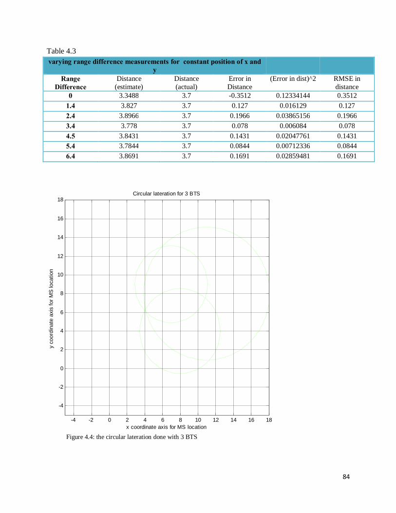
84
Table 4.3 varying range difference measurements for constant position of x and
y
Range Difference
Distance (estimate)
Distance (actual)
Error in Distance
(Error in dist)^2 RMSE in distance
0 3.3488 3.7 -0.3512 0.12334144 0.3512 1.4 3.827 3.7 0.127 0.016129 0.127 2.4 3.8966 3.7 0.1966 0.03865156 0.1966 3.4 3.778 3.7 0.078 0.006084 0.078 4.5 3.8431 3.7 0.1431 0.02047761 0.1431 5.4 3.7844 3.7 0.0844 0.00712336 0.0844 6.4 3.8691 3.7 0.1691 0.02859481 0.1691
Figure 4.4: the circular lateration done with 3 BTS
x coordinate axis for MS location
y co
ordi
nate
axi
s fo
r MS
loca
tion
Circular lateration for 3 BTS
-4 -2 0 2 4 6 8 10 12 14 16 18
-4
-2
0
2
4
6
8
10
12
14
16
18
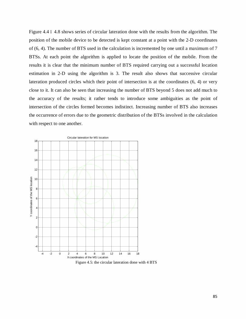
85
Figure 4.4 – 4.8 shows series of circular lateration done with the results from the algorithm. The
position of the mobile device to be detected is kept constant at a point with the 2-D coordinates
of (6, 4). The number of BTS used in the calculation is incremented by one until a maximum of 7
BTSs. At each point the algorithm is applied to locate the position of the mobile. From the
results it is clear that the minimum number of BTS required carrying out a successful location
estimation in 2-D using the algorithm is 3. The result also shows that successive circular
lateration produced circles which their point of intersection is at the coordinates (6, 4) or very
close to it. It can also be seen that increasing the number of BTS beyond 5 does not add much to
the accuracy of the results; it rather tends to introduce some ambiguities as the point of
intersection of the circles formed becomes indistinct. Increasing number of BTS also increases
the occurrence of errors due to the geometric distribution of the BTSs involved in the calculation
with respect to one another.
Figure 4.5: the circular lateration done with 4 BTS
X coordinates of the MS Location
Y co
ordi
nate
s of
the
MS
loca
tion
Circular lateration for MS location
-4 -2 0 2 4 6 8 10 12 14 16 18
-4
-2
0
2
4
6
8
10
12
14
16
18
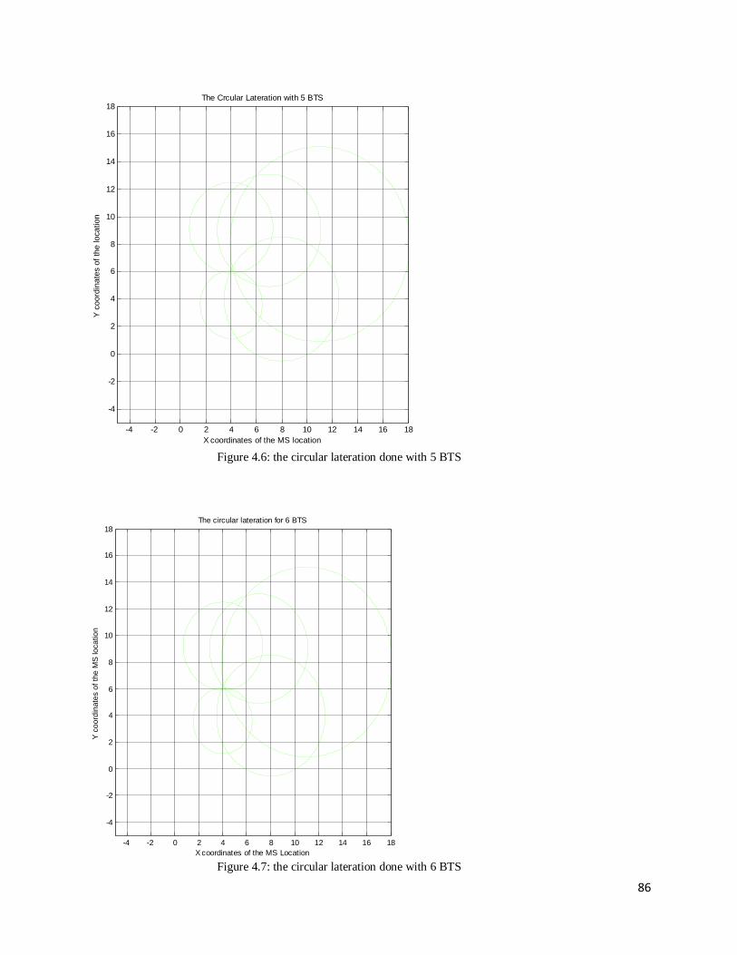
86
Figure 4.6: the circular lateration done with 5 BTS
Figure 4.7: the circular lateration done with 6 BTS
X coordinates of the MS location
Y co
ordi
nate
s of
the
loca
tion
The Crcular Lateration with 5 BTS
-4 -2 0 2 4 6 8 10 12 14 16 18
-4
-2
0
2
4
6
8
10
12
14
16
18
X coordinates of the MS Location
Y co
ordi
nate
s of
the
MS
loca
tion
The circular lateration for 6 BTS
-4 -2 0 2 4 6 8 10 12 14 16 18
-4
-2
0
2
4
6
8
10
12
14
16
18

87
Figure 4.8: the circular lateration done with 7 BTS
X coordinates of the MS location
Y co
ordi
nate
s of
MS
loca
tion
The circular lateration with 7 BTS
-4 -2 0 2 4 6 8 10 12 14 16 18
-4
-2
0
2
4
6
8
10
12
14
16
18
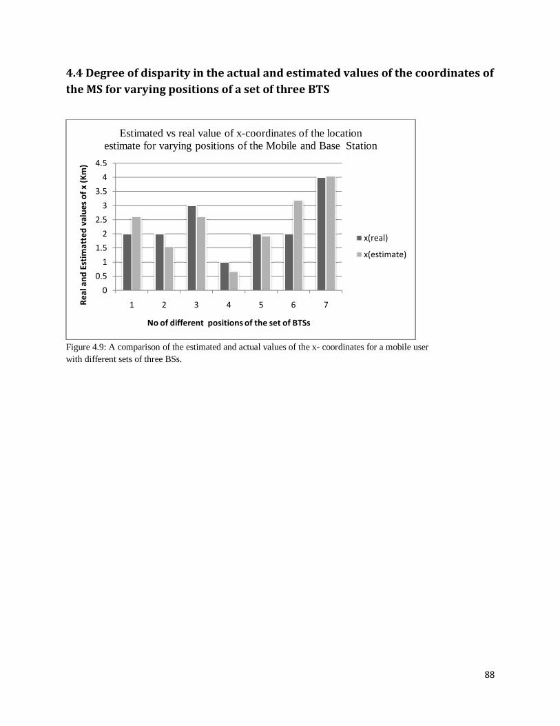
88
4.4 Degree of disparity in the actual and estimated values of the coordinates of the MS for varying positions of a set of three BTS
Figure 4.9: A comparison of the estimated and actual values of the x- coordinates for a mobile user with different sets of three BSs.
00.5
11.5
22.5
33.5
44.5
1 2 3 4 5 6 7Real
and
Est
imat
ted
valu
es o
f x (K
m)
No of different positions of the set of BTSs
Estimated vs real value of x-coordinates of the location estimate for varying positions of the Mobile and Base Station
x(real)
x(estimate)
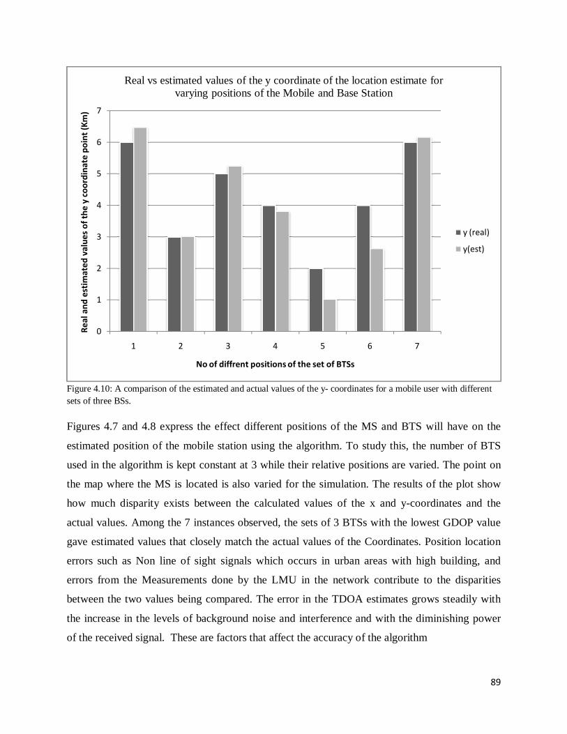
89
Figure 4.10: A comparison of the estimated and actual values of the y- coordinates for a mobile user with different sets of three BSs. Figures 4.7 and 4.8 express the effect different positions of the MS and BTS will have on the
estimated position of the mobile station using the algorithm. To study this, the number of BTS
used in the algorithm is kept constant at 3 while their relative positions are varied. The point on
the map where the MS is located is also varied for the simulation. The results of the plot show
how much disparity exists between the calculated values of the x and y-coordinates and the
actual values. Among the 7 instances observed, the sets of 3 BTSs with the lowest GDOP value
gave estimated values that closely match the actual values of the Coordinates. Position location
errors such as Non line of sight signals which occurs in urban areas with high building, and
errors from the Measurements done by the LMU in the network contribute to the disparities
between the two values being compared. The error in the TDOA estimates grows steadily with
the increase in the levels of background noise and interference and with the diminishing power
of the received signal. These are factors that affect the accuracy of the algorithm
0
1
2
3
4
5
6
7
1 2 3 4 5 6 7
Real
and
est
imat
ed v
alue
s of t
he y
coor
dina
te p
oint
(Km
)
No of diffrent positions of the set of BTSs
Real vs estimated values of the y coordinate of the location estimate for varying positions of the Mobile and Base Station
y (real)
y(est)
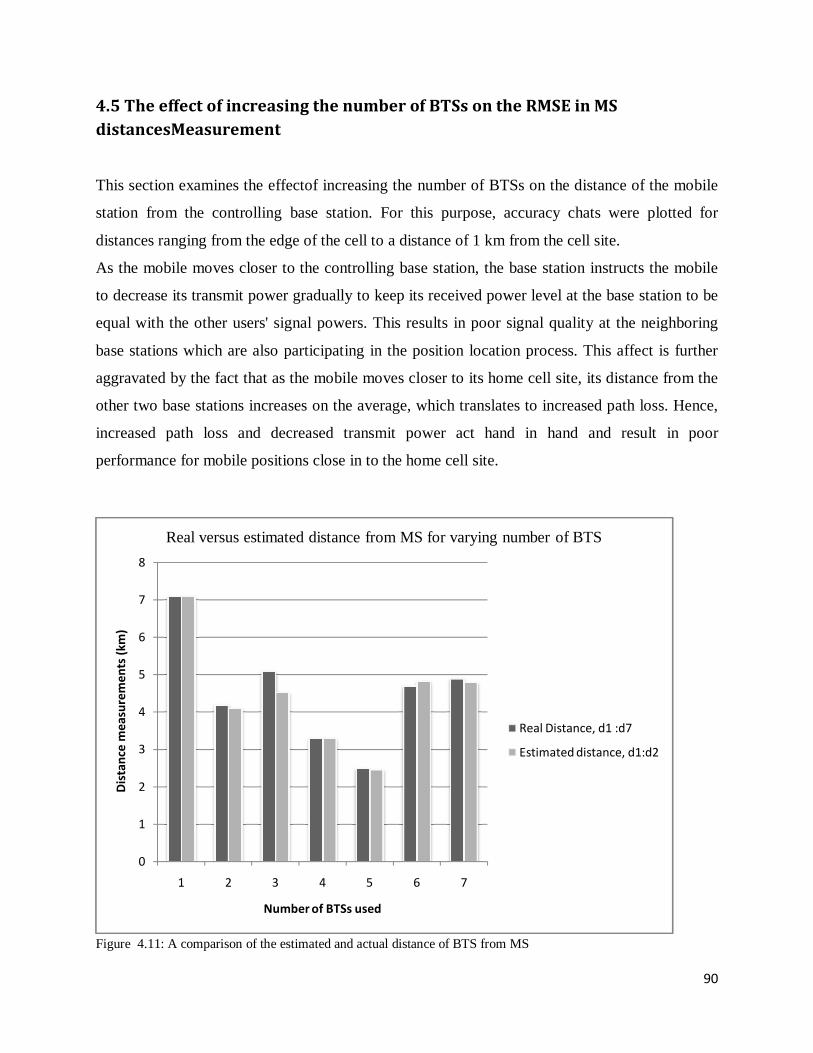
90
4.5 The effect of increasing the number of BTSs on the RMSE in MS distancesMeasurement
This section examines the effectof increasing the number of BTSs on the distance of the mobile
station from the controlling base station. For this purpose, accuracy chats were plotted for
distances ranging from the edge of the cell to a distance of 1 km from the cell site.
As the mobile moves closer to the controlling base station, the base station instructs the mobile
to decrease its transmit power gradually to keep its received power level at the base station to be
equal with the other users' signal powers. This results in poor signal quality at the neighboring
base stations which are also participating in the position location process. This affect is further
aggravated by the fact that as the mobile moves closer to its home cell site, its distance from the
other two base stations increases on the average, which translates to increased path loss. Hence,
increased path loss and decreased transmit power act hand in hand and result in poor
performance for mobile positions close in to the home cell site.
Figure 4.11: A comparison of the estimated and actual distance of BTS from MS
0
1
2
3
4
5
6
7
8
1 2 3 4 5 6 7
Dist
ance
mea
sure
men
ts (k
m)
Number of BTSs used
Real versus estimated distance from MS for varying number of BTS
Real Distance, d1 :d7
Estimated distance, d1:d2
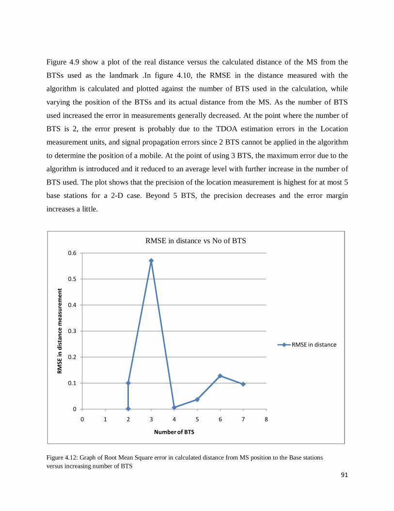
91
Figure 4.9 show a plot of the real distance versus the calculated distance of the MS from the
BTSs used as the landmark .In figure 4.10, the RMSE in the distance measured with the
algorithm is calculated and plotted against the number of BTS used in the calculation, while
varying the position of the BTSs and its actual distance from the MS. As the number of BTS
used increased the error in measurements generally decreased. At the point where the number of
BTS is 2, the error present is probably due to the TDOA estimation errors in the Location
measurement units, and signal propagation errors since 2 BTS cannot be applied in the algorithm
to determine the position of a mobile. At the point of using 3 BTS, the maximum error due to the
algorithm is introduced and it reduced to an average level with further increase in the number of
BTS used. The plot shows that the precision of the location measurement is highest for at most 5
base stations for a 2-D case. Beyond 5 BTS, the precision decreases and the error margin
increases a little.
Figure 4.12: Graph of Root Mean Square error in calculated distance from MS position to the Base stations versus increasing number of BTS
0
0.1
0.2
0.3
0.4
0.5
0.6
0 1 2 3 4 5 6 7 8
RMSE
in d
istan
ce m
easu
rem
ent
Number of BTS
RMSE in distance vs No of BTS
RMSE in distance
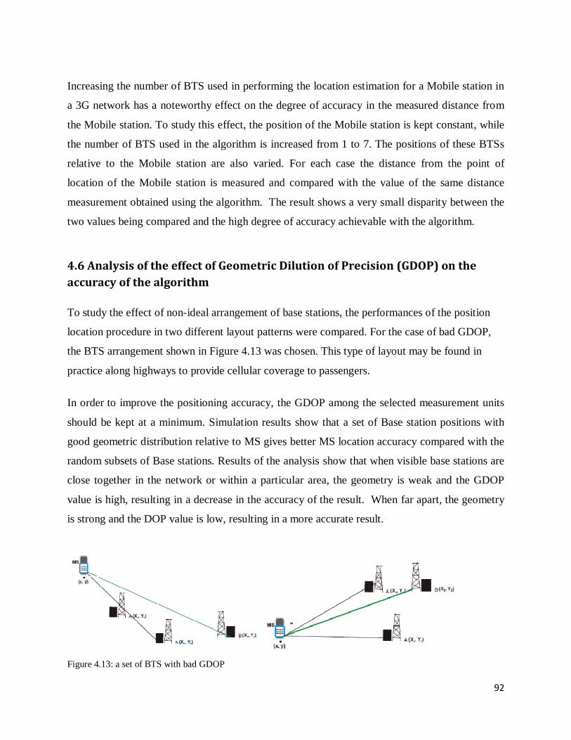
92
Increasing the number of BTS used in performing the location estimation for a Mobile station in
a 3G network has a noteworthy effect on the degree of accuracy in the measured distance from
the Mobile station. To study this effect, the position of the Mobile station is kept constant, while
the number of BTS used in the algorithm is increased from 1 to 7. The positions of these BTSs
relative to the Mobile station are also varied. For each case the distance from the point of
location of the Mobile station is measured and compared with the value of the same distance
measurement obtained using the algorithm. The result shows a very small disparity between the
two values being compared and the high degree of accuracy achievable with the algorithm.
4.6 Analysis of the effect of Geometric Dilution of Precision (GDOP) on the accuracy of the algorithm To study the effect of non-ideal arrangement of base stations, the performances of the position
location procedure in two different layout patterns were compared. For the case of bad GDOP,
the BTS arrangement shown in Figure 4.13 was chosen. This type of layout may be found in
practice along highways to provide cellular coverage to passengers.
In order to improve the positioning accuracy, the GDOP among the selected measurement units
should be kept at a minimum. Simulation results show that a set of Base station positions with
good geometric distribution relative to MS gives better MS location accuracy compared with the
random subsets of Base stations. Results of the analysis show that when visible base stations are
close together in the network or within a particular area, the geometry is weak and the GDOP
value is high, resulting in a decrease in the accuracy of the result. When far apart, the geometry
is strong and the DOP value is low, resulting in a more accurate result.
Figure 4.13: a set of BTS with bad GDOP

93
Figure4.14shows a significant degradation in performance for the case when the threebase
stations lying in a line are used for the TDOA position location. The reason behind this effect is
that in such a case the hyperbolic curves formed by TDOA estimates approacha straight line as
the mobile moves more and more towards positions between any two ofthe base stations.
Therefore, both hyperbolas intersect each other at very small angles.In such a case, even a small
error in TDOA estimation can cause a large position locationerror. Here the distance to three
base stations were measured, and their points were plotted as the intersection of three circles
centered at the Base stations, with the radius calculated as their respective distances to the MS.
The measurement has an error bound as shown in figure 4.14a, and highlighted in figure 4.14b.
The true location of the MS will lie anywhere in the red area. Bad GDOP resulted in the error
bound indicated by the shaded region.
Figure4.14a: Bad GDOP Figure 4.14b: Shaded region could result from bad GDOP
A close cluster or poorly spaced base stations gives poor GDOP value, whereas well distributed
base stations yield good GDOP.
In Figure 4.15, the measurements resulted in two overlapping circles of different centers. If they
overlap at right angles, the greatest extent of the overlap will be much smaller than if they
overlap in near parallel as is the case here.
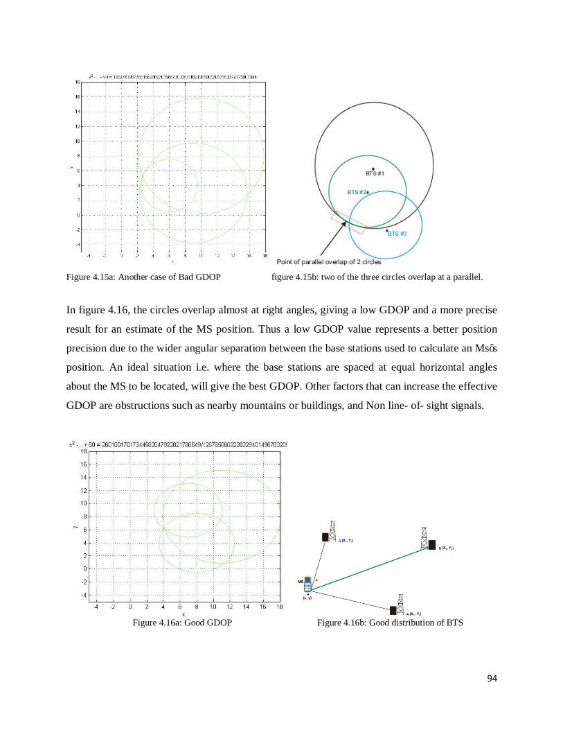
94
Figure 4.15a: Another case of Bad GDOP figure 4.15b: two of the three circles overlap at a parallel.
In figure 4.16, the circles overlap almost at right angles, giving a low GDOP and a more precise
result for an estimate of the MS position. Thus a low GDOP value represents a better position
precision due to the wider angular separation between the base stations used to calculate an Ms’s
position. An ideal situation i.e. where the base stations are spaced at equal horizontal angles
about the MS to be located, will give the best GDOP. Other factors that can increase the effective
GDOP are obstructions such as nearby mountains or buildings, and Non line- of- sight signals.
Figure 4.16a: Good GDOP Figure 4.16b: Good distribution of BTS
95
Excessive measurements increase the computational load and cannot improve the location
accuracy. It could eventually create a problem of redundancy[63].
Mobile location estimation using the proposed algorithm requires a minimum of three base
stations to compute user position. When more number of base stations are in view, best three
base stations i.e. ones with the best GDOP values, are taken in order to reduce redundancy.
In general, the subset with smallest GDOP provides more accurate MS location results. A set of
three or more BSs selected among the visible ones is used to estimate MS location in cellular
communication systems. Those BSs are the ones with the minimum GDOP.
The GDOP can be used as a criterion for selecting a set of base station locations from a large set,
whose measurements produce minimum Position Location estimation error[64].
96
CHAPTER FIVE
CONCLUSION AND RECOMMENDATIONS
Many of the algorithms and methods developed or proposed for locating the position of a user in
a mobile network has been largely unsuccessful to date; having many limitations and shortfalls.
The algorithm presented in this work uses known parameters of the base stations associated with
a mobile user to estimate the position of the unknown user. It avoids the computational
complexities in the use of other algorithms available for the same purpose. A comparison of the
actual and estimated values of the mobile device coordinates showed a very close margin
between the two figures, with an accuracy of over 70% for 90% of the cases tested.
The work done in this research can be extended in many ways. One of the
interestingobservations made in this research was the negative effect of non-ideal base station
arrangement on the Position Location accuracy. It was seen that deviating from the ideal
hexagonal cellular layout increases the effect of errors in TDOA estimation on the overall
position location. The same is the case with the errors in the result of applying the proposed
algorithm.
Since cellular layouts in real situations seldom follow the ideal hexagonal layout, it is logical to
expect that performance in real systems will also degrade as compared to the case withideal
cellular layout. Hence, it would be a useful contribution if practical cellular patternscan be
graded in terms of their GDOP values. In this way, it may be possible to compare different
layout designs from the standpoint of TDOA Position Location and to choose the ones that
arebetter suited for this application. Hence, GDOP measurements may also become a factorfor
choosing cell sites beside the coverage requirements issues.
Another avenue of progress may be to study the application of the algorithm in scenarios where
the mobile station is moving and also different ways of combining informationwhen more than
one position location method is used to locate the mobile unit such as thecombination of AOA
and TDOA methods. It is of importance in such hybrid systems thatthe overall Position Location
estimates should be able to combine the results from both methods in such away that the
inaccuracies in the results from both the methods should not add to each other, thus adversely
97
affecting the overall position location result. The resultant position estimate from the
combinationshould be more accurate than the one obtained from either of the two solutions. Another area of research may be to study the inaccuracies resulting from the totalabsence of a
LOS component in the mobile user's signal. In this study it had been assumed thateven when
there are multiple signal components, there is always a LOS component whichmay, though
sometimes, be weaker than the later arriving components. However, if at least a very weak LOS
component cannot be removed, then the earliest arriving component other than theLOS will be
used to calculate the TDOA values. This would result inerrors in TDOA estimation. The study of
this type of situation is important because therecan be such cases in real environments where
there is no LOS component at all.
Apart from the study of the TDOA method itself, research can also be directed towardssome
related technical issues. There may be some situations when only one base stationis able to
receive the signal from the mobile station under investigation. Such a situation may occur in
rural orsuburban areas where extensive coverage is not needed. One of the solutions proposed
forsuch situations is to use a combination of AOA and TOA methods. A similar technical issue
that can be explored is the effect of additionalposition location data on the data lines between the
base stations and switching center. Ifthe position location process is to be executed only for
emergency calls, then the additional traffic may not be significant. However, if the position
location is performed more often, then theload on the data lines may become significant.
From an application standpoint,it is important to know exactly at which stage of processing
should this procedure beexecuted, and how much additional processing load would it cause for
the switching center.
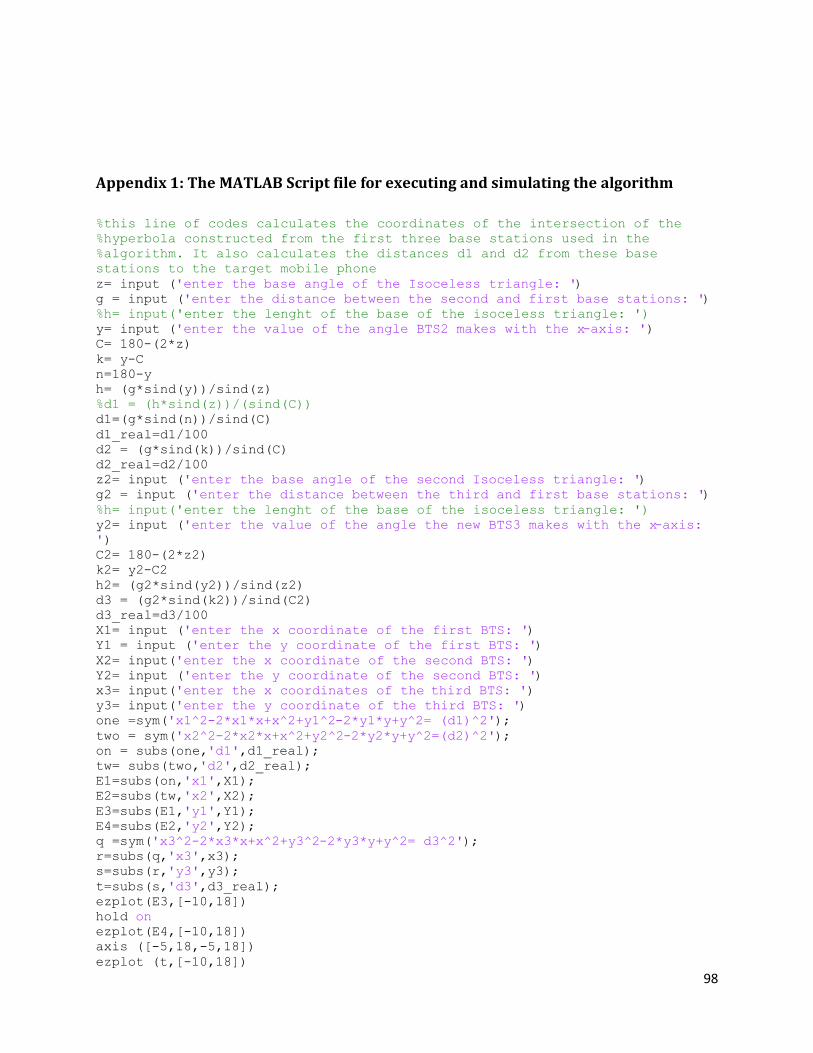
98
Appendix 1: The MATLAB Script file for executing and simulating the algorithm %this line of codes calculates the coordinates of the intersection of the %hyperbola constructed from the first three base stations used in the %algorithm. It also calculates the distances d1 and d2 from these base stations to the target mobile phone z= input ('enter the base angle of the Isoceless triangle: ') g = input ('enter the distance between the second and first base stations: ') %h= input('enter the lenght of the base of the isoceless triangle: ') y= input ('enter the value of the angle BTS2 makes with the x-axis: ') C= 180-(2*z) k= y-C n=180-y h= (g*sind(y))/sind(z) %d1 = (h*sind(z))/(sind(C)) d1=(g*sind(n))/sind(C) d1_real=d1/100 d2 = (g*sind(k))/sind(C) d2_real=d2/100 z2= input ('enter the base angle of the second Isoceless triangle: ') g2 = input ('enter the distance between the third and first base stations: ') %h= input('enter the lenght of the base of the isoceless triangle: ') y2= input ('enter the value of the angle the new BTS3 makes with the x-axis: ') C2= 180-(2*z2) k2= y2-C2 h2= (g2*sind(y2))/sind(z2) d3 = (g2*sind(k2))/sind(C2) d3_real=d3/100 X1= input ('enter the x coordinate of the first BTS: ') Y1 = input ('enter the y coordinate of the first BTS: ') X2= input('enter the x coordinate of the second BTS: ') Y2= input ('enter the y coordinate of the second BTS: ') x3= input('enter the x coordinates of the third BTS: ') y3= input('enter the y coordinate of the third BTS: ') one =sym('x1^2-2*x1*x+x^2+y1^2-2*y1*y+y^2= (d1)^2'); two = sym('x2^2-2*x2*x+x^2+y2^2-2*y2*y+y^2=(d2)^2'); on = subs(one,'d1',d1_real); tw= subs(two,'d2',d2_real); E1=subs(on,'x1',X1); E2=subs(tw,'x2',X2); E3=subs(E1,'y1',Y1); E4=subs(E2,'y2',Y2); q =sym('x3^2-2*x3*x+x^2+y3^2-2*y3*y+y^2= d3^2'); r=subs(q,'x3',x3); s=subs(r,'y3',y3); t=subs(s,'d3',d3_real); ezplot(E3,[-10,18]) hold on ezplot(E4,[-10,18]) axis ([-5,18,-5,18]) ezplot (t,[-10,18])
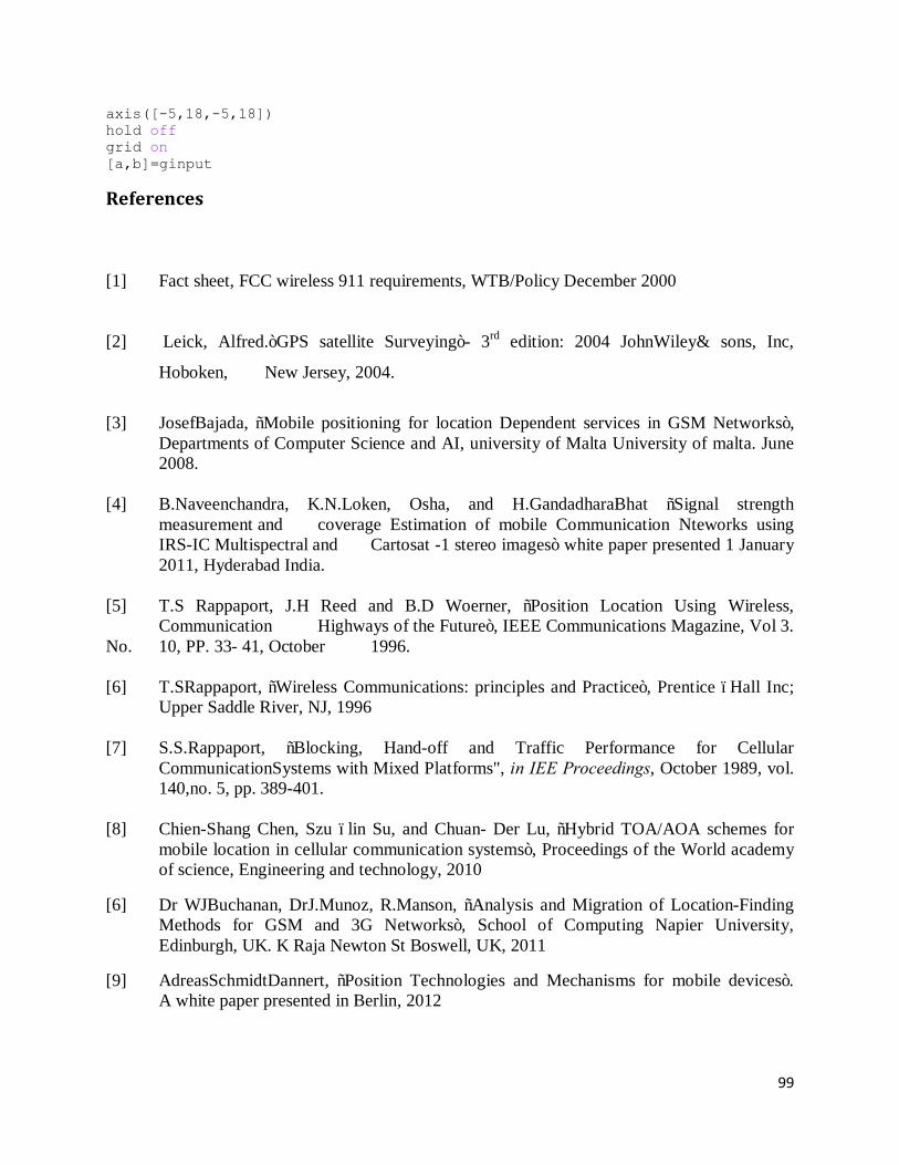
99
axis([-5,18,-5,18]) hold off grid on [a,b]=ginput
References
[1] Fact sheet, FCC wireless 911 requirements, WTB/Policy December 2000
[2] Leick, Alfred.”GPS satellite Surveying”- 3rd edition: 2004 JohnWiley& sons, Inc,
Hoboken, New Jersey, 2004.
[3] JosefBajada, “Mobile positioning for location Dependent services in GSM Networks”,
Departments of Computer Science and AI, university of Malta University of malta. June 2008.
[4] B.Naveenchandra, K.N.Loken, Osha, and H.GandadharaBhat “Signal strength
measurement and coverage Estimation of mobile Communication Nteworks using IRS-IC Multispectral and Cartosat -1 stereo images” white paper presented 1 January 2011, Hyderabad India.
[5] T.S Rappaport, J.H Reed and B.D Woerner, “Position Location Using Wireless, Communication Highways of the Future”, IEEE Communications Magazine, Vol 3. No. 10, PP. 33- 41, October 1996. [6] T.SRappaport, “Wireless Communications: principles and Practice”, Prentice –Hall Inc; Upper Saddle River, NJ, 1996 [7] S.S.Rappaport, “Blocking, Hand-off and Traffic Performance for Cellular CommunicationSystems with Mixed Platforms", in IEE Proceedings, October 1989, vol. 140,no. 5, pp. 389-401. [8] Chien-Shang Chen, Szu –lin Su, and Chuan- Der Lu, “Hybrid TOA/AOA schemes for mobile location in cellular communication systems”, Proceedings of the World academy of science, Engineering and technology, 2010
[6] Dr WJBuchanan, DrJ.Munoz, R.Manson, “Analysis and Migration of Location-Finding Methods for GSM and 3G Networks”, School of Computing Napier University, Edinburgh, UK. K Raja Newton St Boswell, UK, 2011
[9] AdreasSchmidtDannert, “Position Technologies and Mechanisms for mobile devices”. A white paper presented in Berlin, 2012
100
[8] Digital cellular telecommunications system (Phase 2+) (GSM); Universal Mobile Telecommunications System (UMTS);Network architecture(3G TS 23.002 version 3.3.0 Release 1999) European Telecommunications Standards Institute 2000.
[10] Muhammad Farooq et al, “Future Generations of Mobile Communication Networks”, Academy of contemporary research Journal, vol2, issue1, 2013, 24-30)
[11] TarmoAnttalainen, Introduction to Telecommunication Engineering Networks, Artech House publishers, Jan 1, 2003
[12] Transition to 4G, 3GPP Broadband evolution to IMT-Advanced. Release Rysavy Research for 3G Americas, September 2010
[13] Ariel Pashtan, “Wireless terrestrial communications”: cellular telephony, white paper published by Awrae Networks, Inc Buffalo grove, Illinois, USA. 2006 Eolss
[14] AmitKumar, et al, “Evolution of Mobile Wireless Communication Networks:1G to 4G” IJECT Vol. 1, Issue 1, December 2010. I S S N : 2 2 3 0 - 7 1 0 9 (On l i n e )
[15] Ariel Pashtan, “Wireless terrestrial communications: cellular telephony”, a white paper published by Awrae Networks, Inc Buffalo grove, Illinois, USA. 2006 Eolss
[16] TimoHalonen, JavierRomero, and JuanMelero, “GSM, GPRS and EDGE Performance: Evolution towards 3G/UMTS”, Second Edition. John Wiley & Sons Ltd, The Atrium, Southern Gate, Chichester,West Sussex PO19 8SQ, England, 2003
[17] GozalvezSempere, Javier. “An Overview of the GSM System”. Communications Division, Department of Electronic andElectrical Engineering, University of Strathclyde, Glasgow, Scotland. Link: http:www.comms.eee.strath.ac.uk/~gozalvez /gsm/gsm.html.
[18] Heikki Kaaranen et al,“UMTS Networks, architecture, mobility and services”, second edition by JohnWiley and Sons Ltd, 2005
[19] Transition to 4G: 3GPP broadband evolution to IMT-advanced, a white paper published by 3G America, September 2010.
[20] Ariel Pashtan, “Wireless Terrestrial Communications: Cellular Telephony”, an article published by Aware Networks, Inc. Buffalo Grove, Illinois, USA. 2009
[21] Guyton, James. “Wireless Networks in Europe: A Three-Step Evolution”. The Fletcher School of Law & Diplomacy, April 2000.
[22] AmitK.Mogal, “ Wireless Mobile Communication - A Study of 3G Technology”, Department of Computer Science, CMCS College, Nashik-13Int. J. Advanced Networking and ApplicationsVolume: 03 Issue: 05 Pages:01-06 (2012) [23] “2G and 3G mobile communication”, Technical report by iRunway 2013. Accessed at www.i-Runway.com
101
[24] Mathias Erikssson et al, “System Performance with Higher Level Modulation in the GSM/EDGERadio Access Network” Ericsson Radio Systems AB, S-164 80 Stockholm, SwedenEricsson Research, 7001 Development Dr., Research Triangle Park, NC 27709, U.S.A [25] 3GPP group. Universal Mobile Telecommunications System (UMTS); User Equipment (UE) radio transmission and reception (FDD) (3GPP TS 25.101 version 11.3.0 Release 11) ETSI TS 125 101 V11.3.0 (2012- 11). http://www.etsi.org [26] FredericLardinois, “3G, 3.5G, 4G, LTE & WiMAX: Beyond the Marketing Speak”. An article published September 16, 2010 in a series in readwrite sponsored by intel. Address ishttp://readwrite.com/2010/09/16/3g_35g_4g_lte_wimax_ [27] FredericLardinois, “3G, 3.5G, 4G, LTE & WiMAX: Beyond the Marketing Speak”. An article published September 16, 2010 in a series in readwrite sponsored by intel. [28] Ian F. Akyildiz ., DavidM.Gutierrez-Estevez , “The evolution to 4G cellular systems: LTE- Advanced, EliasChavarriaReyes, Physical Communication 3 (2010) 217–244, 2010 Elsevier B.V. journal homepage: www.elsevier.com/locate/phycom [29] “Long-Term Evolution: Simplify the Migration to 4G Networks”, a White Paper by Cisco and its affiliates. 2013 [30] Ishan Shah, NupurMehta, NirjaMehta, RohanShrotriya, “Comparative Study of 4G Technology, Applications and Compatibility in Prevailing Networks”, International Journal of Electronics Communication and Computer Technology (IJECCT) Volume 2 Issue 6 (November 2012) ISSN:2249-7838 IJECCT | www.ijecct.org [31] Sapna Shukla, Varsha Khare, Shubhanshi Garg, Paramanand Sharma, “Comparative Study of 1G, 2G, 3G and 4G”, Journal of Engineering, Computers & Applied Sciences (JEC&AS) ISSN No: 2319‐5606Volume 2, No.4, April 2013. [32] Hellebrandt, M., Mathar, R. and Scheibenbojen, M.; “Estimating position and velocity of mobiles in a cellular Radio Network”, IEEE Transactions on vehicular Technology, Vol. 46, No. 1, Feb. 1997 [33] Munoz, D.; Lara, F.B.; Vargas, C.; Enriquez-Caldera, R.; “Position Location Technique and Applications” 2009, Academic Press ISBN 13:978-0-12 374353-4. [35] Ding Bing Lin; RongTerngJuang; HsinPiaoLin;”Mobile location estimation and tracking for GSM systems” IEEE conferences; Personal. Indoor and mobile Radio Communication. 2004. PIMRC 2004. 15th IEEE International Symposium; Volume: 4; Publication Year: 2004, Page(s): 2835-2839 Vol.4.
102
[36] Massimo Ficco & Stefano Russo; ”A hybrid positioning system for technology Independent location- aware Computing”: softw. Pract. Exper. 2009; 1095-1125. Wiley InterScience.DOI:10.1002/SPE.919. 52 [37] 3GPP TS 25.305 V3.11.0 (2003-12) Technical Specification, 3rd Generation Partnership Project;Technical Specification Group Radio Access Network;Stage 2 functional specification of User Equipment (UE)positioning in UTRAN(Release 1999). [38] F. L. Lewis, “Wireless Sensor Networks”; JohnWiley, New York; ARO Research Grant DAAD 19-02-1-0366; pp: 1-18; year 2004. [39] El-Rabbany, Ahmed. “Introduction to GPS: the Global Positioning System”; 2002. Artech House, INC. ISBN 1-58053-183-1. [40] 3GPP TS 25.305 V3.11.0 (2003-12) Technical Specification, 3rd Generation Partnership Project; Technical Specification Group Radio Access Network; Stage 2 functional specification of User Equipment (UE) positioning in UTRAN (Release 1999) [41] AnthonyClarkson et al;“Hybridized Positioning Algorithms in Location Based Services”. Proceedings of the 1st workshop on positioning, navigation and communication (wpnc’04), Thamesdown Drive, Groundwell,Swindon, Wiltshire, SN25 4XY, UK, 2004 [42] S. Hamani, M. Oussalah, P. Hall;“Combination of GSM and GPS signals for Mobile Positioning and Location Service Using Kalman Filter”, University of Birmingham, Electronics, Electrical and Computer Engineering, Edgbaston, Birmingham B15 2TT. Proceedings of the World Congress on Engineering 2007 Vol II WCE 2007, July 2 - 4, 2007, London, U.K [43] S.Hamani, M.Oussalah, P.;“Hall Position Technologies and Mechanisms for mobile devices”, A white paper presented in 2012 Berlin. [44] A Bahilloet al; “Hybrid RSS-RTT Localization Scheme for Indoor Wireless Networks”, Research Article published inEURASIP Journal on Advances in Signal Processing 2010, Accessed at http://asp.eurasipjournals.com/content/2010/1/126082
[45] Munoz, D.; Lara, F.B.; Vargas, C.; Enriquez-Caldera, R.; “Position Location Technique and Applications” 2009 Academic Press ISBN 13:978-0-12 374353-4. [46] Langley, R.B., “Dilution of Precision, GPS World”, A white paper published in 1999 [47] Proceedings of the 5th WSEAS International Conference on Telecommunications and Informatics, Istanbul, Turkey, May 27-29, 2006 (pp62-69) [48] P.Sravanthi;“Estimation of Mobile Positioning for LBS using GPS-GSM Technology”, International Journal of Advanced Research in Electrical, Electronics and Instrumentation Engineering. Vol. 2, Issue 6, June 2013, ISSN : 2320 – 3765
103
[49] Keeratpal Singh, Mahamod Ismail, Kasmiran Jumari; “A new Technique using Signal Correlation of One Node B to Estimate Mobile Location”, International Journal of Computer Science and Network Security, VOL.8 No.4, Pp 133-139, April 2008
[50] Lubna Farhi; “Dynamic location estimation by kalman filter”, Ubiquitous Computing and Communication Journal Vol. 7, No.5, Pp 1309 -1315,ISSN 1992-8424 [51] MarcoAnisetti et al; ‘”Advanced Localization of Mobile Terminal in Cellular Network”, J. Communications, Network and System Sciences, 2008; 1-103, Published Online February 2008 in SciRes (http://www.SRPublishing.org/journal/ijcns/) [52] Smith J.O, Abel, J.S; “Closed-form least-squares source location estimation from range- difference measurements”, Signal Processing, IEEE Transactions, Vol.52, Issue: 4, Page(s):1121 - 1130, ISSN:1053-587X, 2004
[53] Cheung, K.W et al; “Least squares algorithms for time-of-arrival-based mobile location”, IEEE Transactions,Vol.52, Issue: 4, Pp 1121 - 1130 , ISSN :1053-587X , 2004
[54] M. Abo-Zahhad, Sabah M.Ahmed, M.Mourad;“Hybrid Uplink-Time Difference of Arrival and Assisted-GPS Positioning Technique”,Int. J. Communications, Network and System Sciences, 2012, 5, 303-312
[55] Chien-Shang Chen, Szu –lin Su, and Chuan-Der Lu;“Hybrid TOA/AOA schemes for mobile location in cellular communication systems”, World academy of science, Engineering and technology 2010
[56] Sanem Kabadayi and Ibrahim Tekin;“Software-only TDOA/RTT positioning for 3G WCDMA Wireless network, Wireless Communications and Mobile Computing 2008”; 895–906, Published online 7 August 2007 in Wiley InterScience (www.interscience.wiley.com)
[57] Deng, P., Fan, P.Z.; “An AOA assisted TOA positioning system”, Published in: Communication Technology Proceedings, 2000. WCC - ICCT 2000. International Conference, 2000, Pp 1501 - 1504 vol.2 , 21 Aug 2000-25 Aug 20.00 , Beijing [58] Israel Martin-Escalona and Francisco Barcelo-Arroyo; “A New Time-Based Algorithm for Positioning Mobile Terminals In Wireless Networks”, Research Article published in EURASIP Journal on Advances in Signal Processing, Volume 2008, Article ID 845173, 10 pages, 2007, Spain.
[59] KWCheunget al;“A Constrained Least Squares Approach to Mobile Positioning: Algorithms and Optimality”, EURASIP Journal on Advances in Signal Processing 2006
[60] Adding Location-Based Services to Existing Architectures Building: Feature-Rich Mobile TelephonyApplications Using Dialogic SignalingComponents accessed at http://www.dialogic.com.
104
[61] Liam Smit, Adrie Stander and Jacques Ophoff ; “An Analysis of Base Station Location Accuracy within Mobile-Cellular Networks”, International Journal of Cyber-Security and Digital Forensics (IJCSDF) 1(4): 272-279. The Society of Digital Information and Wireless Communications (SDIWC) 2012 (ISSN: 2305-0012)
[62] 3rd Generation Partnership Project: Technical Specification Group Radio Access Network; Stage 2 functional specification of User Equipment (UE) positioning in UTRAN (Release 1999) [63] V.B.S.Srilatha et al; “Investigation of GDOP for Precise user Position Computation with all Satellites in view and Optimum four Satellite Configurations”, J. Ind. Geophys. Union (July 2009) Vol.13, No.3, pp.139-148 [64] V.B.S.Srilatha, Indira Dutt,et al;“Investigation of GDOP for Precise user Position Computation with all Satellites in view and Optimum four Satellite Configurations”, J. Ind. Geophys. Union (July 2009 ) Vol.13, No.3, pp.139-148
[65] Lassaad Elaabidi, “UMTS, Universal Mobile Telecommunication System”, Cynapsys
Software Engineering, March 2010
[66] System Architecture Evolution (SAE), LTE Resources. Accessed at
http://www.artizanetworks.com/lte_tut_sae_tec.html
[67] Ayad M. H. Khalel, “Position Location Techniques in Wireless Communication Systems”, Electrical Engineering Emphasis on Telecommunications October 2010
[68] L.S Ezema, C.I Ani, G.N Ezeh; “Mobile Location Estimation in GSM?UMTS”, International Journal of Emerging Technology & Research Volume 1, Issue 3, Mar-Apr, 2014 (www.ijetr.org) ISSN (E): 2347-5900 ISSN (P): 2347-6079