ordinal regression models in psychology: a tutorial · inference (liddell & kruschke, 2018)....

https://doi.org/10.1177/2515245918823199

Advances in Methods and Practices in Psychological Science 1 –25© The Author(s) 2019Article reuse guidelines: sagepub.com/journals-permissionsDOI: 10.1177/2515245918823199www.psychologicalscience.org/AMPPS

ASSOCIATION FORPSYCHOLOGICAL SCIENCETutorial

Researchers refer to a variable as an ordinal variable when its categories have a natural order (Stevens, 1946). For example, peoples’ opinions are often probed using items with the following response options: “completely disagree,” “moderately disagree,” “moderately agree,” or “completely agree.” Such ordinal data are ubiquitous in psychology. Although it is widely recognized that ordinal data are not metric, it is commonplace to ana-lyze them with methods that assume metric responses. However, this practice may lead to serious errors in inference (Liddell & Kruschke, 2018). This Tutorial pro-vides a practical and straightforward solution to the perennial issue of analyzing ordinal variables with mod-els that falsely assume the data are metric: flexible and easy-to-use Bayesian ordinal regression models imple-mented in the R statistical computing environment.

What, specifically, is wrong with analyzing ordinal data as if they were metric? This issue was examined in detail by Liddell and Kruschke (2018), whose argu-ments we summarize here. First, analyzing ordinal data with statistical models that assume metric variables, such as t tests and analysis of variance, can lead to low rates of correct detection, distorted effect-size esti-mates, inflated false alarm (Type I error) rates, and even

inversions of differences between groups. There are three main reasons for these problems. First, and most important, the response categories of an ordinal vari-able may not be equidistant—an assumption that is required in statistical models of metric responses; rather, the psychological distance between adjacent response options may not be the same for all such pairs. For example, the difference between “completely dis-agree” and “moderately disagree” may be much smaller in a survey respondent’s mind than the difference between “moderately disagree” and “moderately agree.” Second, the distribution of ordinal responses may be nonnormal, particularly if very low or high values are frequently chosen. Third, variances of the unobserved variables that underlie the observed ordinal variables may differ between groups, conditions, time points, and so forth. Such unequal variances cannot be accounted for—or even detected, in some cases—with the ordinal-as-metric approach.

823199 AMPXXX10.1177/2515245918823199Bürkner, VuorreOrdinal Models in Psychologyresearch-article2019

Corresponding Author:Paul-Christian Bürkner, Department of Psychology, University of Münster, Fliednerstrasse 21, 48149 Münster, Germany E-mail: [email protected]

Ordinal Regression Models in Psychology: A Tutorial

Paul-Christian Bürkner1 and Matti Vuorre2

1Department of Psychology, University of Münster, and 2Department of Psychology, Columbia University

AbstractOrdinal variables, although extremely common in psychology, are almost exclusively analyzed with statistical models that falsely assume them to be metric. This practice can lead to distorted effect-size estimates, inflated error rates, and other problems. We argue for the application of ordinal models that make appropriate assumptions about the variables under study. In this Tutorial, we first explain the three major classes of ordinal models: the cumulative, sequential, and adjacent-category models. We then show how to fit ordinal models in a fully Bayesian framework with the R package brms, using data sets on opinions about stem-cell research and time courses of marriage. The appendices provide detailed mathematical derivations of the models and a discussion of censored ordinal models. Compared with metric models, ordinal models provide better theoretical interpretation and numerical inference from ordinal data, and we recommend their widespread adoption in psychology.

Keywordsordinal models, Likert items, brms, R, open data, open materials

Received 4/4/18; Revision accepted 12/14/18

mailto:[email protected]

https://sagepub.com/journals-permissions

http://crossmark.crossref.org/dialog/?doi=10.1177%2F2515245918823199&domain=pdf&date_stamp=2019-02-25

2 Bürkner, Vuorre

Although these potential pitfalls of applying metric models to ordinal data are widely known, the methods used to deal with them have not been sufficient. For example, one common approach has been to take aver-ages over several Likert items and hope that this aver-aging makes the problems go away. Unfortunately, they do not. Because metric models fail to take into account these issues, and sometimes do not even indicate when there is a problem, we recommend adopting ordinal models instead. In order to determine whether a metric approximation of ordinal data is justified, researchers often have to apply an ordinal model, in which case they can use the results of this ordinal model regardless (Liddell and Kruschke, 2018).

Historically, appropriate methods for analyzing ordi-nal data were limited, although simple analyses, such as comparing two groups, could be performed with nonparametric approaches (Gibbons & Chakraborti, 2011). For more general analyses—regression-like methods, in particular—there were few alternatives to incorrectly treating ordinal data as either metric or nominal. However, using a metric or nominal model with ordinal data leads to over- or underestimating (respectively) the information provided by the data. Fortunately, recent advances in statistics and statistical software have provided many options for appropriate models of ordinal response variables. These methods are often referred to as ordinal regression models. Nev-ertheless, application of these methods remains limited, and the use of less appropriate metric models is wide-spread (Liddell & Kruschke, 2018).

Several reasons may underlie the persistent use of metric models for ordinal data: Researchers might not be aware of more appropriate methods, or they may hesitate to use them because of the perceived complex-ity in applying or interpreting them. Moreover, because closely related (or even the same) ordinal models are referred to with different names in different contexts, it may be difficult for researchers to decide which model is most relevant for their data and theoretical questions. Finally, researchers may also feel compelled to use “standard” analyses because journal editors and reviewers may be skeptical of any “nonstandard” approaches. Therefore, there is need for a review of and practical tutorial on ordinal models to facilitate their use in psychological research. This Tutorial pro-vides such a review and guidance.

The structure of this article is as follows. First, we introduce three common classes of ordinal models. Next, we use two real-world data sets to provide a practical tutorial on fitting ordinal models in the R sta-tistical computing environment (R Core Team, 2017). In the Conclusion, we counter possible objections to using ordinal models and provide practical guidelines

on selecting the appropriate models for different research questions and data sets. In two appendices, we provide detailed mathematical derivations and theo-retical interpretations of the ordinal models and an extension of ordinal models to censored data. We hope that the novel examples, derivations, unifying notation, and software implementation will allow readers to bet-ter address their research questions involving ordinal data.

Classes of Ordinal Models

A large number of parametric ordinal models can be found in the literature. Confusingly, they all have their own names, and their interrelations are often unclear. Fortunately, the vast majority of these models can be categorized within three distinct model classes (Mellenbergh, 1995; Molenaar, 1983; Van Der Ark, 2001): cumulative models, sequential models, and adjacent-category models. We begin by explaining the rationale behind these model classes in sufficient detail to allow researchers to use them and decide which best fits their research question and data. Detailed mathematical deri-vations and discussions are provided in Appendix A.

Cumulative models

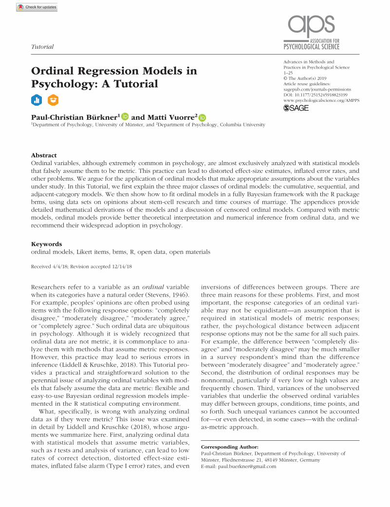
For concreteness, we introduce the class of cumulative models in the context of an example data set of opin-ions about funding stem-cell research. The data set is part of the 2006 U.S. General Social Survey (http://gss .norc.org/) and contains, in addition to opinion ratings, a variable indicating the fundamentalism/liberalism of respondents’ religious beliefs. For our example (taken from Agresti, 2010), we analyze the extent to which religious belief predicts opinions about whether the government should fund stem-cell research, the ordinal dependent variable. The four levels of this Likert item are “definitely not fund” (1), “probably not fund” (2), “probably fund” (3), and “definitely fund” (4).1 This is an ordinal variable because the categories have an ordering, but it is not known what the psychological distance between them is or whether the distances between categories are the same across participants. The assumptions of linear models are violated because the dependent variable cannot be assumed to be con-tinuous or normally distributed. Therefore, we apply an ordinal model to these data, which are summarized in Table 1.

Our cumulative model assumes that the observed ordinal variable Y, the opinion rating, originates from the categorization of a latent (not observable) continu-ous variable Y

∼. In this example, Y

∼ is the latent opinion

about funding stem-cell research. To model this

http://gss.norc.org/

Ordinal Models in Psychology 3

categorization process, the model assumes that there are K thresholds τk, which partition Y into K + 1 observable, ordered categories of Y. In this example, there are four (K + 1 = 4) response categories, and therefore three (K = 3) thresholds. If we assume Y to have a certain distribution (e.g., a normal distribution) with cumulative distribution function F, we can write the probability of Y being equal to category k as

Pr 1( ) ( ) ( ).Y k F Fk k= = τ − τ − (1)

A conceptual illustration of this idea is shown in the top panel of Figure 1. To make this example more concrete, let us suppose we are interested in the prob-ability of k = 2 (“probably not fund”) and have τ −1 1= as well as τ2 1= . Further, we assume Y to be normally distributed with a standard deviation fixed to 1, and we call the corresponding cumulative normal distribution function Φ (see Fig. A1 in Appendix A for a graph comparing this function with other common functions). Then, we compute

Pr 2 1 1

84 16 682 1( ) ( ) ( ) ( ) ( )

. . . .

Y = = == =Φ Φ Φ Φτ − τ − −

− (2)

However, Equation 2 does not yet describe a regres-sion model, because there are no predictor variables. We therefore formulate a linear regression for Y with predictor term η = b1x1 + b2x2 + . . ., so that Y = η ε+ , where ε describes the error term of the regression. Consequently, Y is split into two parts. The first one (η) represents variation in Y that can be explained by the predictors, and the second one (ε) represents varia-tion that remains unexplained. Note that there is no intercept in the predictor term, because the thresholds τk replace the model’s intercept, as the thresholds and intercept are not identified at the same time. Thus, we model the probabilities of Y being equal to category k given the linear predictor η:

Pr 1( | ) ( ) ( ).Y k F Fk k= =η τ − η − τ − η− (3)

We provide a more detailed description and derivation of the general cumulative model in Appendix A.

The categorization interpretation is natural for many Likert-item data sets, in which ordered verbal (or numerical) labels are used to obtain discrete responses about a possibly continuous psychological variable. Given the widespread use of Likert items in psychology, cumulative models are possibly the most important class of ordinal models for psychological research. It is reasonable to assume that the stem-cell opinion ratings result from categorization of a latent continuous variable—the individual’s opinion about stem-cell research. Therefore, a cumulative model is theoretically motivated and justified for the data in this example.

We wish to predict funding opinion Y from religious belief, which has categories “moderate,” “liberal,” and “fundamentalist.” In the regression model, we use dummy coding with “moderate” as the reference cate-gory. Thus, we have two numerical predictor variables, x1 and x2, and the corresponding regression coeffi-cients, b1 and b2, have the following interpretation: b1 is the contrast between moderate and liberal religious belief, and b2 is the contrast between moderate and fundamentalist religious belief. The regression model of individuals’ latent opinions about stem-cell research is thus

Y b x b xk .= + = + +η ε ε1 1 2 2 (4)

We assume the latent variable Y (or, equivalently, the error term ε) to be normally distributed2 with a standard deviation fixed to 1. As before, we call the corresponding cumulative normal distribution function Φ. Then, the probability for each response category k can be computed as follows:

Pr 1 1 2 2 1 1 1 2 2( ) ( ( )) ( ( )).Y k b x b x b x b xk k= = +Φ Φτ − + − τ −− (5)

The parameters to be estimated are the three thresh-olds, τ1 to τ3 , as well as the two regression coefficients, b1 and b2. In the next main section, we show how to fit this model in the R programming environment.

Sequential models

We introduce the class of sequential models in the context of a real-life data set concerning marriage dura-tion. The data are from the 2013–2015 U.S. National

Table 1. Frequencies of Opinion Ratings in the Stem-Cell Data Set

Opinion ratinga

Religious belief 1 2 3 4

Fundamentalist 40 54 119 55Moderate 25 41 135 71Liberal 23 31 113 122

aParticipants were asked whether the government should fund stem-cell research, and the response options were as follows: 1 = “definitely not fund”; 2 = “probably not fund; 3 = “probably fund”; 4 = “definitely fund.”

4 Bürkner, Vuorre

Survey of Family Growth (NSFG; Centers for Disease Control and Prevention, n.d.), in which data about fam-ily life were gathered for more than 10,000 individuals. We focus on a sample of 1,597 women who had been married at least once in their life at the time of the survey. Inspired by Teachman (2011), who used the NSFG 1995 data, we are interested in predicting the duration, in years, of first marriage. For now, we con-sider only divorced couples in order to illustrate the main ideas of a sequential model. If we included non-divorced women in the data, their data would be called censored because the event (divorce) was not observed. Although sequential models can be used to model cen-sored data, we defer this additional complexity to Appendix B. The first 10 rows of the data are shown in Table 2.

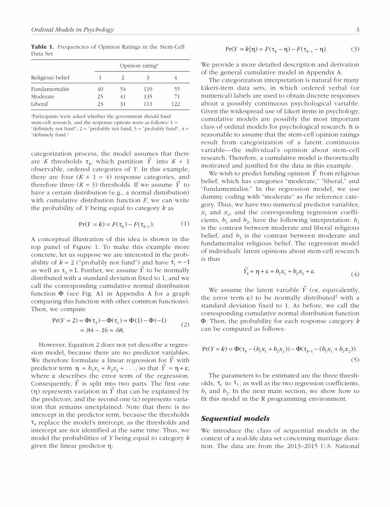
For many ordinal variables, the assumption of a single underlying continuous variable, as in cumulative models, may not be appropriate. If the response can be understood as being the result of a sequential pro-cess, such that a higher response category is possible only after all lower categories are achieved, the sequen-tial model proposed by Tutz (1990) is usually appropri-ate. For example, a couple can divorce in the 7th year only if they have not already divorced in their first 6 years of marriage: Duration of marriage in years—the ordinal dependent variable Y in the current example—can be thought of as resulting from a sequential process.

Sequential models assume that for every category k—year of marriage in our example—there is a latent continuous variable Yk that determines the transition

Y = 1 Y = 2 Y = 3 Y = 4

Y = 1 Y > 1 Y = 2 Y > 2 Y = 3 Y > 3

Y = 1 Y = 2 Y = 2 Y = 3 Y = 3 Y = 4

τ 1 τ 2 τ 3

τ 1 τ 2 τ 3

τ 1 τ 2 τ 3

Y1~

Y2~

Y3~

Y1~

Y2~

Y3~

Y~

Cumulative Model

Sequential Model

Adjacent-Category Model

Fig. 1. Illustration of the assumptions of the classes of ordinal models: cumulative models, sequential models, and adjacent-category models. Each type of model divides the latent continuous variable, Y , into bins according to thresholds τ. The area under the curve in each bin represents the prob-ability of the corresponding event (observed ordinal response Y) given the set of possible events for the latent variable. (See the main text and Appendix A for more detailed descriptions of these three model classes.)


between the kth and the k + 1th category. In the mar-riage example, Yk represents all the factors contributing to the probability of a couple’s marriage continuing beyond a given year k. Informally, we could call Yk “marriage quality” in this example. The categories are separated by thresholds τk—perhaps thought of as the combination of all factors working against the marriage continuing beyond year k. If Yk is greater than the thresh-old τk, the sequential process—in this case, marriage—continues; otherwise, it stops at category k. The general concept underlying the class of sequential models is illustrated in the middle panel of Figure 1.

Because the thresholds τk refer to different latent variables, they do not need to be ordered. That is, τk+1 may be either greater than or less than τk. Much as we did in the derivation of our cumulative model, we need to assume a certain distribution for Yk (e.g., a normal distribution) with cumulative distribution function F. Let us suppose we want to model the probability of divorce in the 3rd year. This means that divorce did not happen in the 1st year ( Y1 > τ1), did not happen in the 2nd year ( Y2 > τ2), but did happen in the 3rd year ( Y3 ≤ τ3). We can write this as follows:

Pr( 3) Pr Pr Pr

1 Pr 1 Pr

1 2 3

1

Y Y Y Y

Y

= = > > ≤

= ≤

( ) ( ) ( )

( ( ))(

1 2 3

1

τ τ τ

− τ − (( )) ( ). Y Y2 3≤ ≤τ τ2 3Pr (6)

If we further assume Y1, Y2, and Y3 to be standard normally distributed and set, just for illustration purposes, the threshold values as τ1 = 0, τ2 = –1, and τ3 = 1, we can explicitly compute the probability of divorce in the 3rd year:

Pr( 3) 1 1

1 1 1 1 351 2 3Y = =

= =

( ( ))( ( )) ( )

( ( ))( ( )) ( ) . .

− τ − τ τ

− − −

Φ Φ Φ

Φ Φ Φ0 (7)

To make this sequential model an actual regression model, we set up a linear regression for each latent variable via Yk k= η + ε , which includes a category-specific error term (i.e., εk). By default, all Yk share the same linear predictor η, such that the effect of any potential predictor is constant across k (e.g., age at marriage is related to Yk identically for years k = 3 and k = 9.) This implies the following probability for cate-gory k:

Pr |( ) ( ) ( ( )).Y k F Fkj

k

j= = − − −=

−

∏η τ η τ η1

1

1 (8)

In words, the probability that Y falls in category k is equal to the probability that it did not fall in one of the former categories 1 to k – 1, multiplied by the probabil-ity that the sequential process stopped at k rather than continuing beyond it. In the current example, we use the survey respondents’ age at marriage and whether the couple was already living together before marriage as predictors of marriage duration. We can think of the years of marriage as a sequential process: Each year, the marriage may continue or end by divorce, but the latter can happen only if it did not happen before. The number of years of marriage until divorce is our response variable Y, whereas age at marriage and whether the couple was already living together before marriage are our predictor variables, which we denote as x1 and x2, respectively. As the latter predictor is cat-egorical, for our analysis it is dummy coded as 1 if the couple was already living together and as 0 otherwise.

Table 2. First 10 Rows of the Marriage Data From the 2013–2015 U.S. National Survey of Family Growth (Centers for Disease Control and Prevention, n.d.)

Couple (coded as ID)

Couple lived together before

marriage? (coded as together)

Woman’s age at marriage (coded as age)

Duration of marriage (coded as years)

Divorced at time of survey

(coded as divorced)

1 Yes 19 9 True2 Yes 22 9 False3 Yes 20 5 False4 Yes 22 2 False5 Yes 25 6 False6 Yes 30 1 False7 Yes 32 9 False8 No 24 14 True9 No 37 1 True10 Yes 18 13 True

Note: In the main analysis, only data of divorced women were used.

6 Bürkner, Vuorre

This implies the following linear regression for the latent variables Yk:

Y b x b xk k .= + +1 1 2 2 ε (9)

We assume an extreme-value distribution for Yk (F = EV), because it is the most common choice in

discrete time-to-event, or survival, models. This func-tion is graphically compared with other alternatives in Figure A1 in Appendix A. Together, these assumptions imply that the probability of a marriage ending in the kth year can be computed as follows:

Pr( ) ( ( ))

( ( ( ))).

Y k EV b x b x

EV b x b x

k

j

k

j

= = − +

− − +=

−

∏

τ

τ

1 1 2 2

1

1

1 1 2 21 (10)

For the current data set, the longest marriage ended in divorce after 27 years, so we have 26 thresholds (τ1 to τ26) to estimate in addition to the two regression coefficients, b1 and b2. In the next main section, we show how to fit this model in the R programming environment.

Adjacent-category models

Adjacent-category models are widely used in item response theory and are applied in many large-scale assessment studies, such as the Program for Interna-tional Student Assessment (PISA; OECD, 2017). They are somewhat different from cumulative and sequential models because it is difficult to think of a natural pro-cess leading to them. Therefore, an adjacent-category model can be chosen for its mathematical convenience rather than any quality of interpretation. Consequently, we do not present a practical example specifically dedi-cated to this approach, but we illustrate its use when we fit ordinal models to the stem-cell data set. Adjacent-category models predict the decision between two adja-cent categories k and k + 1 using latent variables Yk, with thresholds τk and cumulative distribution function F. If Yk < τk, we choose category k; otherwise, we choose category k + 1. The decision process assumed by adjacent-category models is illustrated in the bottom panel of Figure 1. We can formally write this as follows:

Pr 1Y k Y k k F k= ∈ +{ }( ) =| , ( ).τ (11)

This is superficially similar to the form of sequential models, but with an important distinction. Sequential models model the decision between Y = k and Y > k, whereas adjacent-category models model the decision between Y = k and Y = k + 1. Suppose that the latent variable Y2 is standard normally distributed (with dis-tribution function Φ) and τ2 = 1. In this case, the

probability of choosing Y = 2 (“probably not fund”) over Y = 3 (“probably fund”) in the stem-cell example would be written as follows in an adjacent-category model:

| , ( ) ( ) . .Pr 2 2 3 1 842Y Y= ∈{ }( ) = = =Φ Φτ (12)

Including the linear predictor η in this model leads to the following general equation:

Pr 1Y k Y k k F k= ∈ +{ }( ) =| , , ( ).η τ − η (13)

The (unconditional) probability of the response Y being equal to category k given η (i.e., Pr(Y = k|η)) is com-puted with a quite extensive formula, shown in Appen-dix A.

Generalizations of ordinal models

We have introduced the three most important classes of ordinal models and refer readers to Appendix A for more details on each of them. Box 1 provides an over-view of these three model classes and how to apply them with the software package described in the next main section. However, before discussing how to fit ordinal models in R, we briefly consider generalizations of these model classes to handle category-specific effects and unequal variances.

Category-specific effects. In all of the ordinal models we have described thus far, all predictors are by default assumed to have the same effect on all response catego-ries, which may not always be an appropriate assump-tion. It is often possible that a predictor has different effects on different response categories of Y. For exam-ple, religious belief may have little relation to whether people choose “definitely not fund” over “probably not fund” in rating their opinion about funding stem-cell research, but may strongly predict whether they choose “probably fund” over “definitely fund.” In such a case, one can model the predictor as having category-specific effects by estimating not one but K coefficients for it. Doing so is unproblematic in sequential and adjacent-category models, but may lead to negative probabilities, and thus problems in model fitting, in cumulative models (see Appendix A).

Unequal variances. Especially in the context of cumulative models, the response function F is usually assumed to be a standard normal distribution, that is, to have a variance ν of 1 for reasons of model identification. Freely varying ν is not possible in ordinal models if all the thresholds τ are allowed to vary as well. However, it is possible for ν to vary as a function of group, condition, time, or any other predictor variable (i.e., for Y to have


Consider an observed ordinal response variable Y and a predictor X. The three model classes can be summarized as follows:

1. Cumulative model

• Y originates from categorization of a latent variable Y .• Basic code for implementing a cumulative model: brm(Y X, family = cumulative(), ...),• Example: Using gender to predict responses to a 5-point Likert item

2. Sequential model

• Y is the result of a sequential process.• Basic code for implementing a sequential model: brm(Y

X, family = sratio(), ...)

• Example: Using age to predict the number of cars people have bought

3. Adjacent-category model

• Y is modeled as the decision between two adjacent categories of Y .• Basic code for implementing an adjacent-category model: brm(Y X, family = acat(), ...),• Example: Predicting the number of correctly solved subitems in a complex math task


1. Category-specific effects can be modeled with sequential and adjacent-category models.

• Basic code for modeling category-specific effects: brm(Y cs(X), family = acat()/sratio(), ...)• Example: Using gender to predict responses to Likert items when gender is expected to affect responses high on the

rating scale differently than responses low on the rating scale

2. Unequal variances can be modeled with all three classes of ordinal models.

• Basic code for modeling unequal variances: brm(bf(Y X, disc X), ...)

• Example: Using gender to predict responses to Likert items when the variances of the latent variables differ between genders

Note: ... indicates additional arguments to brm(), such as specifying a data set.

Box 1. Overview of the Three Classes of Ordinal Models and How to Apply Them With brms Syntax

unequal variances across groups, conditions, etc.) pro-vided that the baseline variance is fixed to some value. Ignoring the possibility of unequal variances can lead to problems such as inflated error rates and distorted effect sizes (Liddell & Kruschke, 2018). Fortunately, unequal variances are easily incorporated into the ordinal models, as we show later.

Disclosures

The complete R code for this Tutorial and the example data used here are available at the Open Science Frame-work (https://osf.io/cu8jv/).

Fitting Ordinal Models in R

Although a number of software packages in the R sta-tistical programming environment (R Core Team, 2017) allow modeling ordinal responses, here we use the brms (Bayesian regression models using ‘Stan’) package (Bürkner, 2017, 2018; Carpenter et al., 2017), for two main reasons. First, it can estimate all three ordinal model classes we have introduced in combination with multilevel structures, category-specific effects (though not in the case of cumulative models), unequal vari-ances, and more. Second, brms estimates models in a Bayesian framework, which provides considerably

more information about the models and their param-eters than the frequentist approach (Gelman et al., 2013; McElreath, 2016), allows a more natural quanti-fication of uncertainty (Kruschke, 2014), and makes it possible to estimate models when traditional methods based on maximum likelihood fail (Eager & Roy, 2017). A brief description of the basic concepts of Bayesian statistics is provided in Box 2 (see also Kruschke & Liddell, 2018a, 2018b). We provide brief notes on imple-menting ordinal models using other software packages in our concluding section.

In this section, we assume that readers know how to load data sets into R and execute other basic com-mands. Readers unfamiliar with R may consult free online R tutorials.3 To follow the examples in this sec-tion, users first need to install the brms R package. Packages should be installed only once, and therefore the following code snippet, which installs brms, should be run only once:

install.packages("brms")

In order to have the brms functions available in the current R session, users must load the package at the beginning of every session:

library(brms)

https://osf.io/cu8jv/

8 Bürkner, Vuorre

Bayesian statistics focuses on the posterior distribution p(θ|Y), where θ are the model parameters (unknown quantities) and Y are the data (known quantities) to condition on. The posterior distribution is generally computed as

p Yp Y p

p Y( | )

( | ) ( )

( ).θ

θ θ=

In this equation, p(Y|θ) is the likelihood, p(θ) is the prior distribution, and p(Y) is the marginal likelihood. The likelihood p(Y|θ) is the distribution of the data given the parameters and thus relates the data to the parameters. The prior distribution p(θ) describes the uncertainty in the parameters before the data have been seen. It thus allows explicit incorporation of prior knowledge into the model. The marginal likelihood p(Y) serves as a normalizing constant so that the posterior is an actual probability distribution. Except in the context of specific methods (i.e., Bayes factors), p(Y) is rarely of direct interest.

In classical frequentist statistics, parameter estimates are obtained by finding those parameter values that maximize the likelihood. In contrast, Bayesian statistics estimate the full (joint) posterior distribution of the parameters. Estimating the full posterior distribution not only is fully consistent with probability theory, but also is much more informative than estimating a single point (with an approximate measure of uncertainty commonly known as standard error).

Obtaining the posterior distribution analytically is rarely possible, and thus Bayesian statistics relies on Markov-Chain Monte Carlo methods to obtain samples (i.e., random values) from the posterior distribution. Such sampling algorithms are computationally very intensive, and thus fitting models using Bayesian statistics is usually much slower than fitting models using frequentist statistics. However, the advantages of Bayesian statistics—such as greater modeling flexibility, inclusion of prior distributions, and more informative results—are often worth the increased computational cost.

Box 2. Basics of Bayesian Statistics

Next, we discuss analyses of two real-world data sets (from different areas of psychology) in which the main dependent variable is an ordinal variable. We remind readers that ordinal data are not limited to the types of variables discussed here, but can be found in a wide variety of research areas, as noted by Stevens (1946): “As a matter of fact, most of the scales used widely and effectively by psychologists are ordinal scales” (p. 679).

Opinions about funding stem-cell research

First, we analyze the stem-cell data set introduced ear-lier (see Table 1). We wish to predict the respondents’ opinions about funding stem-cell research (coded as rating) from the degree of fundamentalism of their religious beliefs (coded as belief). This model can easily be fitted by including three arguments in the brm() function, as follows:

fit_sc1 <- brm(

formula = rating ~ 1 + belief,

data = stemcell,

family = cumulative("probit")

)

The three arguments inside brm() are formula, data, and family, respectively. First, and perhaps most important, the formula argument identifies

which variable (or variables) is the dependent variable, and which variable (or variables) is the predictor vari-able. The model’s formula is specified with standard R modeling syntax, in which dependent variables are written on the left-hand side of ~ and predictors are written on the right-hand side; predictors are separated by + unless an interaction between predictors is desired, in which case they are separated by inserting *, rather than +. The 1 on the right-hand side of ~ means that an intercept (i.e., the threshold in an ordinal model) should be included. Although it is included automati-cally, we added this notation here for clarity. Note also that arguments do not have to be named because R functions allow the arguments to be specified in order; if arguments are not named, they will be applied in the expected order.

In addition, this function includes data and family arguments. The former takes a data frame from the cur-rent R environment. The latter defines the distribution of the response variable, that is, the specific ordinal model to be used and the transformation to be applied to the predictor term—which is nothing other than the distribution function F in ordinal models. We have speci-fied cumulative(“probit”) in order to apply a cumulative model assuming the latent variable (or, equivalently, the error term ε) to be normally distributed. If we had omitted probit from the specification of the family, the default logistic distribution would have been assumed instead (see Appendix A for a visualization).

The model (which we have saved into the fit_sc1 variable) is readily summarized via


summary(fit_sc1)

## Family: cumulative

## Links: mu = probit; disc = identity

## Formula: rating ~ 1 + belief

## Data: stemcell (Number of observations: 829)

## Samples: 4 chains, each with iter = 2000; warmup = 1000; thin = 1;

## total post-warmup samples = 4000

##

## Population-Level Effects:

## Estimate Est.Error l-95% CI u-95% CI Eff.Sample Rhat

## Intercept[1] -1.25 0.08 -1.42 -1.10 2681 1.00

## Intercept[2] -0.64 0.07 -0.78 -0.50 3629 1.00

## Intercept[3] 0.57 0.07 0.43 0.71 3461 1.00

## belieffundamentalist -0.24 0.09 -0.43 -0.06 3420 1.00

## beliefliberal 0.31 0.09 0.13 0.50 3381 1.00

##

## Samples were drawn using sampling(NUTS). For each parameter, Eff.Sample

## is a crude measure of effective sample size, and Rhat is the potential

## scale reduction factor on split chains (at convergence, Rhat = 1).

For consistency with other model classes that brms supports, thresholds in ordinal models are called “inter-cepts” although, from a theoretical perspective, they are not quite the same. In addition to the regression coefficients (which are displayed under the heading Population-Level Effects), this display includes information about the model (first three rows), the data, and the Bayesian estimation algorithm (Samples row; for additional information about this algorithm, see, e.g., Betancourt, 2017; Bürkner, 2017; van Ravenzwaaij, Cassey, & Brown, 2018).

Of most importance for present purposes are the regression coefficients. The Estimate column pro-vides the posterior means of the parameters, and the Est.Error column shows the parameters’ posterior standard deviations. These quantities are analogous, but not identical, to frequentist point estimates and standard errors, respectively. The l-95% CI and u-95% CI columns provide the lower and upper bounds of the 95% credible intervals, or CIs, which are Bayesian confidence intervals (the numbers refer to the 2.5th and 97.5th percentiles of the posterior

distributions). Although credible intervals can be numerically similar to their frequentist counterparts, confidence intervals, they actually lend themselves to an intuitive probabilistic interpretation, unlike confi-dence intervals, which are often mistakenly so inter-preted (Hoekstra, Morey, Rouder, & Wagenmakers, 2014; Morey, Hoekstra, Rouder, Lee, & Wagenmakers, 2016). To get different credible intervals, one can use the prob argument (e.g., summary(fit_sc1, prob = .99) will yield 99% CIs).

The two additional columns, named Eff.Sample (effective sample size) and Rhat, indicate whether the model-fitting algorithm converged to the underlying values and are briefly explained in the last three rows of the output. In short, Rhat should not be larger than 1.1, and Eff.Sample should be as large as possible. For most applications, an effective sample size greater than 1,000 is sufficient for stable estimates. Because these quantities are not the focus of this Tutorial—and convergence is not a problem for any of the models considered here—we refer readers to Bürkner (2017) for more details.

10 Bürkner, Vuorre

The first three rows of the output under Population-Level Effects describe the three thresholds of the cumulative model as applied to the stem-cell opinion data. Recall that when the cumulative distribution func-tion F is Φ (standard normal distribution), Y is a stan-dard normal variable. Consequently, the thresholds indicate where the continuous latent variable Y is par-titioned to produce the observed responses Y, in stan-dard-deviation units. Therefore, applying Φ to each threshold leads to the cumulative probability of responses below that threshold if all predictor variables were zero. Although it is important to be able to interpret the thresholds, they are rarely of central focus in modeling (much as ordinary regression intercepts are rarely of central focus). Instead, we are most interested in the regression coefficients b1 and b2, to which we turn next.

Because religious belief was coded as a factor in R with “moderate” as the reference category, the coefficients belieffundamentalist and beliefliberal indicate the extent to which people with fundamentalist and liberal religious beliefs differed from those with moderate beliefs on the latent scale of opinion regard-ing funding stem-cell research. The point estimate of beliefliberal indicates that on the latent opinion scale, people with liberal beliefs held opinions that were 0.31 SD more positive toward funding stem-cell research compared with the opinions of moderates. The 95% CI of this parameter is between 0.13 and 0.50, and so does not include zero. We can therefore conclude with at least 95% probability that people with liberal religious beliefs held more positive opinions regarding the funding of stem-cell research than did people with moderate religious beliefs.

People with fundamentalist religious beliefs, on the other hand, had more negative opinions regarding funding stem-cell research than did people with moder-ate religious beliefs. On the latent opinion scale, fun-damentalists’ opinions about funding stem-cell research were 0.24 SD more negative than the opinions of peo-ple with moderate religious beliefs. This parameter is between −0.43 and −0.06 with 95% probability.

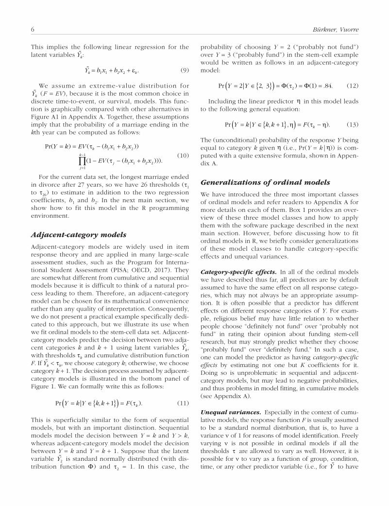
The results can also be summarized visually by plot-ting the estimated relationship between religious belief and response to the opinion question. Figure 2 displays the estimated probabilities of the four response catego-ries for the three religious-belief groups. It is quite clear from the figure that fundamentalists were less likely to respond “definitely fund” (4) than were either of the other two groups. Similarly, they were more likely to respond “definitely not fund” (1) and “probably not fund” (2) than the other two groups were. The code to produce this figure is as follows:

marginal_effects( fit_sc1, "belief", categorical = TRUE)

Category-specific effects. Thus far, we assumed that the effect of religious belief was equal across the opinion rating categories. That is, there was only one predictor term for the effect of fundamentalist and liberal beliefs on funding opinion. However, this assumption may not be appropriate, and beliefs may affect opinions differ-ently depending on the rating category. For example, it is possible that individuals with liberal beliefs are more likely to respond with the highest rating than are

.1

.2

.3

.4

.5

Moderate Fundamentalist LiberalBelief

Probability

Rating

1234

Fig. 2. Marginal effects of religious belief on opinion about funding stem-cell research, from model fit_sc1 (data from the 2006 U.S. General Social Survey, http://gss.norc.org/). The posterior mean estimate of the probability of responses in each opinion rating category is shown for each of the three groups (moderate, fundamentalist, and liberal). Error bars indicate 95% credible intervals.

http://gss.norc.org/


individuals with moderate beliefs, but that the two groups do not otherwise differ in their opinion ratings. When the effects of predictors can vary in this manner across cate-gories, the resulting model is said to have category-specific effects.

Next, we consider whether religious belief has cat-egory-specific effects in this data set. In other words, does its relationship to funding opinion vary across response categories? Fitting category-specific effects in cumulative models is problematic because of the pos-sibility of negative probabilities (see Appendix A) and consequently is not allowed in brms. Therefore, we use an adjacent-category model instead. To specify an adjacent-category model, we use family = acat() instead of family = cumulative() as an argument to the brm() function. Then, to model religious belief with possible category-specific effects, we wrap this variable in cs() in the model’s formula:

fit_sc2 <- brm(

formula = rating ~ 1 + cs(belief),

data = stemcell,

family = acat("probit")

)

As indicated in Table 3, liberals preferred “definitely fund” (4) over “probably fund” (3) much more than moderates did, b = 0.45 (95% CI = [0.21, 0.68]). At the

same time, there was little difference between liberals and moderates for the other response categories. In contrast, fundamentalists preferred lower response cat-egories than moderates across the rating scale, but the differences were quite small and uncertain—as indi-cated by the rather wide 95% CIs, which also overlap zero.

It can be more difficult to interpret the sizes of coef-ficients from an adjacent-category model, compared with coefficients from a cumulative model. Thus, we recommend plotting an adjacent-category model’s pre-dicted values (e.g., via marginal_effects(fit_sc2)), so that the magnitudes of the effects can be better understood. With the stem-cell data, the resulting figure looks very similar to Figure 2, and thus we do not show it here.

Unequal variances. As we noted earlier, it is usually assumed that the variance of the latent variable is the same throughout the model. Within the framework of ordinal models in brms, we can relax this assumption.4 For the stem-cell data, this implies asking whether the variances of funding opinions differ across categories of religious belief.

Conceptually, unequal variances are incorporated in the model by specifying an additional regression for-mula for the variance component of the latent variable Y . In brms, the parameter related to latent variances

is called disc (short for “discrimination”), following

Table 3. Summary of the Regression Coefficients for the Category-Specific Adjacent-Category Model Fitted to the Stem-Cell Data Set

Predictor Estimate95% credible

interval

First threshold (coded as Intercept[1]) –0.32 [–0.62, 0.01]Second threshold (coded as Intercept[2]) –0.73 [–0.94, –0.52]Third threshold (coded as Intercept[3]) 0.40 [0.22, 0.58]Fundamentalists’ vs. moderates’ preference for “2” over “1”

(coded as belieffundamentalist[1])–0.13 [–0.53, 0.28]

Fundamentalists’ vs. moderates’ preference for “3” over “2” (coded as belieffundamentalist[2])

–0.24 [–0.54, 0.04]

Fundamentalists’ vs. moderates’ preference for “4” over “3” (coded as belieffundamentalist[3])

–0.08 [–0.33, 0.19]

Liberals’ vs. moderates’ preference for “2” over “1” (coded as beliefliberal[1])

–0.12 [–0.57, 0.34]


0.06 [–0.25, 0.36]


0.45 [0.21, 0.68]

Note: Participants were asked whether the government should fund stem-cell research, and the response options were as follows: 1 = “definitely not fund”; 2 = “probably not fund”; 3 = “probably fund”; 4 = “definitely fund.” The reference category for liberals and fundamentalists was moderates.

12 Bürkner, Vuorre

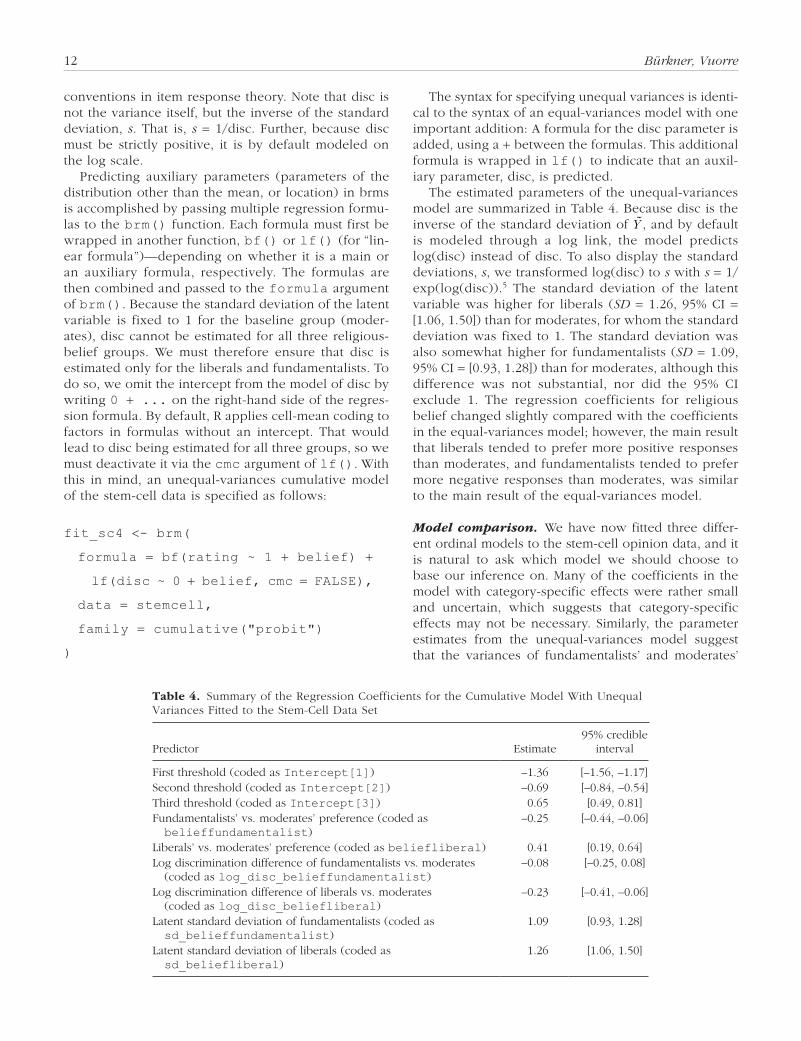
conventions in item response theory. Note that disc is not the variance itself, but the inverse of the standard deviation, s. That is, s = 1/disc. Further, because disc must be strictly positive, it is by default modeled on the log scale.

Predicting auxiliary parameters (parameters of the distribution other than the mean, or location) in brms is accomplished by passing multiple regression formu-las to the brm() function. Each formula must first be wrapped in another function, bf() or lf() (for “lin-ear formula”)—depending on whether it is a main or an auxiliary formula, respectively. The formulas are then combined and passed to the formula argument of brm(). Because the standard deviation of the latent variable is fixed to 1 for the baseline group (moder-ates), disc cannot be estimated for all three religious-belief groups. We must therefore ensure that disc is estimated only for the liberals and fundamentalists. To do so, we omit the intercept from the model of disc by writing 0 + ... on the right-hand side of the regres-sion formula. By default, R applies cell-mean coding to factors in formulas without an intercept. That would lead to disc being estimated for all three groups, so we must deactivate it via the cmc argument of lf(). With this in mind, an unequal-variances cumulative model of the stem-cell data is specified as follows:

fit_sc4 <- brm(

formula = bf(rating ~ 1 + belief) +

lf(disc ~ 0 + belief, cmc = FALSE),

data = stemcell,

family = cumulative("probit")

)

The syntax for specifying unequal variances is identi-cal to the syntax of an equal-variances model with one important addition: A formula for the disc parameter is added, using a + between the formulas. This additional formula is wrapped in lf() to indicate that an auxil-iary parameter, disc, is predicted.

The estimated parameters of the unequal-variances model are summarized in Table 4. Because disc is the inverse of the standard deviation of Y , and by default is modeled through a log link, the model predicts log(disc) instead of disc. To also display the standard deviations, s, we transformed log(disc) to s with s = 1/exp(log(disc)).5 The standard deviation of the latent variable was higher for liberals (SD = 1.26, 95% CI = [1.06, 1.50]) than for moderates, for whom the standard deviation was fixed to 1. The standard deviation was also somewhat higher for fundamentalists (SD = 1.09, 95% CI = [0.93, 1.28]) than for moderates, although this difference was not substantial, nor did the 95% CI exclude 1. The regression coefficients for religious belief changed slightly compared with the coefficients in the equal-variances model; however, the main result that liberals tended to prefer more positive responses than moderates, and fundamentalists tended to prefer more negative responses than moderates, was similar to the main result of the equal-variances model.

Model comparison. We have now fitted three differ-ent ordinal models to the stem-cell opinion data, and it is natural to ask which model we should choose to base our inference on. Many of the coefficients in the model with category-specific effects were rather small and uncertain, which suggests that category-specific effects may not be necessary. Similarly, the parameter estimates from the unequal-variances model suggest that the variances of fundamentalists’ and moderates’

Table 4. Summary of the Regression Coefficients for the Cumulative Model With Unequal Variances Fitted to the Stem-Cell Data Set

Predictor Estimate95% credible

interval

First threshold (coded as Intercept[1]) –1.36 [–1.56, –1.17]Second threshold (coded as Intercept[2]) –0.69 [–0.84, –0.54]Third threshold (coded as Intercept[3]) 0.65 [0.49, 0.81]Fundamentalists’ vs. moderates’ preference (coded as belieffundamentalist)

–0.25 [–0.44, –0.06]

Liberals’ vs. moderates’ preference (coded as beliefliberal) 0.41 [0.19, 0.64]Log discrimination difference of fundamentalists vs. moderates

(coded as log_disc_belieffundamentalist)–0.08 [–0.25, 0.08]

Log discrimination difference of liberals vs. moderates (coded as log_disc_beliefliberal)

–0.23 [–0.41, –0.06]

Latent standard deviation of fundamentalists (coded as sd_belieffundamentalist)

1.09 [0.93, 1.28]

Latent standard deviation of liberals (coded as sd_beliefliberal)

1.26 [1.06, 1.50]


opinions were quite similar, though liberals’ opinions were more variable. One formal approach to model comparison is to investigate the relative fit of computed models to the data, and one method to assess relative fit is approximate leave-one-out cross-validation (LOOCV; Vehtari, Gelman, & Gabry, 2017). LOOCV provides a score that can be interpreted in the same way as typical information criteria, such as Akaike’s information crite-rion (AIC; Akaike, 1998) or the Watanabe-Akaike infor-mation criterion (WAIC; Watanabe, 2010),6 in the sense that smaller values indicate better fit. Although a detailed exposition of this topic is beyond the scope of this article, we illustrate how to compare the relative fit of the three models we have discussed to the stem-cell data using LOOCV.

However, we also want to make sure that the dif-ferences between the equal-variances cumulative model (fit_sc1) and the adjacent-category model with category-specific effects (fit_sc2) are not due to the fact that the models belong to different classes of ordinal models. Therefore, we also fit an adjacent-category model without category-specific effects (fit_sc3); the syntax is the same as that for the model with these effects except that cs() is omitted, so we do

not show the code here. The comparison between the four ordinal models using approximate LOOCV is done via

loo( fit_sc1, fit_sc2, fit_sc3, fit_sc4)

Tables 5 and 6 display the estimated LOO informa-tion criterion (LOOIC) for each model and the differ-ences between the LOOICs for different models. As the tables show, the two cumulative models have a some-what better fit (smaller LOOIC values) than the two adjacent-category models, although the differences are not very large (not more than about 1 or 2 times the corresponding standard error). The LOOIC values for the two adjacent-category models are very similar, which implies that estimating category-specific effects does not substantially improve model fit. Similarly, the unequal-variances cumulative model has only a slightly smaller LOOIC value than the equal-variances cumula-tive model; unequal variances improve model fit slightly, but the difference is not substantial.

In the context of model selection, an LOOIC differ-ence greater than twice its corresponding standard error can be interpreted as suggesting that the model with the lower LOOIC value fits the data substantially better, at least when the number of observations is large enough.7 Although the LOOIC differences between the models are not very large, the equal- and unequal-variances cumulative models have somewhat better LOOIC values than the others, and so they might be preferred over the adjacent-category models. However, model selection—based on any metric, be it a p value, Bayes factor, or information criterion—is a controversial and complex topic, and therefore, we suggest replacing hard cutoff values with context-dependent and theory-driven reasoning. For the current example, we favor the unequal-variances cumulative model not only because of its goodness of fit (according to the LOOIC), but also because it is parsimonious and theoretically best justified.

Multiple Likert items. Although they are outside the scope of this Tutorial, we wish to briefly discuss model-ing strategies for data with multiple items per person. The extension is straightforward and can be achieved with hierarchical (multilevel) modeling.

In the stem-cell example, we have data for only one item per person. However, in many studies, the par-ticipants provide responses to multiple items. In such cases, one can fit a multilevel ordinal model that takes the items and participants into account, incorporating all information in the data into the model while con-trolling for dependencies between ratings from the same person and between ratings of the same item. For this purpose, the data need to be in long format,

Table 5. Values of the Leave-One-Out Information Criterion (LOOIC) for the Four Ordinal Models of the Stem-Cell Data

Model LOOIC SE

fit_sc1 2,040.61 31.10fit_sc2 2,042.80 31.49fit_sc3 2,043.70 30.89fit_sc4 2,039.04 31.22

Note: fit_sc1 = cumulative model with equal variances; fit_sc2 = adjacent-category model with equal variances and category-specific effects; fit_sc3 = adjacent-category model with equal variances; fit_sc4 = cumulative model with unequal variances.

Table 6. Differences Between the Leave-One-Out Information Criteria for the Four Ordinal Models of the Stem-Cell Data

Models Difference SE

fit_sc1 vs. fit_sc2 –2.20 4.94fit_sc1 vs. fit_sc3 –3.10 1.74fit_sc1 vs. fit_sc4 1.57 5.16fit_sc2 vs. fit_sc3 –0.90 6.07fit_sc2 vs. fit_sc4 3.76 1.52fit_sc3 vs. fit_sc4 4.66 6.34

Note: For each pair of models, the table shows the difference between the information criterion for the model listed first and the information criterion for the model listed second (first model – second model). For a description of the four models, see the footnote to Table 5.

14 Bürkner, Vuorre

such that each row gives a single rating and the col-umns show the values of ratings and identifiers for the participants and items. If opinion about funding stem-cell research had been measured with multiple items, we might call the identifier columns person and item, respectively. Then, we could write the model formula as follows:

rating ~ 1 + belief + (1|person) + (1|item)

The notation (1|<group>) (e.g., (1|person) or (1|item)) implies that the intercept (1) varies over the levels of the grouping factor (<group>). Ordinal mod-els have multiple intercepts (recall that intercepts are called thresholds in ordinal models), and (1|<group>) allows these thresholds to vary by the same amount across levels of the grouping factor. To model threshold-specific variances, we would write (cs(1)|<group>). For instance, if we want all thresholds to vary differently across items so that each item receives its own set of thresholds, we could add (cs(1)|item) to the model formula.

Summary. In summary, we have illustrated the use of cumulative models (with and without unequal variances) and adjacent-category models (with and without category-specific effects) in the context of a Likert-item response variable. We have illustrated how to fit these four models to data using concise R syntax, enabled by the brm() function, and how to summarize, interpret, and visualize the model’s estimated parameters. Paired with effective visualization (see Fig. 2), the models’ results are readily interpretable and rich in information because of their fully Bayesian estimation. For the data set we used to illustrate the models, we found that cate-gory-specific effects did not meaningfully improve model fit, and that the cumulative models were a better fit than the adjacent-category models. Further, there was a small improvement in model fit in the unequal-variances cumu-lative model relative to the equal-variances cumulative model.

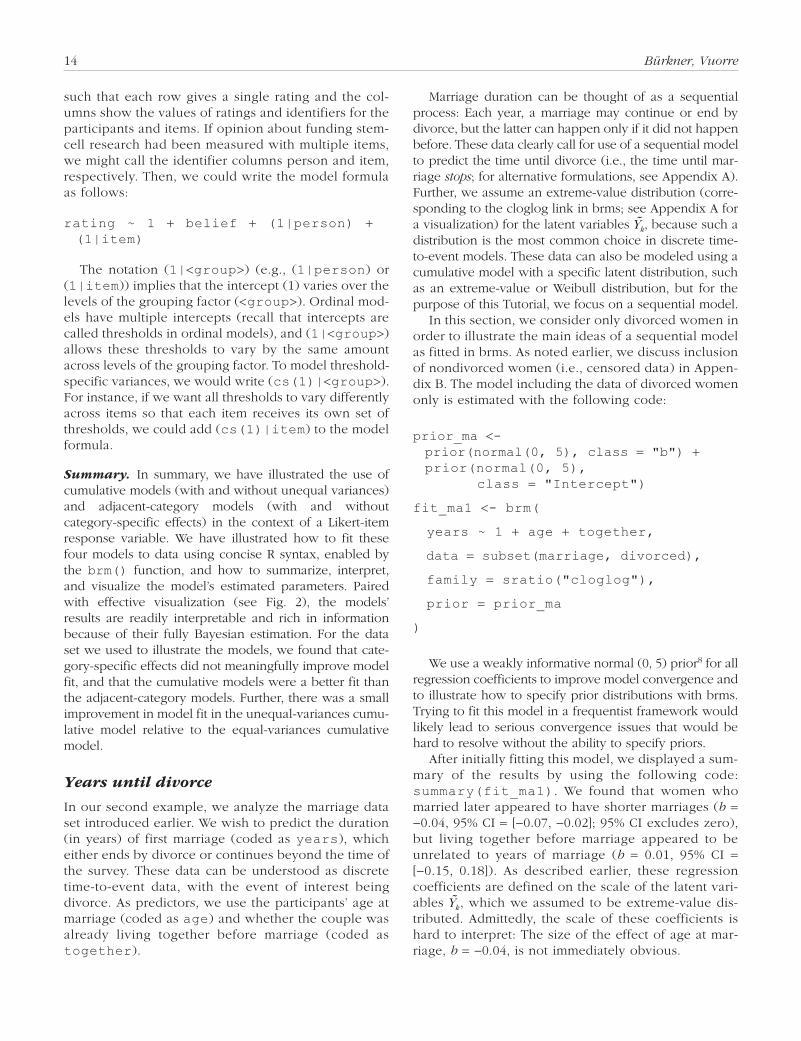
Years until divorce

In our second example, we analyze the marriage data set introduced earlier. We wish to predict the duration (in years) of first marriage (coded as years), which either ends by divorce or continues beyond the time of the survey. These data can be understood as discrete time-to-event data, with the event of interest being divorce. As predictors, we use the participants’ age at marriage (coded as age) and whether the couple was already living together before marriage (coded as together).

Marriage duration can be thought of as a sequential process: Each year, a marriage may continue or end by divorce, but the latter can happen only if it did not happen before. These data clearly call for use of a sequential model to predict the time until divorce (i.e., the time until mar-riage stops; for alternative formu lations, see Appendix A). Further, we assume an extreme-value distribution (corre-sponding to the cloglog link in brms; see Appendix A for a visualization) for the latent variables Yk, because such a distribution is the most common choice in discrete time-to-event models. These data can also be modeled using a cumulative model with a specific latent distribution, such as an extreme-value or Weibull distribution, but for the purpose of this Tutorial, we focus on a sequential model.

In this section, we consider only divorced women in order to illustrate the main ideas of a sequential model as fitted in brms. As noted earlier, we discuss inclusion of nondivorced women (i.e., censored data) in Appen-dix B. The model including the data of divorced women only is estimated with the following code:

prior_ma <- prior(normal(0, 5), class = "b") + prior(normal(0, 5), class = "Intercept")

fit_ma1 <- brm(

years ~ 1 + age + together,

data = subset(marriage, divorced),

family = sratio("cloglog"),

prior = prior_ma

)

We use a weakly informative normal (0, 5) prior8 for all regression coefficients to improve model convergence and to illustrate how to specify prior distributions with brms. Trying to fit this model in a frequentist framework would likely lead to serious convergence issues that would be hard to resolve without the ability to specify priors.

After initially fitting this model, we displayed a sum-mary of the results by using the following code: summary(fit_ma1). We found that women who married later appeared to have shorter marriages (b = −0.04, 95% CI = [−0.07, −0.02]; 95% CI excludes zero), but living together before marriage appeared to be unrelated to years of marriage (b = 0.01, 95% CI = [−0.15, 0.18]). As described earlier, these regression coefficients are defined on the scale of the latent vari-ables Yk, which we assumed to be extreme-value dis-tributed. Admittedly, the scale of these coefficients is hard to interpret: The size of the effect of age at mar-riage, b = −0.04, is not immediately obvious.


For this reason, we recommend always plotting the results, for instance, with marginal_effects(fit_ma1). In this case, years of marriage has a natural metric interpretation. As shown in the left panel of Figure 3, between the minimum and maximum age at marriage (12 and 43 years, respectively), the model predicts a 3.95-year difference in the time until divorce. In contrast, according to this model, it appears to make little difference whether a couple was living together before marriage (see the right panel of Fig. 3).

However, this model omits an important detail in the data: We included only those women who actually got divorced during the study, and excluded those who were still married at the end of the study. In the context of time-to-event analysis, this is called (right) censoring, because divorce might happen later on in time. Both excluding nondivorced women altogether (as we did in the preceding analysis) and falsely treating them as being divorced right at the end of the study may lead to bias of unknown direction and magnitude in the results.

For these reasons, it is important to find a way to incorporate censored data into the model. In the stan-dard version of the sequential model, each observation must have an associated outcome category. However, for censored data, the outcome category was unob-served. Expanding the standard sequential model to include such data requires a little bit of extra work, to which we turn in Appendix B.

Conclusion

In this Tutorial, we have introduced three important classes of ordinal models: cumulative, sequential, and adjacent-category models. We have applied these mod-els to real-world data sets that come from different psychological fields and that can answer different

research questions. The models are formally derived from their underlying assumptions in Appendix A, but we do not demonstrate (e.g., via simulations) that using ordinal models for ordinal data is superior to other approaches, such as linear regression, because this topic has already been sufficiently covered elsewhere (Liddell & Kruschke, 2018). Nevertheless, we briefly discuss some possible objections to using ordinal mod-els and provide counterarguments.

Objections and counterarguments

Although we have highlighted the theoretical justifica-tion, and practical ease, of applying ordinal models to ordinal data, some readers might still object to using these models. For example, one possible objection is that the results of ordinal models are more difficult to interpret and communicate than the results of corre-sponding linear regression models. However, the main complexity of ordinal models, relative to linear regres-sion models, is in the threshold parameters, which (like intercept parameters in linear regression) are rarely the main target of inference. Usually, researchers are more interested in the predictors, and the predictors in ordi-nal models can be interpreted in the same way as ordi-nary predictors in linear regression models (though they are on the latent metric scale). Furthermore, the helper functions in brms make it easy to calculate (see ?fitted.brmsfit) and visualize (see ?marginal_effects.brmsfit) a model’s fitted values (i.e., the predicted proportion of each response category for a given set of predictor values).

Another possible objection is that sometimes one’s substantial conclusions do not strongly depend on whether an ordinal or a linear regression model was used. We wish to point out, though, that even though the actionable conclusions may be similar, a linear

4

5

6

7

8

9

6.25

6.50

6.75

7.00

7.25

20 30 No YesAge Together

Year

s Un

til D

ivor

ce

Year

s Un

til D

ivor

ce

Fig. 3. Marginal effects of a woman’s age at marriage (left) and living together before marriage (right) on the number of years of marriage until divorce, with censored data excluded (data from Centers for Disease Control and Prevention, n.d.). The shaded area in the left panel represents the 95% credible intervals around the estimates.

16 Bürkner, Vuorre

model will have a lower predictive utility by virtue of assuming a theoretically incorrect outcome distribution. Perhaps more important is the fact that using linear models for ordinal data can lead to effect-size estimates that are distorted in size or certainty, and this problem is not solved by averaging data for multiple ordinal items (Liddell & Kruschke, 2018).

Software options

We have advocated and illustrated the implementation of ordinal models using the brms package in the R statistical computing environment. The main reason for our choice of these software options is that they are completely free and open source. Therefore, they are available to anyone, without any licensing fees. In addi-tion, many computational and statistical procedures are implemented in R before they are available in other (commercial) software packages. Further, we believe that the wide variety of models that can be computed through the concise and consistent syntax of brms is beneficial to any modeling endeavor (Bürkner, 2017, 2018).

Nevertheless, users may wish to implement ordinal models within their preferred statistical packages. Explaining how to conduct ordinal regressions using other software is outside the scope of this Tutorial. Useful references include Heck, Thomas, and Tabata (2013) for IBM SPSS; Bender and Benner (2000) for SAS and S-Plus; and Long, Long, and Freese (2006) for Stata.

Choosing between ordinal models

Equipped with the knowledge about the three classes of ordinal models, researchers might still find it difficult to decide which type of model best fits their research question and data. It is impossible to describe in advance which class would best fit each situation, but here we briefly describe some useful rules of thumb for deciding among the models we have discussed.

From a theoretical perspective, if the response under study can be understood as the categorization of a latent continuous construct, we recommend using a cumulative model. The categorization interpretation is natural for many Likert-item data sets, in which ordered verbal (or numeri-cal) labels are used to obtain discrete responses about a continuous psychological variable. Cumulative models are also computationally less intensive than the other types of models, and therefore faster to estimate. If unequal vari-ances are theoretically possible—and they usually are—we recommend incorporating them into the model; ignoring them may lead to increased false alarm rates and inaccurate parameter estimates (Liddell & Kruschke, 2018). Further, we think that (differences in) variances, although often overlooked, can themselves be theoretically interesting and therefore should be modeled.

If the response under study can be understood as the result of a sequential process, such that a higher response category is possible only after all lower cat-egories are achieved, we recommend using a sequential model. Sequential models are therefore especially use-ful, for example, for discrete time-to-event data. How-ever, deciding between a categorization and a sequential process may not always be straightforward; in ambigu-ous situations, estimating both types of models may be a reasonable strategy.

If category-specific effects are of interest, we recom-mend using a sequential or adjacent-category model. It is useful to model category-specific effects when there is reason to expect that a predictor might affect the response variable differently at different levels of the response variable. Finally, we suggest that if one wishes to model ordinal responses, it is important to use an ordinal model of any type instead of falsely assuming metric or nominal responses.

Appendix A: Derivations of the Three Classes of Ordinal Models

In this appendix, we derive and discuss in more detail the classes of ordinal models illustrated in the main text. Throughout, we assume that the data consist of a total of N values of the ordinal response variable Y with K + 1 categories from 1 to K + 1.

Cumulative model

The cumulative model, sometimes also called the graded response model (Samejima, 1997), assumes that the observed ordinal variable Y originates from the categorization of a latent (i.e., not observable) continu-ous variable Y . That is, there are latent thresholds τk (1≤ k ≤ K) that partition the values of Y into the K + 1 observable, ordered categories of Y. More formally, this model can be written as follows:

Y k Yk k= ⇔ < ≤τ τ–1 (A1)

for −∞ = τ0 < τ1 < . . . < τk < τk+1 = ¥. We write τ = (τ1, . . . , τk) for the vector of the thresholds. As explained earlier, it may not be valid to use linear regression on Y, because the differences between its categories are not known. However, linear regression is applicable to Y . Using η to symbolize the predictor term leads to

Y ,= +η ε (A2)

where ε is the random error of the regression with E(ε) = 0. As there are multiple observations in the data, it would be more explicit to write Yn, ηn, and εn in all equations. However, we omit the index n for simplicity,


because it is not required to understand the ideas and derivations of the models.

In the simplest case, η is a linear predictor of the form η = Xb = x1b1 + x2b2 + . . . + xmbm, with m predic-tor variables X = (x1, . . . , xm) and corresponding regression coefficients b = (b1, . . . , bm) (without an intercept). The predictor term η may also take more complex forms—for instance, multilevel structures or nonlinear relationships. However, for the understanding of ordinal models, the exact form of η is irrelevant, and we can assume it to be linear for now.

To complete Model A2, the distribution F of ε has to be specified. We might use the normal distribution because it is the default in linear regression, but alter-natives such as the logistic distribution are also possi-ble. Depending on the choice of F, the final model for Y and also for Y will vary. At this point, we do not want to narrow down our modeling flexibility and therefore just assume that εn is distributed according to F:

Pr( ) .ε ≤ = ( )z F z (A3)

Combining the assumptions in Equations A1, A2, and A3 leads to

Pr Pr Pr

Pr

( | ) ( | ) ( )

( ) ( ).

Y k Y

Fk k

k k

≤ = ≤ = + ≤= ≤ =

η τ η η ε τε τ − η τ − η

(A4)

The notation |η in the first two terms of Equation A4 means that the probabilities will depend on the value of the predictor term η. Equation A4 says that the prob-ability of Y being in category k or less (depending on η) is equal to the value of the distribution F at the point τ ηk − . In this context, F is also called a response func-tion or processing function. In this Tutorial, we use the terms distribution and response function interchange-ably when talking about F. In the case of the cumulative model, F models the probability of the binary outcome Y ≤ k against Y > k (hence the name “cumulative” model).

The probabilities Pr(Y ≤ k|η), which are of primary interest, can be easily derived from Equation A4, because

Pr Pr Pr 1

1

( | ) ( | ) ( | )

( ) ( ).

Y k Y k Y k

F Fk k

= = ≤ ≤=

η η − − ητ − η − τ − η−

(A5)

The cumulative model as formulated in Equation A5 assumes that the predictor term η is constant across the response categories. It is plausible that a predictor may have, for instance, a higher impact on the lower categories of an item than on its higher categories. Thus, we could write ηk to indicate that the predictor

term may vary across categories. For instance, if we had four response categories and two predictor variables x1 and x2, with ηk = b1k x1 + b2k x2, we would have six (3 × 2) regression parameters instead of just two. Admit-tedly, the fully category-specific model is not very par-simonious. Further, estimating regression parameters as varying across response categories in the cumulative model is not always possible, because it may result in negative probabilities (Tutz, 2000; Van Der Ark, 2001). This can be seen from Equation A5 as follows. If cate-gory-specific effects are assumed, ηk may be different from ηk+1 and thus

F Fk k k k k k k k( ) ( ) .τ − η − τ − η τ − η τ − η+ + + +< <1 1 1 1 if0 (A6)

Accordingly, we have to assume η to be constant across categories when using the cumulative model. The threshold parameters τk , however, are estimated for each category separately, which leads to a total of K threshold parameters. This does not mean that it is always necessary to estimate so many of them: We can assume that the distance between two adjacent thresh-olds τk and τk+1 is the same for all thresholds, which leads to

τ τ δk k= + ( )1 1– . (A7)

Accordingly, only τ1 and δ have to be estimated. Parameterizations of the form of Equation A7 are often referred to as rating scale models (Andersen, 1977; Andrich, 1978a, 1978b) and can be used not only in cumulative models, but also in many item response theory and regression models. When several items that each have several categories are administered, a rating scale model leads to a remarkable reduction in the number of threshold parameters. Consider an example with seven response categories. Under Equation A5, there are six threshold parameters, but using Equation A7 reduces this number to only two. The difference is even larger when there are more categories. (More details about different parameterizations of the cumula-tive model can be found in, e.g., Samejima, 1969, 1995, 1997). Note that in regression models, the threshold parameters are usually of subordinate, interest as they serve only as intercept parameters. For this reason, restrictions to τk, such as Equation A7, are rarely applied in regression models.

The derivation and formulation of the general cumu-lative model presented thus far is from Tutz (2000). The cumulative model was first proposed by Walker and Duncan (1967), but only in the special case in which F is the standard logistic distribution, that is, when

18 Bürkner, Vuorre

F xx

x( ) =

+( )

( )

exp

exp1 (A8)

(see Fig. A1, green line). This special model was later called the proportional odds model by McCullagh (1980), and it is the most frequently used version of the cumulative model (McCullagh, 1980; Van Der Ark, 2001). In many articles, the proportional odds model is presented as if it were the only version of the cumu-lative model, and the possibility of using response func-tions other than the logistic distribution is ignored (Ananth & Kleinbaum, 1997; Guisan & Harrell, 2000; Van Der Ark, 2001), thus hindering general understand-ing of the cumulative model’s ideas and assumptions.

The name proportional odds model stems from the fact that under this model, the odds ratio of Pr( | )Y k≤ 1 η against Pr( | )Y k≤ 2 η for any 1 ≤ k1 and k2 ≤ K is indepen-dent of η and depends only on the distance between the thresholds τ k1

and τ k2:

Pr Pr

Pr Prexp

( | ) / ( | )

( | ) / ( | )( ).

Y k Y k

Y k Y k k k

≤ >≤ >

=1 1

2 21 2

η ηη η

−τ τ (A9)

Equation A9 is often called the proportional odds assumption.9

Another version of the cumulative model, the pro-portional hazards model, is derived when F is the extreme-value distribution (Cox, 1972; McCullagh, 1980):

F x x( ) = ( )( )1 exp exp– – (A10)

(see Fig. A1, red line). This model was originally invented in the context of survival analysis for discrete points in time. It is also possible to use the standard normal distribution,

F x x e dzx

z

( )= ( )=−∞

−

∫ ,Φπ

1

2

2

2 (A11)

as a response function (see Fig. A1, blue line). Of course, one can use other distributions for F as well.

Following the conventions of generalized linear models, statisticians often refer to the distribution using the name of the inverse distribution function F –1, called the link function, instead of the name of distribution function F itself. The link functions associated with the logistic, normal, and extreme-value distributions are called logit, probit, and cloglog links, respectively. Applying cumulative models with different response functions to the same data will often lead to similar estimates of the parameters τ and b, as well as to simi-lar model fits (McCullagh, 1980), so the distribution chosen usually has only a minor impact on the results.

The derivation of the cumulative model we have pre-sented here demonstrates that this model is especially

appealing when the ordinal data Y can be understood as a categorization of a continuous latent variable Y , because the thresholds τk have an intuitive meaning in this case. However, the cumulative model is also appli-cable when this assumption seems unreasonable. In particular, the regression parameters b (and inferences about them) remain interpretable in the same way even when Y cannot readily be understood as a categoriza-tion of a continuous latent variable Y (McCullagh, 1980).

Sequential model

The dependent variable Y in this model results from a counting process and is truly ordinal in the sense that in order to achieve a category k, one must first achieve all lower categories 1 through k – 1. The gen-eral sequential model proposed by Tutz (1990), which is the version we present here, explicitly incorporates this structure into its assumptions (see also Tutz, 2000). For every category k ∈ {1, . . . , K}, there is a latent continuous variable Y determining the transi-tion to the k + 1th category. The variables Y may have different meanings depending on the research ques-tion. We assume that Y depends on the predictor term η and error εk :

Yk k .= +η ε (A12)

As in the cumulative model, εk has a mean of zero and is distributed according to F:

Pr( ) ( ).εk z F z≤ = (A13)

The sequential process itself is understood as fol-lows: If Y1 does not surpass the first threshold, τ1, that is, if Y1 ≤ τ1, the process stops, and the result is Y = 1. If Y1 > τ1 , at least category 2 is achieved (i.e., Y > 1), and the process continues. Then, if Y2 does not surpass

.00

.25

.50

.75

1.00

−4 −2 0 2 4x

Prob

abili

ty

Distribution

Extreme ValueLogisticNormal

Fig. A1. Illustration of various possible choices for the distribution function F in ordinal models.


threshold τ2 , the process stops with the result Y = 2. Otherwise, the process continues with Y > 2. More generally, given categories k ∈ {1, . . . , K}, the process stops with the result Y = k, when category k is achieved but Yk fails to surpass the kth threshold. This event can be written as

Y k Y k= ≥| . (A14)

Combining Equations A12, A13, and A14 leads to

Pr Pr

Pr

Pr

( | , ) ( | )

( )

( )

(

Y k Y k Y

F

k k

k k

k k

k

= ≥ = ≤= + ≤= ≤=

η τ ηη ε τε τ − ητ −

ηη). (A15)

Equation A15 can equivalently be expressed by

Pr( | )Y k F Fkj

k

j( ) ( ( )).= ==

−

∏η τ −η − τ −η1

1

1 (A16)

Because of its derivation, this model is sometimes also called the stopping model. A related sequential model was proposed by Verhelst, Glas, and De Vries (1997), who used item response theory notation and focused on the logistic response function only. Instead of mod-eling the probability of the sequential process stopping at category k (Equation A15), they suggested modeling the probability of the sequential process continuing beyond category k. In our notation, this can generally be written as

Pr 1( , ) ( )|Y k Y k F k≥ ≥ =− η η− τ (A17)

or, equivalently,

Pr( | )Y k F Fk j

k

j( ( )) ( ).= = −=

−∏η τ −η τ −η11

1 (A18)

In the following, we call Equation A16 the SMS (short for “sequential model with stopping parameterization”) and Equation A18 the SMC (short for “sequential model with continuation parameterization”). When F is sym-metric, the SMS and SMC are identical, because the relation F(–x) = 1 – F(x) holds for symmetric distribu-tions. Both the normal and the logistic distributions (Equations A11 and A8, respectively) are symmetric. Thus, there is only one sequential model for these distributions. The sequential model combined with the logistic distribution is often called the continuation ratio model (Fienberg, 1980/2007). An example of an asymmetric response function is the extreme-value dis-tribution (Equation A10). In this case, the SMS and SMC are different from each other, but, surprisingly, the SMS

is equivalent to the cumulative model (Läärä & Matthews, 1985). That is, the proportional hazards model (Cox, 1972) arises from assumptions of both cumulative and sequential models.

Despite their obvious relation to each other, the SMS and SMC are discussed independently in two adjacent chapters in van der Linden and Hambleton’s (1997) handbook (see also Tutz, 1997; Verhelst et al., 1997). Such treatment gives the impression that they are unrelated models and therefore could lead to some confusion. This underlines the need for consistent wording and notation of ordinal models, in order to facilitate researchers’ understanding and practical use of them.

The regression parameters b in the sequential model may vary across categories. Although estimating cate-gory-specific regression parameters is usually less of an issue for the sequential model than for the cumula-tive model (Tutz, 1990, 2000), a sequential model may still be unattractive because of the high number of parameters. Of course, restrictions to the thresholds τk, such as the rating scale model (Equation A7), are also applicable. Although the sequential model is par-ticularly appealing when Y can be understood as the result of a sequential process, it is applicable to all ordinal dependent variables regardless of their origin.

Adjacent-category model

The adjacent-category model is somewhat different from the cumulative and sequential models because, in our opinion, it has no satisfying theoretical derivation. For this reason, we discuss the ideas behind the adja-cent-category model after introducing its formulas. The adjacent-category model is defined as follows (Agresti, 1984, 2010):

Pr 1( , , ) ( ).|Y k Y k k F k= ∈ +{ } =η τ − η (A19)

This model describes the probability that category k, rather than category k + 1, is achieved. This can equiva-lently be written as

Pr |Y kF F

j

k

j j k

K

j

r

K

j

( ( )) ( )=( )=

− − −=

−

=

=

+

∏ ∏∑

ητ η τ η

1

1

1

1

1

==

−

=∏ ∏− − −1

11

r

j j r

K

jF F( ( )) ( ),

τ η τ η (A20)

with

j

jj K

K

jF F= = +∏ ∏− − = −

1

0

1

1 1( ( )) ( ) :τ η τ η = (A21)

for notational convenience. To our knowledge, the adjacent-category model has almost solely been applied

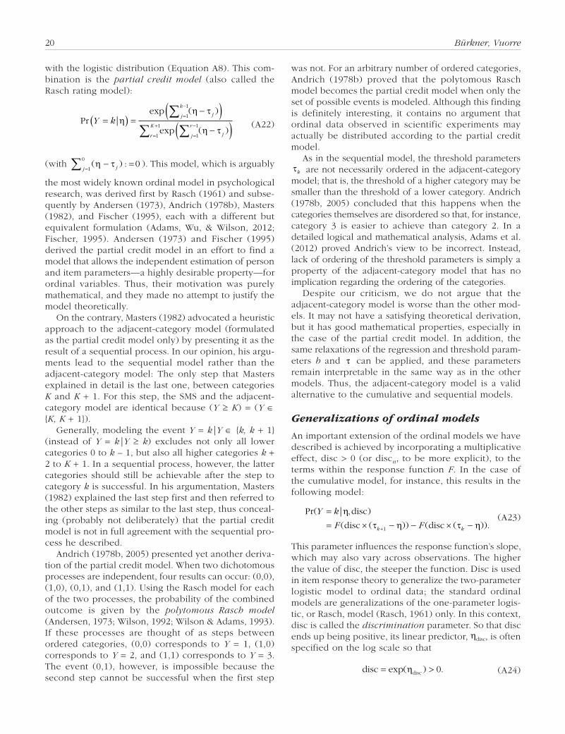
20 Bürkner, Vuorre

with the logistic distribution (Equation A8). This com-bination is the partial credit model (also called the Rasch rating model):

Pr |exp

expY k

j

k

j

r

K

j

r

j

=( ) =−( )−( )

=

−

=

+

=

−

∑∑ ∑

ηη τ

η τ

1

1

1

1

1

1

( )

( ) (A22)

(with ( ) :η τ− ==∑ jj 1

00 ). This model, which is arguably

the most widely known ordinal model in psychological research, was derived first by Rasch (1961) and subse-quently by Andersen (1973), Andrich (1978b), Masters (1982), and Fischer (1995), each with a different but equivalent formulation (Adams, Wu, & Wilson, 2012; Fischer, 1995). Andersen (1973) and Fischer (1995) derived the partial credit model in an effort to find a model that allows the independent estimation of person and item parameters—a highly desirable property—for ordinal variables. Thus, their motivation was purely mathematical, and they made no attempt to justify the model theoretically.

On the contrary, Masters (1982) advocated a heuristic approach to the adjacent-category model (formulated as the partial credit model only) by presenting it as the result of a sequential process. In our opinion, his argu-ments lead to the sequential model rather than the adjacent-category model: The only step that Masters explained in detail is the last one, between categories K and K + 1. For this step, the SMS and the adjacent-category model are identical because (Y ≥ K) = (Y ∈ {K, K + 1}).

Generally, modeling the event Y = k|Y ∈ {k, k + 1} (instead of Y = k|Y ≥ k) excludes not only all lower categories 0 to k – 1, but also all higher categories k + 2 to K + 1. In a sequential process, however, the latter categories should still be achievable after the step to category k is successful. In his argumentation, Masters (1982) explained the last step first and then referred to the other steps as similar to the last step, thus conceal-ing (probably not deliberately) that the partial credit model is not in full agreement with the sequential pro-cess he described.

Andrich (1978b, 2005) presented yet another deriva-tion of the partial credit model. When two dichotomous processes are independent, four results can occur: (0,0), (1,0), (0,1), and (1,1). Using the Rasch model for each of the two processes, the probability of the combined outcome is given by the polytomous Rasch model (Andersen, 1973; Wilson, 1992; Wilson & Adams, 1993). If these processes are thought of as steps between ordered categories, (0,0) corresponds to Y = 1, (1,0) corresponds to Y = 2, and (1,1) corresponds to Y = 3. The event (0,1), however, is impossible because the second step cannot be successful when the first step

was not. For an arbitrary number of ordered categories, Andrich (1978b) proved that the polytomous Rasch model becomes the partial credit model when only the set of possible events is modeled. Although this finding is definitely interesting, it contains no argument that ordinal data observed in scientific experiments may actually be distributed according to the partial credit model.

As in the sequential model, the threshold parameters τk are not necessarily ordered in the adjacent-category model; that is, the threshold of a higher category may be smaller than the threshold of a lower category. Andrich (1978b, 2005) concluded that this happens when the categories themselves are disordered so that, for instance, category 3 is easier to achieve than category 2. In a detailed logical and mathematical analysis, Adams et al. (2012) proved Andrich’s view to be incorrect. Instead, lack of ordering of the threshold parameters is simply a property of the adjacent-category model that has no implication regarding the ordering of the categories.

Despite our criticism, we do not argue that the adjacent-category model is worse than the other mod-els. It may not have a satisfying theoretical derivation, but it has good mathematical properties, especially in the case of the partial credit model. In addition, the same relaxations of the regression and threshold param-eters b and τ can be applied, and these parameters remain interpretable in the same way as in the other models. Thus, the adjacent-category model is a valid alternative to the cumulative and sequential models.


An important extension of the ordinal models we have described is achieved by incorporating a multiplicative effect, disc > 0 (or discn, to be more explicit), to the terms within the response function F. In the case of the cumulative model, for instance, this results in the following model:

Pr disc

disc disc1

( | , )

( ( )) ( ( )).

Y k

F Fk k

== × ×+

ητ − η − τ − η

(A23)

This parameter influences the response function’s slope, which may also vary across observations. The higher the value of disc, the steeper the function. Disc is used in item response theory to generalize the two-parameter logistic model to ordinal data; the standard ordinal models are generalizations of the one-parameter logis-tic, or Rasch, model (Rasch, 1961) only. In this context, disc is called the discrimination parameter. So that disc ends up being positive, its linear predictor, ηdisc, is often specified on the log scale so that

disc exp disc= >( ) .η 0 (A24)


One may also use the inverse, s = 1/disc, to model the standard deviation of the latent variables, as explained in the main text’s section on modeling opinions about funding stem-cell research.

Appendix B: Modeling the Number of Years Until Divorce

In this appendix, we continue with the discussion of using a sequential model to predict the number of years of marriage until divorce. In particular, we show how to incorporate censored data into the sequential model we described earlier for analyzing the marriage-duration data from the U.S. National Survey of Family Growth (Centers for Disease Control and Prevention, n.d.). This extension is necessary because—quite fortunately—not all marriages ended with divorce at the end of the study’s observation period.

In the field of time-to-event analysis, the hazard rate plays a crucial role (Cox, 1972). For discrete time-to-event data, the hazard rate at time t, h(t), is simply the probability that the event occurs at time t given that the event did not occur up through time t – 1. In our notation, the hazard rate at time t can be written as

h t F t( ) ( ).= τ − η (B1)

Comparing this with Equation A15, we see that the stop-ping sequential model is simply the product of h(t) and 1 – h(t) terms for varying values of t. Each of these terms defines the event probability of a Bernoulli variable (0 = still married beyond time t; 1 = divorced at time t), so the sequential model can be understood as a sequence of conditionally independent Bernoulli trials. Accordingly, we can equivalently write the sequential model in terms of binary regression10 by expanding each of the outcome variables into a sequence of 0s and 1s.11 More precisely, for each couple, we create a single row for each year of marriage, entering the outcome variable as 1 if the couple divorced in that year and as 0 otherwise. The expanded data are exemplified in Table B1.

In the expanded data set, discrete_time indi-cates the length of the marriage (in years) for each row of the data. It is treated as a factor so that, when it is included in a model formula in brms, its coefficients will represent the threshold parameters. This can be done in at least two ways. First, we could write ... ~ 0 + discrete_time + ... , in which case the coefficients can immediately be interpreted as thresholds. Second, we could write ... ~ 1 + discrete_time + ... , so that the intercept is the first threshold, and the K −1 coefficients of discrete_time represent dif-ferences between the respective other thresholds and the

Table B1. Illustration of the Marriage Data From the 2013–2015 U.S. National Survey of Family Growth (Centers for Disease Control and Prevention, n.d.) When Expanded for Use in Binary Regression

Couple (coded as ID)

Couple lived together before

marriage? (coded as together)

Woman’s age at marriage (coded as age)

Divorced at time of survey

(coded as divorced)

Year of marriage (coded as

discrete_time)

1 Yes 19 0 11 Yes 19 0 21 Yes 19 0 31 Yes 19 0 41 Yes 19 0 51 Yes 19 0 61 Yes 19 0 71 Yes 19 0 81 Yes 19 1 92 Yes 22 0 12 Yes 22 0 22 Yes 22 0 32 Yes 22 0 42 Yes 22 0 52 Yes 22 0 62 Yes 22 0 72 Yes 22 0 82 Yes 22 0 9

Note: The divorce variable has a value of 1 if the couple divorced during the year indicated and 0 otherwise.

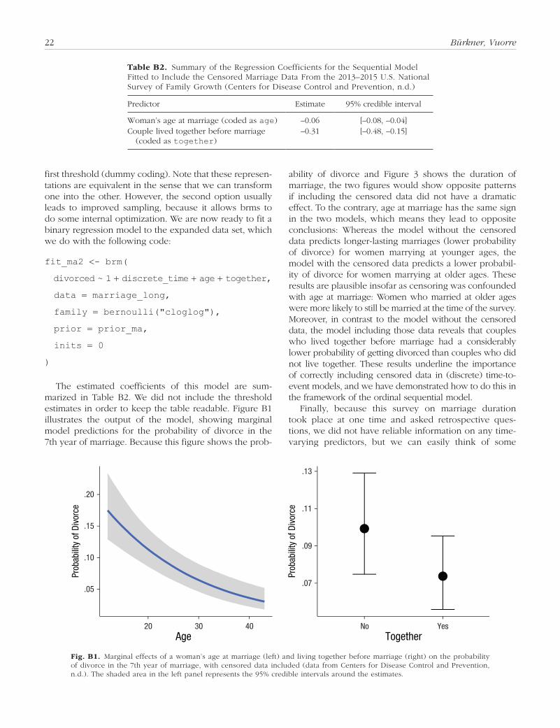
22 Bürkner, Vuorre

first threshold (dummy coding). Note that these represen-tations are equivalent in the sense that we can transform one into the other. However, the second option usually leads to improved sampling, because it allows brms to do some internal optimization. We are now ready to fit a binary regression model to the expanded data set, which we do with the following code:

fit_ma2 <- brm(

divorced ~ 1 + discrete_time + age + together,

data = marriage_long,

family = bernoulli("cloglog"),

prior = prior_ma,

inits = 0

)

The estimated coefficients of this model are sum-marized in Table B2. We did not include the threshold estimates in order to keep the table readable. Figure B1 illustrates the output of the model, showing marginal model predictions for the probability of divorce in the 7th year of marriage. Because this figure shows the prob-

ability of divorce and Figure 3 shows the duration of marriage, the two figures would show opposite patterns if including the censored data did not have a dramatic effect. To the contrary, age at marriage has the same sign in the two models, which means they lead to opposite conclusions: Whereas the model without the censored data predicts longer-lasting marriages (lower probability of divorce) for women marrying at younger ages, the model with the censored data predicts a lower probabil-ity of divorce for women marrying at older ages. These results are plausible insofar as censoring was confounded with age at marriage: Women who married at older ages were more likely to still be married at the time of the survey. Moreover, in contrast to the model without the censored data, the model including those data reveals that couples who lived together before marriage had a considerably lower probability of getting divorced than couples who did not live together. These results underline the importance of correctly including censored data in (discrete) time-to-event models, and we have demonstrated how to do this in the framework of the ordinal sequential model.

Finally, because this survey on marriage duration took place at one time and asked retrospective ques-tions, we did not have reliable information on any time-varying predictors, but we can easily think of some

Table B2. Summary of the Regression Coefficients for the Sequential Model Fitted to Include the Censored Marriage Data From the 2013–2015 U.S. National Survey of Family Growth (Centers for Disease Control and Prevention, n.d.)

Predictor Estimate 95% credible interval

Woman’s age at marriage (coded as age) –0.06 [–0.08, –0.04]Couple lived together before marriage

(coded as together)–0.31 [–0.48, –0.15]

.05

.10

.15

.20

.07

.09

.11

.13

20 30 40 No YesAge Together

Prob

abili

ty o

f Div

orce

Prob

abili

ty o

f Div

orce

Fig. B1. Marginal effects of a woman’s age at marriage (left) and living together before marriage (right) on the probability of divorce in the 7th year of marriage, with censored data included (data from Centers for Disease Control and Prevention, n.d.). The shaded area in the left panel represents the 95% credible intervals around the estimates.


potential ones. For instance, the probability of divorce may change over the duration of marriage as a couple’s socioeconomic status changes. Such time-varying pre-dictors cannot be modeled in the standard sequential model, because all information about a single marriage process has to be stored within the same row in the data set. Fortunately, time-varying predictors can easily be added to the expanded data set shown in Table B2 and then treated in the same way as other predictors in the binary regression model.

Action Editor

Pamela Davis-Kean served as action editor for this article.

Author Contributions

P.-C. Bürkner generated the idea for the manuscript and wrote the first draft of the theoretical part of the manuscript. The two authors jointly wrote the first draft of the practical part of the manuscript. Both authors critically edited the entire draft and approved the final submitted version of the manuscript.

ORCID iDs

Paul-Christian Bürkner https://orcid.org/0000-0001-57 65-8995Matti Vuorre https://orcid.org/0000-0001-5052-066X

Declaration of Conflicting Interests

The author(s) declared that there were no conflicts of interest with respect to the authorship or the publication of this article.

Open Practices

All data and materials have been made publicly available via the Open Science Framework and can be accessed at https://osf.io/cu8jv/. The complete Open Practices Disclosure for this article can be found at http://journals.sagepub.com/doi/suppl/10.1177/2515245918823199. This article has received badges for Open Data and Open Materials. More information about the Open Practices badges can be found at http://www .psychologicalscience.org/publications/badges.

Notes

1. Note that we reversed the numerical order of the original ratings to allow a more straightforward interpretation in which greater values map to more positive constructs.2. In linear regression, describing the response as normally dis-tributed around the linear predictor (i.e., the regression line) is equivalent to describing the errors as normally distributed around zero. The same principle applies to the latent variables in an ordinal model.3. A brief introduction to R basics can be found at http://blog .efpsa.org/2016/12/05/introduction-to-data-analysis-using-r/ (Vuorre, 2016). For a comprehensive, book-length tutorial, we recommend Wickham and Grolemund (2016).

4. The assumption of equal variances of residuals can be relaxed in linear regression models as well. However, with ordinal models, equal and unequal variances refer to the latent variable Y and not to the manifest variable Y (Liddell & Kruschke, 2018).5. Note that this transformation must be done on the posterior samples of disc, not on its posterior summary. The R code to transform disc to s is available at the Open Science Framework (https://osf.io/cu8jv/). Also note that in the summary output of brms, coefficients for the log of discrimination just have the prefix disc_, although they are in fact on the log scale.6. The AIC and WAIC methods can be interpreted as approxi-mations of LOOCV.7. LOOIC values and their differences are approximately nor-mally distributed. Hence, when a model is based on enough observations, one may construct a frequentist confidence inter-val around the estimate. For instance, a 95% confidence interval around ΔLOOIC can be constructed via the following calcula-tions: ΔLOOIC – 1.96 × SE(ΔLOO) for the lower bound and ΔLOOIC + 1.96 × SE(ΔLOO) for the upper bound.8. This prior is weakly informative for the present model and variable scales. However, it may be more informative for other models or variable scales.9. The proportional odds assumption can be tested explicitly by comparing the proportional odds model when Y is constant across categories with the proportional odds model when it is not (but consider the problems of category-specific parameters in the cumulative model). The proportional odds model with category-specific parameters is often called the partial propor-tional odds model (Peterson & Harrell, 1990).10. Binary regression might be better known as logistic regres-sion, but because we do not apply the logit link in this exam-ple, we prefer the former term.11. Ordinal sequential models can generally be expressed as generalized linear models (GLMs) and thus fitted with ordinary GLM software. However, this is often much less convenient than directly using the ordinal sequential model, because the data have to be expanded in this way. We recommend using the GLM formulation only if the standard formulation is not applicable (e.g., when there are censored data).

References

Adams, R. J., Wu, M. L., & Wilson, M. (2012). The Rasch rating model and the disordered threshold controversy. Educational and Psychological Measurement, 72, 547–573. doi:10.1177/0013164411432166

Agresti, A. (1984). Analysis of ordinal categorical data. Chichester, England: John Wiley & Sons.

Agresti, A. (2010). Analysis of ordinal categorical data (2nd ed.). Chichester, England: John Wiley & Sons. doi:10.1002/9780470594001

Akaike, H. (1998). Information theory and an extension of the maximum likelihood principle. In E. Parzen, K. Tanabe, & G. Kitagawa (Eds.), Selected papers of Hirotugu Akaike (pp. 199–213). New York, NY: Springer.

Ananth, C. V., & Kleinbaum, D. G. (1997). Regression models for ordinal responses: A review of methods and applica-tions. International Journal of Epidemiology, 26, 1323–1333.

https://orcid.org/0000-0001-5765-8995

https://orcid.org/0000-0001-5765-8995

https://orcid.org/0000-0001-5052-066X



http://journals.sagepub.com/doi/suppl/10.1177/2515245918823199

http://journals.sagepub.com/doi/suppl/10.1177/2515245918823199

http://www.psychologicalscience.org/publications/badges

http://blog.efpsa.org/2016/12/05/introduction-to-data-analysis-using-r/



24 Bürkner, Vuorre

Andersen, E. B. (1973). Conditional inference for multiple-choice questionnaires. British Journal of Mathematical and Statistical Psychology, 26, 31–44. doi:10.1111/j.2044- 8317.1973.tb00504.x

Andersen, E. B. (1977). Sufficient statistics and latent trait models. Psychometrika, 42, 69–81.

Andrich, D. (1978a). Application of a psychometric rating model to ordered categories which are scored with suc-cessive integers. Applied Psychological Measurement, 2, 581–594.

Andrich, D. (1978b). A rating formulation for ordered response categories. Psychometrika, 43, 561–573. doi:10.1007/BF02293814

Andrich, D. (2005). The Rasch model explained. In R. Maclean, R. Watanabe, R. Baker, Boediono, Y. C. Cheng, W. Duncan, . . . N. Hungi (Eds.), Applied Rasch measure-ment: A book of exemplars (pp. 27–59). Dordrecht, The Netherlands: Springer. doi:10.1007/1-4020-3076-2_3

Bender, R., & Benner, A. (2000). Calculating ordinal regres-sion models in SAS and S-Plus. Biometrical Journal, 42, 677–699. doi:10.1002/1521-4036(200010)42:6<677:: AID-BIMJ677>3.0.CO;2-O

Betancourt, M. (2017). A conceptual introduction to Hamiltonian Monte Carlo. arXiv. Retrieved from https://arxiv.org/abs/1701.02434

Bürkner, P.-C. (2017). brms: An R package for Bayesian mul-tilevel models using Stan. Journal of Statistical Software, 80(1). doi:10.18637/jss.v080.i01

Bürkner, P.-C. (2018). Advanced Bayesian multilevel model-ing with the R package brms. The R Journal, 10, 395–411.

Carpenter, B., Gelman, A., Hoffman, M. D., Lee, D., Goodrich, B., Betancourt, M., . . . Riddell, A. (2017). Stan: A prob-abilistic programming language. Journal of Statistical Software, 76(1). doi:10.18637/jss.v076.i01

Centers for Disease Control and Prevention. (n.d.). 2013-2015 NSFG: Public use data files, codebooks, and documen-tation. Retrieved from https://www.cdc.gov/nchs/nsfg/nsfg_2013_2015_puf.htm

Cox, D. R. (1972). Regression models and life-tables [Target article and discussion]. Journal of the Royal Statistical Society, Series B (Methodological), 34, 187–220.

Eager, C., & Roy, J. (2017). Mixed effects models are some-times terrible. arXiv. Retrieved from http://arxiv.org/abs/1701.04858

Fienberg, S. E. (2007). The analysis of cross-classified cate-gorical data. New York, NY: Springer Science & Busi-ness Media. (Original work published 1980)

Fischer, G. H. (1995). The derivation of polytomous Rasch models. In G. H. Fischer & I. W. Molenaar (Eds.), Rasch models (pp. 293–305). New York, NY: Springer. doi:10.1007/978-1-4612-4230-7_16

Gelman, A., Carlin, J. B., Stern, H. S., Dunson, D. B., Vehtari, A., & Rubin, D. B. (2013). Bayesian data analysis (3rd ed.). Boca Raton, FL: CRC Press.

Gibbons, J. D., & Chakraborti, S. (2011). Nonparametric statistical inference. In M. Lovric (Ed.), International encyclopedia of statistical science (pp. 977–979). Berlin, Germany: Springer.

Guisan, A., & Harrell, F. E. (2000). Ordinal response regres-sion models in ecology. Journal of Vegetation Science, 11, 617–626.

Heck, R. H., Thomas, S., & Tabata, L. (2013). Multilevel mod-eling of categorical outcomes using IBM SPSS. New York, NY: Routledge.

Hoekstra, R., Morey, R. D., Rouder, J. N., & Wagenmakers, E.-J. (2014). Robust misinterpretation of confidence inter-vals. Psychonomic Bulletin & Review, 21, 1157–1164. doi:10.3758/s13423-013-0572-3

Kruschke, J. K. (2014). Doing Bayesian data analysis: A tutorial introduction with R (2nd ed.). Burlington, MA: Academic Press.

Kruschke, J. K., & Liddell, T. M. (2018a). Bayesian data analy-sis for newcomers. Psychonomic Bulletin & Review, 25, 155–177.

Kruschke, J. K., & Liddell, T. M. (2018b). The Bayesian New Statistics: Hypothesis testing, estimation, meta-analy-sis, and power analysis from a Bayesian perspective. Psychonomic Bulletin & Review, 25, 178–206.

Läärä, E., & Matthews, J. (1985). The equivalence of two models for ordinal data. Biometrika, 72, 206–207.

Liddell, T., & Kruschke, J. K. (2018). Analyzing ordinal data with metric models: What could possibly go wrong? Journal of Experimental Social Psychology, 79, 328–348.

Long, S. J., Long, J. S., & Freese, J. (2006). Regression models for categorical dependent variables using Stata (2nd ed.). College Station, TX: Stata Press.

Masters, G. N. (1982). A Rasch model for partial credit scor-ing. Psychometrika, 47, 149–174. doi:10.1007/BF02296272

McCullagh, P. (1980). Regression models for ordinal data. Journal of the Royal Statistical Society, Series B (Methodological), 42, 109–142.

McElreath, R. (2016). Statistical rethinking: A Bayesian course with examples in R and Stan. Boca Raton, FL: CRC Press.

Mellenbergh, G. J. (1995). Conceptual notes on models for dis-crete polytomous item responses. Applied Psychological Measurement, 19, 91–100.

Molenaar, I. (1983). Item steps (Heymans Bulletin HB-83-630-EX). Groningen, The Netherlands: University of Groningen, Vakgroep Statistiek En Meettheorie.

Morey, R. D., Hoekstra, R., Rouder, J. N., Lee, M. D., & Wagenmakers, E.-J. (2016). The fallacy of placing con-fidence in confidence intervals. Psychonomic Bulletin & Review, 23, 103–123.

OECD. (2017). PISA 2015: Technical report. Retrieved from http://www.oecd.org/pisa/data/2015-technical-report/

Peterson, B., & Harrell, F. E., Jr. (1990). Partial proportional odds models for ordinal response variables. Journal of the Royal Statistical Society, Series C (Applied Statistics), 39, 205–217.

Rasch, G. (1961). On general laws and the meaning of mea-surement in psychology. In J. Neyman (Ed.), Proceedings of the Fourth Berkeley Symposium on Mathematical Statistics and Probability: Vol. IV. Biology and problems of health (pp. 321–333). Berkeley: University of California Press.

https://arxiv.org/abs/1701.02434

https://arxiv.org/abs/1701.02434

https://www.cdc.gov/nchs/nsfg/nsfg_2013_2015_puf.htm

https://www.cdc.gov/nchs/nsfg/nsfg_2013_2015_puf.htm

http://arxiv.org/abs/

http://arxiv.org/abs/

http://www.oecd.org/pisa/data/2015-technical-report/


R Core Team. (2017). R: A language and environment for sta-tistical computing. Retrieved from https://www.R-project .org/

Samejima, F. (1969). Estimation of latent ability using a response pattern of graded scores. Psychometrika, 34(Suppl.).

Samejima, F. (1995). Acceleration model in the heteroge-neous case of the general graded response model. Psychometrika, 60(4), 549–572.

Samejima, F. (1997). Graded response model. In W. van der Linden & R. K. Hambleton (Eds.), Handbook of mod-ern item response theory (pp. 85–100). New York, NY: Springer.

Stevens, S. S. (1946). On the theory of scales of measurement. Science, 103, 677–680. doi:10.1126/science.103.2684 .677

Teachman, J. (2011). Modeling repeatable events using dis-crete-time data: Predicting marital dissolution. Journal of Marriage and Family, 73, 525–540.

Tutz, G. (1990). Sequential item response models with an ordered response. British Journal of Mathematical and Statistical Psychology, 43, 39–55. doi:10.1111/j.2044-8317.1990.tb00925.x

Tutz, G. (1997). Sequential models for ordered responses. In W. van der Linden & R. K. Hambleton (Eds.), Handbook of modern item response theory (pp. 139–152). New York, NY: Springer.

Tutz, G. (2000). Die Analyse Kategorialer Daten: Anwen-dungsorientierte Einführung in Logit-Modellierung und Kategoriale Regression [Analysis of categorical data: An application oriented introduction to logit model-ing and categorical regression]. Oldenbourg, Germany: Oldenbourg Verlag.

Van Der Ark, L. A. (2001). Relationships and properties of polytomous item response theory models. Applied Psychological Measurement, 25, 273–282. doi:10.1177/ 01466210122032073

van der Linden, W., & Hambleton, R. K. (Eds.). (1997). Handbook of modern item response theory. New York, NY: Springer.

van Ravenzwaaij, D., Cassey, P., & Brown, S. D. (2018). A simple introduction to Markov Chain Monte–Carlo sam-pling. Psychonomic Bulletin & Review, 25, 143–154. doi:10 .3758/s13423-016-1015-8

Vehtari, A., Gelman, A., & Gabry, J. (2017). Practical Bayesian model evaluation using leave-one-out cross-validation and WAIC. Statistics and Computing, 27, 1413–1432.

Verhelst, N. D., Glas, C., & De Vries, H. (1997). A steps model to analyze partial credit. In W. van der Linden & R. K. Hambleton (Eds.), Handbook of modern item response theory (pp. 123–138). New York, NY: Springer.

Vuorre, M. (2016, December 5). Introduction to data analy-sis using R. JEPS Bulletin. Retrieved from http://blog .efpsa.org/2016/12/05/introduction-to-data-analysis-using-r/

Walker, S. H., & Duncan, D. B. (1967). Estimation of the probability of an event as a function of several indepen-dent variables. Biometrika, 54, 167–179. doi:10.2307/ 2333860

Watanabe, S. (2010). Asymptotic equivalence of Bayes cross validation and widely applicable information criterion in singular learning theory. Journal of Machine Learning Research, 11, 3571–3594.

Wickham, H., & Grolemund, G. (2016). R for data science. Retrieved from http://r4ds.had.co.nz/

Wilson, M. (1992). The ordered partition model: An extension of the partial credit model. Applied Psychological Mea-surement, 16, 309–325. doi:10.1177/014662169201600401

Wilson, M., & Adams, R. J. (1993). Marginal maximum likeli-hood estimation for the ordered partition model. Journal of Educational and Behavioral Statistics, 18, 69–90. doi:10.2307/1165183

https://www.R-project.org/

https://www.R-project.org/




http://r4ds.had.co.nz/

ordinal regression models in psychology: a tutorial · inference (liddell & kruschke, 2018)....

Documents