origin and fate of a bloom of skeletonema costatum … don, dop dissolved ... were calculated by...
TRANSCRIPT

Origin and fate of a bloom of Skeletonema costatum during a winter
upwelling/downwelling sequence in the Ría de Vigo (NW Spain)
X.A. Álvarez–Salgado1,*, M. Nieto–Cid1, S. Piedracoba2, B.G. Crespo1, J. Gago1, S. Brea1,
I.G. Teixeira1, F.G. Figueiras1, J.L. Garrido1, G. Rosón2, C.G. Castro1, M. Gilcoto1
1 CSIC, Instituto de Investigacións Mariñas, Eduardo Cabello 6, 36208–Vigo
2 Universidad de Vigo, Grupo de Oceanografía Física, Unidad Asociada al CSIC,
Facultad de Ciencias del Mar, Lagoas–Marcosende, Vigo
* Corresponding author:
Tel. +34 986 231930
Fax +34 986 292762
Email: [email protected]
Version: 22 July 2005

1
GLOSSARY OF RELEVANT TERMS
η Conversion factor of dissolved oxygen into chlorophyll
gross production, in mg Chl (mmol O2)–1
µ, µm Instantaneous rate of phytoplankton growth in the 50% PAR
and in the photic layer, respectively, in d–1
Cho Particulate carbohydrates, in µmol C L–1.
DOC, DON, DOP Dissolved organic carbon, nitrogen and phosphorus, in
µmol L–1
g, G Rate of phytoplankton mortality due to microzooplankton
grazing in d–1 and mg Chl m–3 d–1 respectively
Lip Particulate lipids, in µmol CL–1
MCHO, PCHO Dissolved mono– and polysaccharides
PAR Photosynthesis available radiation
Pg Daily gross primary production rate, in µmol O2 kg–1 d–1
Pho Particulate phosphorus compounds, in µmol C L–1
POC, PON, POP Particulate organic carbon, nitrogen and phosphorus, in
µmol L–1
Prt Particulate proteins, µmol C L–1
R Daily respiration rate, in µmol O2 kg–1 d–1
RC Stoichiometric ratio of dissolved oxygen to organic carbon
production during the photosynthesis of marine
phytoplankton, in mol O2 (mol C)–1
2
ABSTRACT
The onset, development and decay of a winter bloom of the marine diatom Skeletonema
costatum was monitored during a 10 d period in the coastal upwelling system of the Ría
de Vigo (NW Spain). The succession of upwelling, relaxation and downwelling
favourable coastal winds with a frequency of 10–20 d is a common feature of the NW
Iberian shelf. The onset of the bloom occurred during an upwelling favourable ½ wk
period under winter thermal inversion conditions. The subsequent ½ wk coastal wind
relaxation period allowed development of the bloom (gross primary production
reached 8 g C m–2 d–1) utilizing nutrients upwelled during the previous period. Finally,
downwelling during the following ½ wk period forced the decay of the bloom through
a combination of cell sinking and downward advection.
1. Introduction
Understanding the origin, development, and fate of marine phytoplankton
blooms is a key scientific issue, either from the viewpoint of the sustainable
exploitation of marine living resources or the role played by the ocean in the regulation
of Earth climate. The topic becomes specially relevant in ocean margins, which
represent less than 8% of the ocean surface area but comprise more than 25% of the
ocean primary production (Wollast, 1998), up to 85% of the organic matter preserved in
marine sediments (Middelburg et al., 1993) and more than 90% of the fish catches (FAO
Fisheries Circular No. 920 FIRM/C920, 1997). Enhanced nutrient fluxes from
continental runoff, the atmosphere and the adjacent open ocean (Walsh et al., 1991),
together with an efficient nutrient recycling based on a closed coupling between
pelagic production and benthic regeneration (Wollast, 1993; 1998) are the reasons
behind the high productivity of the coastal zone. All these biogeochemical processes

3
are specially intensified in coastal upwelling regions because of the enhanced entry of
nutrient salts from the adjacent ocean (Walsh et al., 1991; Wollast, 1998).
The typical annual succession of microplankton species in coastal upwelling
regions is characterised by diatom spring and dinoflagellate autumn blooms delimiting
a summer period with significant contribution of heterotrophic components. The
winter period is dominated by small flagellate species. However, considerable
temporal and spatial variability affects this pattern in response to short–time–scale
upwelling–relaxation cycles (e.g. Blasco et al., 1980; Brink et al., 1980; Figueiras et al.,
1994; Fermín et al., 1996). Upwelling promotes diatom growth and relaxation favours
other species better adapted to stratified conditions, such as dinoflagellates (Margalef,
1978). Consequently, upwelling causes sporadic breaks of succession, returning to
earlier stages. The combination of 1) preceding phase of succession, 2) degree of water
column stratification and 3) wind intensity determine the stage to which succession is
reset (Estrada and Blasco, 1979). In this sense, coastal upwelling must be stronger
during summer than in spring to cause a pioneer diatom bloom.
The annual cycle of chlorophyll concentration in NW Iberian shelf waters is a
mixture of two main components (Nogueira et al., 1997): 1) the classical pattern of
temperate ecosystems, characterised by spring diatom and autumn dinoflagellate
blooms separated by an unproductive winter (light–limited) period and a summer
(nutrient–limited) period dominated by small flagellates in which heterotrophy is
important (Figueiras and Rios, 1993); 2) short– time scale (10–20 d) successions from
diatom to flagellate populations in response to the conspicuous shelf wind–driven
upwelling/relaxation cycles that succeed during the upwelling favourable season,
from March to October (Pazos et al., 1995). It is remarkable that the spring diatom
bloom occurs at the time of the transition from the downwelling to the upwelling
favourable season, whereas the autumn dinoflagellates bloom at the time of the
4
transition from the upwelling to the downwelling favourable season. The occurrence of
upwelling or downwelling conditions during the development of these blooms have
key implications for their origin, in situ growth versus accumulation, and fate, off shelf
export versus in situ respiration (Álvarez–Salgado et al., 2003). In any case, the annual
cycle of shelf wind stress explains less than 15% of the total variability of the wind
patterns off NW Spain, and more than 70% of that variability concentrates at periods of
less than one month, being specially relevant the 10–20 d period of the
upwelling/relaxation episodes during the upwelling favourable season (Álvarez–
Salgado et al., 2002).
Although the short time scale hydrodynamic, chemical and biological response to
the meteorological forcing of the NW Iberian shelf is relatively well characterised for
the upwelling favourable season, a clear lack of knowledge exists for the downwelling
period. Short–time–scale wind–driven upwelling events have been described during
the downwelling favourable season (Nogueira et al., 1997; Pardo et al., 2001; Álvarez et
al., 2003), but studies about the impact on phytoplankton ecology and biogeochemical
cycles is restricted to their imprint in chlorophyll and nutrient concentrations
(Nogueira et al., 1997). The aim of this work is to determine the origin and fate of a
winter phytoplankton bloom of the pioneer diatom S. costatum that occurred in the Ría
de Vigo (NW Spain) during a 10 d period in February 2002. Meteorological,
hydrodynamic and hydrological (thermohaline, chemical and biological) field data and
on deck incubation experiments where combined to provide a realistic view of the
onset, development and abrupt termination of a winter bloom.
5
2. Methods
a. Sampling strategy. The time series station (stn 00), placed in the middle segment of the
Ría de Vigo (Figure 1) in 40 m water, was visited about 1 hour before sunrise on 18, 21,
25 and 28 February 2002. Samples were taken with a rosette sampler equipped with
twelve 10–litre PVC Niskin bottles with stainless–steel internal springs. Salinity and
temperature were recorded with a SBE 9/11 conductivity–temperature–depth probe
attached to the rosette sampler. Conductivity measurements were converted into
practical salinity scale values with the equation of UNESCO (1985). Water samples for
the analyses of dissolved oxygen, nutrient salts, dissolved and suspended organic
carbon, nitrogen, phosphorus and carbohydrates, pigments and plankton counts were
collected from five depths: the surface (50% Photosynthesis Available Radiation, PAR;
1.9±0.4 m), the depth of the 25% PAR (10±1 m), the depth of the 1% PAR (18±1 m),
28±2m and the bottom (41±2 m). Production/respiration rates, estimated by the oxygen
incubation method, were performed at the five levels too. Microzooplankton grazing
experiments were performed only at the surface (50% PAR).
b. Wind and current measurements. Shelf winds were measured by the meteorological
buoy of Puertos del Estado off Cabo Silleiro placed at 42.10N, 9.39W (Figure 1). An
Aanderaa DCM12 Doppler Current Meter was deployed on the seabed of the sampling
site, at 40 m depth, for 24 days recording current velocity and direction at 30 minutes
intervals. Five overlapped layers of 11 m depth were measured, centred at 6.5, 13.0,
19.5, 26.0 and 32.5 m approximately. Both subinertial winds and residual currents
(subtidal variability) were calculated by means of a A242A25 filter (Godin, 1972) with a
cut off period of 30 hours, passed to the time series to remove variability at tidal or
higher frequencies.

6
c. Dissolved oxygen (O2). Samples were directly collected into calibrated 110 mL glass
flasks and, after fixation with Cl2Mn and NaOH/NaI, they were kept in the dark until
analysis in the laboratory 24 h later. O2 was determined by Winkler potentiometric
end–point titration using a Titrino 720 analyser (Metrohm) with a precision of ±0.5
µmol kg–1.
d. Nutrient salts (NH4+, NO2–, NO3–, HPO42–, H4SiO4). Samples for nutrient analysis were
collected in 50–mL polyethylene bottles; they were kept cold (4ºC) until analysis in the
laboratory using standard segmented flow analysis (SFA) procedures within 2 hours of
their collection. The precisions were ±0.02 µM for nitrite, ±0.1 µM for nitrate, ±0.05 µM
for ammonium, ±0.02 µM for phosphate and ±0.05 µM for silicate.
e. Dissolved organic carbon (DOC) and nitrogen (DON). Samples for dissolved organic
matter (DOM) were collected into 500 mL acid–cleaned flasks and filtered through
precombusted (450ºC, 4 h) 47 mm ø Whatman GF/F filters in an acid–cleaned glass
filtration system, under low N2 flow pressure. Aliquots for the analysis of DOC/DON
were collected into 10 mL precombusted (450ºC, 12 h) glass ampoules. After
acidification with H3PO4 to pH< 2, the ampoules were heat–sealed and stored in the
dark at 4ºC until analysis. DOC and DON were measured simultaneously with a
nitrogen–specific Antek 7020 nitric oxide chemiluminescence detector coupled in series
with the carbon–specific Infra–red Gas Analyser of a Shimadzu TOC–5000 organic
carbon analyzer, as described in Álvarez–Salgado and Miller (1998). The system was
standardized daily with a mixture of potassium hydrogen phthalate and glycine. The
concentrations of DOC and total dissolved nitrogen (TDN) were determined by
subtracting the average peak area from the instrument blank area and dividing by the
slope of the standard curve. The precision of measurements was ±0.7 µmol C L–1 for

7
carbon and ±0.2 µmol N L–1 for nitrogen. Their respective accuracies were tested daily
with the TOC/TDN reference materials provided by D. Hansell (Univ. of Miami). We
obtained an average concentration of 45.7 ± 1.6 µmol C L–1 and 21.3 ± 0.7 µmol N L–1 (n
= 26) for the deep ocean reference (Sargasso Sea deep water, 2600 m) minus blank
reference materials. The nominal value for TOC provided by the reference laboratory is
44.0 ± 1.5 µmol C L–1; a consensus TDN value has not been supplied yet, but a
mean±SD value of 22.1±0.8 µmol N L–1 for four HTCO systems and 21.4 µmol N L–1 for
one persulphate oxidation method has been provided by Sharp et al., (2004) as a result
of the Lewes intercalibration exercise. DON was obtained by subtracting TIN
(=ammonium + nitrite + nitrate) to TDN.
f. Dissolved organic phosphorus (DOP). Samples were collected and filtered as indicated
for the DOC/DON samples. The filtrate was collected into 50 mL polyethylene
containers and frozen at –20ºC until analysis. It was measured by means of the SFA
system for phosphate, after oxidation with Na2S2O8/borax and UV radiation
(Armstrong et al., 1966). Only the organic mono–phosphoric esters are analysed
because poly–phosphates are resistant to this oxidation procedure. Daily calibrations
with phosphate, phenyl phosphate and adenosine 5’–monophosphate (AMP) in
seawater were carried out. Standards of AMP were analysed in order to calculate the
mono–phosphoric esters recovery (~80%). The precision of the method was estimated
as ±0.04 µmol P L–1.
g. Dissolved mono– and polysaccharides (MCHO and PCHO). Sampling and storage
procedures were identical than for DOP samples. MCHO and PCHO were determined
by the oxidation of the free reduced sugars with 2,4,6–tripyridyl–s–triazine (TPTZ)
followed by spectrophotometric detection at 595 nm (Myklestad et al., 1997).
Quantification of MCHO and total dissolved carbohydrates (d–CHO) was made by

8
subtracting the average peak height from the blank height, and dividing by the slope of
the standard curve (glucose). The estimated accuracy was ±0.6 µmol C L–1 for MCHO
and ±0.7 µmol C L–1 for d–CHO, and the detection limit was ~2 µmol C L–1. See Nieto–
Cid et al., (2004) for further details.
h. Particulate organic carbon and nitrogen (POC and PON). Suspended organic matter
was collected under low–vacuum on precombusted (450ºC, 4 h) 25–mm ø Whatman
GF/F filters (POC/PON, 500 mL of seawater). All filters were dried overnight and
frozen (–20ºC) before analysis. Measurements of POC and PON were carried out with a
Perkin Elmer 2400 CHN analyzer. Filters were packed into 30 mm tin disks and
injected in the vertical quartz furnace of the analyser where combustion to CO2, N2 and
H2O was performed at 900ºC. After separation of the gas products into a
chromatographic column, a conductivity detector quantified the C, N and H content of
the sample. Daily standards of acetanilide were analysed. The precision of the method
was ±0.3 µmol C L–1 and ±0.1 µmol N L–1.
i. Particulate organic phosphorus (POP). The same procedures of collection and storage
than for POC/PON were followed, after filtration of 250 mL seawater. It was
determined by H2SO4/HClO4 digestion at 220ºC of the particulate material collected
over Whatman GF/F filters. The phosphoric acid produced was analysed, after
neutralisation, using the SFA procedure for phosphate. Standards of phosphate were
run every day of analysis. The precision for the entire analysis was ±0.02 µmol P L–1.
j. Particulate carbohydrates (Cho). About 250 mL of seawater were filtered and stored as
indicated for POC, PON and POP. Cho determination was carried out by the anthrone
method (Ríos et al., 1998). It is based in the quantitative reaction of sugars with
anthrone in a strongly acid medium at 90ºC, to give an intensely coloured compound.

9
The absorption was measured at 625 nm. The method was calibrated daily with D–
glucose standards. The estimated accuracy of the method was ±0.1 µmol C L–1
k. Chlorophyll (Chl). One hundred mL of seawater was filtered through GF/F filters and
frozen (–20ºC) before analysis. Chl was determined with a Turner Designs 10000R
fluorometer after 90% acetone extraction (Yentsch and Menzel, 1963). The estimated
precision was ±0.05 mg m–3.
l. Pigments. Sea water samples (1.5 L) were fractionated by filtering onto a 47 mm
diameter Millipore APFD filter (nominal pore size 2.7 µm) and the filtrate filtered again
through a Millipore APFF filter (nominal pore size 0.7 µm). The filters were frozen at –
80º C until analysis. Pigment analyses were performed as described by Zapata et al.,
(2000): frozen filters were extracted in 90% acetone and aliquots (140 µl) of clarified
extracts were mixed with of MilliQ water (60 µl) immediately before injection in a
Waters Alliance HPLC System (Milford, Massachusetts), comprising a separations
module, a photodiode array detector and a fluorescence detector. The column
(Symmetry C8 column, 150 x 4.6 mm, 3.5 µm particle size) was themostatted at 25 ºC.
Mobile phases were: A = methanol : acetonitrile : aqueous pyridine solution (0.25 M
pyridine, pH adjusted to 5.0 with acetic acid) in the proportions 50:25:25 (v/v/v), and
B = acetonitrile : acetone (80:20 v/v). A segmented linear gradient was applied (time, %
B): 0 min, 0 %; 18 min, 40 %; 22 min, 100 %; 38 min, 100 %. Flow rate was 1ml min–1.
Pigments were detected by their absorbance at 440 nm and in the case of chlorophylls
by their fluorescence at 650 nm when excited at 440 nm. Pigments were identified by
co–chromatography with authentic standards and by diode array spectroscopy. HPLC
calibration was performed using chlorophyll and carotenoid standards isolated from
microalgal cultures (see Zapata et al., 2000). The molar extinction coefficients provided
by Jeffrey (1997) were used for pigment quantification.

10
m. Plankton counts. Plankton samples were preserved in Lugol’s iodine and sedimented
in composite sedimentation chambers. The sedimented volume (10–50 ml) depended
on the chlorophyll concentration of the sample. The organisms were identified and
counted to the species level, when possible, using an inverted microscope. Small
species were counted along two transects at x250 and x400 magnification. The larger
forms were counted from the whole slide at x100 magnification. Counts are
representative for individuals > 5 µm.
n. Metabolic balance of the water column. Daily photosynthetic (Pg) and respiration (R)
rates of the microplankton community were estimated by the oxygen light–dark bottle
method (Strickland and Parsons, 1972). Samples collected before sunrise in 10 L Niskin
bottles were transferred to black polyethylene carboys. Five levels were sampled: 50%,
25% and 1% of surface light, and two more depths below in the aphotic layer at 28±2m
and 41±2m. The carboys were gently shaken before sampling to prevent sedimentation
of the particulate material. Series of eleven 110 mL Winkler bottles composed of
triplicate initial, and quadruplicate light and dark subsamples were filled. Each series
of eleven bottles were incubated for 24 hours (starting within 1 hour of the sun rise) in
incubators placed in the terrace of the base laboratory. The original temperature and
light conditions at each sampling depth were reproduced in the incubators by mixing
the appropriate proportions of the cold (10ºC) and warm (30ºC) water provided by the
cultivation facility of the base laboratory and using increasing numbers of slides of a 1
mm mesh, respectively. Dissolved oxygen was determined by Winkler potentiometric
end–point titration as indicated above.
o. Microzooplankton herbivory. Two experiments, on 21 and 28 February 2002, were
carried out with surface water using the modified dilution technique originally
described by Landry and Hassett (1982). All experimental containers, bottles, filters

11
and tubing were soaked in 10% HCl and rinsed with Milli Q water before each
experiment. Water was collected just before the CTD cast with a 30 L Niskin bottle
dipped twice. Water from the first dip was gravity filtered through a 0.2 µm Gelman
Suporcap filter and combined with unfiltered seawater from the second dip in twelve
2.3 L clear polycarbonate bottles to obtain duplicates of 10, 20, 40, 60, 80 and 100% of
plankton ambient levels. Bottles were completely filled and incubated for 24 hours at
the original light (50% PAR) and temperature conditions in an incubator placed in the
terrace of the base laboratory. Initial and final replicate subsamples of 250 ml were
taken from all experimental bottles for the determination of chlorophyll concentration.
Chlorophyll samples were filtered onto 25 mm GF/F filters and extracted with 90%
acetone for 24 h at –20ºC. Chlorophyll concentration was determined by fluorometry
using a Turner Designs fluorometer. Changes in the chlorophyll concentration were
used to estimate the net growth rate (µ’= µ – g) of phytoplankton according to the
equation:
DgCC
lnt1
0
t ⋅−µ=
⋅ (1)
where t is the duration of the experiment (24 h), C0 and Ct are the initial and final
chlorophyll concentrations, respectively; µ and g are the instantaneous rates of
phytoplankton growth and grazing mortality, respectively; and D is the dilution factor
of the sample, which corresponds to the relative concentration of the prey and predator
population. µ and g were estimated by linear regression of the daily net growth rate of
phytoplankton (µ’) against the dilution factor D.
p. Estimation of the chemical composition of biogenic materials. Fraga et al. (1998) reviewed
in great detail the average composition of plankton carbohydrates (Cho), lipids (Lip),
proteins (Prt), photosynthetic pigments (Chl) and phosphorus compounds (Pho),

12
which is summarised in Table 1. This table also contains the relative contribution of
each group to the average composition of marine phytoplankton. From the average
composition of the biomolecules, the following set of five linear equations can be
written for the suspended organic material:
Chl46Pho45Lip53Cho17Prt139C ×+×+×+×+×= (2)
Chl52Pho76LipChoPrtH ×+×+×+×+×= 8928217 (3)
Chl5Pho31LipCho14PrtO ×+×+×+×+×= 645 (4)
Chl4Pho12Prt39N ×+×+×= (5)
PhoP ×= 5 (6)
Since suspended C, N, P, Cho and Chl have been measured, the system can be
solved to obtain the average chemical formula and the proportions of the different
biomolecules for each particular sample. Once the biochemical composition of each
sample is known, oxygen production rates (Pg, in mmol O2 m–3 d–1) can be converted
into chlorophyll production rates (in mg Chl m–3 d–1) using the resultant RC=
∆O2/∆Corg stoichiometric ratio and the Chl contribution to the suspended organic
carbon pool.
3. Results
a. Water transports
Persistent north westerly winds of about –6 m s–1 blew on the shelf from 18 to 24
February and, then, they suddenly reversed to south easterlies producing a peak of 6 m
s–1 on 27 February 2002 (Figure 3a2a). This wind regime produced a 2–layered positive
residual circulation pattern with an ingoing bottom current and an outgoing surface
current from 18 to 24 February and a reversal of the flow from 24 to 28 February 2002
(Figure 2d). The circulation pattern had a strong impact on the salinity (Figure 2e) and
temperature (Figure 2f) distributions, characterised by the entry of cold (<13.5 ºC) and

13
salty (>35.8) Eastern North Atlantic Central Water (ENACW) through the bottom layer
from 18 to 24 February, which is replaced by the colder (<13.2 ºC) and fresher (<35.4)
shelf surface water through the surface from 24 to 28 February 2002. The impact of
shelf winds on the thermohaline properties was substantially more decisive than
continental inputs (Figure 2b), quite reduced for this time of the year (Nogueira et al.,
1997), or heat exchange across the sea surface (Figure 2c).
b. Biochemical composition of the materials produced during the bloom
Ambient dissolved oxygen (Figure 2g), dissolved inorganic nitrogen (Figure 2h)
and silicate (Figure 2i) concentrations clearly indicated the impact of the S. costatum
bloom (Table 2) on the chemistry of the water column with surface levels of 293 µmol
O2 kg–1, 0.4 µmol N kg–1 and 0.94 µmol Si kg–1, respectively, during 25 February 2002
when typical ambient concentrations for this time of the year are <250 µmol O2 kg–1, >4
µmol N kg–1 and >5 µmol Si kg–1, respectively. More than 93% of the ambient dissolved
inorganic nitrogen concentration during the study period was in the form of nitrate.
Concomitantly, fluorometric chlorophyll levels (Figure 2j) increased from >3 mg m–3
on 21 February to >14 mg m–3 on 25 February, four days later. Surprisingly, on 28
February, three days later, surface levels reduced to 4 mg m–3 and maximum
chlorophyll concentrations of >11 mg m–3 were found in the bottom layer.
Diatoms and flagellates other than dinoflagellates were the main components of
the microplankton population, accounting for 62–97% and 3–36% of the total cell
abundance respectively (Table 2). Dinoflagellates and ciliates represented only a minor
fraction. Diatoms were dominated by the chain–forming species S. costatum that
accounted for 85–97% of diatom abundance, and small flagellates were almost the
exclusive component of other flagellates. Coinciding with the outgoing surface flow,
total cell numbers doubled, from a mean abundance of 275 cells mL–1 on 18 February to

14
565 cells mL–1 on 21 February. This rate of increase, about twice for other flagellates (0.6
d–1) than for diatoms (0.3 d–1), changed dramatically between 21 and 25 February when
total cell number increased by 30 times. During this period, when the residual
circulation stopped, diatoms accumulated at a rate of 11.7 d–1 (net doubling rate of 1.4
d–1) considerably higher than for the other 3 groups (0.36 ± 0.06 d–1). During the
reversal of the residual circulation between 25 and 28 February, the microplankton
population of the upper layer decreased at a rate of –0.31 d–1, being –0.32 d–1 for
diatoms and only –0.13 d–1 for other flagellates. The vertical distribution of diatoms in
the photic layer was characterised by higher abundance at the surface than in the
bottom of the photic layer on days 18, 21 and 25, whereas they were concentrated at 20
m (1% of incident light) on 28 February, where their abundance was 6 times higher
than in shallower depths.
The results on pigment composition during the sampling period confirmed the
predominance of diatom type pigments in the micro– and nanoplankton fraction
(operationally defined as organisms retained in the 2.7 µm nominal pore size glass
fibber filter, according to Rodríguez et al., 2003). Pigments in this fraction are
characterized by high contents of fucoxanthin (up to 3.77 µg L–1 in surface sample on 25
February) and chlorophyll c2 (1.68 µg L–1 in the same sample) together with chlorophyll
a. Only surface samples taken on 25 February traced amounts of chlorophyll c3 and 19’–
hexanoyloxyfucoxanthin that indicate the presence of flagellates belonging to the
Division Haptophyta. Very small quantities of chlorophyll b (ranging from 0.01 to 0.04
µg L–1) were detected on 25 and, specially, on 28 February, suggesting that the decay of
the diatom bloom was followed by an increase in organisms representative of the
Division Chlorophyta (as reflected in the changes of proportions of diatoms and
flagellates that sampling day, see Table 2). In the fraction operationally corresponding
to picoplankton (organisms passing through 2.7 but retained by 0.7 µm nominal pore

15
size glass fibber filter; Rodríguez et al., 2003), only very small amounts of chlorophylls b
and a were detected, indicating low photosynthetic biomass. The occurrence of
chlorophyll b suggests the presence of cyanobacteria or, most probably and in
agreement with cell counts (“small flagellates” in Table 2), small sized prasinophytes.
This group was found to be abundant in this fraction in late winter samples in the
neighbour Ría de Pontevedra (Rodríguez et al., 2003).
The vertical distribution of pigments followed the developing and decay of the
bloom, with chlorophyll c2, and specially fucoxanthin (Figure 2k), acting as good
markers and paralleling the distribution of chlorophyll a. This fact supports the
consideration that, during the whole episode, the main part of chlorophyll a was
contributed by the same organism. During the onset of the bloom, fucoxanthin
amounts began to be important in surface samples on 21 February (0.45 and 0.42 µg L–1
for the two upper samples, respectively). The development of the bloom (25 February)
was characterized by very high amounts of fucoxanthin near the surface, which
decreased dramatically in samples corresponding to 1 % PAR and lower. The decay of
the bloom reversed the situation, with highest values of fucoxanthin measured at the
lower depths sampled on 28 February. It has to be noted that during the decay of the
bloom, average concentrations of each pigment in the water column did not suffer but
slight variations (fucoxanthin changed from 1.54 µg L–1 on 25 February to 1.45 µg L–1 on
28 February, chlorophyll c2 from 0.59 to 0.48 µg L–1 and chlorophyll a from 2.22 to 2.19
µg L–1). The smaller variation in the average concentration of chlorophyll a is explained
by the contribution of chlorophyll a from the Chlorophytes responsible for the presence
of chlorophyll b on 28 February. Pigment/chlorophyll a ratios measured in the upper
layer samples were the same as those measured in the lower layer samples during the
decay of the bloom. For the case of the fucoxanthin/chlorophyll a ratio, it was 0.73, 0.68

16
and 0.65 at 50 % PAR, 25 % PAR and 1 % PAR on 25 February and 0.76, 0.68 and 0.65 at
1 % PAR, 28±2 m and 41±2 m, respectively, on 28 February.
The composition of the particulate organic material in the middle segment of the
ría, calculated with eqs 2 to 6, was characterised by a quasi constant proportion of
carbohydrates of about 11% (mol C/mol C) and variable proportions of the most labile
N– and P– rich materials and the most refractory lipids: pigments, proteins and
phosphorus compounds proportions ranged from >60% (mol C/mol C) in the surface
samples to <40% (mol C/mol C) in the bottom samples (Figure 3). It contrasted with
the composition of the particulate organic matter of continental origin, with higher
proportions of carbohydrates (about 20% mol C/mol C). 1/η, the ratio of chlorophyll
to dissolved oxygen production in the upper layer, was calculated from the chemical
formula of particulate organic matter and the calculated amount of oxygen produced
during the synthesis of this material. The ratio ranged from 3 to 9 mmol O2 mg Chl–1
(Table 3). The most commonly used ∆O2/∆Corg ratio, also varied within a narrow
interval (1.42 to 1.43 mol O2 mol C–1), close to the Redfield value of 1.4 (Laws, 1991;
Anderson, 1995; Fraga, 2001).
c. Production and consumption rates of Chla during the course of the bloom
The time evolution of Pg rates (Figure 2p) is marked by the impressive surface
maximum of more than 110 mmol O2 m–3 d–1 on 25 February 2002, during the
transition from northerly to southerly shelf winds, which led to an integrated primary
production of 7.77 g C m –2 d–1 (Table 4). Since only 7.0% of the produced material was
respired, 4.6% in the upper layer and 2.4% in the lower layer (Figure 2r), most of it (Pn
= 7.26 g C m –2 d–1) was available for transference to higher trophic levels (grazing)
and/or horizontal or vertical export (Figure 2q; Table 4). On the contrary, three days
later, after a brief downwelling episode (Figure 2a, d, e & f), Pg rates had decreased to

17
<20 mmol O2 m–3 d–1 and R rates kept relatively high, specially at the bottom layer: 68.4
% of the produced material was respired in the water column, 30% in the upper layer
and 38.4% in the lower layer (Table 4). This maximum of respiration at the bottom
coincided with high chlorophyll levels (Figure 2j).
In summary, 11.3% of Pg during the sampling period (18–28 February 2002)
was respired in the upper layer, 12.1% was respired in the lower layer and 76.6% was
available for in situ grazing and horizontal (advection) or vertical (advection, diffusion,
sedimentation) export.
Contrasting results were obtained from the two dilution experiments conducted
in the surface layer of the middle segment on 21 and 28 February to evaluate the
microzooplankton grazing (Figure 4). On 21 February, i.e. during the onset of the S.
costatum bloom, the growth rate (average ± standard error) was 1.32±0.03 d–1 and the
grazing rate 0.29±0.04 d–1. On the contrary, on 28 February, i.e. during the abrupt decay
of the bloom, both the growth and grazing rates had reduced to a half of the values on
21 February: 0.64±0.01 and 0.12±0.01 d–1. Therefore, 20±3% of the daily primary
production of the surface layer (50% PAR) was grazed by microheterotrophs.
Assuming that this percentage is applicable to the whole study period and that the
species composition of microheterotrophs and phytoplankton do not change with
depth (Nogueira et al., 2000), a constant with depth grazing rate was supposed. In
addition, an average µ for the photic layer (µm) was calculated from the empirical µ at
the 50% PAR and the proportion between the 50% PAR and the photic layer integrated
O2 primary production rate. The resultant µm was 0.69 d–1 on 21 February and 0.36 d–1
on 28 February. Then, the average Chl concentration in the photic layer (Chlm) as a
result of µm and g was calculated with the formula Chlm= Chl0 (e(µ–g)t – 1)/(µ–g) (Calvet
and Landry, 2004). Finally, the photic layer integrated grazing rate, G = g Chlm, was
estimated; It was 12.1 mg Chl m–2 d–1 (48% of Pg) on 21 February and 11.5 mg Chl m–2

18
d–1 (23% of Pg) on 28 February, respectively. For the cases of 18 and 25 February, µ
values were calculated on basis of the initial Chl concentration and the gross O2
primary production at the 50% PAR. Values of 0.57 and 1.13 d–1 were obtained,
respectively. The water column grazing rates (g), assumed to be 20% of the surface µ,
was 0.11 and 0.23 d–1 on 18 and 25 February, respectively. Repeating the calculations
performed for 21 and 28 February, it resulted that µm = 0.33 d–1 and G = 2.44 mg Chl m–
2 d–1 (20% of Pg) for 18 February and µm = 0.63 d–1 and G = 51.4 mg Chl m–2 d–1 (23% of
Pg) for 25 February.
4. Discussion
A time series study of coastal winds and surface chlorophyll levels revealed that
winter upwelling events are relatively common in the rías of the NW Iberian Peninsula
and they used to be accompanied by remarkable chlorophyll peaks (Nogueira et al.,
1997). However, process orientated studies of these winter upwelling events have not
been conducted until recently (Álvarez–Salgado et al., 2000; Pardo et al., 2001; Álvarez
et al., 2002) and they were just focused on hydrographic and dynamic aspects. Only a
biogeochemical study of the net ecosystem production of dissolved organic carbon
during a winter upwelling/downwelling sequence has been reported up to now
(Álvarez–Salgado et al., 2001). Therefore, this is the first comprehensive study of the
hydrodynamics and biogeochemistry of a winter phytoplankton bloom in the NW
Iberian upwelling system. To our knowledge, there are no previous references to this
phenomenon in other coastal upwelling systems at comparable latitudes (off Oregon
and off Chile), where upwelling and downwelling favourable seasons can also be
defined.
The average primary production of the Iberian shelf during the winter time is
<0.5 g m–2 d–1 from satellite and in situ estimates (Joint et al., 2002). During the course of

19
the bloom, a rate as high as 7.8 g C m–2 d–1 was measured for an integrated Chl a
concentration of 170 mg m–2 (surface Chl a, 14 mg m–3) i.e. an assimilation number of 45
mg C (mg Chl)–1 . The assimilation number dramatically decreased to 2.3 mg C (mg
Chl)–1 during the decay of the bloom (28 February). While an assimilation number of
2.3 mg C (mg Chl)–1 fall within the range of values obtained for the Ría de Vigo
(Tilstone et al., 1999) and for the adjacent shelf (Álvarez Salgado et al., 2003; Tilstone et
al., 2003) during spring and summer, 45 mg C (mg Chl)–1 lies in the theoretical upper
limit and, therefore, point to a high efficient phytoplankton carbon fixation. The
resultant primary production rate was 3 times the average primary production of the
productive upwelling season in the NW Iberian shelf: 2.5 g C m–2 d–1 (Arístegui et al.,
2004) or 2.1–2.7 g C m–2 d–1 in the middle Ría de Vigo (Moncoiffé et al., 2000), a number
which can be considered representative for coastal upwelling areas of the World Ocean
(Wollast, 1998).
Average surface Chl a levels at the same site during the month of February from
a time series of 9 years of measurements repeated twice a week (n = 61 data) was 2.7
mg m–3, with 80% of the measurements within the 0–6 mg m–3 interval (Nogueira et al.,
1997). Therefore, surface Chl a levels on 25 February was five times the average and
more than twice the 90% percentile. In fact, 14 mg m–3 represents the 90% percentile of
Chl a concentration during the productive upwelling season, from May to October.
One of the possible fates of the produced material was respiration by the
community of micro organisms that occupy the middle segment of the Ría de Vigo. In
carbon units, microbial respiration was a relevant process before the onset (18
February) and during the decay of the bloom (28 February), when 50% and 43% of the
produced carbon was respired in the photic layer, respectively. In fact, considering the
respiration of the lower layer too, it resulted that the middle segment of the ría was
20
close to balance (Pg = R) during those days. It is specially remarkable the high
respiration rate recorded in the bottom layer during the decay of the bloom (0.9 g C m–2
d–1). For comparison, during the upwelling season, Moncoiffé et al. (2002) obtained an
average respiration of 0.5–0.6 g C m–2 d–1 in the aphotic layer of the middle segment of
the Ría de Vigo. In any case, considering the study 10 d period, it resulted that 77% of
the produced material was available for export to higher trophic levels, the adjacent
shelf or the sediments. This ratio of exportable versus produced biogenic materials of
0.8, known as f– ratio after Eppley and Peterson (1979), is characteristic of the most
productive marine ecosystems. For comparison, a mean f–ratio of 0.3 was obtained in
the Ría de Vigo during the upwelling season of 1991 (Moncoiffé et al., 2000) and 0.4 in
the adjacent Ría de Arousa during the upwelling season of 1989 (Álvarez–Salgado et
al., 1996). The f–ratio of a coastal upwelling system rarely exceeds 0.5 (Wollast, 1998).
A second possible fate is grazing by microzooplankton. Although phytoplankton
growth and grazing rates, estimated in this work from dilution experiments, fell in the
range of values reported for other upwelling systems (Neuer and Cowles, 1994; Landry
et al., 1998; Edwards et al., 1999), the relatively low grazing impact in the photic layer
(21±3% of phytoplankton growth, except on 18 February when it represented 48%)
contrasted with that found by Fileman and Burkill (2001) in shelf waters of NW Iberian
margin during summer, when microzooplankton herbivory was an important cause of
phytoplankton mortality. This could be explained by the higher importance of
microheterotrophs during summer (Figueiras and Ríos, 1993). In any case,
microzooplankton herbivory did not play a relevant role in the decay of the study
winter S. costatum bloom.
As a consequence of direct exudation and cell lysis during grazing processes,
part of the produced material is released to the photic layer in the form of dissolved
organic matter. During the development of the bloom, from 21 to 25 February, the

21
DOC concentration in the photic layer increased from 65.0±0.5 to 70.8±0.5 mmol m–3,
i.e. at 1.5±0.7 mmol m–3 d–1 or 0.2±0.1 g C m–2 d–1. The average DOC excess of the
surface compared with the bottom layer (∆DOC), 2.1±0.7 mmol m–3, times the average
surface outflow, 355±188 m3 s–1, yields a net offshore DOC flux of 9±4 g C s–1. The
surface outflow was calculated by multiplying the average surface velocity (Figure 3c)
times the corresponding cross section of the middle segment of the ría. Assuming that
this flux is representative for a free surface area equivalent to the square of twice the
internal Rossby radius of deformation, 1100 m (Cusham–Roisin, 1994), an extra DOC
production of 0.16±0.07 g C m–2 d–1 would be necessary to balance the offshore flux.
Therefore, neglecting other transport processes, the net DOC production in the photic
layer should be around 0.36±0.12 g C m–2 d–1 from February 21 to 25. This is <10% of
the average Pg, as expected under mesotrophic conditions (Teira et al., 2001a; 2001b). In
addition, <30% of ∆DOC was carbohydrates, a pattern that is also characteristic of
nutrient–replete conditions (Normann et al., 1995). By contrast, during the decay of the
bloom, the DOC concentration in the photic layer decreased from 70.8±0.5 to 67.5±0.5
mmol m–3, i.e. at –1.1±0.7 mmol m–3 d–1 or –0.2±0.1 g C m–2 d–1. This situation is typical
of nutrient–deplete conditions, with microheterotrophs taking advantage of the
situation. Net consumption of dissolved organic matter under downwelling conditions
has been previously described in the Iberian upwelling system by Álvarez–Salgado et
al. (2001). The absence of nutrients produced that >70% of the DOC decrease in the
surface layer were dissolved carbohydrates, a situation also typical of oligotrophic
conditions (Normann et al., 1995).
A forth possible fate is the downward transport to the aphotic layer and the
sediments. Considering the average Chl concentration of the photic layer (7.20±0.05 mg
m–3) and the downward convective velocity (10±2 m d–1), obtained from the time
evolution of the depth of the 35.5 isohaline, between 25 and 28 February, it results in a
22
downward transport of 72±12 mg Chl m–2 d–1. This is 26±2% of the average
phytoplankton production (164 mg Chl m–2 d–1) plus Chl import from the outer ría
(88±15 mg Chl m–2 d–1) plus Chl loss in the photic layer (23.6±0.4 mg Chl m–2 d–1) from
25 to 28 February. The Chl import was obtained multiplying the average Chl
concentration of the photic layer times the average surface inflow, 688±255 m3 s–1, and
dividing by a surface area equivalent to the square of twice the internal Rossby radius
of deformation. The Chl loss was calculated by subtracting the average concentration
on 28 February from the average concentration on 25 February. Microzooplankton
grazing represented 35±5 mg Chl m–2 d–1, i.e. 13±2% of the total Chl change in the
middle ría. Assuming again that the downward convective flux is representative for a
surface area equivalent to the square of twice the internal Rossby radius of
deformation, it results that the surface inward flow was not significantly different from
the vertical downward flow. Therefore, sedimentation would be 169±20 mg Chl m–2 d–
1; this is 61±5% of the downward transport of Chl, at an average sedimentation rate of
15±3 m d–1. This rate is within the range of variability of phytoplankton living and
dead cells found in the literature (Druon and Le Fèvre, 1999). In a mesocosms study
simulating a diatom winter/spring bloom, Riebesell (1989) obtained that the
sedimentation rate of S. costatum increased from <0.5 m d–1 during the onset to >4 m d–1
during the decay. By contrast, other diatoms present in the mesocosm of Riebesell
(1989), such as Thalassiosira spp. and Leptocylindrus minimus sank at rates always <2 m
d–1. In any case, maximum sinking rates of S. costatum in the laboratory are 1.4 m d–1
(Smayda and Boleyn, 1966), which suggests that the high sinking rates measured in the
field resulted from the formation of aggregates that increases in abundance during the
decay of blooms (Riebesell, 1989), under condition of high phytoplankton biomass and
temperature increase (Thronton and Thake, 1998).

23
The success of a phytoplankton population depends on its ability to strike a
favourable balance between rates of cell division, grazing losses and sinking (Pitcher et
al., 1989). Comparison of the relevance of physical versus biogeochemical processes for
the rapid decay of the S. costatum bloom revealed that sinking was the main
mechanism removing cells from the photic layer in the ría. However, this high
sedimentation rate was accompanied by an abrupt transition from upwelling to
downwelling conditions; whereas upwelling promotes nutrient salts from the lower to
the upper layer, this key fertilisation mechanism is depressed under downwelling
conditions. Therefore, nutrients depleted (NO3– < 0.4 µM N) during the blockage of the
residual circulation in the middle ría from 21 to 25 February, were not replenished
from 25 to 28 February. The physiological mechanisms responsible for the regulation of
phytoplankton buoyancy seem to be determined by ambient light intensity and
nutrient regime (Bienfang, 1981; Johnson and Smith, 1986; Culver and Smith, 1989).
Therefore, the absence of nutrients was the probable cause of the large sedimentation
rates from 25 to 28 February as observed in other diatom blooms (Smayda, 1970;
Richardson and Cullen, 1995; Waite et al., 1992). The later authors found that threshold
nitrate concentrations approximating KS values signalled the initiation of increased
sedimentation. For the case of S. costatum, the threshold ambient nitrate level was 1
µM. Consequently, there seems to be a physically mediated biogeochemical control of
the decay of the study winter S. costatum bloom.
Winter blooms are very relevant for the metabolic balance of the ecosystem
because they represent a huge entry of freshly produced biogenic materials to the
pelagic and benthic communities of the ría during a time when the primary production
is commonly at low rates. In the study case, 70% of the material produced during the
10 d period was transferred to the lower layer of the ría. Only 20% of this material was
respired by the heterotrophic microbial community of the aphotic layer and the

24
remaining 80% would eventually feed the benthic communities. It is important to note
that the fate of the bloom would be completely different if the period of calm would be
followed by a new upwelling event. In that particular case, most of the material
produced in the middle ría would be exported to the adjacent shelf and, eventually,
would feed the benthic communities there. Furthermore, no pigment degradation
products, apart from small amounts of chlorophyllide a, were observed during the
decay of the bloom. Pigment/chlorophyll a ratios were the same in the photic layer
during the development of the bloom as in cells sunk to the lower layer during the
decay, strongly supporting that chloroplasts still keep their organization at this stage.
It suggests that S. costatum cells could be still viable and, thus, able to bloom again if a
immediate strong upwelling event (able to promote the sunk cell to the photic layer)
succeeded after 28 February.
The biochemical composition of the produced materials is an excellent indicator
of its nutritional quality for the pelagic and benthic communities. N and P compounds
are preferentially used by microheterotrophs as substrates for structural and
reproductive purposes. The average proportion of N and P compounds produced in
the upper layer was 52% during the 10 d study period, this is about the average
composition of marine phytoplankton (Laws, 1991; Anderson, 1995; Fraga 2001). This
proportion reduced to 47% in the aphotic layer, where the most refractory
photosynthates, lipids, represented as much as 46%. This is the result of the
preferential consumption of N and P compounds by the water column heterotrophs of
the aphotic layer. Moreover, the material that arrived to the pelagic sediments is still
of high quality, with proteins and phosphorus compounds representing 44% of the
carbon deposited.

25
5. Conclusions
The extremely variable hydrographic conditions of the western coast of the
Iberian Peninsula, characterised by a succession of shelf wind stress/relaxation events,
allow the unusual development of massive phytoplankton blooms during the winter
time. In 10 d, the onset, development and decay of pioneer diatoms can occur, if the
appropriate combination of upwelling (onset), relaxation (development) and
downwelling (decay) conditions succeed. The downward transport of these winter
blooms constitute the main entry of fresh materials to the benthic communities during
the winter time.
6. Acknowledgements
The authors wish to thank the members of the Group and Oceanography of the
Instituto de Investigacións Mariñas (CSIC) and the Group of Physical Oceanography of
the University of Vigo who participated in this cruise. This work would not be possible
without the cooperation of the captain, crew and technicians of R/V Mytilus. Financial
support for this work came from the Spanish ‘Ministerio de Educación y Ciencia’
(MEyC), grant nº REN2000–0880–C02–01 MAR and the ‘Xunta de Galicia’ grant nº
PGIDT01MAR40201PN. This is contribution nº 27 of the Unidad Asociada GOFUVI–
CSIC. M.N.–C. and S.P. were funded by predoctoral fellowships of the Spanish
Ministerio de Educación y Ciencia, B.G.C. was funded by a predoctoral fellowship of
the CSIC–European Social Foundation I3P programme and I.C.G.T. was funded by a
predoctoral fellowship of the Portuguese Fundação para a Ciência e a Tecnología.

26
7. References
Álvarez, I, M. deCastro, R. Prego, R. and M. Gomez–Gesteira. 2003. Hydrographic
characterization of a winter–upwelling event in the Ria of Pontevedra (NW Spain).
Estuar. Coast. Shelf Sci., 56, 869–876.
Álvarez–Salgado, X.A., G. Rosón, F.F. Pérez, F.G. Figueiras and Y. Pazos. 1996.
Nitrogen cycling in an estuarine upwelling system, the Ría de Arousa (NW Spain). I.
Short–time–scale patterns of hydrodynamic and biogeochemical circulation. Mar.
Ecol. Prog. Ser., 135, 259–273.
Álvarez–Salgado, X.A. and A.E.J. Miller. 1998. Simultaneous determination of
dissolved organic carbon and total dissolved nitrogen in seawater by high
temperature catalytic oxidation: conditions for precise shipboard measurements.
Mar. Chem., 62, 325–333.
Álvarez–Salgado, X.A, J. Gago, B.M. Míguez, M. Gilcoto and F.F. Pérez. 2000. Surface
waters of the NW Iberian margin: upwelling on the shelf versus outwelling of
upwelled waters from the Rías Baixas. Estuar. Coast. Shelf. Sci., 51, 821–837.
Álvarez–Salgado, X.A., J. Gago, B.M. Míguez and F.F. Pérez. 2001. Net ecosystem
production of dissolved organic carbon in a coastal upwelling system: The Ría de
Vigo, Iberian margin of the North Atlantic. Limnol. Oceanogr., 46, 135– 147.
Álvarez–Salgado, X.A., S. Beloso, I. Joint, E. Nogueira, L. Chou, F.F. Pérez, S. Groom,
J.M. Cabanas, A.P. Rees and M. Elskens. 2002. New Production of the NW Iberian
Shelf during the Upwelling Season over the period 1982–1999. Deep–Sea Res. I, 49,
1725–1739.
Álvarez–Salgado, X.A., F.G. Figueiras, F.F. Pérez, S. Groom, E. Nogueira, A.V. Borges,
L. Chou, C.G. Castro, G. Moncoiffé, A.F. Ríos, A.E.J. Miller, M. Frankignoulle, G.
Savidge and R. Wollast. 2003. The Portugal Coastal Counter Current off NW Spain:
New Insights on its Biogeochemical Variability. Prog. Oceanogr., 56, 281–321

27
Anderson, L.A. 1995. On the hydrogen and oxygen content of marine phytoplankton.
Deep–Sea Res. I, 42, 1675–1680.
Arístegui, J., X.A. Álvarez–Salgado, E.D. Barton, F.G. Figueiras, S. Hernández–León, C.
Roy and A.M.P. Santos. Oceanography and fisheries of the Canary Current Iberian
region of the Eastern North Atlantic, in The Sea, vol. 14, K.H. Brink and A.R.
Robinson, eds., John Wiley & Sons, New York, in press.
Armstrong, F.A.J., P.M. Williams and J.D.H. Strickland. 1966. Photo–oxidation of
organic matter in sea water by ultraviolet radiation, analytical and other
applications. Nature, 211, 481–483.
Bienfang, P.K. 1981. Sinking rates of heterogeneous, temperate phytoplankton
populations. J. Plankton Res., 3, 235–253.
Blasco, D., M. Estrada and B. Jones. 1980. Relations between the phytoplankton
distribution and composition and the hydrography in the upwelling region near
Cabo Corbeiro. Deep–Sea Res., 27, 799–821.
Brink, K.H., B.H. Jones, J.C. Van Leer, C.N.K. Mooers, D.W. Stuart, M.R. Stevenson,
R.C. Dugdale and G.W. Heburn. 1980. Physical and biological structure and
variability in an upwelling center off Peru near 15°S during March 1977, in Coastal
Upwelling, F.A. Richards, ed., American Geophysical Union, Washington DC, 473–
495.
Cusham–Roisin, B. 1994. Introduction to Geophysical fluid dynamics. Precinte Hall,
Englewood Cliffs, New Jersey.
Culver, M.E., and W.O. Smith Jr. 1989. Effects of environmental variation of sinking
rates of marine phytoplankton. J. Phycol., 25, 262–270.
Druon and Le Fèvre. 1999. Sensitivity of a pelagic ecosystem model to variations of
process parameters within a realistic range. J. Mar. Syst., 19, 1–26.

28
Edwards, E.S., P.H. Burkill, and C.E. Stelfox. 1999. Zooplankton herbivory in the
Arabian Sea during and after the SW Monsoon, 1994. Deep–Sea Res. II, 46, 843–863.
Eppley, R.W. and B.J. Peterson. 1979. Particulate organic matter flux and planktonic
new production in the deep ocean. Nature, 282, 677–680.
Estrada, M. and D. Blasco. 1979. Two phases of the phytoplankton community in the
Baja California upwelling. Limnol. Oceanogr., 24, 1065–1080.
Fermín, E.G., F.G. Figueiras, B. Arbones and M.L. Villarino. 1996. Short–time scale
development of a Gymnodinium catenatum population in the Ría de Vigo (NW
Spain). J. Phycol., 32, 212–221.
Figueiras, F.G. and A.F. Ríos. 1993. Phytoplankton succession, red tides and the
hydrographic regime in the Rias Bajas of Galicia, in Toxic Phytoplankton blooms in
the sea, T.J. Smayda and Y. Shimizu, eds, Elsevier Science Publishers B.V., 239–244.
Figueiras, F.G., K.J. Jones, A.M. Mosquera, X. A. Álvarez–Salgado, A. Edwards and N.
MacDougall. 1994. Red tide assemblage formation in an estuarine upwelling
ecosystem: Ría de Vigo. J. Plankton Res., 16, 857–878.
Fileman, E. and P. Burkill. 2001. The herbivorous impact of microzooplankton during
two short–term Lagrangian experiments off the NW coast of Galicia in summer
1998. Prog. Oceanogr., 51, 361–383.
Fraga, F. 2001. Phytoplankton biomass synthesis: application to deviations from
Redfield stoichiometry. Sci. Mar., 65, 153–169.
Fraga, F., A.F. Ríos, F.F. Perez, and F. Figueiras. 1998. Theoretical limits of oxygen:
carbon and oxygen: nitrogen ratios during photosynthesis and mineralisation of
organic matter in the sea. Sci. Mar., 62, 161–168.
Godin, G. 1972. The analysis of tides, Liverpool University press.

29
Jeffrey, S.W. 1997. Chlorophyll and carotenoid extinction coefficients, in Phytoplankton
pigments in oceanography, S.W. Jeffrey, R.F.C. Mantoura and S.W. Wright, eds.,
Unesco publishing, Paris, 595–596.
Johnson, T.O. and W.O: Smith. 1986. Sinking rates of phytoplankton assemblages in the
Weddell Sea marginal ice zone. Mar. Ecol. Prog. Ser., 33, 131–137.
Joint, I., S.B. Groom, R. Wollast, L. Chou, G.H. Tilstone, F.G. Figueiras, M. Loijens and
T.J. Smyth. 2002. The response of phytoplankton production to periodic upwelling
and relaxation events at the Iberian shelf break: estimates by the 14C method and by
satellite remote sensing. J. Mar. Sys., 32, 219–238.
Landry, M.R. and R.P. Hasset. 1982. Estimating the grazing impact of marine micro–
zooplankton. Mar. Biol., 67, 283–288.
Landry, M.R., S.L. Brown, L. Campbell, J. Constantinou, and H. Liu. 1998. Spatial
patterns in phytoplankton growth and microzooplankton grazing in the Arabian
Sea during monsoonal forcing. Deep–Sea Res. II, 45, 2353–2368.
Laws, E.A. 1991. Photosynthetic quotients, new production and net community
production in the open ocean, Deep Sea Res., 38, 143–167.
Margalef, R. 1978. Phytoplankton communities in upwelling areas. The example of NW
Africa. Oecologia Aquatica , 3, 97–132.
Middelburg, J.J., T. Vlug, F. Jaco and W.A. van der Nat. 1993. Organic matter
mineralization in marine systems. Global Planet. Change, 8, 47–58.
Moncoiffé, G., X.A. Álvarez–Salgado, F.G. Figueiras and G. Savidge. 2000. Seasonal
and short–time–scale dynamics of microplankton community production and
respiration in an inshore upwelling system. Mar. Ecol. Prog. Ser., 196, 111–126.
Myklestad, S.M., E. Skanoy and S. Hestmann. 1997. A sensitive and rapid method for
analysis of dissolved mono– and polysaccharides in seawater. Mar. Chem., 56, 279–
286.
30
Neuer, S. and T.J. Cowles. 1994. Protist herbivory in the Oregon upwelling system.
Mar. Ecol. Prog. Ser., 113, 147–162.
Nieto–Cid, M., X.A. Álvarez–Salgado, S. Brea and F.F. Pérez. 2004. Dissolved and
particulate carbohydrates cycling in a coastal upwelling system (NW Iberian
Peninsula). Mar. Ecol. Prog. Ser., in press.
Nogueira, E., F.F. Pérez and A.F. Ríos. 1997. Seasonal patterns and long–term trends in
an estuarine upwelling ecosystem (Ría de Vigo, NW Spain). Estuar. Coast. Shelf.
Sci., 44, 285–300.
Nogueira, E., F. Ibanez and F.G. Figueiras. 2000. Effect of meteorological and
hydrographic disturbances on the microplankton community structure in the Ria
de Vigo (NW Spain). Mar. Ecol. Prog. Ser., 203, 23–45.
Normann, B., U.L. Zweifel, C.S. Hopkinson and B. Fry. 1995. Production and utilization
of dissolved organic carbon during an experimental diatom bloom. Limnol.
Oceanog., 40, 898–907.
Pardo, P.C., M. Gilcoto and F.F. Pérez. 2001. Short–time scale coupling between
themohaline and meteorological forcing in the Ría de Pontevedra. Sci. Mar., 65 (sup.
1), 229–240.
Pazos, Y., F.G. Figueiras, X.A. Álvarez–Salgado and G. Rosón. 1995. The control of
succession in red tide species in the Ría de Arousa (NW Spain) by upwelling and
stability, in Harmful Marine Algal Blooms, 645–650.
Pérez, F.F. and F. Fraga. 1987. A precise and rapid analytical procedure for alkalinity
determinations. Mar. Chem., 21, 169–182.
Pitcher, G.C., D.R. Walker and B.A. Mitchell–Innes. 1989. Phytoplankton sinking rate
dynamics in the southern Benguela upwelling system. Mar. Ecol. Prog. Ser., 55, 261–
269.

31
Richardson, T.L. and J.J. Cullen. 1995. Changes in buoyancy and chemical composition
during growth of a coastal marine diatom: ecological and biogeochemical
consequences. Mar. Ecol. Prog. Ser., 128, 77–99.
Riebesell, U. 1989. Comparison of sinking and sedimentation rate measurements in a
diatom winter /spring bloom. Mar. Eco. Prog. Ser., 54, 109–119.
Ríos, A.F., F. Fraga, F.F. Pérez and F.G. Figueiras. 1998. Chemical composition of
phytoplankton and particulate organic matter in Ría de Vigo (NW Spain). Sci. Mar.,
62, 257–271.
Rodríguez, F., Y. Pazos, J. Maneiro, M. Zapata. 2003. Temporal variation in
phytoplankton assemblages and pigment composition at a fixed station of the Ría of
Pontevedra (NW Spain). Estuar. Coast. Shelf Sci., 58, 499–515.
Sharp, J.H., A.Y., Beauregard, D. Burdige, G. Cauwet, S.E. Curless, R. Lauck, K. Nagel,
H. Ogawa, A.E. Parker, O. Primm, M. Pujo–Pay, W.B. Savidge, S. Seitzinger, G.
Spyres and R. Styles. 2004. A direct instrument comparison for measurement of total
dissolved nitrogen in seawater. Mar. Chem., 84, 181–193.
Smayda, T.J. 1970. The suspension and sinking of phytoplankton in the sea. Oceanogr.
Mar. Biol. A. Rev., 8, 353–414.
Smayda, T.J. and B.J. Boylen. 1966. Experimental observations on the flotation of
marine diatoms. II. Skeletonema costatum and Rhizosolenia setigera. Limnol. Oceanogr.,
11, 18–34.
Strickland, J.D. and T.R. Parsons. 1972. A practical handbook of seawater analysis. 2nd
ed. Bull. Fish. Res. Bd. Can, 167 pp.
Teira, E., P. Serret and E. Fernández. 2001a. Phytoplankton size–structure, particulate
and dissolved organic carbon production and oxygen fluxes through microbial
communities in the NW Iberian coastal transition zone. Mar. Ecol. Prog. Ser., 219,
65–83.

32
Teira, E., M.J. Pazó, P. Serret and E. Fernández. 2001. Dissolved organic carbon
production by microbial populations in the Atlantic Ocean. Limnol. Oceanog., 46,
1370–1377.
Thronton, D.C.O. and B. Thake. 1998. Effect of temperature on the aggregation of
Skeletonema costatum (Bacillariophyceae) and the implication fro carbon flux in
coastal waters. Mar. Ecol. Prog. Ser., 174, 223–231.
Tilstone, G.H., F.G. Figueiras, E.G. Fermín and B. Arbones. 1999. The significance of
nano–phytoplankton photosynthesis and primary productivity in a coastal
upwelling ecosystem (Ría de Vigo, NW Spain). Mar. Ecol Prog. Ser., 205, 23–41.
Tilstone, G.H., F.G. Figueiras, L.M. Lorenzo and B. Arbones. 2003. Phytoplankton
composition, photosynthesis and primary production during different hydrographic
conditions at the Northwest Iberian upwelling system. Mar. Ecol. Prog. Ser., 252,
89–104.
UNESCO. 1985. The international system of units (SI) in oceanography. UNESCO
Technical Papers in Marine Sciences 45, 1–124.
Waite, A., P.K. Bienfang and P.J. Harrison. 1992. Spring bloom sedimentation in a
subartic ecosystem. II. Succession and sedimentation. Mar. Biol, 114, 131–138.
Walsh, J.J. 1991. Importance of continental margins in the marine biogeochemical
cycling of carbon and nitrogen. Nature, 359, 53–55.
Wollast, R. 1998. Evaluation and comparison of the global carbon cycle in the coastal
zone and in the open ocean, in The Sea, vol. 10, K.H. Brink and A.R. Robinson, eds.,
John Wiley & Sons, New York, 213–252.
Wollast, R. 1993. Interactions of carbon and nitrogen cycles in the coastal zone, in
Interaction of C, N, P and S Biochemical Cycles and global change, R. Wollast, F.P.
Mackenzie, L. Chou, eds., Springer–Verlag, Berlin, 195–210.

33
Yentsch, C.S. and D.W. Menzel. 1963. A method for the determination of
phytoplankton chlorophyll and phaeophytin by fluorescence. Deep–Sea Res., 10,
221–231.
Zapata, M., F. Rodríguez and J.L. Garrido. 2000. Separation of chlorophylls and
carotenoids from marine phytoplankton: a new HPLC method using a reversed
phase C8 column and pyridine–containing mobile phases. Mar. Ecol. Prog. Ser., 195,
29–45.

34
Table 1. Chemical composition of the main organic products of synthesis and early
degradation of marine phytoplankton according to Fraga et al., (1998). Percentages (in
weight) of each group correspond to the average composition of marine
phytoplankton.
Chemical formula % (w/w)
Phosphorus compounds C45H76O31N12P5 12.0
Proteins C139H217O45N39S 45.1
Chlorophylls a, b, c1 and c2 C46H52O5N4Mg 2.0
Lipids C53H89O6 16.5
Carbohydrates C6H10O5 24.4
Average composition C106H171O44N16P 100.0

35
Table 2. Mean±SD cell abundance (cells mL–1) of the main microplankton components
(diatoms, dinoflagellates, other flagellates and ciliates) and the dominant species or
group of species within each component. In brackets are the contribution of each
component to the total microplankton abundance and the contribution of each
species/group of species to the component abundance.
18/02/02 21/02/02 25/02/02 28/02/02
Components
Diatoms 191 ± 188 (70%) 348 ± 215 (62%) 16598 ± 14807 (97%) 797 ± 851 (72%)
Dinoflagellates 10 ± 4 (4%) 12 ± 3 (2%) 32 ± 22 (0.2%) 31 ± 18 (3%)
Other flagellates 72 ± 23 (26%) 205 ± 106 (36%) 469 ± 294 (3%) 282 ± 121 (25%)
Ciliates 1 ± 1 (0.3%) 1 ± 1 (0.2%) 2 ± 3 (0.01%) 3 ± 1 (0.3%)
Species/groups
Skeletonema costatum 176 ± 182 (91%) 321 ± 200 (92%) 16029 ± 14404 (97%) 674 ± 876 (85%)
Small Gymnodinium spp. 5 ± 2 (45%) 5 ± 4 (42%) 15 ± 25 (49%) 20 ± 13 (65%)
Small flagellates 68 ± 23 (94%) 193 ± 96 (94%) 432 ± 277 (92%) 266 ± 126 (94%)
Small oligotrichous ciliates 0.6 ± 0.6 (76%) 0.7 ± 0.7 (87%) 1.2 ± 2 (63%) 1.5 ± 0.1 (46%)

36
Table 3. Average composition of the biogenic materials in the upper and lower layer of
the middle segment of the Ría de Vigo during the sampling period in February 2002.
The stoichiometric ratio of conversion of O2 changes into organic carbon changes,
organic carbon changes into chlorophyll changes and O2 changes into chlorophyll
changes are provided.
∆Corg∆OR 2
C = ∆Chl∆Corg
∆Chl∆O 2=
η1
Date Chemical formula (mol O2 mol C–1) (mmol C mg Chl–1) (mmol O2 mg Chl–1)
18/02/02 C95H154O30N12P 1.425 6.35 9.05
21/02/02 C64H104O22N9P 1.421 3.96 5.63
25/02/02 C82H132O30N13P 1.429 2.32 3.32
28/02/02 C82H133O28N11P 1.426 2.87 4.09

37
Table 4. Depth average gross (Pg) and net (Pn) primary production and respiration (R)
rates in O2, carbon and chlorophyll units for the upper and lower layer of the middle
segment of the Ría de Vigo during the sampling period in February 2002. The
∆Corg∆O 2 and
∆Chl∆Corg
factors of Table 3 have been used to transform Pg rates from O2 to
carbon and Chl units. A constant ∆Corg∆O 2 = 1 mol O2 (mol C)–1 (equivalent to
carbohydrate respiration) was used to transform R from O2 to carbon units.
18/02/02 21/02/02 25/02/02 28/02/02 upper lower upper lower upper lower upper lower
1-22
d mmmolO 71 0 138 0 925 0 201 0
1-2 d mCg
0.6 0.0 1.17 0.0 7.77 0.0 1.69 0.0 Pg
1-2 d mChlmg
8 0 25 0 279 0 49 0
1-22
d mmmolO 46 –34 115 –29 882 –22 141 –77
1-2 d mCg
0.30 –0.40 0.89 –0.35 7.26 –0.26 0.97 –0.93 Pn
1-2 d mChlmg
8 0 25 0 279 0 49 0
1-22
d mmmolO 25 34 23 29 43 22 60 77
1-2 d mCg
0.30 0.40 0.28 0.35 0.52 0.26 0.72 0.93 R
1-2 d mChlmg
0 0 0 0 0 0 0 0

38
Figure captions
Figure 1. Chart of the Ría de Vigo (NW Spain), indicating the position of the sampling
site (stn 00), where the ADCP current meter was moored, the Seawatch buoy of Puertos
del Estado off Cape Silleiro (in 350 m water) and the meteorological station of the
airport of Vigo. The –20, –50, –75 and –100m isobaths are also included.
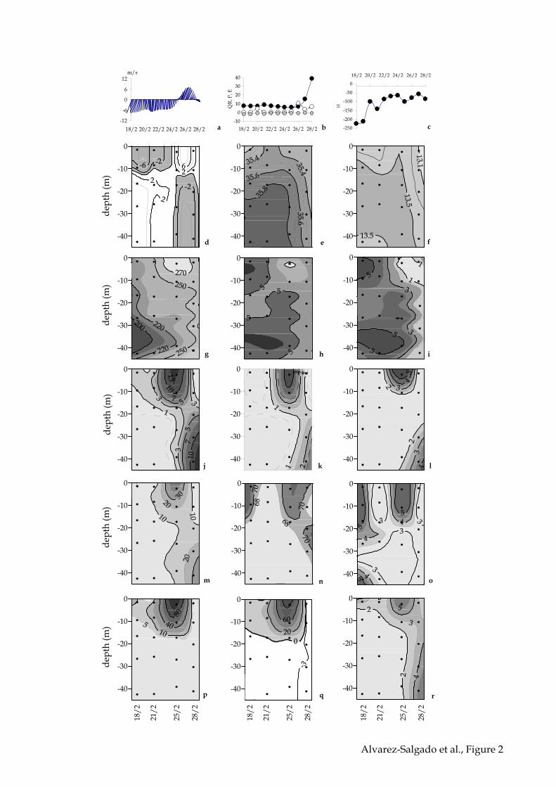
Figure 2. Time evolution of shelf winds, in m s–1 (a), continental runoff, precipitation
and evaporation, in m3 s–1 (b), heat balance, in cal cm–2 d–1 (c), residual currents, in cm
s–1 (d), salinity (e), temperature, in ºC (f), dissolved oxygen, in µmol kg–1 (g), total
inorganic nitrogen, in µmol k g–1 (h); silicate, in µmol k g–1 (i), Chlorophyll, in µg L–1
(j), fucoxanthin, in µg L–1 (k), suspended carbohydrates, in µmol L–1 (l), suspended
organic carbon, in µmol L–1 (m), dissolved organic carbon , in µmol L–1 (n), dissolved
carbohydrates, in µmol L–1 (o); gross primary production, in µmol kg–1 d–1 of O2 (p);
net primary production, µmol kg–1 d–1 of O2 (q); and respiration, µmol kg–1 d–1 of O2
(r). Panel b: black circles, continental runoff; grey circles, evaporation; open circles,
precipitation.
Figure 3. Ternary mixing diagram indicating the proportions of N and P compounds
(chlorophyll + proteins + P compounds), carbohydrates and lipids in the particulate
organic material of samples collected at stn 00. Solid dots, samples from stn 00; white
dots, riverine samples.
Figure 4. Results of the grazing incubation experiments conducted on 21 (open circles)
and 28 (solid circles) February 2002 with water of 10 m depth at stn 00. The logarithm
of the ratio between the final and initial Chlorophyll concentration is represented
against the dilution factor to obtain the corresponding phytoplankton growth
(intercept) and microzooplankton grazing (slope) rates.

8.95º 8.90º 8.85º 8.80º 8.75º 8.70º 8.65º 8.60º
Longitude (W)
42.15º
42.20º
42.25º
42.30º
42.35º
Latit
ude
(N)
Ría de Vigostn 00
Alvarez-Salgado et al., Figure 1
Figure 1
Silleiro buoy
Cies Islands
riverOitabén-2
50
-150
-100
-50-20
-50-75
-100
-12
-6
0
6
12
18/2 20/2 22/2 24/2 26/2 28/2
m/s
-100
10
2030
40
18/2 20/2 22/2 24/2 26/2 28/2
QR
, P, E
-250
-200
-150
-100
-50
0
18/2 20/2 22/2 24/2 26/2 28/2
H
-40
-30
-20
-10
0
-40
-30
-20
-10
0
-40
-30
-20
-10
0
a b c
d e f
g h i
j k l
m n o
p q
-40
-30
-20
-10
0
-40
-30
-20
-10
0
-40
-30
-20
-10
0
-40
-30
-20
-10
0
-40
-30
-20
-10
0
-40
-30
-20
-10
0
-40
-30
-20
-10
0
-40
-30
-20
-10
0
r-40
-30
-20
-10
0
-40
-30
-20
-10
0
-40
-30
-20
-10
0
Alvarez-Salgado et al., Figure 2
-40
-30
-20
-10
0
dept
h (m
)de
pth
(m)
dept
h (m
)de
pth
(m)
dept
h (m
)
18/2
21/2
25/2
28/2
18/2
21/2
25/2
28/2
18/2
21/2
25/2
28/2

Alvarez-Salgado et al., Figure 3
%lipids0 10 20 30 40 50 60
%N
/P
40
50
60
70
8020
30
40
50
60
70
0 20 40 60 80 1000
20
40
60
80
100
%CH
O
0
20
40
60
80
100

dilution
0.0 0.2 0.4 0.6 0.8 1.0
ln(C
t/C
0)
0.00
0.25
0.50
0.75
1.00
1.25
1.50
dilution
0.0 0.2 0.4 0.6 0.8 1.0
Alvarez-Salgado et al., Figure 4