orthogonal polynomials (in matlab)orthogonal polynomials (in matlab) walter gautschi...
TRANSCRIPT


Orthogonal Polynomials
• Recurrence coefficients• Modified Chebyshev algorithm• Discrete Stieltjes and Lanczos algorithm• Discretization methods• Modification algorithms
Sobolev Orthogonal Polynomials• Moment-based algorithm
• Discretization algorithm
• Zeros
OP.matlab – p. 2/29

Orthogonal Polynomials• Recurrence coefficients
• Modified Chebyshev algorithm• Discrete Stieltjes and Lanczos algorithm• Discretization methods• Modification algorithms
Sobolev Orthogonal Polynomials• Moment-based algorithm
• Discretization algorithm
• Zeros
OP.matlab – p. 2/29

Orthogonal Polynomials• Recurrence coefficients• Modified Chebyshev algorithm
• Discrete Stieltjes and Lanczos algorithm• Discretization methods• Modification algorithms
Sobolev Orthogonal Polynomials• Moment-based algorithm
• Discretization algorithm
• Zeros
OP.matlab – p. 2/29

Orthogonal Polynomials• Recurrence coefficients• Modified Chebyshev algorithm• Discrete Stieltjes and Lanczos algorithm
• Discretization methods• Modification algorithms
Sobolev Orthogonal Polynomials• Moment-based algorithm
• Discretization algorithm
• Zeros
OP.matlab – p. 2/29

Orthogonal Polynomials• Recurrence coefficients• Modified Chebyshev algorithm• Discrete Stieltjes and Lanczos algorithm• Discretization methods
• Modification algorithms
Sobolev Orthogonal Polynomials• Moment-based algorithm
• Discretization algorithm
• Zeros
OP.matlab – p. 2/29

Orthogonal Polynomials• Recurrence coefficients• Modified Chebyshev algorithm• Discrete Stieltjes and Lanczos algorithm• Discretization methods• Modification algorithms
Sobolev Orthogonal Polynomials• Moment-based algorithm
• Discretization algorithm
• Zeros
OP.matlab – p. 2/29

Orthogonal Polynomials• Recurrence coefficients• Modified Chebyshev algorithm• Discrete Stieltjes and Lanczos algorithm• Discretization methods• Modification algorithms
Sobolev Orthogonal Polynomials
• Moment-based algorithm
• Discretization algorithm
• Zeros
OP.matlab – p. 2/29
Orthogonal Polynomials• Recurrence coefficients• Modified Chebyshev algorithm• Discrete Stieltjes and Lanczos algorithm• Discretization methods• Modification algorithms
Sobolev Orthogonal Polynomials• Moment-based algorithm
• Discretization algorithm
• Zeros
OP.matlab – p. 2/29

Orthogonal Polynomials• Recurrence coefficients• Modified Chebyshev algorithm• Discrete Stieltjes and Lanczos algorithm• Discretization methods• Modification algorithms
Sobolev Orthogonal Polynomials• Moment-based algorithm
• Discretization algorithm
• Zeros
OP.matlab – p. 2/29

Orthogonal Polynomials• Recurrence coefficients• Modified Chebyshev algorithm• Discrete Stieltjes and Lanczos algorithm• Discretization methods• Modification algorithms
Sobolev Orthogonal Polynomials• Moment-based algorithm
• Discretization algorithm
• Zeros
OP.matlab – p. 2/29

Reference W. Gautschi, "Orthogonal Polynomials:Computation and Approximation", ClarendonPress, Oxford, 2004
http://www.cs.purdue.edu/homes/wxg/papers.html
click on Madrid.psalso in: Lecture Notes in Mathematics, 2007(?)
http://www.cs.purdue.edu/archives/2002/wxg/codes
OP.matlab – p. 3/29

Background
inner product
(p, q)dλ =
∫
R
p(t)q(t)dλ(t), dλ ≥ 0
orthogonal polynomials
πk( · ) = πk( · ; dλ) : (πk, π`)dλ
= 0, k 6= `
> 0, k = `
three-term recurrence relation
πk+1(t) = (t − αk)πk(t) − βkπk−1(t), k = 0, 1, . . . , n − 1
αk = αk(dλ) ∈ R, βk = βk(dλ) > 0(
β0 =∫
Rdλ(t)
)
OP.matlab – p. 4/29

Jacobi Matrix
of infinite order
J(dλ) =
α0
√β1 0√
β1 α1
√β2√
β2 α2. . .
. . . . . .0
of order n
Jn(dλ) = J(dλ)[1:n,1:n]
OP.matlab – p. 5/29

"Classical" Weight Functions
dλ(t) = w(t)dt
name w(t) on
Jacobi (1 − t)α(1 + t)β [−1, 1]
Laguerre tαe−t [0,∞]
Hermite |t|2αe−t2 [−∞,∞]
OP.matlab – p. 6/29

Matlab
example: ab=r jacobi(N,a,b)
α0 β0
α1 β1... ...
αN−1 βN−1
N ∈ N, a > −1, b > −1
ab
OP.matlab – p. 7/29

Demo #1N=10;ab=r jacobi(N,-.5,1.5);
k αk βk0 0.66666666666667 4.712388980384691 0.13333333333333 0.138888888888892 0.05714285714286 0.210000000000003 0.03174603174603 0.229591836734694 0.02020202020202 0.237654320987655 0.01398601398601 0.241735537190086 0.01025641025641 0.244082840236697 0.00784313725490 0.245555555555568 0.00619195046440 0.246539792387549 0.00501253132832 0.24722991689751
OP.matlab – p. 8/29

Modified Chebyshev Algorithm
modified moments
mk =
∫
R
pk(t)dλ(t), k = 0, 1, 2, . . .
modified moment map
R2n 7→ R
2n : [mk]2n−1k=0 7→ [αk, βk]
n−1k=0
algorithm: Sack et al., 1971; Wheeler, 1974conditioning: G.,1968; 1982
Matlabab=chebyshev(N,mom,abm)
OP.matlab – p. 9/29

Modified Chebyshev Algorithmmodified moments
mk =
∫
R
pk(t)dλ(t), k = 0, 1, 2, . . .
modified moment map
R2n 7→ R
2n : [mk]2n−1k=0 7→ [αk, βk]
n−1k=0
algorithm: Sack et al., 1971; Wheeler, 1974conditioning: G.,1968; 1982
Matlabab=chebyshev(N,mom,abm)
OP.matlab – p. 9/29

Modified Chebyshev Algorithmmodified moments
mk =
∫
R
pk(t)dλ(t), k = 0, 1, 2, . . .
modified moment map
R2n 7→ R
2n : [mk]2n−1k=0 7→ [αk, βk]
n−1k=0
algorithm: Sack et al., 1971; Wheeler, 1974conditioning: G.,1968; 1982
Matlabab=chebyshev(N,mom,abm)
OP.matlab – p. 9/29

Modified Chebyshev Algorithmmodified moments
mk =
∫
R
pk(t)dλ(t), k = 0, 1, 2, . . .
modified moment map
R2n 7→ R
2n : [mk]2n−1k=0 7→ [αk, βk]
n−1k=0
algorithm: Sack et al., 1971; Wheeler, 1974conditioning: G.,1968; 1982
Matlabab=chebyshev(N,mom,abm)
OP.matlab – p. 9/29

Demo #2elliptic orthogonal polynomials
dλ(t) = [(1 − ω2t2)(1 − t2)]−1/2dt on [−1, 1],
0 ≤ ω < 1
Chebyshev moments
m0 =∫ 1
−1 dλ(t), mk = 12k−1
∫ 1
−1 Tk(t)dλ(t), k ≥ 1
Matlab
function ab=r elliptic(N,om2)abm=r jacobi(2*N-1,-1/2);mom=mm elliptic(N,om2);ab=chebyshev(N,mom,abm);
OP.matlab – p. 10/29

Demo #2elliptic orthogonal polynomials
dλ(t) = [(1 − ω2t2)(1 − t2)]−1/2dt on [−1, 1],
0 ≤ ω < 1Chebyshev moments
m0 =∫ 1
−1 dλ(t), mk = 12k−1
∫ 1
−1 Tk(t)dλ(t), k ≥ 1
Matlab
function ab=r elliptic(N,om2)abm=r jacobi(2*N-1,-1/2);mom=mm elliptic(N,om2);ab=chebyshev(N,mom,abm);
OP.matlab – p. 10/29

Demo #2elliptic orthogonal polynomials
dλ(t) = [(1 − ω2t2)(1 − t2)]−1/2dt on [−1, 1],
0 ≤ ω < 1Chebyshev moments
m0 =∫ 1
−1 dλ(t), mk = 12k−1
∫ 1
−1 Tk(t)dλ(t), k ≥ 1
Matlab
function ab=r elliptic(N,om2)abm=r jacobi(2*N-1,-1/2);mom=mm elliptic(N,om2);ab=chebyshev(N,mom,abm);
OP.matlab – p. 10/29

Demo #2 (cont’)
ω2 = .999, N = 40
k βk k βk k βk k βk
0 9.68226512 10 0.24936494 20 0.24992062 30 0.249980621 0.79378214 11 0.24951641 21 0.24993230 31 0.249982882 0.11986767 12 0.24962381 22 0.24994197 32 0.249984853 0.22704012 13 0.24970218 23 0.24995003 33 0.249986574 0.24106088 14 0.24976074 24 0.24995679 34 0.249988065 0.24542853 15 0.24980537 25 0.24996249 35 0.249989376 0.24730165 16 0.24983998 26 0.24996732 36 0.249990527 0.24825871 17 0.24986721 27 0.24997145 37 0.249991548 0.24880566 18 0.24988890 28 0.24997497 38 0.249992439 0.24914365 19 0.24990639 29 0.24997800 39 0.24999322
OP.matlab – p. 11/29

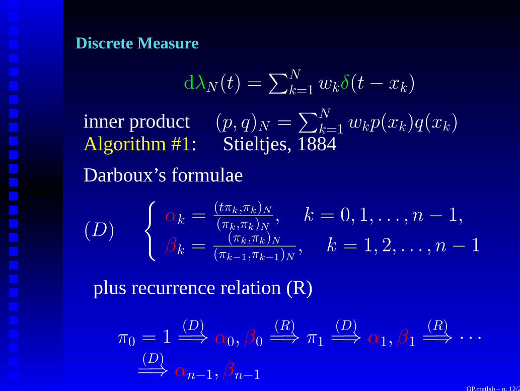
Discrete Measure
dλN(t) =∑N
k=1 wkδ(t − xk)
inner product (p, q)N =∑N
k=1 wkp(xk)q(xk)Algorithm #1: Stieltjes, 1884
Darboux’s formulae
(D)
{
αk = (tπk,πk)N
(πk,πk)N
, k = 0, 1, . . . , n − 1,
βk = (πk,πk)N
(πk−1,πk−1)N
, k = 1, 2, . . . , n − 1
plus recurrence relation (R)
π0 = 1(D)=⇒ α0, β0
(R)=⇒ π1
(D)=⇒ α1, β1
(R)=⇒ · · ·
(D)=⇒ αn−1, βn−1
OP.matlab – p. 12/29

Algorithm #2 Lanczos, 1950
QT
1√
w1
√w2 ··· √
wN√w1 x1 0 ··· 0√w2 0 x2 ··· 0... ... ... . . . ...√wN 0 0 ··· xN
Q
=
1√
β0 0 ··· 0√β0 α0
√β1 ··· 0
0√
β1 α1 ··· 0... ... ... . . . ...0 0 0 ··· αN−1
stable version of Lanczos algorithmRutishauser, 1963; Gragg and Harrod, 1984
OP.matlab – p. 13/29

Matlab
ab=stieltjes(n,xw)ab=lanczos(n,xw)
}
n ≤ N
x1 w1
x2 w2... ...
xN wN
xw
OP.matlab – p. 14/29

Discretization Methods G.; 1968, 1982
basic idea
dλ(t) ≈ dλN(t),
{
αk(dλ) ≈ αk(dλN)
βk(dλ) ≈ βk(dλN)example
w(t) = (1 − t2)−1/2 + c on [−1, 1], c > 0
discretization
(p, q) =∫ 1
−1 p(t)q(t)(1 − t2)−1/2dt + c∫ 1
−1 p(t)q(t)dt
≈∑N
k=1 wChk p(xCh
k )q(xChk ) + c
∑Nk=1 wL
k p(xLk )q(xL
k )
OP.matlab – p. 15/29

Discretization Methods G.; 1968, 1982
basic idea
dλ(t) ≈ dλN(t),
{
αk(dλ) ≈ αk(dλN)
βk(dλ) ≈ βk(dλN)
example
w(t) = (1 − t2)−1/2 + c on [−1, 1], c > 0
discretization
(p, q) =∫ 1
−1 p(t)q(t)(1 − t2)−1/2dt + c∫ 1
−1 p(t)q(t)dt
≈∑N
k=1 wChk p(xCh
k )q(xChk ) + c
∑Nk=1 wL
k p(xLk )q(xL
k )
OP.matlab – p. 15/29

Discretization Methods G.; 1968, 1982
basic idea
dλ(t) ≈ dλN(t),
{
αk(dλ) ≈ αk(dλN)
βk(dλ) ≈ βk(dλN)example
w(t) = (1 − t2)−1/2 + c on [−1, 1], c > 0
discretization
(p, q) =∫ 1
−1 p(t)q(t)(1 − t2)−1/2dt + c∫ 1
−1 p(t)q(t)dt
≈∑N
k=1 wChk p(xCh
k )q(xChk ) + c
∑Nk=1 wL
k p(xLk )q(xL
k )
OP.matlab – p. 15/29

Discretization Methods G.; 1968, 1982
basic idea
dλ(t) ≈ dλN(t),
{
αk(dλ) ≈ αk(dλN)
βk(dλ) ≈ βk(dλN)example
w(t) = (1 − t2)−1/2 + c on [−1, 1], c > 0
discretization
(p, q) =∫ 1
−1 p(t)q(t)(1 − t2)−1/2dt + c∫ 1
−1 p(t)q(t)dt
≈∑N
k=1 wChk p(xCh
k )q(xChk ) + c
∑Nk=1 wL
k p(xLk )q(xL
k )
OP.matlab – p. 15/29

in general
discretize dλ ons
⋃
j=1
[aj, bj]
using
tailor-made quadratures
general-purpose quadratures
on each [aj, bj]
OP.matlab – p. 16/29

Matlab
ab=mcdis(n,eps0,quad,Nmax)
structure (global variables)
mc, mp, iq
AB =
a1 b1
a2 b2... ...
amc bmc
, DM =
x1 y1
x2 y2... ...
xmp ymp
OP.matlab – p. 17/29

example w(t) = tαK0(t) on [0,∞], α > −1
K0(t) =
{
R(t) + I0(t) ln(1/t) if 0 < t ≤ 1,
t−1/2e−tS(t) if 1 ≤ t < ∞,∫ ∞
0 f(t)w(t)dt
=∫ 1
0 [R(t)f(t)]tαdt +∫ 1
0 [I0(t)f(t)]tα ln(1/t)dt
+ e−1∫ ∞
0 [(1 + t)α−1/2S(1 + t)f(1 + t)]e−tdt
AB=0 10 10 ∞
w1(t) = tα
w2(t) = tα ln(1/t)
w3(t) = e−t
OP.matlab – p. 18/29

example w(t) = tαK0(t) on [0,∞], α > −1
K0(t) =
{
R(t) + I0(t) ln(1/t) if 0 < t ≤ 1,
t−1/2e−tS(t) if 1 ≤ t < ∞,
∫ ∞0 f(t)w(t)dt
=∫ 1
0 [R(t)f(t)]tαdt +∫ 1
0 [I0(t)f(t)]tα ln(1/t)dt
+ e−1∫ ∞
0 [(1 + t)α−1/2S(1 + t)f(1 + t)]e−tdt
AB=0 10 10 ∞
w1(t) = tα
w2(t) = tα ln(1/t)
w3(t) = e−t
OP.matlab – p. 18/29

example w(t) = tαK0(t) on [0,∞], α > −1
K0(t) =
{
R(t) + I0(t) ln(1/t) if 0 < t ≤ 1,
t−1/2e−tS(t) if 1 ≤ t < ∞,∫ ∞
0 f(t)w(t)dt
=∫ 1
0 [R(t)f(t)]tαdt +∫ 1
0 [I0(t)f(t)]tα ln(1/t)dt
+ e−1∫ ∞
0 [(1 + t)α−1/2S(1 + t)f(1 + t)]e−tdt
AB=
0 1
0 1
0 ∞
w1(t) = tα
w2(t) = tα ln(1/t)
w3(t) = e−t
OP.matlab – p. 18/29

Modification Algorithms G., 1982
problem: given the recurrence coefficients of dλ,generate those of
dλmod(t) = r(t)dλ(t), r ≥ 0 on supp(dλ), rational
example: Galant, 1971
r(t) = s(t − c), c ∈ R\supp(dλ), s = ±1
one step of (symmetric) LR algorithm:
s[Jn+1(dλ) − cI] = LLT
Jn(dλmod) =(
LTL + cI)
[1:n,1:n]
nonlinear recurrence algorithm
OP.matlab – p. 19/29

Matlab
ab=chri1(N,ab0,c), chri2, . . ., chri8
application: induced orthogonal polynomials(G. and Li, 1993)
dλmod(t) = [πm(t; dλ)]2dλ(t)
[πm(t; dλ)]2 =m
∏
µ=1
(t − τµ)2
m consecutive modifications by quadratic factors
OP.matlab – p. 20/29

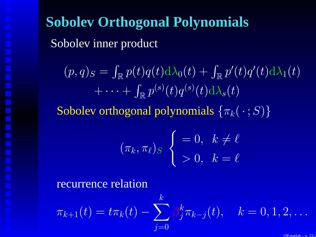
Sobolev Orthogonal Polynomials
Sobolev inner product
(p, q)S =∫
Rp(t)q(t)dλ0(t) +
∫
Rp′(t)q′(t)dλ1(t)
+ · · · +∫
Rp(s)(t)q(s)(t)dλs(t)
Sobolev orthogonal polynomials {πk( · ; S)}
(πk, π`)S
{
= 0, k 6= `
> 0, k = `
recurrence relation
πk+1(t) = tπk(t) −k
∑
j=0
βkjπk−j(t), k = 0, 1, 2, . . .
OP.matlab – p. 21/29

Sobolev Orthogonal PolynomialsSobolev inner product
(p, q)S =∫
Rp(t)q(t)dλ0(t) +
∫
Rp′(t)q′(t)dλ1(t)
+ · · · +∫
Rp(s)(t)q(s)(t)dλs(t)
Sobolev orthogonal polynomials {πk( · ; S)}
(πk, π`)S
{
= 0, k 6= `
> 0, k = `
recurrence relation
πk+1(t) = tπk(t) −k
∑
j=0
βkjπk−j(t), k = 0, 1, 2, . . .
OP.matlab – p. 21/29

Recurrence Matrixrecurrence relation
πk+1(t) = tπk(t) −k
∑
j=0
βkjπk−j(t), k = 0, 1, 2, . . .
matrix of recurrence coefficients
Bn =
β00 β1
1 β22 · · · βn−2
n−2 βn−1n−1
1 β10 β2
1 · · · βn−2n−3 βn−1
n−2
0 1 β20 · · · βn−2
n−4 βn−1n−3
· · · · · · · · · · · · · · · · · ·0 0 0 · · · βn−2
0 βn−11
0 0 0 · · · 1 βn−10
OP.matlab – p. 22/29

Modified Chebyshev Algorithm
modified moments
m(σ)k =
∫
Rpk(t)dλσ,
k = 0, 1, 2, . . . , ; σ = 0, 1, . . . , s
modified moment map
[m(σ)k ]2n−1
k=0 , σ = 0, 1, . . . , s 7→ Bn
algorithm G. and Zhang, 1995conditioning Zhang, 1994
Matlab (for s = 1)B=chebyshev sob(N,mom,abm)
OP.matlab – p. 23/29

Modified Chebyshev Algorithmmodified moments
m(σ)k =
∫
Rpk(t)dλσ,
k = 0, 1, 2, . . . , ; σ = 0, 1, . . . , s
modified moment map
[m(σ)k ]2n−1
k=0 , σ = 0, 1, . . . , s 7→ Bn
algorithm G. and Zhang, 1995
conditioning Zhang, 1994
Matlab (for s = 1)B=chebyshev sob(N,mom,abm)
OP.matlab – p. 23/29

Modified Chebyshev Algorithmmodified moments
m(σ)k =
∫
Rpk(t)dλσ,
k = 0, 1, 2, . . . , ; σ = 0, 1, . . . , s
modified moment map
[m(σ)k ]2n−1
k=0 , σ = 0, 1, . . . , s 7→ Bn
algorithm G. and Zhang, 1995
conditioning Zhang, 1994
Matlab (for s = 1)B=chebyshev sob(N,mom,abm)
OP.matlab – p. 23/29

Modified Chebyshev Algorithmmodified moments
m(σ)k =
∫
Rpk(t)dλσ,
k = 0, 1, 2, . . . , ; σ = 0, 1, . . . , s
modified moment map
[m(σ)k ]2n−1
k=0 , σ = 0, 1, . . . , s 7→ Bn
algorithm G. and Zhang, 1995
conditioning Zhang, 1994
Matlab (for s = 1)B=chebyshev sob(N,mom,abm)
OP.matlab – p. 23/29

example dλ0(t) = dt, dλ1(t) = γdt on [−1, 1](Althammer, 1962)
modified moments
pk(t) = monic Legendre
m(0)0 = 2, m
(1)0 = 2γ; m
(0)k = m
(1)k = 0, k > 0
Matlab
mom=zeros(2,2*N);mom(1,1)=2; mom(2,1)=2*g;abm=r jacobi(2*N-1);B=chebyshev sob(N,mom,abm);
OP.matlab – p. 24/29

Discretized Stieltjes Algorithm
(G. and Zhang, 1995)
βkj =
(tπk, πk−j)S
(πk−j, πk−j)S, j = 0, 1, . . . , k
Gauss quadrature discretization
(p, q)dλσ≈
nσ∑
k=1
w(σ)k p(x
(σ)k )q(x
(σ)k ), σ = 0, 1, . . . , s
MatlabB=stieltjes sob(N,s,nd,xw,a0,same)md=max(nd), a0=α0(dλ0)
OP.matlab – p. 25/29

Discretized Stieltjes Algorithm(G. and Zhang, 1995)
βkj =
(tπk, πk−j)S
(πk−j, πk−j)S, j = 0, 1, . . . , k
Gauss quadrature discretization
(p, q)dλσ≈
nσ∑
k=1
w(σ)k p(x
(σ)k )q(x
(σ)k ), σ = 0, 1, . . . , s
MatlabB=stieltjes sob(N,s,nd,xw,a0,same)md=max(nd), a0=α0(dλ0)
OP.matlab – p. 25/29

Discretized Stieltjes Algorithm(G. and Zhang, 1995)
βkj =
(tπk, πk−j)S
(πk−j, πk−j)S, j = 0, 1, . . . , k
Gauss quadrature discretization
(p, q)dλσ≈
nσ∑
k=1
w(σ)k p(x
(σ)k )q(x
(σ)k ), σ = 0, 1, . . . , s
MatlabB=stieltjes sob(N,s,nd,xw,a0,same)md=max(nd), a0=α0(dλ0)
OP.matlab – p. 25/29

Matlab (cont’)
xw=
x(0)1 · · · x
(s)1 w
(0)1 · · · w
(s)1
x(0)2 · · · x
(s)2 w
(0)2 · · · w
(s)2
... ... ... ...
x(0)md · · · x
(s)md w
(0)md · · · w
(s)md
OP.matlab – p. 26/29

example Althammer’s polynomials
Matlabs=1; nd=[N N];a0=0; same=1;ab=r jacobi(N);zw=gauss(N,ab);xw=[zw(:,1) zw(:,1) ...
zw(:,2) g*zw(:,2)];B=stieltjes sob(N,s,nd,xw,a0,same);
OP.matlab – p. 27/29
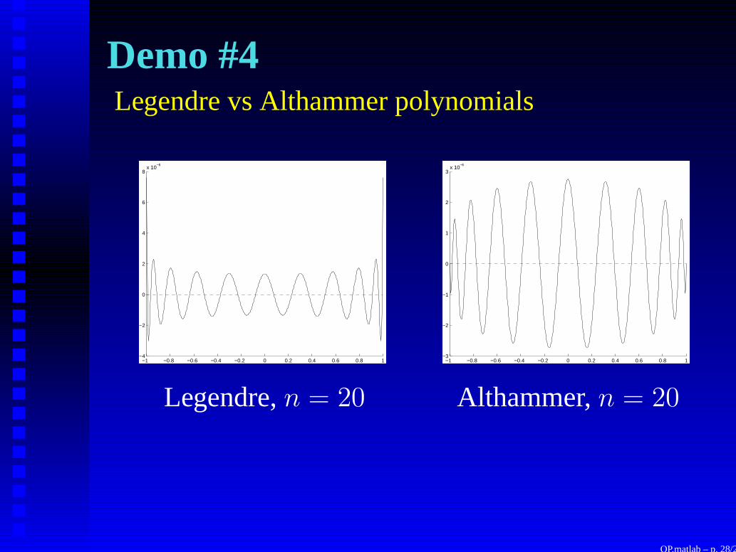
Demo #4Legendre vs Althammer polynomials
−1 −0.8 −0.6 −0.4 −0.2 0 0.2 0.4 0.6 0.8 1−4
−2
0
2
4
6
8x 10
−6
−1 −0.8 −0.6 −0.4 −0.2 0 0.2 0.4 0.6 0.8 1−3
−2
−1
0
1
2
3x 10
−6
Legendre, n = 20 Althammer, n = 20
OP.matlab – p. 28/29

Zeros
ifπT (t) = [π0(t), π1(t), . . . , πn−1(t)]
thentπT (t) = πT (t)Bn + πn(t)e
Tn
Theorem The zeros τν of πn are the eigenvalues of Bn
and πT (τν) corresponding (left) eigenvectors.
Matlabz=sobzeros(n,N,B)
OP.matlab – p. 29/29