osaka university graduate school of medicine vfm atlas

■日立アロカメディカル　製品カタログ 16P　H1-4　D案　2013.11.08

Vector Flow Mapping AtlasV FM ATL AS

6-22-1, Mure, Mitaka-shi, Tokyo, 181-8622, Japan　

Telephone : +81 422 45 5122　Facsimile : +81 422 45 4058　Website : http://www.hitachi-aloka.co.jp/english/Printed in Japan MC2014(149)TH

Satoshi Nakatani:Department of Functional Diagnostic Science, Area of Medical Technology and Science, Osaka University Graduate School of Medicine

Marie Stugaard:Department of Functional Diagnostic Science, Area of Medical Technology and Science, Osaka University Graduate School of Medicine

Tokuhisa Uejima:Department Of Cardiology, Cardiovascular Institute Hospital

Yoshihiro Seo:Cardiovascular Division, University of Tsukuba

Tomoko Ishizu:Cardiovascular Division, University of Tsukuba

Nobuyuki Ohte:Department of Cardio-Renal Medicine and Hypertension,Nagoya City University

Takashi Honda:Department of Pediatrics, Kitasato University Hospital

Taiyu Hayashi:Department of Pediatrics, University of Tokyo

Clinical Cases

Supervisor

Katsu Takenaka:Division of Cardiology, Department of Medicine, Nihon University School of Medicine;Department of Clinical Laboratory, University of Tokyo Hospital

Keiichi Itatani:Departments of Cardiovascular Surgery and Hemodynamic Analysis,Kitasato University School of Medicine

Tokuhisa Uejima:Department Of Cardiology, Cardiovascular Institute Hospital

■日立アロカメディカル　製品カタログ 16P　H1-4　B案　2013.11.18.

1 2

Vector Flow Mapping (VFM)

Vector flow mapping is a technique to visualize blood flow and flow velocity in the heart.

<Healthy heart>

Color DopplerDiastolic phase Systolic phase

Principle of Vector Flow Mapping (VFM)Keiichi ItataniPrinciples of the method for vector calculation by preservation of flow rate in the cross-section �� 2

Ultrasound imaging method for VFM based on the VFM basic theory �� 4

Calculation method of hemodynamics index �� 5

Vorticity and circulation �� 5

Energy loss of blood flow �� 6

Wall Shear Stress �� 6

Verification ExperimentVerification of flow velocity vectors obtained by VFMTakashi Okada �� 7

Case ExamplesVFM in Normal Subjects Marie Stugaard and Satoshi Nakatani �� 9

Status after valve replacement Tokuhisa Uejima �� 10

A case with a left ventricular apical aneurysm Nobuyuki Ohte �� 11

Flow pattern in left ventricular dysfunction with and without dyssynchrony Tomoko Ishizu and Yoshihiro Seo �� 12

A newborn with double outlet right ventricle, transposition of the great arteries, coarctation of the aorta, and patent ductus arteriosus Takashi Honda �� 13

Single ventricleTaiyu Hayashi �� 14

Contents

To represent flow rate as a vector in a two-dimensional measured cross-section, flow velocity components of two orthogonal directions are required. Since the flow velocity to the direction of the beam emitted from the probe can be obtained by color Doppler on electrocardiography, the component orthogonal to it (the flow velocity to the direction orthogonal to the beam) is required (Figure 2). However, it is estimated by calculation since a distribution of flow velocity to the direction orthogonal to the beam cannot be obtained by actual measurement.

Direction

orthogonal to

the beam θ

Beam

direction r

Figure 2: Direction of the Beam Emitted from the Probe and Direction Orthogonal to the Beam

preservation of flow rate in the cross-sectionPrinciples of the method for vector calculation by

Principle of Vector Flow Mapping (VFM)

VFM is a method to present blood flow as a vector distribution, which enables easy acquisition of vector distributions of cardiac and vascular lumens only based on 2D cross-sectional images obtained by B-mode color Doppler. The data required for VFM analysis is only a B-mode black-and-white moving image of the ventricle and blood vessels combined with a color Doppler data of the lumen. A B-mode black-and-white moving image is required to perform speckle tracking of the cardiac and vascular walls.

Keiichi Itatani: Departments of Cardiovascular Surgery and Hemodynamic Analysis, Kitasato University School of Medicine

Figure 1: Structure of Vector Flow Mapping (VFM)

Color Doppler Speckle tracking Vector Flow Mapping (VFM)

The principles of preservation of flow rate in the cross-section (continuity equation) is used to calculate the flow velocity to the direction orthogonal to the beam. The continuity equation is an equation to preserve the flow rate at the point where the blood flow comes in and out, which is often used for calculation of the valve area in aortic valve stenosis (Figure 3).The basic relation is:

Inflow rate = Outflow rate

In addition, the relation of the flow rate and the flow velocity is:

Flow rate = Flow velocity x Area of the cross-section to pass through , and

Flow rate = Flow velocity x Length of the line to pass through for 2D image.

■日立アロカメディカル　製品カタログ 16P　P2-P3　2013.11.18.

3 4

Thus, since preservation of the flow rate for 2D measured cross-sections is assumed VFM, measurement should be performed by selecting a cross-section where the main flownes in and the flow rate can pass through is small enough to ignore compared to the flow in cross-section.

Concentric circles are depicted in the direction of a certain depth using beams emitted from the probe and sampling points of each beam on the cross-section measured by echocardiography, and the measured cross-section is virtually divided using a tiny square mesh (Figure 2). Then, the flow rate should be preserved based on the continuity equation in each mesh element (square cell) (Figure 3). Based on this, the flow velocity to the direction orthogonal to the beam (transverse) is calculated from the transverse flow rate. First, the transverse flow velocity can be obtained from the wall motion velocity measured by speckle tracking in the square cells near the cardiac/vascular wall. Then, as shown in (2) of Figure 4, the inflow and outflow rates of the square cells can be obtained for three directions based on the flow velocity components for these three directions. Therefore, the transverse flow velocity for the remaining one direction can be obtained by subtracting the data for the three directions.

Since the transverse flow velocity for one of the two directions is similarly obtained in the cells next to the cells near the wall ((3) of Figure 4), the transverse flow velocity for the remaining one direction is calculated from the transverse flow rate so that the inflow rate and outflow rate are equal, along with the longitudinal flow velocity for two directions obtained by color Doppler. Thus, if the transverse flow velocity can be obtained at all measurement points in the cardiac lumen, combined with the information obtained by color Doppler, longitudinal and transverse flow velocity components can be obtained. Then, the flow velocity can be obtained as a vector at each point in the measured plane, and blood flow can be represented as a distribution of vectors.

Lumen Micro square

Inflow rate = Outflow rateA1 u1 = A2 u2

Inflow rate = Outflow rate :

Transversal flow rate + longitudinal flow rate

A1A2

u1

u2

u1 = Flow velocity going into the lumen

A1 = Cross sectional area of lumen where the flow passes through at the flow rate of u1

u2 = Flow velocity coming out of lumen

A2 = Cross sectional area of lumen where the flow passes through at the flow rate of u2

u, v = Flow velocity coming out of the square

l1, l2 = Length of line where the flow passes through at the flow rate of u,v

Figure 3: Continuity Equation and Preservation of Flow Rate

Figure 4: Method to calculate transverse flow velocity

1) Longitudinal flow velocity by color Doppler and wall velocity by speckle tracking

2) Preservation of flow rate in the cells near the wall ⇒ Calculation of transverse flow velocity

3) Transverse flow velocity is calculated sequentially from the cells near the wall

4) Distribution of transverse flow velocities is calculated

5) Vectors are calculated based on longitudinal and transverse flow velocities

6) VFM vectors are calculated

Figure 4-(1) Figure 4-(2) Figure 4-(3)

Figure 4-(4) Figure 4-(5) Figure 4-(6)

Longitudinal flow velocity by color Doppler

wall velocity by speckle tracking

Transverse flow velocity Vectors

Based on the above theory, the tips and considerations for imaging required for analysis using VFM are as follows:

1) The color Doppler window covers the entire cardiac lumen.2) The wall of the cardiac lumen or vascular wall on both sides were clearly obtained as B-mode image.3) The Nyquist frequency is set so that aliasing on color Doppler is as small as possible.4) The frame rate is set to be as high as possible.

the VFM basic theoryUltrasound imaging method for VFM based on

In VFM, which enables visualization of the distribution of flow velocity vectors, various parameters formalized rheologically can be calculated and hemodynamic parameters2) which can be only presented diagrammatically in a textbook of physiology or calculated using computational fluid dynamics (CFD, fluidic simulation using a computer) so far, such as Wall Shear Stress, energy loss of blood flow, etc. can be presented as actual values based on measurements. VFM is limited to two-dimensional flows, but at present, is a modality that enables measurement of hemodynamic parameters based on actual values.

Calculation method of hemodynamics index


5 6

References1) Itatani K, Okada T, Uejima T, Tanaka T, Ono M, Miyaji K, Takenaka K. Intraventricular flow velocity vector visualization based on the continuity

equation and measurements of vorticity and Wall Shear Stress. Jpn J Appl Pysic in-press2) Sengupta PP, Pedrizzetti G, Kilner PJ, Kheradvar A, Ebbers T, Tonti G, Fraser A, Narula J. Emergin trends in CV flow visualization: J Am Coll

Cardiol Img 5 (2012) 305-16

Stenosis of the vascularanastomosis site

⇒Jet blood flow⇒Rapid acceleration⇒Heterogeneous vectors

Shape of the vascularanastomosis site

⇒Turbulent flows⇒Heterogeneous vectors

Stenosis of the heart valve

⇒Jet blood flow⇒Rapid acceleration⇒Heterogeneous vectors

Valvular regurgitation

⇒Turbulent flows⇒Heterogeneous vectors

Figure 6: Pathological blood flow causing large energy loss

Blood is viscous and generates frictional heat due to viscosity at the site where turbulent flows occur. The energy of this frictional heat is called energy loss of blood flow.1) The intensity of turbulent flows is presented based on the extent of spatial dispersion of flow velocity vectors, by multiplying which energy loss is calculated. Energy loss is large at the site where a large change of vectors is locally seen and small at the laminar flow site, the site where a great-river-like, large systematic vortex is formed, or the almost flow-less site.Clinically, an image shown in Figure 6 below is easy to understand. For instance, jet blood flow occurs at the stenosis of the vascular anastomosis site or the stenosis of the heart valve, and even when the vascular anastomosis is not narrowed, if the bad shape causes turbulent flows mainly including vortexes, or if turbulent flows occur in the heart due to valvular regurgitation, disturbance of flow velocity vectors causes large energy loss. Of course, at the site where acceleration of the jet is too fast and reaches several times the nyquist limit, which causes many aliasing patterns on color Doppler, accurate calculation of vectors itself is difficult on VFM and the values of energy loss become inaccurate. These blood flows are the limit of VFM that calculates flow velocity vectors based on color Doppler.

Energy loss of blood flow

Figure 5: Vorticity mapping

Vorticity refers to the direction and intensity of the rotating movement of flow velocity vectors at a focal point. Flow velocity vectors have longitudinal components and transverse components, both of which increases/decreases to the longitudinal direction and transverse direction. For instance, to calculate the intensity of the counterclockwise (sinistral) rotating movement, the longitudinal increase/decrease of the transverse flow velocity should be subtracted from the transverse increase/decrease of the longitudinal flow velocity. This is defined as vorticity.

Vorticity = (Transverse increase/decrease of longitudinal flow velocity) – (Longitudinal increase/decrease of transverse flow velocity)

Vorticity with a positive value indicates the occurrence of an intensive, sinistral rotating flow at the place (indicated with a red scale), while vorticity with a negative value indicates the occurrence of an intensive, dextral rotating flow at the place (indicated with a blue scale) (Figure 5).

Vorticity and circulation

Circulation is an index showing the direction and intensity of the rotational force to the part surrounded with a closed curve and is presented as a value calculated by summing up all flow velocity components involved in a whole rotating movement on the curve.This is also theoretically consistent with the sum of vorticities in the surrounded area.

Wall Shear Stress is a force of blood flow to rub the endocardium/vascular intima, which can be calculated from the gradient of flow velocity near the wall. Wall Shear Stress is considered involved in intimal degeneration and breakdown of plaques and is a clinically useful index.

Wall Shear Stress


7 8

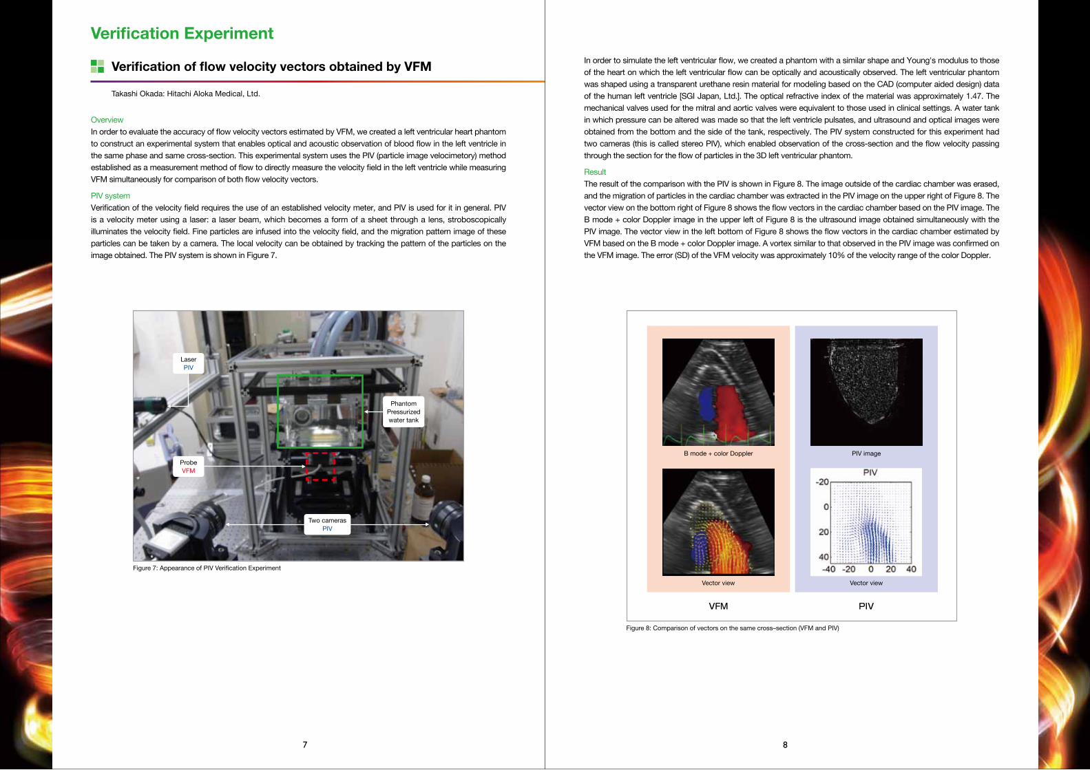
In order to simulate the left ventricular flow, we created a phantom with a similar shape and Young's modulus to those of the heart on which the left ventricular flow can be optically and acoustically observed. The left ventricular phantom was shaped using a transparent urethane resin material for modeling based on the CAD (computer aided design) data of the human left ventricle [SGI Japan, Ltd.]. The optical refractive index of the material was approximately 1.47. The mechanical valves used for the mitral and aortic valves were equivalent to those used in clinical settings. A water tank in which pressure can be altered was made so that the left ventricle pulsates, and ultrasound and optical images were obtained from the bottom and the side of the tank, respectively. The PIV system constructed for this experiment had two cameras (this is called stereo PIV), which enabled observation of the cross-section and the flow velocity passing through the section for the flow of particles in the 3D left ventricular phantom.

ResultThe result of the comparison with the PIV is shown in Figure 8. The image outside of the cardiac chamber was erased, and the migration of particles in the cardiac chamber was extracted in the PIV image on the upper right of Figure 8. The vector view on the bottom right of Figure 8 shows the flow vectors in the cardiac chamber based on the PIV image. The B mode + color Doppler image in the upper left of Figure 8 is the ultrasound image obtained simultaneously with the PIV image. The vector view in the left bottom of Figure 8 shows the flow vectors in the cardiac chamber estimated by VFM based on the B mode + color Doppler image. A vortex similar to that observed in the PIV image was confirmed on the VFM image. The error (SD) of the VFM velocity was approximately 10% of the velocity range of the color Doppler.

Figure 8: Comparison of vectors on the same cross–section (VFM and PIV)

VFM

B mode + color Doppler

Vector view

PIV image

Vector view

PIV

OverviewIn order to evaluate the accuracy of flow velocity vectors estimated by VFM, we created a left ventricular heart phantom to construct an experimental system that enables optical and acoustic observation of blood flow in the left ventricle in the same phase and same cross-section. This experimental system uses the PIV (particle image velocimetory) method established as a measurement method of flow to directly measure the velocity field in the left ventricle while measuring VFM simultaneously for comparison of both flow velocity vectors.

PIV systemVerification of the velocity field requires the use of an established velocity meter, and PIV is used for it in general. PIV is a velocity meter using a laser: a laser beam, which becomes a form of a sheet through a lens, stroboscopically illuminates the velocity field. Fine particles are infused into the velocity field, and the migration pattern image of these particles can be taken by a camera. The local velocity can be obtained by tracking the pattern of the particles on the image obtained. The PIV system is shown in Figure 7.

PhantomPressurizedwater tank

Figure 7: Appearance of PIV Verification Experiment

LaserPIV

ProbeVFM

Two camerasPIV

Takashi Okada: Hitachi Aloka Medical, Ltd.

Verification of flow velocity vectors obtained by VFM

Verification Experiment


9 10

Figure 17: Vector mapping (diastole). Inflow moves in the direction of the ventricular septum, and a large vortex rotating counterclockwise is formed.

Apical long axis view

Figure 19: Vector and Vorticity mapping (diastole)

Figure 18: Vector mapping (late diastole). The vortex slows down while decreasing in size, and another vortex is formed at the apex.

Figure 20: Energy loss mapping (diastole). Dissipation of large energy is seen in the vortex.

Flow patterns observed in the left ventricle with a prosthetic mitral valve are quite different from those in the normal left ventricle. This 78 year-old women underwent aortic and mitral valve replacement with mechanical valves 10 years ago. Flows across the mitral valve were directed toward the interventricular septum and formed a large vortex which rotated counter-clockwise (Figure 17). The vortex decreased in size and flows inside decelerated (figure 18). During the systole, the flow accelerated and ejected from the left ventricle. The direction of the vortex rotation can be identified in vector flow maps, but you can easily recognise the direction in vorticity maps. The counter-clockwise rotation of the large vortex during the diastole was depicted in red in the vorticity map (Figure 19). In the energy loss map, you can see that the energy dissipated in the vortex during the diastole (Figure 20). This energy dissipation may be related to the breakup and slowdown of the vortex in the later phase.

Status after valve replacement

Tokuhisa Uejima: Department Of Cardiology, Cardiovascular Institute Hospital

Clockwise vortexes and counterclockwise vortexes are indicated in blue and red, respectively, on the vorticity view. Clockwise vortexes and counterclockwise vortexes are indicated in blue and red, respectively, on the vorticity view.

Case Examples

VFM in Normal Subjects

DiastoleDuring early diastole there is rapid filling of the left ventricle from base to apex as the ventricle expands, with rather straight streamlines. Figure 9 shows the 2D velocity vectors during early filling in a 25 years old healthy man. A rather large vortex develops across the anterior leaflet of the mitral valve towards the anteroseptal wall (depicted in blue in the underlying vorticity map), and another smaller vortex develops in relation to the posterior leaflet in the basal ventricle towards the posterolateral wall. Figure 10 shows the streamline image composed from the connecting velocity vectors showing circulative movements in the clockwise direction (blue color) towards anteroseptal wall and counterclockwise (red color) towards posterolateral wall. The larger anterior vortex moves towards the mid portion of the ventricle and increases in size during diastasis, as shown in Figures 11 and 12. During late filling there is a similar pattern as in early diastole with predominantly a clockwise vortex in relation to the anterior mitral leaflet, as shown in Figures 13 and 14.

SystoleIn normal subjects there is rapid propulsion of blood from apex to base along the left ventricular long axis towards the outflow tract. This stream of blood accentuates towards the base and a rather large vortex is formed across the closed anterior mitral leaflet. Figure 15 shows a typical apical long axis image of a healthy man with 2D velocity vectors towards outflow tract and circulative movements in the clockwise direction towards the anterior mitral leaflet. Figure 16 shows the corresponding streamline image.

Marie Stugaard and Satoshi Nakatani: Department of Functional Diagnostic Science, Area of Medical Technology and Science, Osaka University Graduate School of Medicine

Figure 15: Vector and Vorticity mapping Figure 16: Stream line and Vorticity mapping

Figure 13: Vector and Vorticity mapping (late diastole)

Figure 12: Stream line and Vorticity mapping (mid diastole)

Figure 11: Vector and Vorticity mapping (mid diastole)

Figure 10: Stream line and Vorticity mapping (early diastole)

Figure 9: Vector and Vorticity mapping (early diastole)

Figure 14: Stream line and Vorticity mapping (late diastole)


11 12

A case with a left ventricular apical aneurysm

Patient: Sixty-five year-old man had a prior antero-septal myocardial infarction. His left ventricular (LV) ejection fraction was 54.8%, LV end diastolic volume index was 88.8 ml/m2, and LV end systolic volume index was 40.0 ml/m2.

The mitral inflow during atrial contraction produced vortices just below the both leaflets of mitral valve. In the apical longitudinal view, a clockwise twining vortex was observed below the anterior mitral leaflet (AML), a counter-clockwise twining vortex was observed below the posterior mitral leaflet (PML). The blood flow without forming the vortices during atrial contraction ran forward the LV apex along LV posterior wall. These vortices and blood flow can be seen using VFM. Flow vectors and vorticity maps are shown in Figure 21 and flow vector and streamline maps are shown in Figure 22.

The vortices moved toward the LV apex and gradually disappeared during isovolumic contraction period. Then, after aortic valve opening, the blood flowing toward LV outflow tract drowned out the vortices (Figure 23, 24).

During isovolumic relaxation period, the blood flowing from the LV apex toward the base was observed (Figure 25).

During early diastole, mitral inflow also produced the vortices below the both mitral valve leaflets. The blood flow without forming the vortices directed straightly toward the LV apex; however, it was too slow to reach the LV apex because of loss of suction due to the LV apical aneurysm (Figure 26).During diastasis, the vortices that were produced at early diastole moved toward the LV apex. Another vortex was formed at the orifice of LV apical aneurysm.

Nobuyuki Ohte: Department of Cardio-Renal Medicine and Hypertension, Nagoya City Universitywith and without dyssynchronyFlow pattern in left ventricular dysfunction

DiastoleThe streamlines with background color Doppler image in 65 year-old man with heart failure was presented in Figure 28. During the early filling, the wake of vortex at the behind of the anterior mitral leaflet was clearly depicted in frames No.1/15 to 3/15. During diastasis, the intraventircular vortex slowly traveled from base to the apex and occupied the whole chamber (frames No.4 and 5/15). Other small vortices appeared during the atrial contraction period around the mitral tips (frames No.6 to 7/15). These diastolic vortices were much prominent in the dilated ventricle, compared to those in the normal ventricle.

SystoleDuring ejection period, another clockwise vortex developed (frames No.12/15), that is never seen in the left ventricle of healthy normal subjects.Mid-systolic vortex in the apical lesion had an energy loss of 2.65×10-3N/s, with average energy loss in the region of interest of 1.10N/s (Figure 29A). After the cardiac resynchronization therapy (CRT), the mid-systolic vortex became smaller than that before CRT, and energy loss was calculated as 1.06×10-3N/s, with average energy loss in the region of interest of 0.70N/s (Figure 29B). These findings suggested the inefficiency of the large vortex formation during the systole, which may waste the flow kinetic energy. Furthermore, the synchronized wall motion by CRT may improve the flow efficiency and reduce the amount of energy loss.

Tomoko Ishizu and Yoshihiro Seo: Cardiovascular Division, University of Tsukuba

Figure 29:Energy-loss at left ventricular apical regions during mid-systole.The streamline and energy loss were mapped on the apical longitudinal view before (A) and after (B) cardiac resynchronization therapy (CRT). The yellow circles indicate the region of interest (ROI) to calculate the energy-loss. Energy-loss (N/s) was calculated from two-dimensional the blood flow vector data based on the theory of viscous dissipation energy, and was expressed as the sum and average value within the ROI.

Figure 28: Flow pattern in the dilated left ventricle with dyssynchrony. The number of frame out of total 15 frames of one cardiac cycle is shown at right upper corner of each image.

Clockwise vortexes and counterclockwise vortexes are indicated in blue and red, respectively, on the vorticity view.

Figure 21:Vector and Vorticity mapping (end-diastole) A clockwise twining vortex was depicted in blue color, a counter-clockwise twining vortex vortex in red color,

Figure 22:Stream line and Vorticity mapping (end-diastole)

Figure 25:Stream line and Vorticity mapping (during isovolumic relaxation period)

Figure 26:Vector and Vorticity mapping (early diastole)

Figure 23:Vector and Vorticity mapping (early systole)

Figure 24:Stream line and Vorticity mapping (early systole)

Figure 27:Vector and Vorticity mapping (diastasis)

Early filling-1

1/15

Diastasis-2

5/15

Ejection period-1

9/15

Ejection period-5

13/15

Early filling-2

2/15

Late filling-1

6/15

Ejection period-2

10/15

Isovolemic relaxation

14/15

Early filling-3

3/15

Late filling-2

7/15

Ejection period-3

11/15

Mitral valve opening

15/15

Diastasis-1

4/15

Isovolemic contraction

8/15

Ejection period-4

12/15

Early filling-1

1/15

Sum of energy-loss=2.65 ×10-3N/sAverage energy-loss of ROI=1.10N/s

A. Before CRT B. CRT

Sum of energy-loss=1.06 ×10-3N/sAverage energy-loss of ROI=0.70N/s


13 14

Single ventricle

VFM analysis demonstrates the inefficient intraventricular flow pattern in a 8-year-old boy with Fontan circulation. Rudimentary left ventricle locates at left-posterior to the single right ventricle. During a diastole, no filling flow into the rudimentary left ventricle is observed (Figure 32). Meanwhile, during a systole, the vortex-like flow into the rudimentary left ventricle is observed (Figure 33), which consumes a large amount of energy (Figure 34).

Taiyu Hayashi: Department of Pediatrics, University of Tokyo

Figure 30: Stream line mapping

Figure 31-A: Energy loss mapping Figure 31-B: Energy loss curve

Figure 32: Vector mapping (diastole) Figure 33: Vector mapping (systole)

Figure 34: Energy loss mapping

and patent ductus arteriosus

A newborn with double outlet right ventricle, transposition

A newborn with cyanosis was diagnosed as double outlet right ventricle (DORV), Transposition of the Great Arteries (TGA), coactation of the Aorta, and patent ductus arteriosus after the birth. After aortic arch repair and pulmonary artery banding (PAB) on day 7, oxygenation and body weight gain decreased (72% [5L/min oxygen] and 4.0g/day, respectively), and cardiomegaly in chest X-ray (cardiothoracic ratio [CTR] 64.1%) and high level of brain natriuretic peptide (BNP) (413.9pg/ml) indicated heart failure.

Streamline analysis obtained by Vector Flow Mapping showed that the poverty of mixing through VSD is one of the reasons for low blood oxygenation (figure 30). High EL at subaorta with accerrated flow vector indicated the existence of subaortic stenosis. Moreover, Time-EL curve revealed high EL during the systolic phase, which indicates that pressure overload on the ventricles is high due to subaortic stenosis and PAB, and that the pressure overload could be one of the reasons for heart failure (figure 31-A).

Therefore, we performed Damus-Kaye-Stansel procedure and right ventricle to pulmonary artery conduit to improve the mixing and to decrease the pressure overload upon the ventricles. After that, oxygenation and body weight gain improved (86% [1L/min oxygen] and 10.0g/day, respectively). CTR and BNP decreased (54.3% and 148.8pg/ml, respectively). EL analysis showed the decrease of EL during the systolic phase (figure 31-B).

VFM could be a novel useful method to enable us to assess complicated hemodynamics and determine surgical strategy in children with complex congenital heart diseases.

Takashi Honda: Department of Pediatrics, Kitasato University Hospital

of the great arteries, coarctation of the aorta,


osaka university graduate school of medicine vfm atlas

Documents