Our Hurtling Whirling Solar System!

Lynne JonesUniversity of Washington

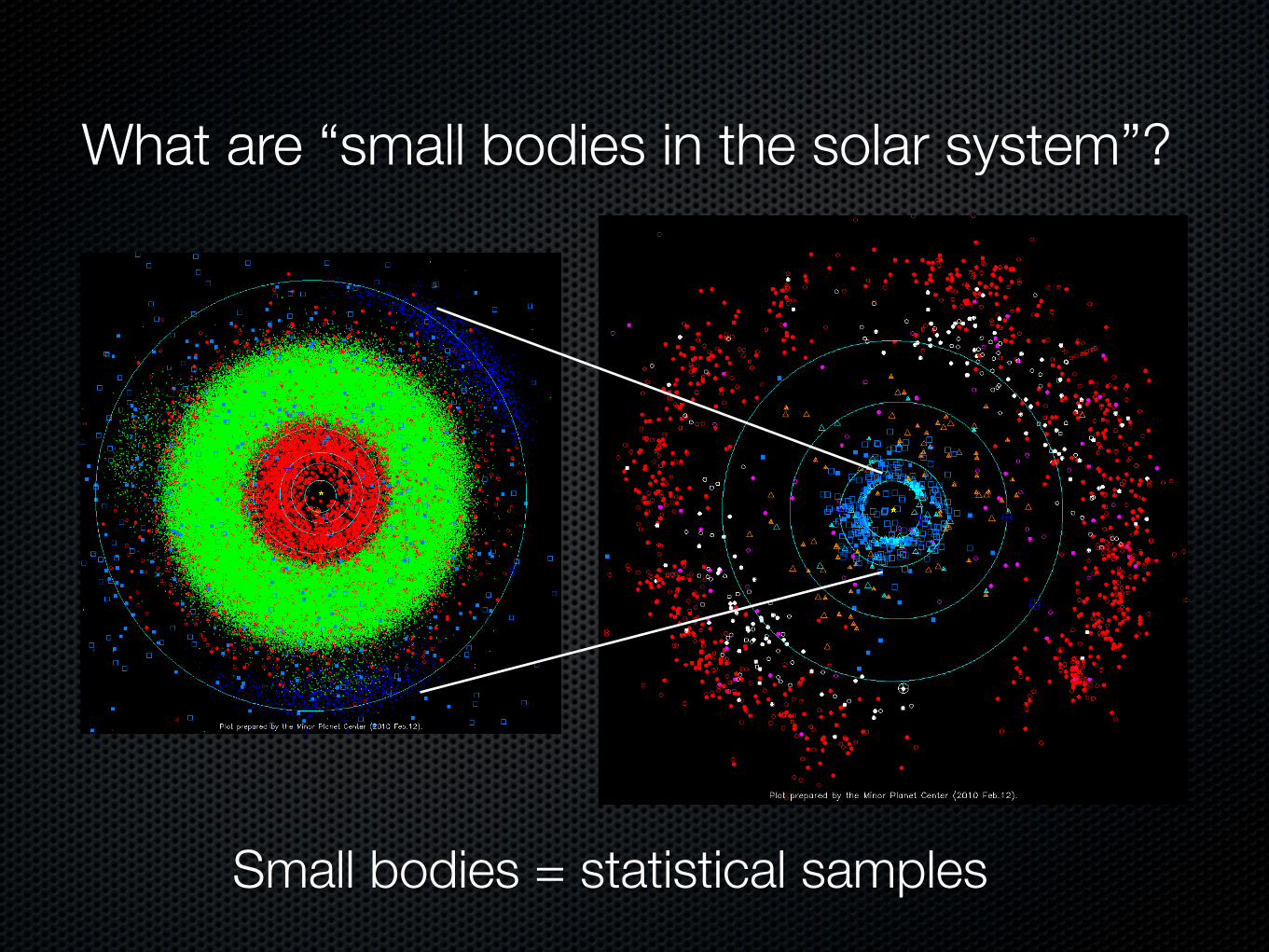
What are “small bodies in the solar system”?

Small bodies = statistical samples

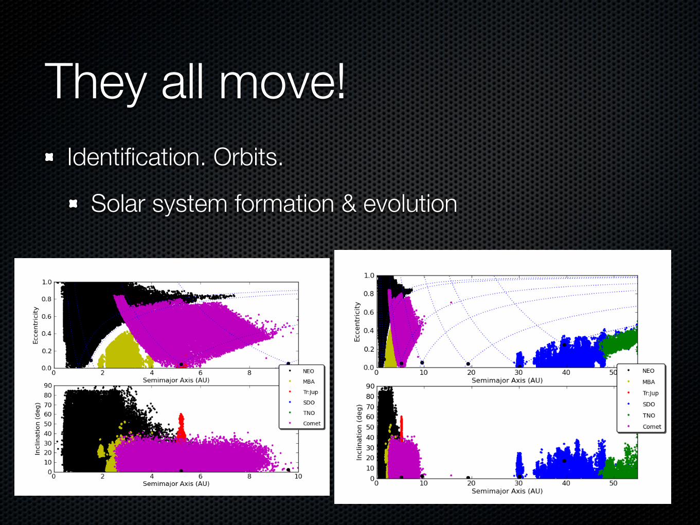
They all move!Identification. Orbits.

Solar system formation & evolution

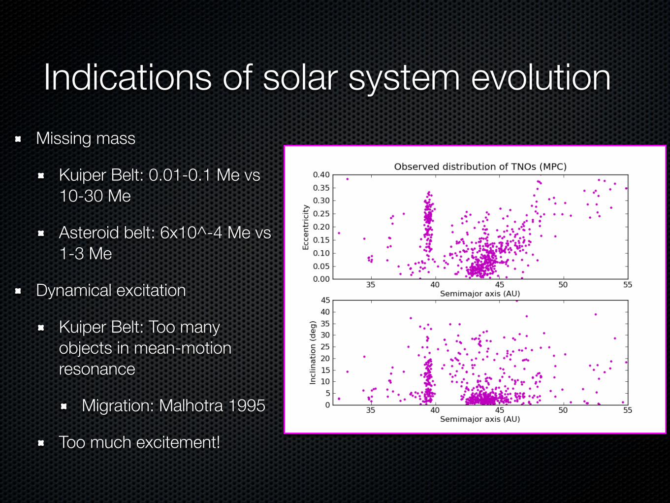
Indications of solar system evolution

Missing mass

Kuiper Belt: 0.01-0.1 Me vs 10-30 Me

Asteroid belt: 6x10^-4 Me vs 1-3 Me

Dynamical excitation

Kuiper Belt: Too many objects in mean-motion resonance

Migration: Malhotra 1995

Too much excitement!

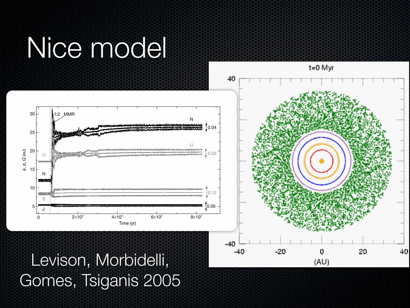
Nice model

Origin of the orbital architecture of the giantplanets of the Solar SystemK. Tsiganis1, R. Gomes1,2, A. Morbidelli1 & H. F. Levison1,3

Planetary formation theories1,2 suggest that the giant planetsformed on circular and coplanar orbits. The eccentricities ofJupiter, Saturn and Uranus, however, reach values of 6 per cent,9 per cent and 8 per cent, respectively. In addition, the inclinationsof the orbital planes of Saturn, Uranus and Neptune take maxi-mum values of,2 degrees with respect to the mean orbital planeof Jupiter. Existing models for the excitation of the eccentricity ofextrasolar giant planets3–5 have not been successfully applied to theSolar System. Here we show that a planetary system with initialquasi-circular, coplanar orbits would have evolved to the currentorbital configuration, provided that Jupiter and Saturn crossedtheir 1:2 orbital resonance. We show that this resonance crossingcould have occurred as the giant planets migrated owing to theirinteraction with a disk of planetesimals6,7. Our model reproducesall the important characteristics of the giant planets’ orbits,namely their final semimajor axes, eccentricities and mutualinclinations.The planetary migration discussed above is a natural result of

planet formation. After the giant planets were formed and thecircumsolar gaseous nebula was dissipated, the Solar System wascomposed of the Sun, the planets and a debris disk of small

planetesimals. The planets then started to erode the disk, by eitheraccreting or scattering away the planetesimals. The planets migratedbecause of the exchange of angular momentum with the diskparticles during this process6,7. Numerical simulations8 show thatJupiter was forced to move inward, while Saturn, Uranus andNeptune drifted outward. The orbital distribution of trans-neptunian objects is probably the result of such planetarymigration7,and suggests that Neptune probably started migrating well inside 20AU while the disk was extended up to 30–35 AU (refs 9–11).Duringmigration, the eccentricities andmutual inclinations of the

planets are damped because of their gravitational interactionwith thedisk particles, in a process known as dynamical friction12. However,the planets’ orbital periods also change. If initially the planets’ orbitswere sufficiently close to each other, it is likely that they had to passthrough low-order mean motion resonances (MMRs), which occurwhen the ratio between two orbital periods is equal to a ratio of smallintegers. These resonance crossings could have excited the orbitaleccentricities of the resonance crossing planets. We focus ourinvestigation on the 1:2 MMR between Jupiter and Saturn, as it isthe strongest resonance.In all our simulations, we started with a system where the initial

LETTERS

Figure 1 | Orbital evolution of the giant planets. These are taken from aN-body simulation with 35ME ‘hot’ disk composed of 3,500 particles andtruncated at 30 AU. Three curves are plotted for each planet: the semimajoraxis (a) and the minimum (q) and maximum (Q) heliocentric distances. U,Uranus; N, Neptune; S, Saturn, J, Jupiter. The separation between the upperand lower curves for each planet is indicative of the eccentricity of the orbit.The maximum eccentricity of each orbit, computed over the last 2Myr of

evolution, is noted on the plot. The vertical dotted line marks the epoch of1:2 MMR crossing. After this point, curves belonging to different planetsbegin to cross, which means that the planets encounter each other. Duringthis phase, the eccentricities of Uranus and Neptune can exceed 0.5. In thisrun, the two ice giants exchange orbits. This occurred in ,50% of oursimulations.

1Observatoire de la Cote d’ Azur, CNRS, BP 4229, 06304 Nice Cedex 4, France. 2GEA/OV/UFRJ and ON/MCT, Ladeira do Pedro Antonio, 43-Centro 20.080-090, Rio deJaneiro, RJ, Brazil. 3Department of Space Studies, Southwest Research Institute, 1050 Walnut Street, Suite 400, Boulder, Colorado 80302, USA.

Vol 435|26 May 2005|doi:10.1038/nature03539

459©!!""#!Nature Publishing Group!

!

Levison, Morbidelli, Gomes, Tsiganis 2005

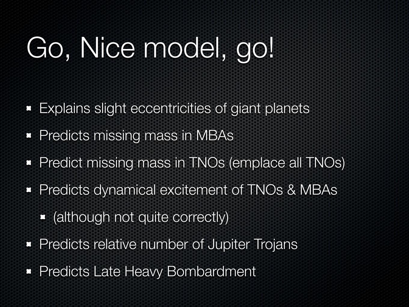
Go, Nice model, go!

Explains slight eccentricities of giant planets

Predicts missing mass in MBAs

Predict missing mass in TNOs (emplace all TNOs)

Predicts dynamical excitement of TNOs & MBAs

(although not quite correctly)

Predicts relative number of Jupiter Trojans

Predicts Late Heavy Bombardment

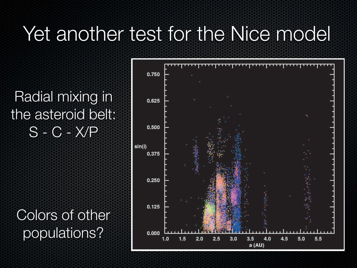
Yet another test for the Nice model

using both the orbital elements and colors. For example,the SDSS colors show that the asteroids with(a, sin i) ! (2.65, 0.20) are distinctively blue (Fig. 3), prov-ing that they do not belong to the family with(a, sin i) ! (2.60, 0.23) but instead are a family in their ownright. While this and several similar examples were alreadyrecognized as clusters in the orbital parameter space (Z95),this work provides a dramatic independent confirmation.Figures 3, 4, and 5 suggest that the asteroid population isdominated by families: even objects that do not belong tothe most populous families, and thus are interpreted asbackground objects in dynamical studies, seem to showcolor clustering. Using the definitions of families based ondynamical analysis (Z95), and aided by SDSS colors, weestimate that at least 90% of asteroids are associated withfamilies.10

Proper orbital elements (MK92) are not available forasteroids with large semimajor axis and orbital inclination.In order to examine the color distribution for objects withlarge semimajor axis, such as Trojan asteroids (a ! 5.2),and for objects with large inclination, such as asteroids fromthe Hungaria family (a ! 1.9, sin i ! 0.38), we use osculat-ing orbital elements. Figure 6 shows the distribution of all

the 10,592 known asteroids observed by SDSS in the spacespanned by osculating semimajor axis and the sine of theorbital inclination angle, with the points color-coded as inFigure 2. It is remarkable that various families can still beeasily recognized thanks to SDSS color information. Thisfigure vividly demonstrates that the asteroid population isdominated by objects that belong to numerous asteroidfamilies.

We are grateful to E. Bowell for making his ASTORB filepublicly available, and to A. Milani, Z. Knezevic, and theircollaborators for generating and distributing proper orbitalelements. We thank Princeton University for generousfinancial support of this research, and M. Strauss andD. Schneider for helpful comments. The Sloan Digital SkySurvey is a joint project of theUniversity of Chicago, Fermi-lab, theInstitute forAdvancedStudy, theJapanParticipationGroup, Johns Hopkins University, the Max-Planck-Institutfur Astronomie, the Max-Planck-Institut fur Astrophysik,NewMexico State University, Princeton University, the USNaval Observatory, and the University of Washington.Apache Point Observatory, site of the SDSS telescopes, isoperated by the Astrophysical Research Consortium. Fund-ing for the project has been provided by the Alfred P. SloanFoundation, the SDSS member institutions, the NationalAeronautics andSpaceAdministration, theNational ScienceFoundation, the US Department of Energy, the JapaneseMonbukagakusho, and the Max-Planck-Gesellschaft. TheSDSSWebsite ishttp://www.sdss.org/.

Fig. 6.—Distribution of 10,592 known asteroids observed by SDSS in the space spanned by the osculating inclination and semimajor axis. The dots are col-ored according to their position in SDSS color-color diagram shown in Fig. 2. Note that the asteroid population is dominated by families.

10 The preliminary analysis indicates that about 1%–5% of objects donot belong to families. A more detailed discussion of the robustness of thisresult will be presented in a forthcoming publication. Similarly, it is not cer-tain yet whether objects not associated with the families show any heliocen-tric color gradient.

ASTEROID FAMILIES 2947

Radial mixing in the asteroid belt:

S - C - X/P

Colors of other populations?

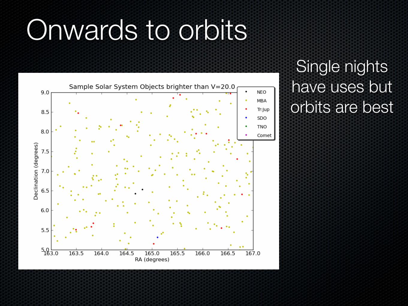
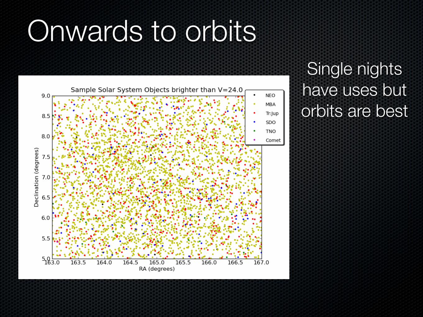
Onwards to orbitsSingle nights have uses but orbits are best

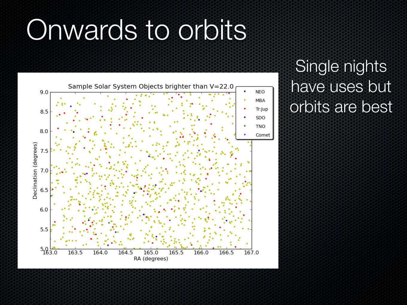
Onwards to orbitsSingle nights have uses but orbits are best

Onwards to orbitsSingle nights have uses but orbits are best

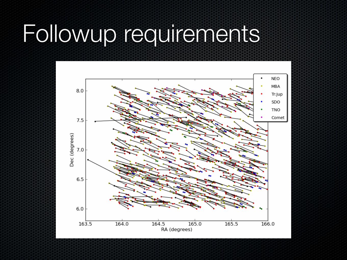
Followup requirements

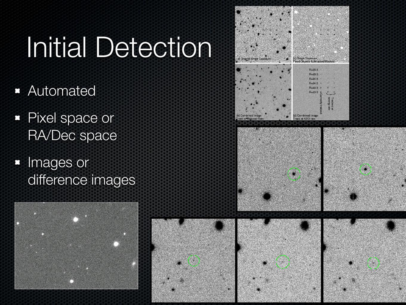
Initial DetectionAutomated

Pixel space or RA/Dec space

Images or difference images

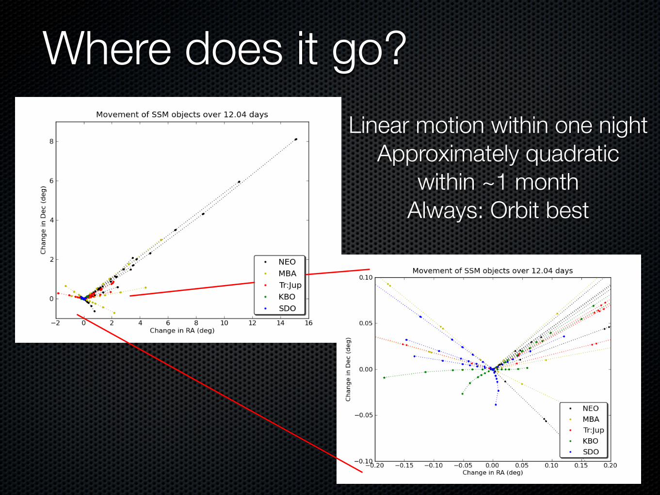
Where does it go?

Linear motion within one nightApproximately quadratic

within ~1 monthAlways: Orbit best

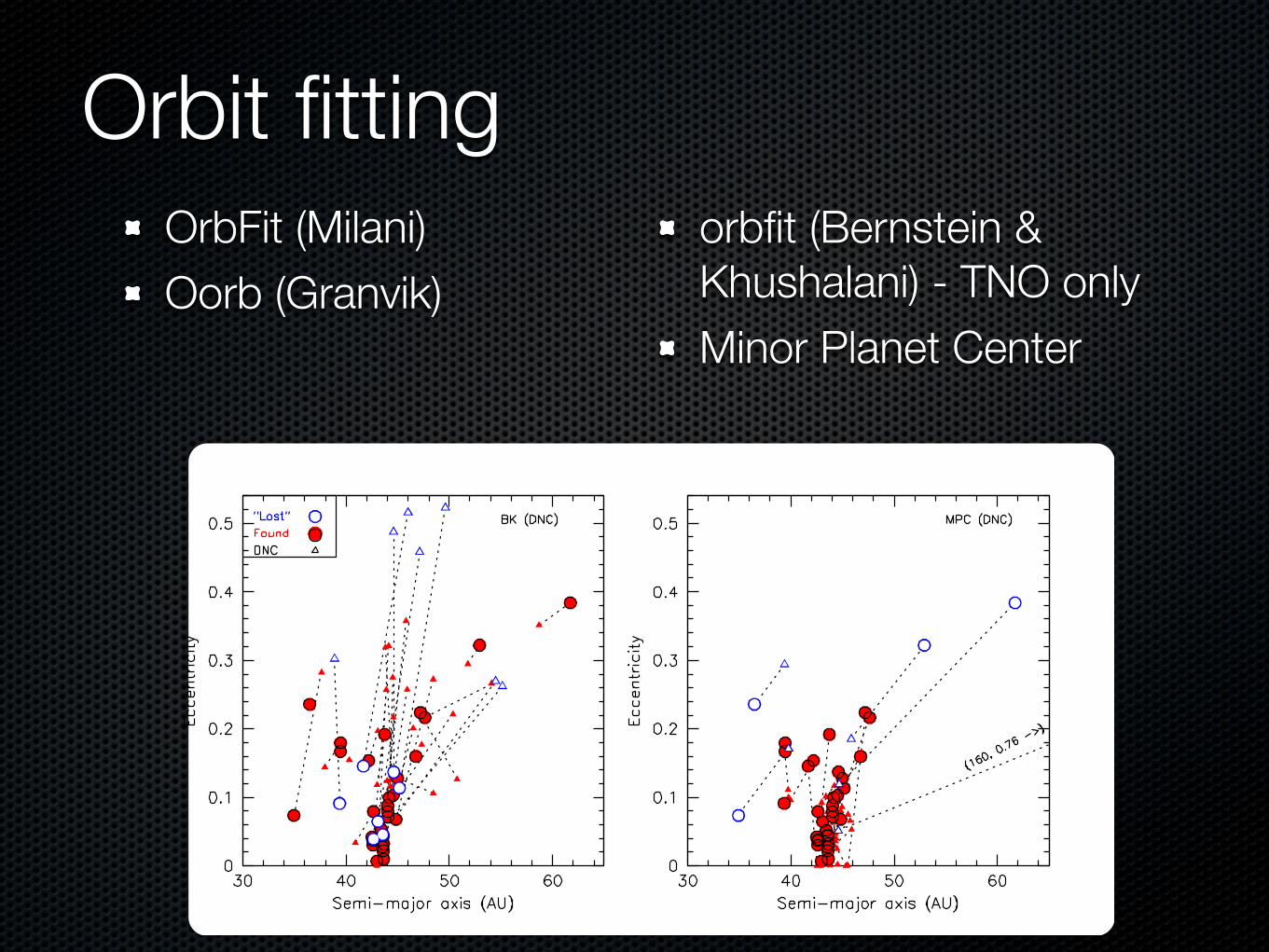
Orbit fittingOrbFit (Milani)Oorb (Granvik)

orbfit (Bernstein & Khushalani) - TNO onlyMinor Planet Center

Some recent surveys for further references

NEOs - Catalina Sky Survey

Asteroids - SDSS (Ivezic etal 2001). “SKADS” (Gladman etal 2009)

Trojans (Jupiter) - SDSS (Szabo etal 2007)

TNOs - “DES” (Millis etal 2002). “CFEPS” (Kavelaars 2009).

Conclusions

Finding moving objects, linking them into orbits can be tough

Biases can creep in everywhere (initial selection, linking, orbit fitting, followup)

What you learn from orbits (and physical properties if you get that bonus) is worth it - planetary formation and evolution!