IZA DP No. 3334

Outsourcing and Technological Innovations:A Firm-Level Analysis

Ann BartelSaul LachNachum Sicherman

DI

SC

US

SI

ON

PA

PE

R S

ER

IE

S

Forschungsinstitutzur Zukunft der ArbeitInstitute for the Studyof Labor

February 2008

Outsourcing and Technological

Innovations: A Firm-Level Analysis

Ann Bartel Columbia University and NBER

Saul Lach

Hebrew University and CEPR

Nachum Sicherman Columbia University and IZA

Discussion Paper No. 3334 February 2008

IZA

P.O. Box 7240 53072 Bonn

Germany

Phone: +49-228-3894-0 Fax: +49-228-3894-180

E-mail: iza@iza.org

Any opinions expressed here are those of the author(s) and not those of IZA. Research published in this series may include views on policy, but the institute itself takes no institutional policy positions. The Institute for the Study of Labor (IZA) in Bonn is a local and virtual international research center and a place of communication between science, politics and business. IZA is an independent nonprofit organization supported by Deutsche Post World Net. The center is associated with the University of Bonn and offers a stimulating research environment through its international network, workshops and conferences, data service, project support, research visits and doctoral program. IZA engages in (i) original and internationally competitive research in all fields of labor economics, (ii) development of policy concepts, and (iii) dissemination of research results and concepts to the interested public. IZA Discussion Papers often represent preliminary work and are circulated to encourage discussion. Citation of such a paper should account for its provisional character. A revised version may be available directly from the author.

IZA Discussion Paper No. 3334 February 2008

ABSTRACT

Outsourcing and Technological Innovations: A Firm-Level Analysis*

This paper presents a dynamic model that analyzes how firms’ expectations with regards to technological change influence the demand for outsourcing. We show that outsourcing becomes more beneficial to the firm when technology is changing rapidly. As the pace of innovations in production technology increases, the firm has less time to amortize the sunk costs associated with purchasing the new technologies. This makes producing in-house with the latest technologies relatively more expensive than outsourcing. The model therefore provides an explanation for the recent increases in outsourcing that have taken place in an environment of increased expectations for technological change. We test the predictions of the model using a panel dataset on Spanish firms for the period 1990 through 2002. The empirical results support the main prediction of the model, namely, that all other things equal, the demand for outsourcing increases with the probability of technological change. JEL Classification: O33, L24, L11, J21 Keywords: technological change, outsourcing Corresponding author: Nachum Sicherman Graduate School of Business Columbia University New York, NY 10027 USA E-mail: Nachum.Sicherman@Columbia.edu

* The authors gratefully acknowledge the generous support of grants from the Columbia University Institute for Social and Economic Research and Policy and the Columbia Business School’s Center for International Business Education and Research and outstanding research assistance from Ricardo Correa and Cecilia Machado. Saul Lach acknowledges the support of the European Commission grant CIT5-CT-2006-028942

I. Introduction

Outsourcing, or the contracting out of activities to subcontractors outside the firm,

has become more widespread in recent decades. For example, Magnani (2006) reports

that the cost share of purchased services in U.S. manufacturing industries grew from

4.4% in 1949 to 12% in 1998. Similar increases in outsourcing have been observed in

Europe as well.1 A large theoretical literature has examined the determinants of the

decision to outsource, or, more generally, the organization of production. Outsourcing

parts of the production of a final product is costly because of the costs associated with

searching and finding an appropriate input supplier and, more importantly, because

contracting with outside suppliers may be imperfect if some attributes of the outsourced

inputs are not verifiable by third parties. This limits contracting possibilities and creates a

potential hold-up problem.2 These ideas go back to Williamson (1975, 1985) and

Grossman and Hart (1986) and have been recently incorporated into industry equilibrium

models by Grossman and Helpman (2002) while their implications for international trade

are analyzed in Antras and Helpman (2004).

In this paper we present a dynamic model that analyzes how firms’ expectations

with regards to technological change influences the demand for outsourcing – an issue

not addressed in previous models – while abstracting from other considerations (e.g.,

transaction costs, specificity, etc.). We show that outsourcing becomes more beneficial to

the firm when technology is changing rapidly. A firm can buy the latest technology and

1 See Arndt and Kierzkowski (2001), Mol (2005) and Abramovsky and Griffith (2006). 2 Baker and Hubbard (2003) consider how information technology in the trucking industry impacts contracting possibilities and vertical integration. Baccara (2007) uses a general equilibrium model to study how information leakages could affect a firm’s outsourcing decision as well as its investments in R&D.

2

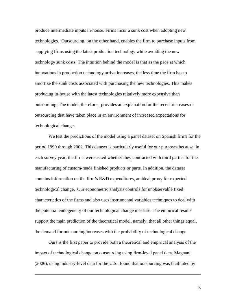
produce intermediate inputs in-house. Firms incur a sunk cost when adopting new

technologies. Outsourcing, on the other hand, enables the firm to purchase inputs from

supplying firms using the latest production technology while avoiding the new

technology sunk costs. The intuition behind the model is that as the pace at which

innovations in production technology arrive increases, the less time the firm has to

amortize the sunk costs associated with purchasing the new technologies. This makes

producing in-house with the latest technologies relatively more expensive than

outsourcing, The model, therefore, provides an explanation for the recent increases in

outsourcing that have taken place in an environment of increased expectations for

technological change.

We test the predictions of the model using a panel dataset on Spanish firms for the

period 1990 through 2002. This dataset is particularly useful for our purposes because, in

each survey year, the firms were asked whether they contracted with third parties for the

manufacturing of custom-made finished products or parts. In addition, the dataset

contains information on the firm’s R&D expenditures, an ideal proxy for expected

technological change. Our econometric analysis controls for unobservable fixed

characteristics of the firms and also uses instrumental variables techniques to deal with

the potential endogeneity of our technological change measure. The empirical results

support the main prediction of the theoretical model, namely, that all other things equal,

the demand for outsourcing increases with the probability of technological change.

Ours is the first paper to provide both a theoretical and empirical analysis of the

impact of technological change on outsourcing using firm-level panel data. Magnani

(2006), using industry-level data for the U.S., found that outsourcing was facilitated by

3

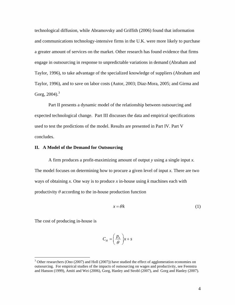
technological diffusion, while Abramovsky and Griffith (2006) found that information

and communications technology-intensive firms in the U.K. were more likely to purchase

a greater amount of services on the market. Other research has found evidence that firms

engage in outsourcing in response to unpredictable variations in demand (Abraham and

Taylor, 1996), to take advantage of the specialized knowledge of suppliers (Abraham and

Taylor, 1996), and to save on labor costs (Autor, 2003; Diaz-Mora, 2005; and Girma and

Gorg, 2004).3

Part II presents a dynamic model of the relationship between outsourcing and

expected technological change. Part III discusses the data and empirical specifications

used to test the predictions of the model. Results are presented in Part IV. Part V

concludes.

II. A Model of the Demand for Outsourcing

A firm produces a profit-maximizing amount of output y using a single input x.

The model focuses on determining how to procure a given level of input x. There are two

ways of obtaining x. One way is to produce x in-house using k machines each with

productivity θ according to the in-house production function

x kθ= (1)

The cost of producing in-house is

kH

pC xθ

⎛ ⎞ s= +⎜ ⎟⎝ ⎠

3 Other researchers (Ono (2007) and Holl (2007)) have studied the effect of agglomeration economies on outsourcing. For empirical studies of the impacts of outsourcing on wages and productivity, see Feenstra and Hanson (1999), Amiti and Wei (2006), Gorg, Hanley and Strobl (2007), and Gorg and Hanley (2007).

4

where pk is the (rental) price of a machine and s is a sunk cost associated with installing

and using the machines of a given productivity (or vintage) for the first time. s is

incurred only once. This initial installation cost also reflects training costs.

The second way of procuring x is to buy it in the market. We call this outsourcing

production. The cost of this alternative is

OC px=

where p is the unit price of x.

We assume that outsourcing costs are the same across firms, but allow for

heterogeneity in the sunk cost of in-house production by assuming that s is distributed

among firms with distribution G(s).

Assuming constant returns to scale in production we can, without loss of

generality, set x = y and write the costs as functions of y (which is observable)

kH

O

pC y

C pyθ

⎛ ⎞ s= +⎜ ⎟⎝ ⎠

= (2)

As in Ono (2000), the firm chooses the procuring alternative that minimizes costs.

Let 1χ = indicate a firm that outsources its production.4 This simple model implies

)

4 The constant returns to scale assumption implies that the firm either produces all y in-house or outsources all of y, therefore it is not optimal to split a given level of y between in-house and outsourcing.

The cost of splitting y between in-house ( Hy and outsourcing is ( )Oy ( ) ,kpO Hpy yθ s+ + where

We can write this cost as .O Hy y y= + ( ) .kpHpy p y sθ− − + It follows that producing all of y in-

house minimizes costs when kpp θ> , i.e., when outsourcing is expensive, and, conversely, outsourcing

5

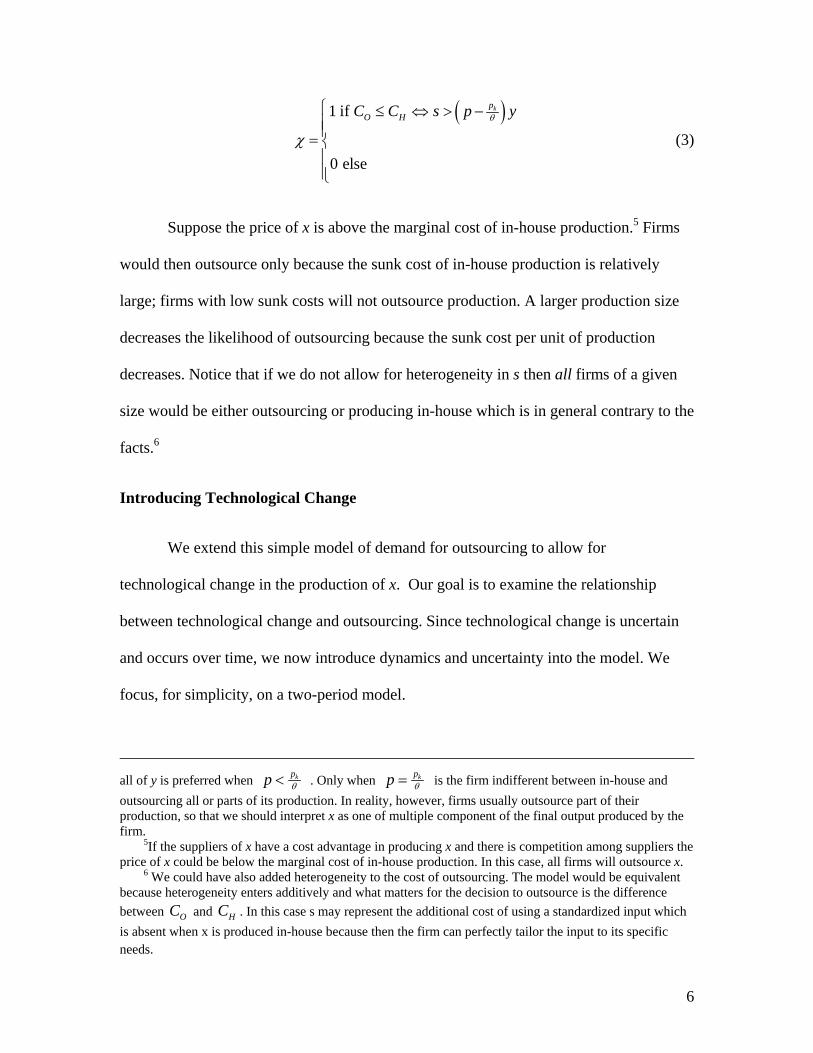
( )1 if

0 else

kpO HC C s p yθ

χ

⎧ ≤ ⇔ > −⎪⎪= ⎨⎪⎪⎩

(3)

Suppose the price of x is above the marginal cost of in-house production.5 Firms

would then outsource only because the sunk cost of in-house production is relatively

large; firms with low sunk costs will not outsource production. A larger production size

decreases the likelihood of outsourcing because the sunk cost per unit of production

decreases. Notice that if we do not allow for heterogeneity in s then all firms of a given

size would be either outsourcing or producing in-house which is in general contrary to the

facts.6

Introducing Technological Change

We extend this simple model of demand for outsourcing to allow for

technological change in the production of x. Our goal is to examine the relationship

between technological change and outsourcing. Since technological change is uncertain

and occurs over time, we now introduce dynamics and uncertainty into the model. We

focus, for simplicity, on a two-period model.

kpp θ< kpp θ=all of y is preferred when . Only when is the firm indifferent between in-house and

outsourcing all or parts of its production. In reality, however, firms usually outsource part of their production, so that we should interpret x as one of multiple component of the final output produced by the firm.

5If the suppliers of x have a cost advantage in producing x and there is competition among suppliers the price of x could be below the marginal cost of in-house production. In this case, all firms will outsource x.

6 We could have also added heterogeneity to the cost of outsourcing. The model would be equivalent because heterogeneity enters additively and what matters for the decision to outsource is the difference between and OC HC . In this case s may represent the additional cost of using a standardized input which is absent when x is produced in-house because then the firm can perfectly tailor the input to its specific needs.

6

Suppose that technology (i.e., the productivity of machines) in the first period is given by

1.θ In the second period, productivity can either increase to 2 2 1, ,θ θ θ> with probability

λ or remain at 1θ with the complementary probability, i.e.,

2

1

with probability

with probability 1

θ λθ

θ λ

⎧⎪= ⎨⎪ −⎩

At the beginning of each period, the firm decides to outsource or to produce in-

house given the observed technology level and prices. We denote the price of x in period

1 by 1.p We assume that x is supplied by firms using the latest technologies. As

production technology improves, firms can charge a lower price of x and still make

profits. Whether they will do this or not depends on the competitive environment. We do

not model the supply side here but allow the price of x to change as technology improves.

We let p2 be the price of x when a technological change occurs in the second period,

and p2 be the price of x when technology does not change. Because the price of

machines does not change, their quality-adjusted price kpθ declines as technology

improves.

We proceed backwards. Suppose there is technological change in the second

period. The firm faces three alternatives: it can outsource, it can produce in-house with

the old technology or it can pay the sunk cost and upgrade to the new vintage of

machines. To simplify the analysis we make the assumption that upgrading always

dominates keeping the old technology. This requires a not too large sunk cost, namely

( )2 1

1 2,ks p y θ θ

θ θ−≤ which we assume to hold, i.e.,

7

⎟⎟⎠

⎞⎜⎜⎝

⎛ −≥=

12

121)(θθθθ

ypsforsG k (4)

In this case, the firm’s decision is essentially as in the static model analyzed in the

previous section: to outsource or to produce in-house. Because producing in-house

requires incurring the sunk cost, the firm’s decision in the first period does not affect its

current decision. Then, as in (3), when there is a technological improvement, the demand

for outsourcing is

( )22

2

1 if

0 else

kps p yλ θ

χ

⎧ ≥ −⎪⎪= ⎨⎪⎪⎩

(5)

If there is no technological change, the firm’s decision depends on its outsourcing

decision in the first period. If the firm produced in-house in the first period, it already

paid the sunk cost s for the use of the technology and therefore it will outsource only if

1 2 .kp y p yθ > But, if the firm outsourced in the first period, the cost of using the old

technology in-house is 1

kp y sθ + which needs to be compared to the cost of outsourcing,

2 .p y This gives the following outsourcing decision in period 2 in the absence of

technological change,

( )11 2

2

1 if

0 else

kps p yθχ

χ

⎧ × ≥ −⎪⎪= ⎨⎪⎪⎩

(6)

Because of the presence of sunk costs, the decision to outsource during the first

period affects future decisions if technological change does not occur. Specifically, a firm

8

that did not outsource during the first period, 1 0,χ = will be less likely to outsource

during the second period if no technological change occurs.

In the first period, the firm chooses to outsource or produce in-house by

comparing the expected discounted costs of each alternative. These costs are,

1 1 2 21 2

1 21 1

( 1) (1 ) , ,

( 0) (1 ) , ,

k k

k k

p pC p y Min p y y s Min p y y

p pC y s Min p y y Min p y

λ

λ

χ β λ βλθ θ

χ β λ βλθ θ 2

2

k

s

p y sθ

⎧ ⎫ ⎧= = + − + + +

⎫⎨ ⎬ ⎨⎩ ⎭ ⎩

⎬⎭

⎧ ⎫ ⎧= = + + − + +

⎫⎨ ⎬ ⎨⎩ ⎭ ⎩

⎬⎭

where β is the discount factor.

The difference between these two costs is

( )1 1 11

2 21 1

( 1) ( 0) 1 (1 )

(1 ) ,0 (1 ) ,0

k

k k

pC C p y s

p pMin p y s Min p y

χ χ β λθ

β λ β λθ θ

⎛ ⎞= − = = − − − − +⎜ ⎟

⎝ ⎠⎧ ⎫ ⎧⎛ ⎞ ⎛ ⎞⎪ ⎪ ⎪− − − − − −⎨ ⎬ ⎨⎜ ⎟ ⎜ ⎟⎪ ⎪ ⎪⎝ ⎠ ⎝ ⎠⎩ ⎭ ⎩

⎫⎪⎬⎪⎭

which can be written as,

( ) ( )

( ) ( ) ( )

( ) ( ) ( )

1 1

1 1

1 1

1 2

1 1 1 2 2

1 2

0

( 1) ( 0) (1 ) , 0

1 (1 ) ,

k k

k k

k k

p p

p p

p p

p y s p y

C C p y p y s p y

p y s p y s

θ θ

θ θ

θ θ

χ χ β λ

β λ

⎧ − − − ≤⎪⎪⎪⎪= − = = − + − − − ≤ − ≤⎨⎪⎪⎪ − − − − − ≥⎪⎩

1

kp sθ (7)

We can rule out the first case because it is reasonable to assume that the price of x

in period 2 (the last period) cannot be below the marginal cost of in-house production,

9

i.e.,7

21

kppθ

≥ (8)

The firm decides to outsource in the first period whenever 1 1( 1) ( 0) 0.C Cχ χ= − = <

The decision to outsource in the first period therefore depends on current and future

prices of x as well as on the size of sunk costs and the probability of technological change

,

( ) ( ) ( )

( ) ( )

1 1

1 1

1

1 2

121 (1 )

1 if (1 ) and

1 if and

0 else

k k

pkk

p p

p y p

s p y p y s p y

s s p yθ

θ θ

β λ θ

β λ

χ −

− −

⎧ ≥ − + − − ≥ −⎪⎪⎪

= ⎨ ≥ ≤ −⎪⎪⎪⎩

12kp

θ

(9)

From (7) we see that, all other things equal, an increase in λ decreases the cost of

outsourcing relative to that of in-house production making the firm more likely to decide

to outsource in the first period. This is the main message of the model: when the

likelihood of technological change increases, firms will be more reluctant to purchase the

technology to produce in-house because it will soon be obsolete. Upgrading the

technology involves incurring a sunk cost “di novo.” The more frequent the innovations

arrive, the less time the firm has to amortize these sunk costs. The firm can use

outsourcing to obtain x from supplying firms using the latest technology and avoid the

sunk costs.

7This assumption depends on the type of technology and competition among the firms producing x.

10

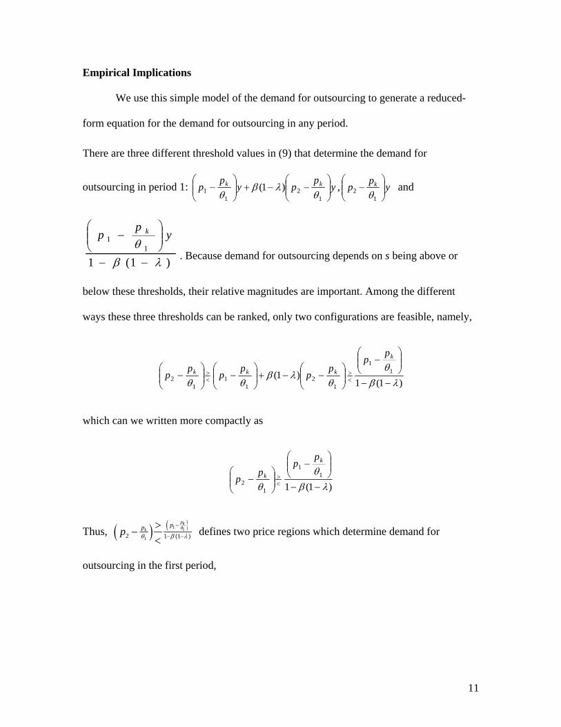
Empirical Implications

We use this simple model of the demand for outsourcing to generate a reduced-

form equation for the demand for outsourcing in any period.

There are three different threshold values in (9) that determine the demand for

outsourcing in period 1: yp

pyp

p kk⎟⎟⎠

⎞⎜⎜⎝

⎛−−+⎟⎟

⎠

⎞⎜⎜⎝

⎛−

12

11 )1(

θλβ

θ, ypp k

⎟⎟⎠

⎞⎜⎜⎝

⎛−

12 θ

and

)1(11

1

λβθ−−

⎟⎟⎠

⎞⎜⎜⎝

⎛− y

pp k

. Because demand for outsourcing depends on s being above or

below these thresholds, their relative magnitudes are important. Among the different

ways these three thresholds can be ranked, only two configurations are feasible, namely,

)1(1)1( 1

1

12

11

12 λβ

θθ

λβθθ −−

⎟⎟⎠

⎞⎜⎜⎝

⎛−

⎟⎟⎠

⎞⎜⎜⎝

⎛−−+⎟⎟

⎠

⎞⎜⎜⎝

⎛−⎟⎟

⎠

⎞⎜⎜⎝

⎛− <

><>

k

kkk

pp

pp

pp

pp

which can we written more compactly as

)1(11

1

12 λβ

θθ −−

⎟⎟⎠

⎞⎜⎜⎝

⎛−

⎟⎟⎠

⎞⎜⎜⎝

⎛− <

>

k

k

pp

pp

Thus, ( ) ( )1 1

12 1 (1 )

pkk

ppp θ

θ β λ

−

− −

>−

< defines two price regions which determine demand for

outsourcing in the first period,

11

( ) ( ) ( )

( ) ( ) ( ) ( )

1 11 1

1

1 1

1 1 1

21 (1 ) 1 (1 )

11 2 2 1 (1 )

1 if when

1 if (1 ) when

0 else

p pk kk

pkk k k

p y p yp

p yp p p

s p y

s p y p y p y

θ θ

θ

β λ θ β λ

θ θ θ β λ

χβ λ

− −

− − − −

−

− −

⎧ ≥ − ≥⎪⎪⎪⎪= ⎨ ≥ − + − − − ≤⎪⎪⎪⎪⎩

which implies

( ) ( ) ( )

( ) ( )( ) ( ) ( )

1 11 1

1

1 1

1 1 1

21 (1 ) 1 (1 )

1

1 2 2 1 (1 )

1 when

( )

1 (1 ) when

θ θ

θ

β λ θ β λ

θ θ θ β λ

χ

β λ

− −

− − − −

−

− −

⎧ ⎛ ⎞− − ≥⎜ ⎟⎪ ⎝ ⎠⎪⎪= ⎨⎪⎪ − − + − − − ≤⎪⎩

p pk kk

pkk k k

p pp

pp p p

G y p

E

G p y p y p

Notice that, for given prices, 1 (G )− ⋅ increases with λ so that the demand for

outsourcing in period 1 is increasing in the probability of technological change λ.

The demand for outsourcing in period 2 is given by

( ) ( )( ) ( ) ( )( )

2 2 2

2 2 1 1 2 2 1 1

| 1

1 | 0, 1 ( ) | 0, 0 1 ( )

E E T

E T E E T E

χ λ χ

λ χ χ χ χ χ χ

= =

+ − = = + = = −⎡ ⎤⎣ ⎦

where T2 is an indicator for technological change occurring in period 2.

In this simple model, ( 2 2 1| 0, 0E Tχ χ ) 0= = = because a firm that did not

outsource in the first period will continue producing in-house in the second period if θ

does not change. Expected outsourcing demand in the second period is therefore

( ) ( )2 2 22 1

1 1 1k kp pE G p y G p yλ 1( )Eχ λ λθ θ

⎡ ⎤ ⎡⎛ ⎞ ⎛ ⎞⎛ ⎞ ⎛ ⎞= − − + − − −⎢ ⎥ ⎢⎜ ⎟ ⎜ ⎟⎜ ⎟ ⎜ ⎟⎜ ⎟ ⎜ ⎟⎢ ⎥ ⎢⎝ ⎠ ⎝ ⎠⎝ ⎠ ⎝ ⎠⎣ ⎦ ⎣

χ⎤⎥⎥⎦

(10)

12

Given prices, 2( )E χ is an increasing function of λ when the price margin after

an innovation occurs, 22 ,kpp λ θ− is no larger than the price margin when there is no

technology change, 12 .kpp θ− This sufficient condition is likely to hold under many

market structures because the number of potential outsourcers is larger after an

innovation occurs prompting supplying firms to lower their markups in order to capture a

larger market share.

III. Data and Empirical Specification

We use the Encuesta sobre Estrategias Empresariales (ESEE, or Survey on

Business Strategies), a panel of approximately 1800 Spanish manufacturing companies,

surveyed annually since 1990. Data are currently available through 2002. The survey is

conducted by the Fundacion SEPI with the support of the Ministry of Industry, Tourism

and Trade. We use data from the 1990, 1994, 1998 and 2002 surveys.8

In each survey, the firms were asked if they contracted with third parties for the

manufacture of custom-made finished products or parts, and if so, the value of the

outsourced products or parts. We use this information to create two indicators of

outsourcing, a dummy for whether or not the firm did engage in outsourcing, and the

value of outsourcing divided by total costs.9 Table 1 shows, by industry sector and

overall, the percentage of firms that reported outsourcing at least some part of production

during the 1990–2002 time period and the mean value of the outsourced production as a

8 Budgetary constraints prevented us from purchasing data for all of the years between 1990 and 2002. 9 Lopez (2002) describes the evolution of outsourcing of services and of production in Spanish manufacturing firms using a sub-sample of the ESSE data for the period 1990-1999. He finds significant differences in outsourcing between small and large firms and a positive effect of outsourcing on productivity.

13

percentage of total cost. On average, 41% of firms reported that they outsourced

production during this time period. The outsourcing percentage rose from 35% in 1990 to

43% in 2002. There is significant variation in the likelihood of outsourcing across

industries ranging from a low of 16% for Drinks to a high of 61% for Machinery and

Mechanical Goods. The value of the outsourced production as a percentage of total costs

is approximately 5 percent during this time period; for firms that did outsource

production, the mean value of outsourced production as a percentage of total costs is 11

percent.

In the previous section, we derived the demand for outsourcing in period t as a

function of the probability of technological change, output, and the various input prices

and technology parameters. Notice that the demand function differs between periods 1

and 2 because of the dynamic nature of the problem and the finiteness of the model. We

will ignore this issue in the empirical application because we implicitly assume that the

data-generating process has been going on for some time so that the relationship between

outsourcing and its drivers stabilizes over time. Under the assumption that input prices

and technology parameters are common to all firms in an industry, these can be captured

by industry dummies (ID). Thus,

( ) ( , , )t tE h y IDtχ λ= (11)

Equation (11) is a reduced-form expression because all the arguments in the h function

are exogenous in the model.10 The main implication of the theoretical model is that, all

10Equation (10) is a dynamic equation that could also serve as the basis for estimating the relationship between outsourcing and λ. It is, however, specific to a 2-period model. In a model with 3 or more periods the dynamics are much more complicated. We therefore prefer to estimate reduced form equations.

14

other things equal, the demand for outsourcing increases with the exogenous probability

of technological change λ.

In order to test this implication we need a proxy for λ. We will proxy λ by an

binary variable indicating whether a firm engages in R&D, and if it does, we will also use

the amount of R&D expenditures. The rationale for this proxy is that a firm that engages

in R&D is more likely to experience technological change (new processes and/or new

products) as compared to a firm that does not engage in R&D. Table 1 shows that during

the time period under study, 36 percent of the firms in the sample engaged in R&D, with

this percentage ranging from a low of 13% for Editing and Printing to 67% for

Chemicals.

We make separability and linearity assumptions on the function h,

itj

ijjityitrit uIDyr +++= ∑δββχ (12)

where rit is our measure of R&D (a dummy for being engaged in R&D and/or the ratio of

R&D expenditures to sales) and 1ijID = if firm i is in industry j and zero otherwise. By

using the two measures of rit we are able to study whether the extensive or the intensive

margin of R&D is more important in explaining outsourcing. We will estimate this

equation for all years using clustered standard errors at the firm level to account for

heteroskedasticity and arbitrary serial correlation.

Although the model assumes λ to be exogenous, a serious concern is that the

probability that the firm will experience technological change is determined by

unobserved factors that also affect the decision to outsource. More innovative firms may

15

be doing more R&D and may also be adopting new production methods that require more

outsourcing, i.e., λ, or its R&D proxy, may be endogenous in the outsourcing equation.

The estimated R&D coefficient will therefore not capture the causal effect of

technological change on outsourcing. We address this concern by allowing for a time-

invariant component in uit to affect both the decision to engage in R&D (and therefore λ)

and the decision to outsource, i.e., it i itu µ η= + . Consistent estimates under this

assumption can be obtained from time-differencing equation (12)

( ) ( ) 1111 −−−− −+−+−=− itititityititritit yyrr ηηββχχ (13)

and estimating this equation by OLS period by period. These estimates are consistent

provided R&D is strictly exogenous.

The strict exogeneity assumption is quite strong because it precludes any

correlation between shocks that affected outsourcing in previous periods and current

R&D expenditures. We therefore make a weaker assumption that allows for outsourcing

to affect future R&D expenditures,

0,...),|( 1 =−ititit rrE η (14)

Under this assumption, we can use the lag of R&D as an instrument for in

equation (13) to obtain consistent estimates of the parameters.

1−− itit rr

Equation (12) includes, in addition to the proxy for technological change, the

firm’s annual sales (Sales) as well as a vector of industry dummies. We also add two

variables that measure the firm’s current technological intensity, whether it uses

16

computerized digital machine tools (comp_dmt) or uses robotics (comp_robotic). 11

In order to control for factors other than technological change that may contribute

to outsourcing, we also include a set of variables that have been the focus of previous

research on the determinants of outsourcing. Since firms may use outsourcing as a way of

economizing on labor costs (see Abraham and Taylor, 1996), we include the firm’s

average labor cost defined as total annual spending (wages and benefits) on “staff”

divided by total employment (wage). Outsourcing may also be used to smooth the

workload of the core workforce during peaks of demand (Abraham and Taylor, 1996;

Holl, 2007). Hence, we add a measure of capacity utilization (capacity) defined as the

average percentage of the standard production capacity used during the year. Small firms

would be expected to be more likely to outsource because it may not be optimal for them

to carry out all steps in the production process because of the costs of maintaining

specialized equipment or skills in-house (Abraham and Taylor, 1996). Hence we control

for the size of the firm using four categories for number of employees. Another factor

that can increase the propensity to outsource is the volatility in demand for the product

(Abraham and Taylor, 1996; Holl, 2007). We control for this by adding dummy variables

for whether the main market the company serves expanded (market_expand) or declined

(market_decline) during the year. It has also been argued that older firms are more likely

to outsource because they have had time to learn about the quality and reliability of

potential subcontractors (Holl, 2007). We therefore include the age of the firm (age).

Whether the firm primarily produces standardized products or custom products should

also affect the propensity to outsource with firms focusing on product variety being more

11 These two variables may also be correlated with technological change and their inclusion in the equation

17

likely to outsource some of their production; we therefore add a dummy variable

indicating that the firm produces standardized products that are, in most cases, the same

for all buyers (std_product). Finally, we control for the firm’s export propensity, the

value of its exports divided by its sales (export), and whether the firm has any foreign

ownership (foreign_own). Both of these factors have been included in prior studies of

outsourcing (Girma and Gorg, 2004; Diaz-Mora, 2005; and Holl, 2007).

IV. Results

We estimated Equation (12) using two dependent variables: whether or not the

firm engaged in outsourcing and the value of the firm’s outsourced production as a

percentage of total costs. Results for the first dependent variable are shown in Table 2

and for the second in Table 3. Each table provides the coefficients on the R&D dummy

using various approaches to estimating Equation (12). The coefficients on the other

variables included in these regressions are shown in Appendix Tables A-1 and A-2.

Columns (1), (2) and (3) in Table 2 use OLS, probit and logit, respectively, to

estimate Equation (12). We find remarkably similar results across these three columns;

firms that engage in R&D are 11-12 percent more likely to outsource some part of their

production. When we control for firm-specific time-invariant unobservable factors in

Column (4), firms that engage in R&D are 9.5% more likely to outsource production.

Using first-differences in column (5), the coefficient on R&D falls to 0.066 but is still

very significant. Column (6) adds the R&D/sales ratio and we find that what matters is

whether the firm engages in R&D, not its R&D-intensity. Finally, in column (7), we use

could weaken the measured effect of the R&D variable.

18

the first lag of R&D as an instrument for the growth rate of R&D.12 Although the

coefficient on R&D is no longer significant because of the doubling of the standard error,

the magnitude of the coefficient is virtually identical to the coefficient reported in column

(5).

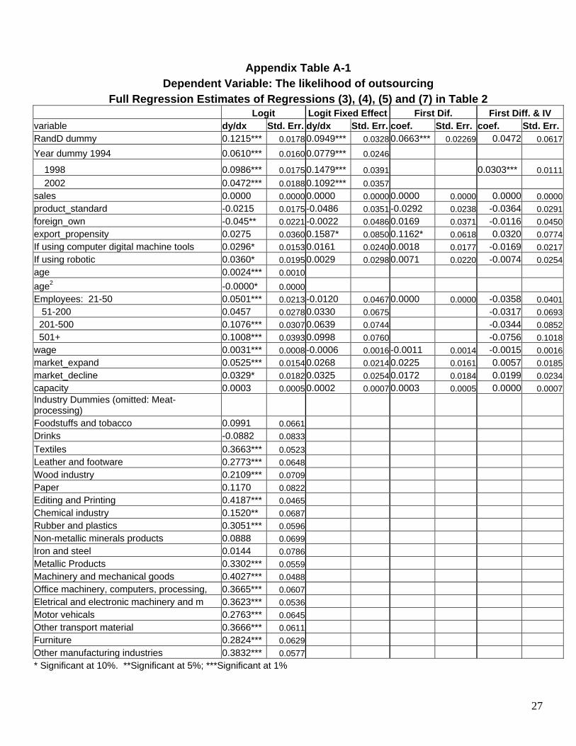
The results in Appendix Table A-1 show that, in the cross-section, high wage

firms, older firms, larger firms, firms that are in a product market that has experienced an

increase or a decrease (as compared to no change), firms that use computerized digital

machine tools or robotics, are all more likely to outsource. Foreign-owned firms are less

likely to outsource. These results, however, change dramatically when we use fixed

effects or first differences: none of these additional regressors are significant while the

R&D variable remains significant.13

In Table 3, the dependent variable is the value of the outsourced production

divided by total costs. Since 60 percent of the observations are zeroes, we use tobit

regressions. The results in the first column indicate that the probability of outsourcing is

9 percent higher for firms that engage in R&D; this effect is very close to the results

observed in columns (1), (2) and (3) in Table 2. Column (1) in Table 3 also shows that,

for firms that do outsource, the ratio of outsourcing to total costs is 0.013 higher for firms

that engage in R&D. Using the mean value of the dependent variable for firms that do

outsource (see Table 1), the coefficient translates to an 11 percent increase in

outsourcing. The regressions in Table 3 were also estimated using standard random

12 We also tried using the first lag of the growth rate in R&D as an instrument and obtained very similar results – but less precise -- to those reported in column (7). 13The exception is the export propensity variable which is positive and significant in the fixed effects and first differences specifications, but not significant in the first differenced regression with IV.

19

effects tobit, a method of random effects tobit that controls for unobserved effects14, and

instrumental variables tobit. Although the impact of R&D on outsourcing is smaller

using random effects, the coefficients are still significant. The results using IV tobit are

very strong; the coefficients on R&D are significant for both the extensive and the

intensive margins of outsourcing.

V. Conclusions

A large theoretical literature has examined the determinants of the decision to

outsource, or, more generally, the organization of production. But previous models have

ignored the role played by technological change. In this paper we present a model that

fills this void. We show that outsourcing becomes more beneficial to the firm when

technology is changing rapidly. The intuition behind the model is that the more

frequently innovations in technology arrive, the less time the firm has to amortize the

sunk costs associated with an obsolete technology. Outsourcing enables the firm to

purchase from supplying firms that are using the latest technology and avoid the sunk

costs. Our model, therefore, links technological change and outsourcing and explains why

outsourcing has been increasing in recent decades when the pace of technological change

has accelerated.

We test the predictions of the model using a panel dataset on Spanish firms for the

time period 1990 through 2002. Our econometric analysis controls for unobservable fixed

characteristics of the firms and also uses instrumental variables techniques to deal with

the potential endogeneity of our technological change measure. The empirical results

14We follow the Chamberlain-like approach suggested in section 8.2 of Chapter 16 in Wooldridge (2002) and include the means (over time) of all the regressors to account for the correlation between the regressors

20

indicate that firms doing R&D are between 6 and 10 percent more likely to outsource

than firms not engaged in R&D. This is consistent with the main prediction of the

theoretical model that the demand for outsourcing increases with the probability of

technological change. Interestingly, while the existing literature has found evidence that

other variables play a role in the decision to outsource, we find no such evidence here

when accounting for firm effects.

and the unobserved firm effects.

21

References

Abraham, K. and S. Taylor (1996). “Firms’ Use of Outside Contractors: Theory and Evidence.” Journal of Labor Economics 14: 394-424.

Abramovsky, L. and R. Griffith (2006). “Outsourcing and Offshoring of Business Services: How Important is ICT?” Journal of the European Economic Association 4:594-601.

Amiti, M. and S.J. Wei (2006). “Service Offshoring and Productivity: Evidence from the United States”, NBER Working Paper 11926.

Antras, P. and E. Helpman (2004). “Global Sourcing”, Journal of Political Economy, 112:552-580.

Arndt, S.W. and H. Kierzkowski (2001). Fragmentation: New Production Patterns in the World Economy (New York: Oxford University Press).

Autor, D. (2002). “Outsourcing at Will: Unjust Dismissal Doctrine and the Growth of Temporary Help Employment.” Journal of Labor Economics

Baccara, M. (2007). “Outsourcing, Information Leakage and Consulting Firms,” The Rand Journal of Economics, 38:269-289.

Baker, G. and Hubbard, T. (2003): “Make versus Buy in Trucking: Asset Ownership, Job Design and Information,” American Economic Review, June: 551-572.

Diaz-Mora, C. (2005): “Determinants of Outsourcing Production: A Dynamic Panel Data Approach for Manufacturing Industries.” Foundation for Applied Economics Studies working paper.

Feenstra, R.C. and G.H. Hanson (1999). “The Impact of Outsourcing and High-Technology Capital on Wages: Estimates for the United States, 1979-1990”, Quarterly Journal of Economics 114:907-941.

Girma and Gorg (2004). “Outsourcing, Foreign Ownership, and Productivity: Evidence from UK Establishment-level Data,” Review of International Economics 12:817-832.

Gorg, H., A. Hanley and E. Strobl (2007). “Productivity Effects of International Outsourcing: Evidence from Plant-level Data”, Canadian Journal of Economics.

Gorg, H. and A. Hanley (2007). “International Services Outsourcing and Innovation: An Empirical Investigation”. working paper.

Grossman, S. and O. Hart (1986). “The Costs and Benefits of Ownership: A Theory of Vertical and Lateral Integration”, Journal of Political Economy 94(4): 691-719.

Grossman, S. and E. Helpman (2002). “Integration versus Outsourcing in Industry Equilibrium,” Quarterly Journal of Economics 117:85-120.

22

Holl, A. (2007). “Production Subcontracting and Location,” Foundation for Applied Economics Studies working paper.

Lopez, A. (2002). “Subcontratacion de servicios y produccion: evidencia par alas empresas manufactureras espanolas,” Econmia Indsutrial, 348:127-140.

Magnani, E (2006). “Technological Diffusion, the Diffusion of Skill and the Growth of Outsourcing in US Manufacturing,” Economics of Innovation and New Technology

Mol, M. (2005). “Does Being R&D-Intensive Still Discourage Outsourcing? Evidence from Dutch Manufacturing,” Research Policy 34:571-582.

Ono, Y. (2007). “Outsourcing Business Services and the Scope of Local Markets,” Regional Science and Urban Economics 37: 220-238.

Williamson, O. (1975). Markets and Hierarchies: Analysis and Antitrust Implications, New York: The Free Press.

Williamson, O. (1985). The Economic Institutions of Capitalism: Firms, Markets, Relational Contracting, New York: The Free Press.

Wooldridge, J. (2002). Econometric Analysis of Cross Section and Panel Data, Cambridge: MIT Press.

23

Industry Proportion of Firms Proportion of FirmsOutsourcing Production Engaging in R&D

All If >0Meat-processing industry 0.162 0.008 0.045 0.213Foodstuffs and tobacco 0.242 0.019 0.080 0.279Drinks 0.161 0.023 0.138 0.342Textiles 0.451 0.061 0.134 0.244Leather and footware 0.339 0.050 0.147 0.222Wood industry 0.291 0.033 0.116 0.140Paper 0.296 0.024 0.080 0.343Editing and Printing 0.56 0.076 0.137 0.130Chemicals 0.388 0.025 0.066 0.669Rubber and plastics 0.458 0.038 0.083 0.366Non-metallic minerals products 0.258 0.021 0.081 0.325Iron and steel 0.284 0.023 0.082 0.555Metallic Products 0.463 0.053 0.112 0.280Machinery and mechanical goods 0.613 0.098 0.161 0.530Office machinery, computers, processing, 0.589 0.059 0.100 0.617Electrical and electronic machinery 0.578 0.062 0.107 0.540Motor vehicles 0.521 0.065 0.128 0.592Other transport material 0.588 0.089 0.155 0.444Furniture 0.367 0.041 0.113 0.216Other manufacturing industries 0.503 0.050 0.098 0.287

All Industries (1990-2002) 0.412 0.047 0.114 0.364

1990 (N=2189) 0.351 0.042 0.120 0.3401994 (N=1876) 0.416 0.044 0.107 0.3641998 (N=1776) 0.467 0.054 0.117 0.3812002 (N=1708) 0.429 0.048 0.112 0.375

Value of OutsourcingDivided by Total Costs

Mean Values of Outsourcing and R&D, By Industry Sector (1990-2002)

Table 1

24

25

Table 2

The Impact of R&D on the Likelihood of Outsourcing Production, 1990-2002a

Independent Variable

(1) OLS

(2) Probit

(3) Logit

(4) Logit

(with fixed effects)

(5) First

Differences

(6) First

Differences

(7) First

Differences and IV

R&D Dummyb

0.1127*** (0.016)

0.1203*** (0.017)

0.1215***(0.018)

0.0949*** (0.033)

0.0663*** (0.023)

0.0723*** (0.025)

0.0580 (0.041)

R&D/Sales 0.0483 (0.5979)

Observations 6977 6977 6977 2503 3838 3782 2063 R2 /Pseudo R2

0.13 0.10 0.10 0.006 0.007

LR(chi2) 78.57 14.23

a Dependent Variable: dummy variable equals one if firm outsourced some of its production; zero otherwise. All regressions include year dummies, industry dummies, and the set of control variables listed in the text. The complete regression results are given in the Appendix. Huber-White robust standard errors are in parentheses. b Coefficients shown in columns (2) through (7) are the marginal effects calculated at the mean. * Significant at 10%. ** Significant at 5%; ***Significant at 1%.

26

Table 3

The Impact of R&D on Share of Outsourcing Expenditures in Total Costs, 1990-2002a

Random Effect Tobit IVc

Tobit Standard Unobserved Effectsb

Tobit

Marginal effects for the probability of outsourcing

0.0921***

(0.016)

0.0418***

(0.011)

0.0288** (0.015)

0.0999***

(0.042)

Marginal effects for the expected value of outsourcing expenditures divided by costs, conditional on outsourcing being positive.

0.0133***

(0.002)

0.0057***

(0.002)

0.0039* (0.002)

0.0140** (0.006)

Observations 6825

6825 6825 3970

Number of groups 3077 3077

a Dependent Variable: Value of outsourcing divided by total costs. All regressions include year dummies, industry dummies and the set of control variables described in the text. The complete regression results are shown in the Appendix. Huber-White robust standard errors are in parentheses. bSee Wooldridge (2002), p. 540 for a discussion of unobserved effects Tobit models. This regression includes means over time of independent variables. c The instrument used for the R&D dummy is its one period lag. * Significant at 10%. ** Significant at 5%; ***Significant at 1%.

27

Appendix Table A-1

Dependent Variable: The likelihood of outsourcing Full Regression Estimates of Regressions (3), (4), (5) and (7) in Table 2

Logit Logit Fixed Effect First Dif. First Diff. & IV variable dy/dx Std. Err. dy/dx Std. Err. coef. Std. Err. coef. Std. Err.RandD dummy 0.1215*** 0.0178 0.0949*** 0.0328 0.0663*** 0.02269 0.0472 0.0617

Year dummy 1994 0.0610*** 0.0160 0.0779*** 0.0246

1998 0.0986*** 0.0175 0.1479*** 0.0391 0.0303*** 0.0111 2002 0.0472*** 0.0188 0.1092*** 0.0357 sales 0.0000 0.0000 0.0000 0.0000 0.0000 0.0000 0.0000 0.0000product_standard -0.0215 0.0175 -0.0486 0.0351 -0.0292 0.0238 -0.0364 0.0291foreign_own -0.045** 0.0221 -0.0022 0.0486 0.0169 0.0371 -0.0116 0.0450export_propensity 0.0275 0.0360 0.1587* 0.0850 0.1162* 0.0618 0.0320 0.0774If using computer digital machine tools 0.0296* 0.0153 0.0161 0.0240 0.0018 0.0177 -0.0169 0.0217If using robotic 0.0360* 0.0195 0.0029 0.0298 0.0071 0.0220 -0.0074 0.0254age 0.0024*** 0.0010 age2 -0.0000* 0.0000 Employees: 21-50 0.0501*** 0.0213 -0.0120 0.0467 0.0000 0.0000 -0.0358 0.0401 51-200 0.0457 0.0278 0.0330 0.0675 -0.0317 0.0693 201-500 0.1076*** 0.0307 0.0639 0.0744 -0.0344 0.0852 501+ 0.1008*** 0.0393 0.0998 0.0760 -0.0756 0.1018wage 0.0031*** 0.0008 -0.0006 0.0016 -0.0011 0.0014 -0.0015 0.0016market_expand 0.0525*** 0.0154 0.0268 0.0214 0.0225 0.0161 0.0057 0.0185market_decline 0.0329* 0.0182 0.0325 0.0254 0.0172 0.0184 0.0199 0.0234capacity 0.0003 0.0005 0.0002 0.0007 0.0003 0.0005 0.0000 0.0007Industry Dummies (omitted: Meat-processing) Foodstuffs and tobacco 0.0991 0.0661 Drinks -0.0882 0.0833 Textiles 0.3663*** 0.0523 Leather and footware 0.2773*** 0.0648 Wood industry 0.2109*** 0.0709 Paper 0.1170 0.0822 Editing and Printing 0.4187*** 0.0465 Chemical industry 0.1520** 0.0687 Rubber and plastics 0.3051*** 0.0596 Non-metallic minerals products 0.0888 0.0699 Iron and steel 0.0144 0.0786 Metallic Products 0.3302*** 0.0559 Machinery and mechanical goods 0.4027*** 0.0488 Office machinery, computers, processing, 0.3665*** 0.0607 Eletrical and electronic machinery and m 0.3623*** 0.0536 Motor vehicals 0.2763*** 0.0645 Other transport material 0.3666*** 0.0611 Furniture 0.2824*** 0.0629 Other manufacturing industries 0.3832*** 0.0577 * Significant at 10%. **Significant at 5%; ***Significant at 1%

28

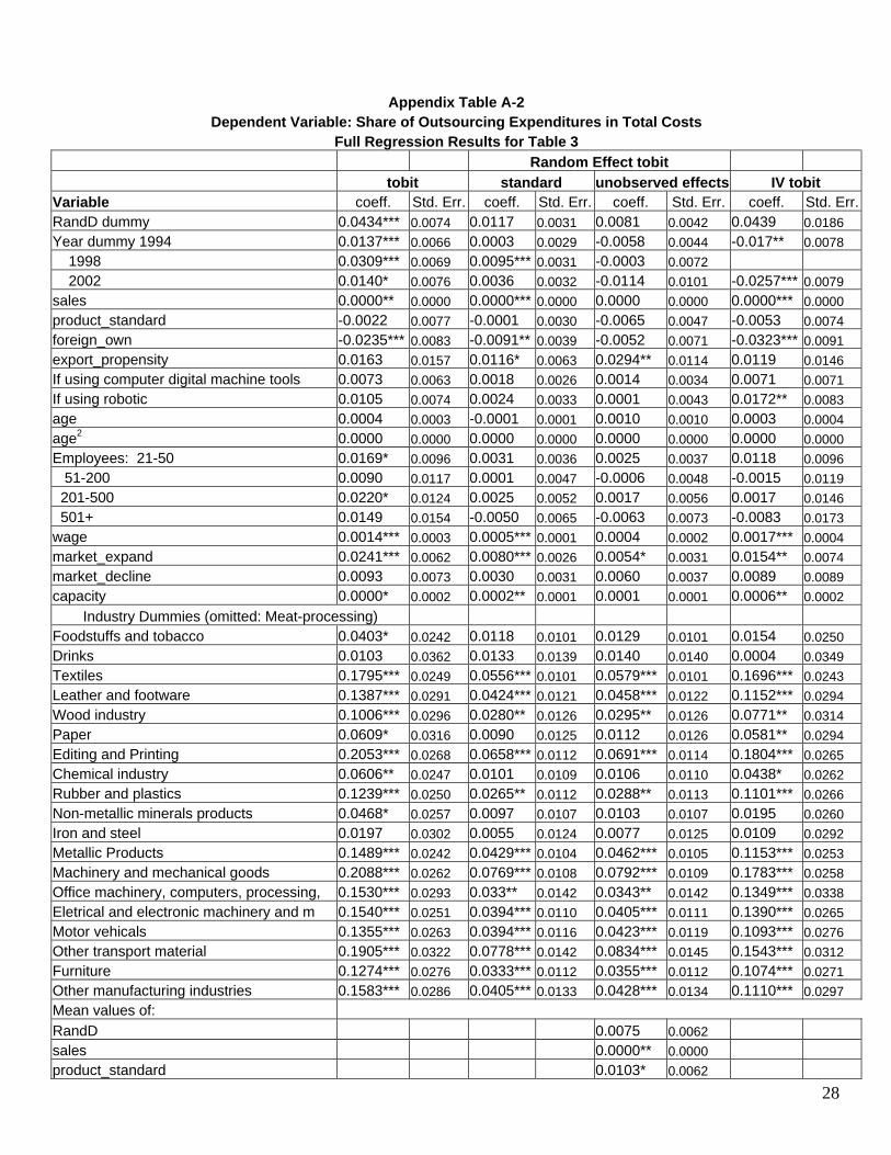
Appendix Table A-2

Dependent Variable: Share of Outsourcing Expenditures in Total Costs Full Regression Results for Table 3

Random Effect tobit tobit standard unobserved effects IV tobit Variable coeff. Std. Err. coeff. Std. Err. coeff. Std. Err. coeff. Std. Err.RandD dummy 0.0434*** 0.0074 0.0117 0.0031 0.0081 0.0042 0.0439 0.0186 Year dummy 1994 0.0137*** 0.0066 0.0003 0.0029 -0.0058 0.0044 -0.017** 0.0078 1998 0.0309*** 0.0069 0.0095*** 0.0031 -0.0003 0.0072 2002 0.0140* 0.0076 0.0036 0.0032 -0.0114 0.0101 -0.0257*** 0.0079 sales 0.0000** 0.0000 0.0000*** 0.0000 0.0000 0.0000 0.0000*** 0.0000 product_standard -0.0022 0.0077 -0.0001 0.0030 -0.0065 0.0047 -0.0053 0.0074 foreign_own -0.0235*** 0.0083 -0.0091** 0.0039 -0.0052 0.0071 -0.0323*** 0.0091 export_propensity 0.0163 0.0157 0.0116* 0.0063 0.0294** 0.0114 0.0119 0.0146 If using computer digital machine tools 0.0073 0.0063 0.0018 0.0026 0.0014 0.0034 0.0071 0.0071 If using robotic 0.0105 0.0074 0.0024 0.0033 0.0001 0.0043 0.0172** 0.0083 age 0.0004 0.0003 -0.0001 0.0001 0.0010 0.0010 0.0003 0.0004 age2 0.0000 0.0000 0.0000 0.0000 0.0000 0.0000 0.0000 0.0000 Employees: 21-50 0.0169* 0.0096 0.0031 0.0036 0.0025 0.0037 0.0118 0.0096 51-200 0.0090 0.0117 0.0001 0.0047 -0.0006 0.0048 -0.0015 0.0119 201-500 0.0220* 0.0124 0.0025 0.0052 0.0017 0.0056 0.0017 0.0146 501+ 0.0149 0.0154 -0.0050 0.0065 -0.0063 0.0073 -0.0083 0.0173 wage 0.0014*** 0.0003 0.0005*** 0.0001 0.0004 0.0002 0.0017*** 0.0004 market_expand 0.0241*** 0.0062 0.0080*** 0.0026 0.0054* 0.0031 0.0154** 0.0074 market_decline 0.0093 0.0073 0.0030 0.0031 0.0060 0.0037 0.0089 0.0089 capacity 0.0000* 0.0002 0.0002** 0.0001 0.0001 0.0001 0.0006** 0.0002

Industry Dummies (omitted: Meat-processing) Foodstuffs and tobacco 0.0403* 0.0242 0.0118 0.0101 0.0129 0.0101 0.0154 0.0250 Drinks 0.0103 0.0362 0.0133 0.0139 0.0140 0.0140 0.0004 0.0349 Textiles 0.1795*** 0.0249 0.0556*** 0.0101 0.0579*** 0.0101 0.1696*** 0.0243 Leather and footware 0.1387*** 0.0291 0.0424*** 0.0121 0.0458*** 0.0122 0.1152*** 0.0294 Wood industry 0.1006*** 0.0296 0.0280** 0.0126 0.0295** 0.0126 0.0771** 0.0314 Paper 0.0609* 0.0316 0.0090 0.0125 0.0112 0.0126 0.0581** 0.0294 Editing and Printing 0.2053*** 0.0268 0.0658*** 0.0112 0.0691*** 0.0114 0.1804*** 0.0265 Chemical industry 0.0606** 0.0247 0.0101 0.0109 0.0106 0.0110 0.0438* 0.0262 Rubber and plastics 0.1239*** 0.0250 0.0265** 0.0112 0.0288** 0.0113 0.1101*** 0.0266 Non-metallic minerals products 0.0468* 0.0257 0.0097 0.0107 0.0103 0.0107 0.0195 0.0260 Iron and steel 0.0197 0.0302 0.0055 0.0124 0.0077 0.0125 0.0109 0.0292 Metallic Products 0.1489*** 0.0242 0.0429*** 0.0104 0.0462*** 0.0105 0.1153*** 0.0253 Machinery and mechanical goods 0.2088*** 0.0262 0.0769*** 0.0108 0.0792*** 0.0109 0.1783*** 0.0258 Office machinery, computers, processing, 0.1530*** 0.0293 0.033** 0.0142 0.0343** 0.0142 0.1349*** 0.0338 Eletrical and electronic machinery and m 0.1540*** 0.0251 0.0394*** 0.0110 0.0405*** 0.0111 0.1390*** 0.0265 Motor vehicals 0.1355*** 0.0263 0.0394*** 0.0116 0.0423*** 0.0119 0.1093*** 0.0276 Other transport material 0.1905*** 0.0322 0.0778*** 0.0142 0.0834*** 0.0145 0.1543*** 0.0312 Furniture 0.1274*** 0.0276 0.0333*** 0.0112 0.0355*** 0.0112 0.1074*** 0.0271 Other manufacturing industries 0.1583*** 0.0286 0.0405*** 0.0133 0.0428*** 0.0134 0.1110*** 0.0297 Mean values of: RandD 0.0075 0.0062 sales 0.0000** 0.0000 product_standard 0.0103* 0.0062

29

foreign_own -0.0055 0.0086 export_propensity -0.0271** 0.0136 If using computer digital machine tools 0.0007 0.0054 If using robotic 0.0044 0.0067 age -0.0012 0.0010 age2 0.0000 0.0000 employment 0.0000 0.0000 wage 0.0001 0.0003 market_expand 0.0079 0.0056 market_decline -0.0078 0.0066 capacity 0.0002 0.0002 constant -0.3022*** 0.0312 -0.0242** 0.0121 -0.0292* 0.0157 -0.248*** 0.0320 * Significant at 10%. **Significant at 5%; ***Significant at 1%