Transportation Economic and Land Use System (TELUS)

Overview and Documentation of the TELUS

Economic Input-Output Model

M. H. Robison Economic Modeling Specialists, Inc. M. L. Lahr Rutgers University, Center for Urban Policy Research J. P. Berning Economic Modeling Specialists, Inc.

November, 2004

Table of Contents

1. Introduction ................................................................................................................................ 1

1.1. Challenges Posed by the TELUS IO Component ............................................................2

2. The TELUS Multiregional IO (MRIO) Algorithm ................................................................... 4

2.1. Mathematics of the Single Region Model.........................................................................4

2.2. The Rutgers RPC Estimating Equation ............................................................................4

2.3. Mathematics of the Multiregional Model.........................................................................7

2.4. Data Sources for Model Construction ..............................................................................8

3. Selecting Regions for MRIO Modeling.................................................................................... 12

3.1. Central Place Theory.........................................................................................................13

3.2. The Problem of Spillovers and Feedbacks......................................................................14

3.3. Spatial Misspecification Error..........................................................................................17

4. Resources for Identifying Central Place Hierarchies.............................................................. 20

4.1. BEA Economic Areas ........................................................................................................20

4.2. Rand McNally Trading Areas ..........................................................................................20

4.3. National Transportation Analysis Regions (NTARs)...................................................21

5. Distance Matrices...................................................................................................................... 23

5.1. Development of Distance Matrices .................................................................................23

6. MPO Maps................................................................................................................................. 25

6.1. MPO Regions .....................................................................................................................25

Appendices ...................................................................................................................................... 26

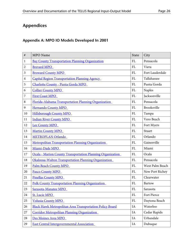
Appendix A: MPO IO Models Developed In 2001 .................................................................26

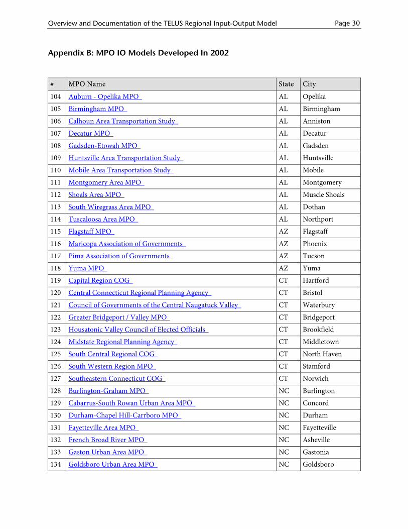
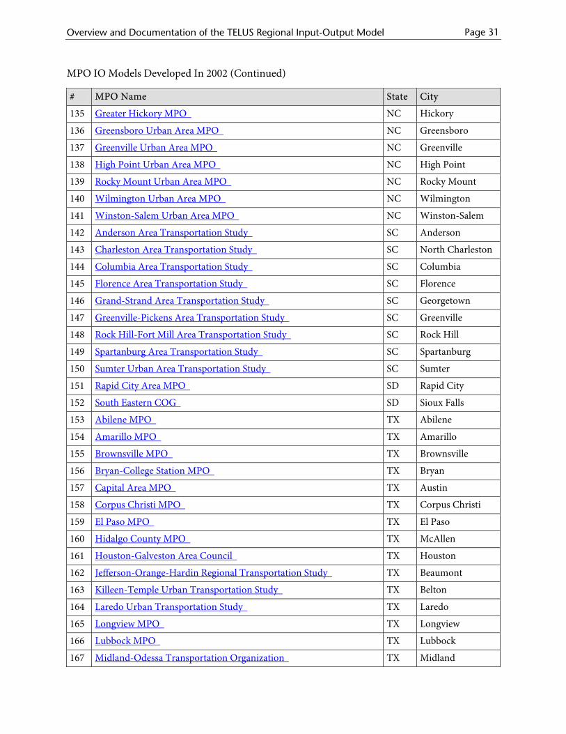
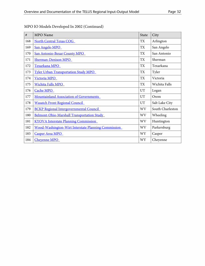
Appendix B: MPO IO Models Developed In 2002..................................................................30

Appendix C: MPO IO Models Developed In 2003 .................................................................33

Appendix D: MPO IO Models Developed In 2004.................................................................36

Appendix E: Phoenix MPO Distance Matrix ..........................................................................39

Appendix F: Map of Arkansas Meta-Region ...........................................................................40

Bibliography .................................................................................................................................... 41

Overview and Documentation of the TELUS Regional Input-Output Model Page 1

1. Introduction

The present document represents a thorough rewrite of the earlier TELUS IO model

(Transportation, Economic and Land-Use System, Input-Output) documenting report: A

Regional Input-Output Model for Estimating Economic Impacts in TELUS: Role, Data Sources and

Technical Specifications, (H. Robison and K. Gneiting, November 26, 1999). The earlier report

presented data sources and methods for building single-region models and the outlines of an

algorithm for estimating interregional trade as needed for the inter-county and rest-of-state

impacts aspect of the TELUS IO component. The paper was presented at the TELUS IO Model

Peer Review Meeting at NJIT (New Jersey Institute of Technology) in November 1999. During

the 2001 EMSI-NJIT contract year, EMSI (Economic Modeling Specialists, Inc.) built models

reflecting the earlier documentation for the 105 MPOs (Metropolitan Planning Organizations)

shown in Appendix A.

Starting with the 2002 EMSI-NJIT contract year, models were built utilizing the Rutgers

University, CUPR R/ECON I-O (Center for Urban Policy Research) modeling system. The

R/ECON system has been custom-outfitted with the interregional trade algorithm utilized by

EMSI in building models the first year, i.e., models constructed during the 2001 EMSI-NJIT

contract year for the MPOs shown in Appendix A. Given the basic similarity in data sources

between the EMSI and R/ECON models, the resulting TELUS models should be fundamentally

the same.1 The 82 models completed in 2002, 79 models in 2003, and 74 models in 2004 are

shown in Appendices B, C, and D respectively.

1 One difference between the first year EMSI models and R/ECON models pertains to aggregation. Given computer improvements since the 1999 design date of the original EMSI IO modeling software, the R/ECON software permits construction of individual region models with the full sectoral detail of the U.S. National IO model, approximately 500 sectors. In contrast, the original EMSI software required sectoral aggregation down to the approximately 50 sectors directly impacted by transportation projects. The original EMSI approach thereby results in a degree of aggregation error, though assuring that “first-order aggregation error” will be zero (see: Morimoto, 1970).

Overview and Documentation of the TELUS Regional Input-Output Model Page 2

A key component of the TELUS IO model is a set of translators that capture the direct spending

effect of transportation construction projects. The TELUS IO model requires 100 translators for

each state, or 5,000 translators overall. Documentation of the translator assembly process

appears in a separate EMSI documents: TRANSLATOR DOCUMENTATION: Mapping

Transportation Construction and Maintenance Projects into Economic Sectors for Use in the

TELUS Multiregional Input-Output Model, (H. Robison and W. Webb, December, 2002) and

EMSI Process for Translator Development.

1.1. Challenges Posed by the TELUS IO Component

Constructing an IO component for TELUS presents special challenges. Impacts are to be

estimated and displayed for each MPO County, and for the rest of the host state.2 MPOs may

consist of many counties. The Dallas-Fort Worth MPO, for example, has 16 counties, requiring a

model with 17 regions; the 17th region represents the rest of the state of Texas. As discussed

below, theoretical considerations require additional sub-regional delineation. With current

regional IO modeling technique calling for single-region base models with approximately 500

industrial sectors, the size of a full multiregional IO model might be 10,000 x 10,000 or more in

the case of a 20-region model (500 sectors x 20 regions). Addressing the size of a multiregional

model alone is therefore a challenge.

Building TELUS IO components poses other challenges as well. While the procedures for

building single-region models are well established,3 the same cannot be said of multi-region

models. Previous applications have employed a type of gravity mechanism (see for example

2 TELUS displays job, income, and gross regional product impacts for five industrial sectors, construction, manufacturing, retail/wholesale, services, and government/other. In addition, aggregate impacts are shown for state, local and federal taxes. The various impact measures are displayed for the individual counties of the MPO, the MPO as a whole (i.e., sum of county impacts), to the state economy outside the MPO, and for the state as a whole (i.e., sum of MPO plus in-state but out-of-MPO impacts). 3 Nowadays, best practice calls for some variation on the econometric approach first proposed by Stevens and others.

Overview and Documentation of the TELUS Regional Input-Output Model Page 3

Leontief and Strout, 1963 and Polenske, 1980), or they have assumed trade patterns based on

apparent hierarchical trade relationships (see for example Robison, 1984). The approach

adopted for the TELUS IO module combines elements of both applications by applying a gravity

component to the study regions defined on principles of hierarchical trade theory.

Overview and Documentation of the TELUS Regional Input-Output Model Page 4

2. The TELUS Multiregional IO (MRIO) Algorithm

2.1. Mathematics of the Single Region Model

Equation (1) shows the basic transformation of the national IO coefficients matrix into a regional

IO coefficients matrix for region r.

{ }ˆrr rrA Aγ= (1)

where:

Arr = regional coefficients matrix

A = national coefficients matrix

A single superscripted r would normally suffice to denote a single region r. The adoption of dual

superscripts anticipates multiregional formulations described below. The pre-multiplying array

γ̂ is a diagonal matrix of regional purchase coefficients (RPC). In general, these illustrate the

portion of regional demand satisfied by regional supplies.

2.2. The Rutgers RPC Estimating Equation

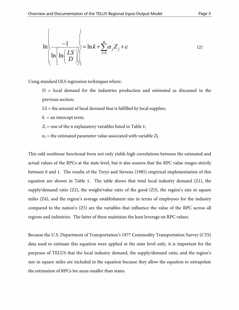
Adjustments for interregional trade4 are made using techniques developed by Treyz and Stevens

(1985, pp. 553-554). In this paper, the authors show that they estimate the regional purchase

coefficients (RPC) – the proportion of demand for an industry’s goods or services that is fulfilled

by local suppliers – using the following equation (2):

4 These adjustments do not account for international exports.

Overview and Documentation of the TELUS Regional Input-Output Model Page 5

1

1ln lnln ln

n

j ji

k ZLSD

α ε=

⎧ ⎫⎪ ⎪⎪ ⎪⎪ ⎪⎨ ⎬

⎡ ⎤⎛ ⎞⎪ ⎪⎢ ⎥⎜ ⎟⎪ ⎪⎜ ⎟⎢ ⎥⎪ ⎪⎝ ⎠⎣ ⎦⎩ ⎭

− = + +∑ (2)

Using standard OLS regression techniques where:

D = local demand for the industries production and estimated as discussed in the

previous section;

LS = the amount of local demand that is fulfilled by local supplies;

k = an intercept term;

Zj = one of the n explanatory variables listed in Table 1;

αj = the estimated parameter value associated with variable Zj.

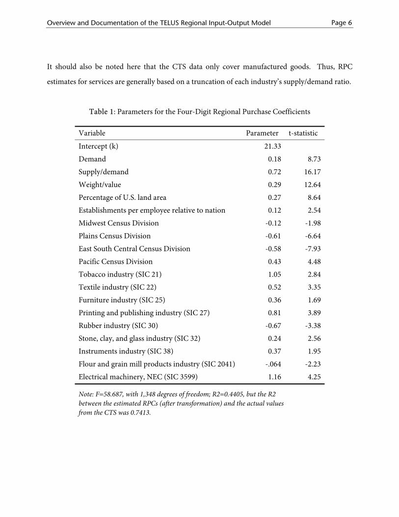
This odd nonlinear functional form not only yields high correlations between the estimated and

actual values of the RPCs at the state level, but it also assures that the RPC value ranges strictly

between 0 and 1. The results of the Treyz and Stevens (1985) empirical implementation of this

equation are shown in Table 1. The table shows that total local industry demand (Z1), the

supply/demand ratio (Z2), the weight/value ratio of the good (Z3), the region’s size in square

miles (Z4), and the region’s average establishment size in terms of employees for the industry

compared to the nation’s (Z5) are the variables that influence the value of the RPC across all

regions and industries. The latter of these maintains the least leverage on RPC values.

Because the U.S. Department of Transportation’s 1977 Commodity Transportation Survey (CTS)

data used to estimate this equation were applied at the state level only, it is important for the

purposes of TELUS that the local industry demand, the supply/demand ratio, and the region’s

size in square miles are included in the equation because they allow the equation to extrapolate

the estimation of RPCs for areas smaller than states.

Overview and Documentation of the TELUS Regional Input-Output Model Page 6

It should also be noted here that the CTS data only cover manufactured goods. Thus, RPC

estimates for services are generally based on a truncation of each industry’s supply/demand ratio.

Table 1: Parameters for the Four-Digit Regional Purchase Coefficients

Variable Parameter t-statistic

Intercept (k) 21.33

Demand 0.18 8.73

Supply/demand 0.72 16.17

Weight/value 0.29 12.64

Percentage of U.S. land area 0.27 8.64

Establishments per employee relative to nation 0.12 2.54

Midwest Census Division -0.12 -1.98

Plains Census Division -0.61 -6.64

East South Central Census Division -0.58 -7.93

Pacific Census Division 0.43 4.48

Tobacco industry (SIC 21) 1.05 2.84

Textile industry (SIC 22) 0.52 3.35

Furniture industry (SIC 25) 0.36 1.69

Printing and publishing industry (SIC 27) 0.81 3.89

Rubber industry (SIC 30) -0.67 -3.38

Stone, clay, and glass industry (SIC 32) 0.24 2.56

Instruments industry (SIC 38) 0.37 1.95

Flour and grain mill products industry (SIC 2041) -.064 -2.23

Electrical machinery, NEC (SIC 3599) 1.16 4.25

Note: F=58.687, with 1,348 degrees of freedom; R2=0.4405, but the R2 between the estimated RPCs (after transformation) and the actual values from the CTS was 0.7413.

Overview and Documentation of the TELUS Regional Input-Output Model Page 7

2.3. Mathematics of the Multiregional Model

The algorithm for estimating multiregional IO coefficients is illustrated with the example of an

economy with three sub-regions. The combined region is referred to as the meta-region. The

rational for identifying meta-regions and constituent sub-regions is discussed in sections below.

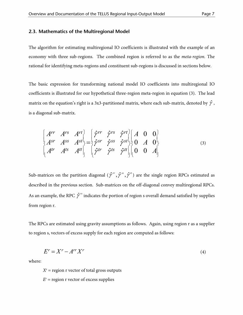
The basic expression for transforming national model IO coefficients into multiregional IO

coefficients is illustrated for our hypothetical three-region meta-region in equation (3). The lead

matrix on the equation’s right is a 3x3-partitioned matrix, where each sub-matrix, denoted by γ̂ ,

is a diagonal sub-matrix.

ˆ ˆ ˆ 0 0ˆ ˆ ˆ 0

0 0ˆ ˆ ˆ

rr rs rtrr rs rt

sr ss st sr ss st

tr ts tt tr ts tt

A A A AA A A A 0

AA A A

γ γ γγ γ γγ γ γ

⎧ ⎫⎧ ⎫ ⎧ ⎫⎪ ⎪⎪ ⎪ ⎪ ⎪

⎪ ⎪ ⎪ ⎪⎪⎨ ⎬ ⎨ ⎬⎨⎪ ⎪ ⎪ ⎪⎪⎪ ⎪ ⎪ ⎪⎪⎩ ⎭⎩ ⎭ ⎩ ⎭

= ⎪⎬⎪⎪

(3)

Sub-matrices on the partition diagonal ( ttssrr γγγ ˆ,ˆ,ˆ ) are the single region RPCs estimated as

described in the previous section. Sub-matrices on the off-diagonal convey multiregional RPCs.

As an example, the RPC rsγ̂ indicates the portion of region s overall demand satisfied by supplies

from region r.

The RPCs are estimated using gravity assumptions as follows. Again, using region r as a supplier

to region s, vectors of excess supply for each region are computed as follows:

r r rrE X A X= − r (4)

where:

Xr = region r vector of total gross outputs

Er = region r vector of excess supplies

Overview and Documentation of the TELUS Regional Input-Output Model Page 8

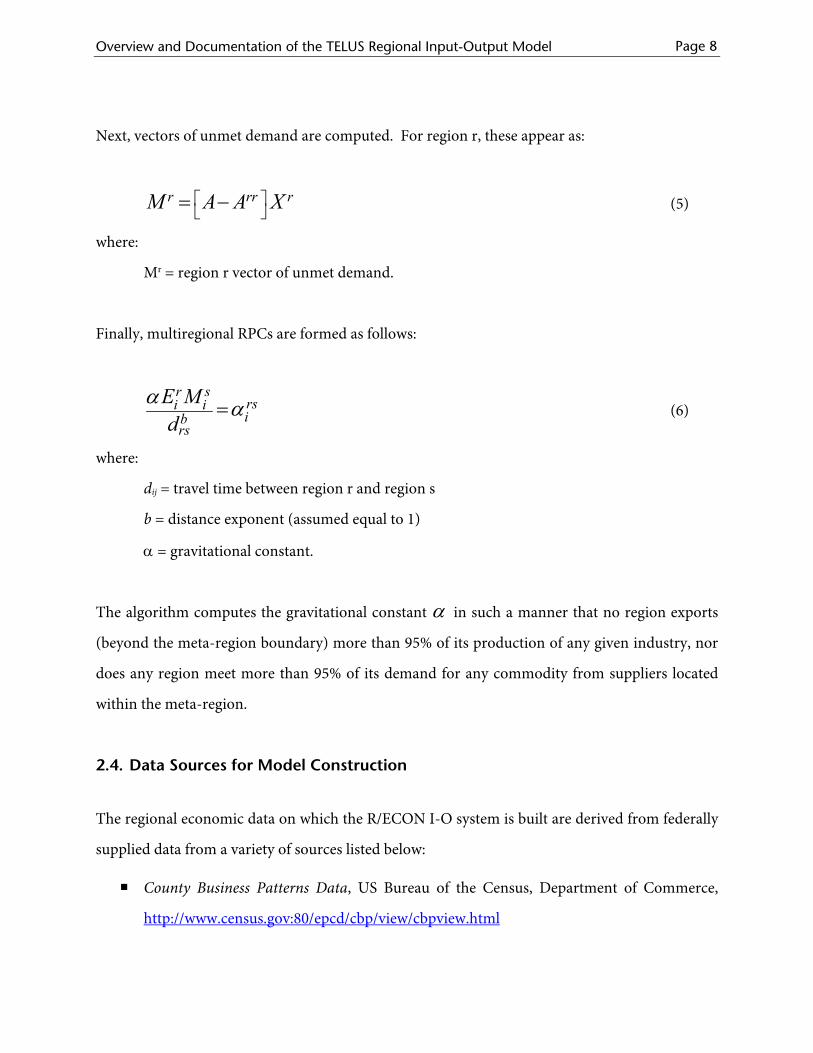
Next, vectors of unmet demand are computed. For region r, these appear as:

r rr rM A A X⎡ ⎤⎣ ⎦= − (5)

where:

Mr = region r vector of unmet demand.

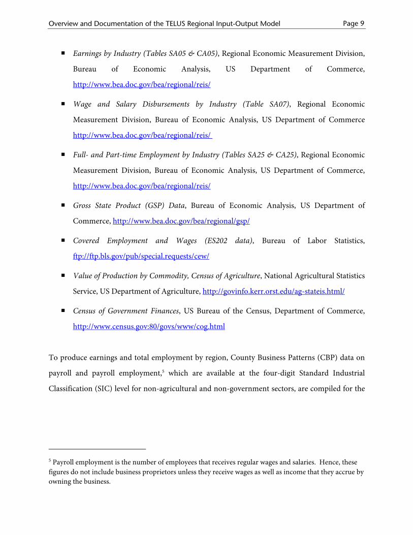
Finally, multiregional RPCs are formed as follows:

r srsi iib

rs

E Md

α α= (6)

where:

dij = travel time between region r and region s

b = distance exponent (assumed equal to 1)

α = gravitational constant.

The algorithm computes the gravitational constant α in such a manner that no region exports

(beyond the meta-region boundary) more than 95% of its production of any given industry, nor

does any region meet more than 95% of its demand for any commodity from suppliers located

within the meta-region.

2.4. Data Sources for Model Construction

The regional economic data on which the R/ECON I-O system is built are derived from federally

supplied data from a variety of sources listed below:

County Business Patterns Data, US Bureau of the Census, Department of Commerce,

http://www.census.gov:80/epcd/cbp/view/cbpview.html

Overview and Documentation of the TELUS Regional Input-Output Model Page 9

Earnings by Industry (Tables SA05 & CA05), Regional Economic Measurement Division,

Bureau of Economic Analysis, US Department of Commerce,

http://www.bea.doc.gov/bea/regional/reis/

Wage and Salary Disbursements by Industry (Table SA07), Regional Economic

Measurement Division, Bureau of Economic Analysis, US Department of Commerce

http://www.bea.doc.gov/bea/regional/reis/

Full- and Part-time Employment by Industry (Tables SA25 & CA25), Regional Economic

Measurement Division, Bureau of Economic Analysis, US Department of Commerce,

http://www.bea.doc.gov/bea/regional/reis/

Gross State Product (GSP) Data, Bureau of Economic Analysis, US Department of

Commerce, http://www.bea.doc.gov/bea/regional/gsp/

Covered Employment and Wages (ES202 data), Bureau of Labor Statistics,

ftp://ftp.bls.gov/pub/special.requests/cew/

Value of Production by Commodity, Census of Agriculture, National Agricultural Statistics

Service, US Department of Agriculture, http://govinfo.kerr.orst.edu/ag-stateis.html/

Census of Government Finances, US Bureau of the Census, Department of Commerce,

http://www.census.gov:80/govs/www/cog.html

To produce earnings and total employment by region, County Business Patterns (CBP) data on

payroll and payroll employment,5 which are available at the four-digit Standard Industrial

Classification (SIC) level for non-agricultural and non-government sectors, are compiled for the

5 Payroll employment is the number of employees that receives regular wages and salaries. Hence, these figures do not include business proprietors unless they receive wages as well as income that they accrue by owning the business.

Overview and Documentation of the TELUS Regional Input-Output Model Page 10

specified geography.6 The CBP payroll and payroll employment data are subsequently enhanced

using BEA’s state-level Table SA05 earnings/payroll and Table SA25 total-employment /payroll-

employment ratios at the two-digit SIC level. These ratios are then applied to the detailed sectors

in the economic model with which they are associated. Government enterprise and private

household employment are obtained separately from the ES202 files. Sub-national data on

agricultural income and employment by industry are derived using the region’s share of the

national value of production of the commodity. Thus, for agriculture only it is assumed that the

sector has the same average earnings per employee everywhere in the US.

To produce value-added and tax-revenue data, the value-added/earnings ratios by industry are

calculated from the two-digit SIC data and the data on earnings derived as discussed above.

Similar calculations from the same datasets are made to estimate indirect federal-government-

tax/earnings ratios and indirect state-and-local-government-tax/earnings ratios. The state-local

split of indirect business taxes and of personal taxes is calculated based on Census of Government

Finances data for the region. Wages net of taxes are estimated by calculating the share of

compensation from the GSP data files composed of the wages from BEA’s Table SA07, which are

also only available by state.

The estimated outputs by industry are derived from the labor-income coefficients of the

R/ECON I-O national I-O table and the earnings data discussed above. Lahr (2001) delves into a

more precise mathematical treatment of the techniques discussed here.

After the above data are collected, regional demand data by industry are estimated using the

techniques described in Treyz and Stevens (1985, equation 2). That is, in order to derive regional

demand by industry, the regional output estimates (obtained using the techniques discussed

6 The smaller a region is from an economic perspective, the greater are the number of the disclosure problems in CBP data. Hence, before using the CBP data in R/ECON I-O, all disclosure problems were filled in using a method like that described in Gerking et al. (2001).

Overview and Documentation of the TELUS Regional Input-Output Model Page 11

above) are first multiplied up the columns of the national direct-requirements matrix. The sums

of the rows of the resulting matrix are then obtained to get regional inter-industry demand. To

get total regional demand, of course, one must add to inter-industry demand the demand for

industry production placed by regional final demand i.e., locally based government operations,

regional households, and the region’s international exports. The product of regional output and

the national final-demand/output ratio estimates regional final demand by industry.

Overview and Documentation of the TELUS Regional Input-Output Model Page 12

3. Selecting Regions for MRIO Modeling

TELUS impact reporting requirements call for the estimation of impacts for each MPO County

and for the rest of the host state. Accordingly, single-region models must be constructed for

individual MPO counties, along with trade among these counties. But how should the rest-of-

state region, including trade between this region and the MPO counties be treated?

In general, rest-of-state areas will rarely appear as functioning economies appropriate for

treatment as stand-alone regions, but rather as doughnut areas with unconnected centers and

little internal cohesion. Correct treatment of rest-of-state areas will normally require that they be

viewed as composed of multiple, largely independent sub-regions. At a minimum then, trade

must be estimated among the rest-of-state sub-regions, and between these several sub-regions

and the counties of the MPO.

Unfortunately, the demands of the TELUS multiregional modeling problem do not stop here.

U.S. state and county boundaries are artifacts of 19th politics (Fox and Kumar, 1965). As a result,

economic boundaries routinely cross state lines, and this necessitates the inclusion of out-of-state

areas within the larger meta-region of the multiregional IO model. Omission of these out-of-

state areas, or failure to recognize the internal character of doughnut-shaped rest-of-state regions

results in predictable error in TELUS IO model impact estimates. This error is referred to as

spatial misspecification error. The next 4 sections present theory and guidelines to minimize

spatial misspecification error. The first section presents the outlines of central place theory, the

fundamental underpinning of regional definition. The second and third sections provide

alternative views of spatial misspecification error issue. The first considers the problem as one of

spillovers and feedbacks, while the second looks at it in a more technical sense. The final section

provides the practical resources used to identify economic sub-regions.

Overview and Documentation of the TELUS Regional Input-Output Model Page 13

3.1. Central Place Theory

Central place theory (Christaller, 1966 and Losch, 1954) provides the foundation for

characterizing the regional trade hierarchy. Central Place theory views the regional landscape

with sub-regions defined and ordered according to the goods and services they provide to

themselves and to other sub-regions (Berry et al., 1988). Parr (1987) provides taxonomy of goods

and services in a central place hierarchy, distinguishing between central place and specialized

goods and services. Central place goods and services include items for which there is essentially

ubiquitous demand: groceries, consumer durables, movies, air travel, accounting, legal and

business services, and so on. Specialized goods and services are items for which production is

unique to particular regions: agricultural products, timber, input-oriented manufacturing

military installations, federal government offices, and so on.

Lower-order sub-regions supply their own lower-order central place goods and services and

obtain higher-order central place goods and services from higher-order sub-regions. Higher-

order sub-regions supply their own lower-and higher-order central place goods and services.

There is no trade in central place goods and services between same-order sub-regions. Sub-

regions at the bottom of the trade hierarchy (lowest-order sub-regions) derive their income from

the export of specialized goods to other sub-regions for processing or outside the larger region.

Higher-order sub-regions derive their income from the supply of higher-order central place

goods and services to lower-order sub-regions and from the export of specialized goods to other

sub-regions and to outside the larger region.

TELUS reporting requirements call for the estimation of impacts that spill beyond MPO

boundaries to the rest of the state. This proves to be a complex endeavor. For one thing, the rest

of the state is almost never a functioning regional economy, and must therefore be subdivided

into multiple sub-regions. Beyond this, state boundaries are rarely economic boundaries, and

this requires the inclusion of out-of-state areas in the encompassing meta-region.

Overview and Documentation of the TELUS Regional Input-Output Model Page 14

3.2. The Problem of Spillovers and Feedbacks

The size and choice of sub-regions within the larger meta-region depends on the character of the

broader area trade hierarchy of which the state economy is a part. States differ not only in their

mix of industries, resource endowments and such, but also in their underlying spatial structures,

i.e., number, size, placement and interconnectedness of cities and towns. Regional IO models

capture the spread of multiplier effects among industries, and when space is included, as in the

multiregional model, they capture the spread of multiplier effects across places as well. Failure to

properly capture this spatial aspect of multiplier diffusion can lead to problems in spillover

estimation.

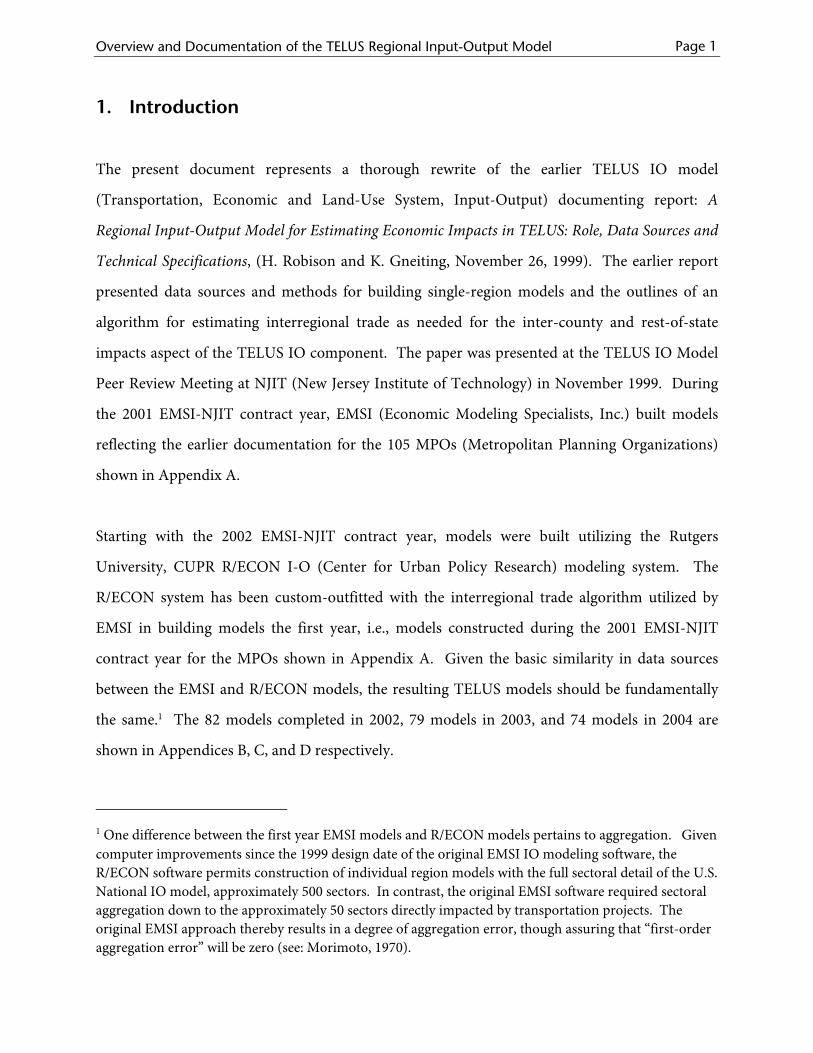
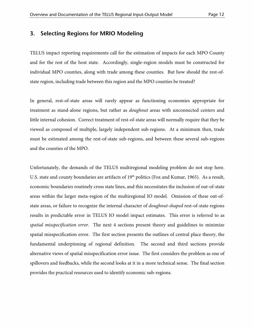
Consider a hypothetical example. Figure 1 shows an MPO surrounded by a trade-dominated

hinterland. Imagine a transportation project in the MPO that entails input purchases within the

MPO plus input purchases outside the MPO at location A. The project will create jobs and

incomes both in the MPO and in the vicinity of location A. However, by virtue of the MPOs

trade dominance of the hinterland including location A, we can expect feedback job and income

effects to the MPO. Failure to recognize the region’s spatial structure, specifically the MPOs

dominance of location A, could result in the omission of feedback effects, and the accompanying

understatement of MPO economic impacts.

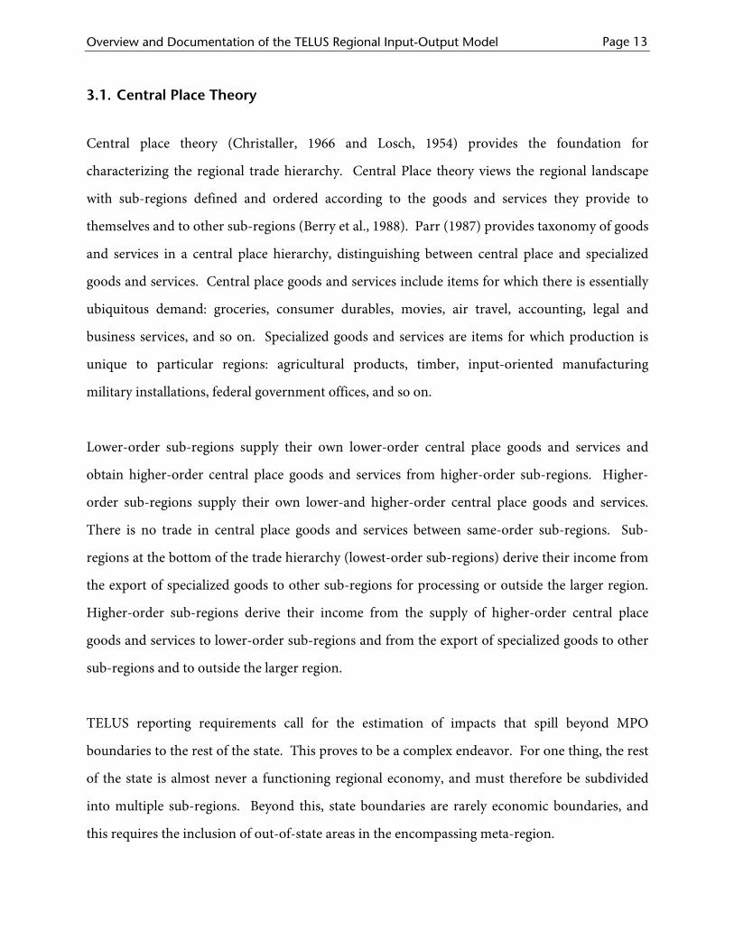
Figure 2 shows a variant on the case shown in Figure 1. This time the input supplier at location

A is in a neighboring state, and job and income effects in the vicinity of A are properly excluded

from the TELUS report. However, the feedback effect to the MPO is still in force, and failure to

recognize this would lead to an understatement of MPO impacts.

Overview and Documentation of the TELUS Regional Input-Output Model Page 15

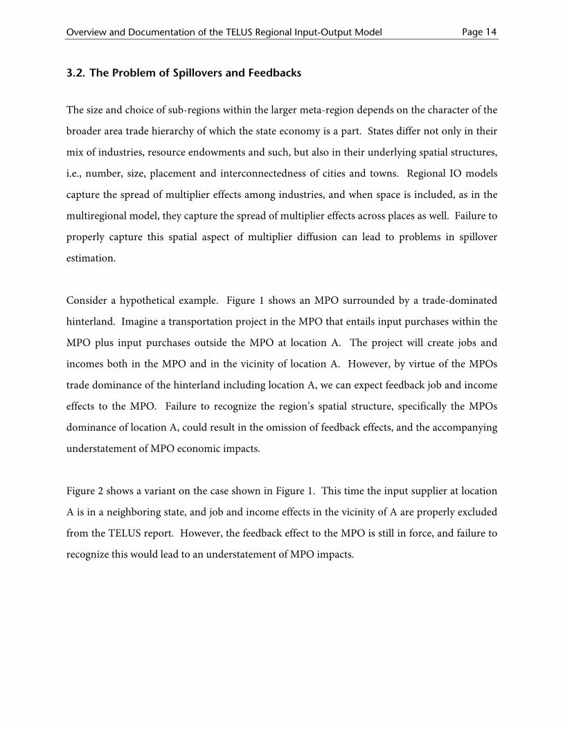
MPO A

Trade Area

Figure 1: An MPO and its trade partner (e.g. materials supplier B)

located within the same trade area

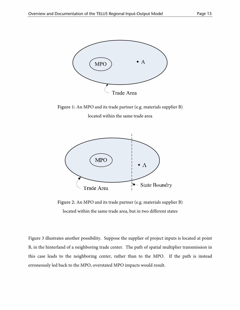
Figure 2: An MPO and its trade partner (e.g. materials supplier B)

located within the same trade area, but in two different states

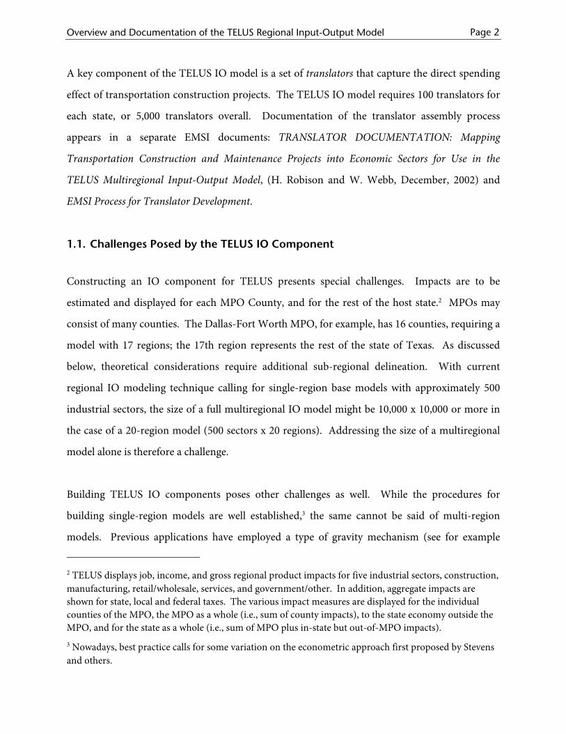
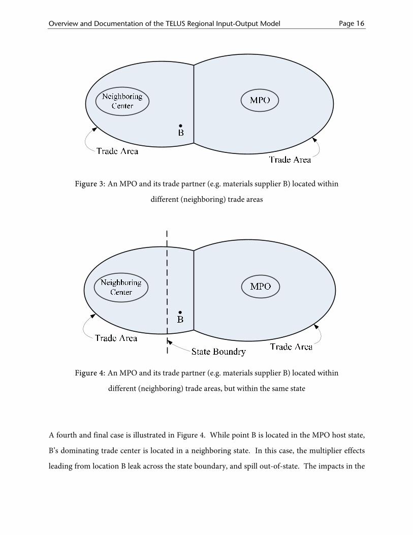
Figure 3 illustrates another possibility. Suppose the supplier of project inputs is located at point

B, in the hinterland of a neighboring trade center. The path of spatial multiplier transmission in

this case leads to the neighboring center, rather than to the MPO. If the path is instead

erroneously led back to the MPO, overstated MPO impacts would result.

Overview and Documentation of the TELUS Regional Input-Output Model Page 16

Figure 3: An MPO and its trade partner (e.g. materials supplier B) located within

different (neighboring) trade areas

Figure 4: An MPO and its trade partner (e.g. materials supplier B) located within

different (neighboring) trade areas, but within the same state

A fourth and final case is illustrated in Figure 4. While point B is located in the MPO host state,

B’s dominating trade center is located in a neighboring state. In this case, the multiplier effects

leading from location B leak across the state boundary, and spill out-of-state. The impacts in the

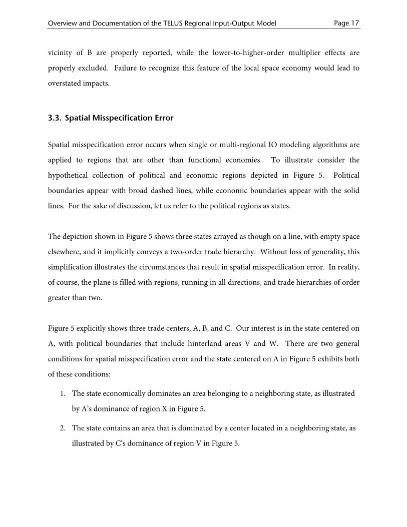
Overview and Documentation of the TELUS Regional Input-Output Model Page 17

vicinity of B are properly reported, while the lower-to-higher-order multiplier effects are

properly excluded. Failure to recognize this feature of the local space economy would lead to

overstated impacts.

3.3. Spatial Misspecification Error

Spatial misspecification error occurs when single or multi-regional IO modeling algorithms are

applied to regions that are other than functional economies. To illustrate consider the

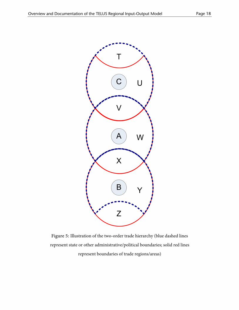
hypothetical collection of political and economic regions depicted in Figure 5. Political

boundaries appear with broad dashed lines, while economic boundaries appear with the solid

lines. For the sake of discussion, let us refer to the political regions as states.

The depiction shown in Figure 5 shows three states arrayed as though on a line, with empty space

elsewhere, and it implicitly conveys a two-order trade hierarchy. Without loss of generality, this

simplification illustrates the circumstances that result in spatial misspecification error. In reality,

of course, the plane is filled with regions, running in all directions, and trade hierarchies of order

greater than two.

Figure 5 explicitly shows three trade centers, A, B, and C. Our interest is in the state centered on

A, with political boundaries that include hinterland areas V and W. There are two general

conditions for spatial misspecification error and the state centered on A in Figure 5 exhibits both

of these conditions:

1. The state economically dominates an area belonging to a neighboring state, as illustrated

by A’s dominance of region X in Figure 5.

2. The state contains an area that is dominated by a center located in a neighboring state, as

illustrated by C’s dominance of region V in Figure 5.

Overview and Documentation of the TELUS Regional Input-Output Model Page 18

Figure 5: Illustration of the two-order trade hierarchy (blue dashed lines

represent state or other administrative/political boundaries; solid red lines

represent boundaries of trade regions/areas)

Overview and Documentation of the TELUS Regional Input-Output Model Page 19

The reason for the error is easily understood. The gravity method for estimating multiregional

trade operates on a supply-demand pooling mechanism. Surplus production in one region (i.e.,

production beyond local demand) is assumed available to meet otherwise unmet demand in

other regions, with near trade regions favored over distant trade regions. The solution of course

is to divide the larger area into component functional economies, and estimate the trade among

these smaller functional economic entities. This is the approach followed in constructing the

TELUS multiregional model.

Overview and Documentation of the TELUS Regional Input-Output Model Page 20

4. Resources for Identifying Central Place Hierarchies

4.1. BEA Economic Areas7

The U.S. Department of Commerce, Bureau of Economic Analysis divides the U.S. economy into

172 economic areas. Boundaries are drawn on economic rather than political or administrative

criteria. The work is clearly shaped by central place theory and the related notion of functional

economic areas (Fox and Kumar, 1965).

Each BEA economic area consists of a standard metropolitan statistical area (SMSA), or similar

area that serves as a center of trade, and the surrounding counties that are economically related

to the center. The delineation assures that each area will be relatively self-sufficient in the output

of its local service industries.

The 172 BEA economic areas are built-up from 348 smaller component economic areas (CEA).

CEAs are defined around a single economic node and the surrounding counties that are

economically related to the node. In a sense, therefore, a given BEA economic area can be

viewed as a three-order trade hierarchy, with the BEA core as the 3rd and highest order place,

followed by the centers of the CEAs (2nd order places), surrounded in turn by the dominated

CEA hinterlands.

4.2. Rand McNally Trading Areas

The Rand McNally Commercial Atlas and Marketing Guide (Rand McNally, 1999) provides an

alternative collection of central place-based trade areas. The elemental building blocks are 487

basic trading areas. These are areas surrounding at least one basic trading center. A basic trading

7 This description is excerpted from U.S. Department of Commerce, Bureau of Economic Analysis, 1975 and 1995.

Overview and Documentation of the TELUS Regional Input-Output Model Page 21

center is a city that serves as a center for the purchase of shopping goods. Basic trading areas

have apparel stores, general merchandise stores, and specialized services such as medical care,

entertainment, higher education and a daily newspaper. These follow county lines and are drawn

to include the county or counties whose residents make the bulk of their shopping goods

purchases in the area’s basic trading center(s) or its suburbs.

Moving up the trade hierarchy one level, the 487 basic trading areas are collected to into 47

major trading areas, each centered on its own major trading center. A major trading center is a

city that serves as one of the trading area’s primary centers for wholesaling, distribution, banking,

and specialized services such as advertising. The major trading area’s boundaries are determined

after “an intensive study” that considers such factors as physiography, population distributions,

newspaper circulation, economic activities, highway facilities, railroad services, suburban

transportation, and field reports of experienced sales analysts.

4.3. National Transportation Analysis Regions (NTARs)8

The U.S. Department of Transportation (DOT) has defined NTAR regions to “collect and

publish information on the interregional movements of goods, including the Commodity Flow

Survey (CFS).” NTAR boundaries, like those of the BEA economic areas and Rand McNally

trade areas, are constructed on principles grounded in central place theory. NTAR boundaries

recognize that transportation demand is molded by economic, social, and physical forces that

generally ignore political boundaries. Mountain ranges and the hinterlands of major economic

centers are just two of the many characteristics that affect patterns of transportation supply and

demand and have little correlation to state lines. NTAR regions are drawn according to

functional geography rather than by state or other political units.

8 This section is excerpted from the U.S. Department of Transportation, Bureau of Transportation Statistics website: http://www.bts.gov/programs/cfs/ntars/ntars.html

Overview and Documentation of the TELUS Regional Input-Output Model Page 22

NTARs are based on centers of population or economic activity that account for most of the

origins, destinations, or transfers of long-distance passenger and commodity movements. Each

region is defined to encompass the hinterland of the region's terminals for long distance

transportation. Where hinterlands of closely neighboring centers substantially overlap, the

regions are combined.

NTARs are defined as combinations of BEA economic areas, in part to be less numerous, and in

part to eliminate overlapping hinterlands. The result is 89 NTAR regions that reflect larger

centers and hinterlands than the 172 BEA economic areas, though in many cases smaller centers

and hinterlands than the 47 Rand McNally major trading areas.

Overview and Documentation of the TELUS Regional Input-Output Model Page 23

5. Distance Matrices

5.1. Development of Distance Matrices

To incorporate into the models the gravity mechanism that was previously mentioned, distance

matrices were built for each of the 85 MPO models. The distance matrices describe the average

time required to travel between each of the locations/regions used to build an MPO model. The

distance and the average travel time between locations/regions are used to determine the average

miles per hour. An adjustment is made to the miles per hour to calibrate for travel difficulty.

Unimpeded travel, as might be expected along an interstate highway, receives a degree of

difficulty of 1, which does not adjust the speed of travel. Moderately difficult travel receives a

degree of difficulty of 2 and the speed of travel is discounted by 20 percent. With travel that is

considered to be very difficult, such as in a highly congested city, the speed of travel is cut in half.

Then, an adjusted travel time is calculated using the distance and the adjusted miles per hour.

Travel within a location/region is estimated to be an average distance of 20 miles and is also

adjusted for a degree of difficulty. Travel to and from certain regions was estimated by selecting

a central location in the region as a reference point. For example, the region Jackson, AL (which

includes counties in Alabama that are affected by Jackson, MS) has Demopolis, AL as the

reference point for the distance matrix calculations.

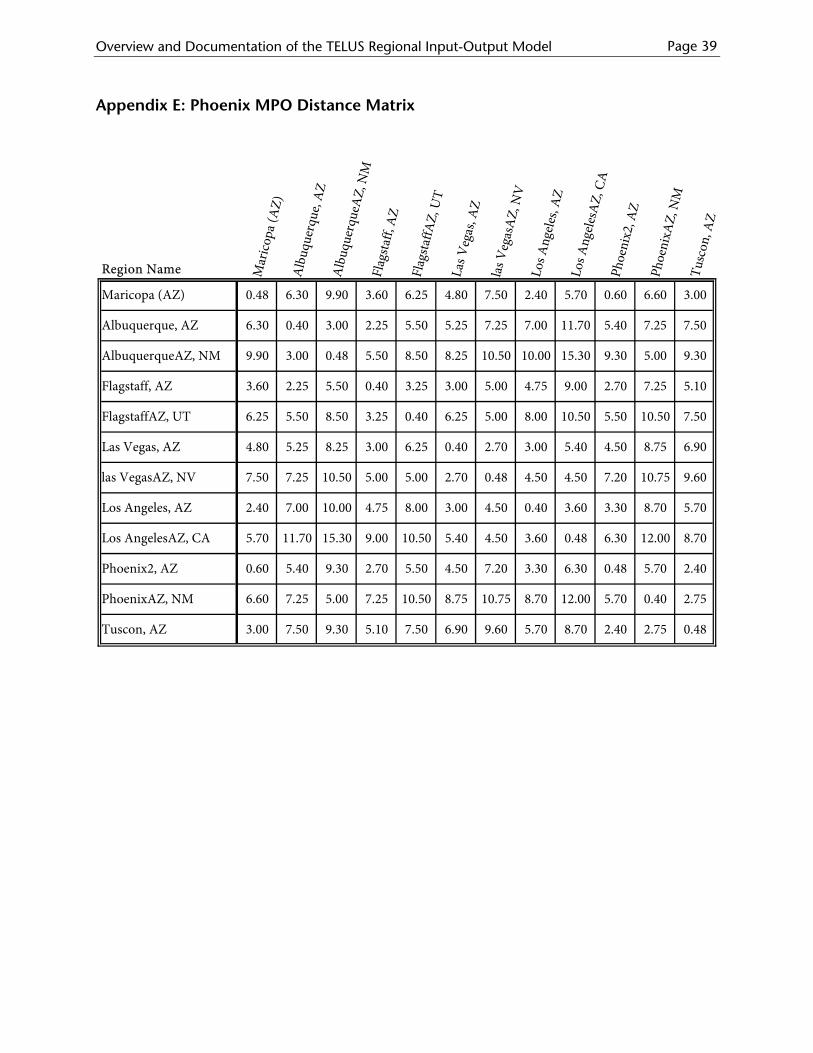
In order to discriminate between economic and political regions, as described in Section 3,

geographic regions were segmented to create the references used in the distance matrix. As an

example, Phoenix MPO has a distance matrix comprised of 12 cities/regions, including the single

MPO county Maricopa (shown in Appendix E), resulting in a 12 x 12. The matrix is built to

define the travel times between each pair of locations. To account for economic

interrelationships between different political (administrative) regions, the nearby Albuquerque

economic region was divided into two distinct segments: Albuquerque, New Mexico (denoted as

Overview and Documentation of the TELUS Regional Input-Output Model Page 24

AlbuquerqueAZ, NM) and Albuquerque, Arizona (denoted as Albuquerque, AZ). The former

represents the economic influence of the city of Albuquerque, NM on Phoenix, which is

contained within the political boundary of the State of New Mexico. The latter represents the

economic influence of the city of Albuquerque on Phoenix, which is contained within the

political boundary of the State of Arizona. The significance of this distinction was outlined in

Section 3.

These segmented regions were then used to estimate the gravity mechanism. As can be seen in

the Phoenix MPO distance matrix (Appendix E), adjusted travel time between AlbuquerqueAZ,

NM and Las VegasAZ, NV (which represents the economic influence of Las Vegas, NV on

Phoenix, which is contained in Nevada) is 10.5 hours. Adjusted travel time within Maricopa

County is 0.48 hours (20 miles of travel distance at an average of 50 mph, adjusted for a degree of

difficulty of 1.2).

Overview and Documentation of the TELUS Regional Input-Output Model Page 25

6. MPO Maps

6.1. MPO Regions

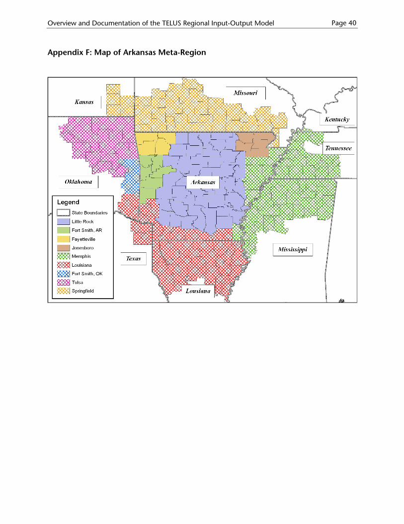
The maps of all states containing MPOs were created to highlight the economic and political

regions. An example of the Arkansas state map is shown in Appendix F. The outline of

Arkansas is represented by the thicker black lines, with portions of surrounding states being

included as necessary. The economic meta-region consists of sub-regions delineated by different

colors. The center of each sub-region is labeled accordingly. For example, the economic region

of Memphis, TN extends across Alabama, Arkansas, Kentucky, Louisiana, Missouri, and, of

course, Tennessee. This region is shown in Appendix F as the light blue cross-hatched region

labeled ‘Memphis’. This map describes the meta-region for all MPOs in Arkansas, and also aids

in designing the distance matrices described in the previous section.

Overview and Documentation of the TELUS Regional Input-Output Model Page 26

Appendices

Appendix A: MPO IO Models Developed In 2001

# MPO Name State City

1 Bay County Transportation Planning Organization FL Pensacola

2 Brevard MPO FL Viera

3 Broward County MPO FL Fort Lauderdale

4 Capital Region Transportation Planning Agency FL Tallahassee

5 Charlotte County - Punta Gorda MPO FL Punta Gorda

6 Collier County MPO FL Naples

7 First Coast MPO FL Jacksonville

8 Florida-Alabama Transportation Planning Organization FL Pensacola

9 Hernando County MPO FL Brooksville

10 Hillsborough County MPO FL Tampa

11 Indian River County MPO FL Vero Beach

12 Lee County MPO FL Fort Myers

13 Martin County MPO FL Stuart

14 METROPLAN Orlando FL Orlando

15 Metropolitan Transportation Planning Organization FL Gainesville

16 Miami-Dade MPO FL Miami

17 Ocala - Marion County Transportation Planning Organization FL Ocala

18 Okaloosa-Walton Transportation Planning Organization FL Pensacola

19 Palm Beach County MPO FL West Palm Beach

20 Pasco County MPO FL New Port Richey

21 Pinellas County MPO FL Clearwater

22 Polk County Transportation Planning Organization FL Bartow

23 Sarasota-Manatee MPO FL Sarasota

24 St. Lucie MPO FL Fort Pierce

25 Volusia County MPO FL Daytona Beach

26 Black Hawk Metropolitan Area Transportation Policy Board IA Waterloo

27 Corridor Metropolitan Planning Organization IA Cedar Rapids

28 Des Moines Area MPO IA Urbandale

29 East Central Intergovernmental Association IA Dubuque

Overview and Documentation of the TELUS Regional Input-Output Model Page 27

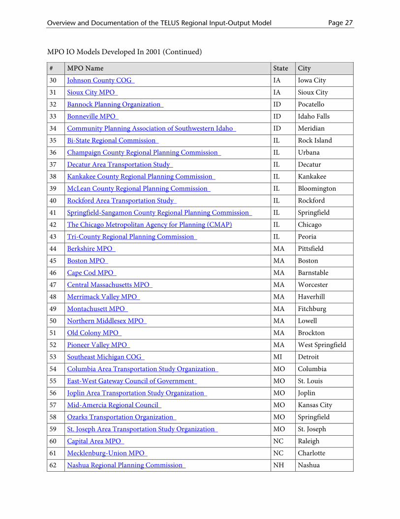
MPO IO Models Developed In 2001 (Continued)

# MPO Name State City

30 Johnson County COG IA Iowa City

31 Sioux City MPO IA Sioux City

32 Bannock Planning Organization ID Pocatello

33 Bonneville MPO ID Idaho Falls

34 Community Planning Association of Southwestern Idaho ID Meridian

35 Bi-State Regional Commission IL Rock Island

36 Champaign County Regional Planning Commission IL Urbana

37 Decatur Area Transportation Study IL Decatur

38 Kankakee County Regional Planning Commission IL Kankakee

39 McLean County Regional Planning Commission IL Bloomington

40 Rockford Area Transportation Study IL Rockford

41 Springfield-Sangamon County Regional Planning Commission IL Springfield

42 The Chicago Metropolitan Agency for Planning (CMAP) IL Chicago

43 Tri-County Regional Planning Commission IL Peoria

44 Berkshire MPO MA Pittsfield

45 Boston MPO MA Boston

46 Cape Cod MPO MA Barnstable

47 Central Massachusetts MPO MA Worcester

48 Merrimack Valley MPO MA Haverhill

49 Montachusett MPO MA Fitchburg

50 Northern Middlesex MPO MA Lowell

51 Old Colony MPO MA Brockton

52 Pioneer Valley MPO MA West Springfield

53 Southeast Michigan COG MI Detroit

54 Columbia Area Transportation Study Organization MO Columbia

55 East-West Gateway Council of Government MO St. Louis

56 Joplin Area Transportation Study Organization MO Joplin

57 Mid-Amercia Regional Council MO Kansas City

58 Ozarks Transportation Organization MO Springfield

59 St. Joseph Area Transportation Study Organization MO St. Joseph

60 Capital Area MPO NC Raleigh

61 Mecklenburg-Union MPO NC Charlotte

62 Nashua Regional Planning Commission NH Nashua

Overview and Documentation of the TELUS Regional Input-Output Model Page 28

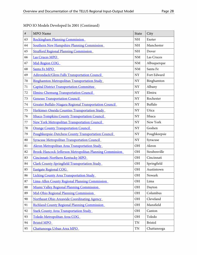
MPO IO Models Developed In 2001 (Continued)

# MPO Name State City

63 Rockingham Planning Commission NH Exeter

64 Southern New Hampshire Planning Commission NH Manchester

65 Strafford Regional Planning Commission NH Dover

66 Las Cruces MPO NM Las Cruces

67 Mid-Region COG NM Albuquerque

68 Santa Fe MPO NM Santa Fe

69 Adirondack/Glens Falls Transportation Council NY Fort Edward

70 Binghamton Metropolitan Transportation Study NY Binghamton

71 Capital District Transportation Committee NY Albany

72 Elmira-Chemung Transportation Council NY Elmira

73 Genesee Transportation Council NY Rochester

74 Greater Buffalo-Niagara Regional Transportation Council NY Buffalo

75 Herkimer-Oneida Counties Transportation Study NY Utica

76 Ithaca-Tompkins County Transportation Council NY Ithaca

77 New York Metropolitan Transportation Council NY New York

78 Orange County Transportation Council NY Goshen

79 Poughkeepsie-Dutchess County Transportation Council NY Poughkeepsie

80 Syracuse Metropolitan Transportation Council NY Syracuse

81 Akron Metropolitan Area Transportation Study OH Akron

82 Brook-Hancock-Jefferson Metropolitan Planning Commission OH Steubenville

83 Cincinnati-Northern Kentucky MPO OH Cincinnati

84 Clark County-Springfield Transportation Study OH Springfield

85 Eastgate Regional COG OH Austintown

86 Licking County Area Transportation Study OH Newark

87 Lima-Allen County Regional Planning Commission OH Lima

88 Miami Valley Regional Planning Commission OH Dayton

89 Mid-Ohio Regional Planning Commission OH Columbus

90 Northeast Ohio Areawide Coordinating Agency OH Cleveland

91 Richland County Regional Planning Commission OH Mansfield

92 Stark County Area Transportation Study OH Canton

93 Toledo Metropolitan Area COG OH Toledo

94 Bristol MPO TN Bristol

95 Chattanooga Urban Area MPO TN Chattanooga

Overview and Documentation of the TELUS Regional Input-Output Model Page 29

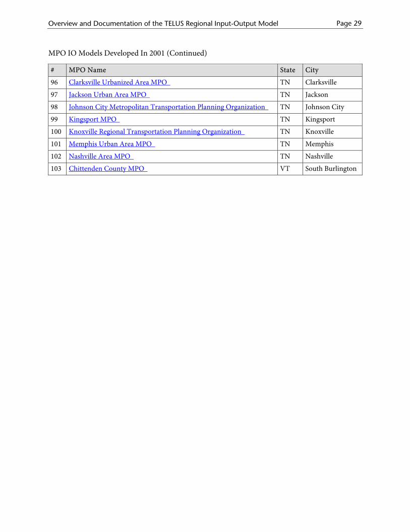
MPO IO Models Developed In 2001 (Continued)

# MPO Name State City

96 Clarksville Urbanized Area MPO TN Clarksville

97 Jackson Urban Area MPO TN Jackson

98 Johnson City Metropolitan Transportation Planning Organization TN Johnson City

99 Kingsport MPO TN Kingsport

100 Knoxville Regional Transportation Planning Organization TN Knoxville

101 Memphis Urban Area MPO TN Memphis

102 Nashville Area MPO TN Nashville

103 Chittenden County MPO VT South Burlington

Overview and Documentation of the TELUS Regional Input-Output Model Page 30

Appendix B: MPO IO Models Developed In 2002

# MPO Name State City

104 Auburn - Opelika MPO AL Opelika

105 Birmingham MPO AL Birmingham

106 Calhoun Area Transportation Study AL Anniston

107 Decatur MPO AL Decatur

108 Gadsden-Etowah MPO AL Gadsden

109 Huntsville Area Transportation Study AL Huntsville

110 Mobile Area Transportation Study AL Mobile

111 Montgomery Area MPO AL Montgomery

112 Shoals Area MPO AL Muscle Shoals

113 South Wiregrass Area MPO AL Dothan

114 Tuscaloosa Area MPO AL Northport

115 Flagstaff MPO AZ Flagstaff

116 Maricopa Association of Governments AZ Phoenix

117 Pima Association of Governments AZ Tucson

118 Yuma MPO AZ Yuma

119 Capital Region COG CT Hartford

120 Central Connecticut Regional Planning Agency CT Bristol

121 Council of Governments of the Central Naugatuck Valley CT Waterbury

122 Greater Bridgeport / Valley MPO CT Bridgeport

123 Housatonic Valley Council of Elected Officials CT Brookfield

124 Midstate Regional Planning Agency CT Middletown

125 South Central Regional COG CT North Haven

126 South Western Region MPO CT Stamford

127 Southeastern Connecticut COG CT Norwich

128 Burlington-Graham MPO NC Burlington

129 Cabarrus-South Rowan Urban Area MPO NC Concord

130 Durham-Chapel Hill-Carrboro MPO NC Durham

131 Fayetteville Area MPO NC Fayetteville

132 French Broad River MPO NC Asheville

133 Gaston Urban Area MPO NC Gastonia

134 Goldsboro Urban Area MPO NC Goldsboro

Overview and Documentation of the TELUS Regional Input-Output Model Page 31

MPO IO Models Developed In 2002 (Continued)

# MPO Name State City

135 Greater Hickory MPO NC Hickory

136 Greensboro Urban Area MPO NC Greensboro

137 Greenville Urban Area MPO NC Greenville

138 High Point Urban Area MPO NC High Point

139 Rocky Mount Urban Area MPO NC Rocky Mount

140 Wilmington Urban Area MPO NC Wilmington

141 Winston-Salem Urban Area MPO NC Winston-Salem

142 Anderson Area Transportation Study SC Anderson

143 Charleston Area Transportation Study SC North Charleston

144 Columbia Area Transportation Study SC Columbia

145 Florence Area Transportation Study SC Florence

146 Grand-Strand Area Transportation Study SC Georgetown

147 Greenville-Pickens Area Transportation Study SC Greenville

148 Rock Hill-Fort Mill Area Transportation Study SC Rock Hill

149 Spartanburg Area Transportation Study SC Spartanburg

150 Sumter Urban Area Transportation Study SC Sumter

151 Rapid City Area MPO SD Rapid City

152 South Eastern COG SD Sioux Falls

153 Abilene MPO TX Abilene

154 Amarillo MPO TX Amarillo

155 Brownsville MPO TX Brownsville

156 Bryan-College Station MPO TX Bryan

157 Capital Area MPO TX Austin

158 Corpus Christi MPO TX Corpus Christi

159 El Paso MPO TX El Paso

160 Hidalgo County MPO TX McAllen

161 Houston-Galveston Area Council TX Houston

162 Jefferson-Orange-Hardin Regional Transportation Study TX Beaumont

163 Killeen-Temple Urban Transportation Study TX Belton

164 Laredo Urban Transportation Study TX Laredo

165 Longview MPO TX Longview

166 Lubbock MPO TX Lubbock

167 Midland-Odessa Transportation Organization TX Midland

Overview and Documentation of the TELUS Regional Input-Output Model Page 32

MPO IO Models Developed In 2002 (Continued)

# MPO Name State City

168 North Central Texas COG TX Arlington

169 San Angelo MPO TX San Angelo

170 San Antonio-Bexar County MPO TX San Antonio

171 Sherman-Denison MPO TX Sherman

172 Texarkana MPO TX Texarkana

173 Tyler Urban Transportation Study MPO TX Tyler

174 Victoria MPO TX Victoria

175 Wichita Falls MPO TX Wichita Falls

176 Cache MPO UT Logan

177 Mountainland Association of Governments UT Orem

178 Wasatch Front Regional Council UT Salt Lake City

179 BCKP Regional Intergovernmental Council WV South Charleston

180 Belmont-Ohio-Marshall Transportation Study WV Wheeling

181 KYOVA Interstate Planning Commission WV Huntington

182 Wood-Washington-Wirt Interstate Planning Commission WV Parkersburg

183 Casper Area MPO WY Casper

184 Cheyenne MPO WY Cheyenne

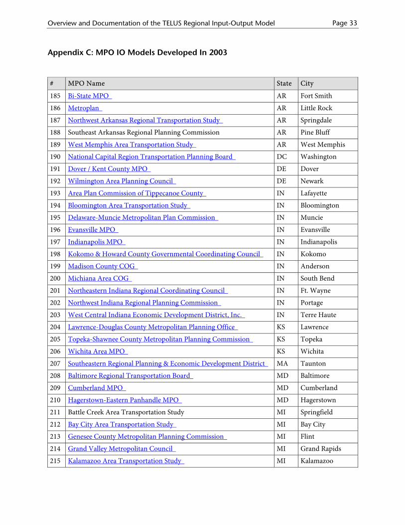
Overview and Documentation of the TELUS Regional Input-Output Model Page 33

Appendix C: MPO IO Models Developed In 2003

# MPO Name State City

185 Bi-State MPO AR Fort Smith

186 Metroplan AR Little Rock

187 Northwest Arkansas Regional Transportation Study AR Springdale

188 Southeast Arkansas Regional Planning Commission AR Pine Bluff

189 West Memphis Area Transportation Study AR West Memphis

190 National Capital Region Transportation Planning Board DC Washington

191 Dover / Kent County MPO DE Dover

192 Wilmington Area Planning Council DE Newark

193 Area Plan Commission of Tippecanoe County IN Lafayette

194 Bloomington Area Transportation Study IN Bloomington

195 Delaware-Muncie Metropolitan Plan Commission IN Muncie

196 Evansville MPO IN Evansville

197 Indianapolis MPO IN Indianapolis

198 Kokomo & Howard County Governmental Coordinating Council IN Kokomo

199 Madison County COG IN Anderson

200 Michiana Area COG IN South Bend

201 Northeastern Indiana Regional Coordinating Council IN Ft. Wayne

202 Northwest Indiana Regional Planning Commission IN Portage

203 West Central Indiana Economic Development District, Inc. IN Terre Haute

204 Lawrence-Douglas County Metropolitan Planning Office KS Lawrence

205 Topeka-Shawnee County Metropolitan Planning Commission KS Topeka

206 Wichita Area MPO KS Wichita

207 Southeastern Regional Planning & Economic Development District MA Taunton

208 Baltimore Regional Transportation Board MD Baltimore

209 Cumberland MPO MD Cumberland

210 Hagerstown-Eastern Panhandle MPO MD Hagerstown

211 Battle Creek Area Transportation Study MI Springfield

212 Bay City Area Transportation Study MI Bay City

213 Genesee County Metropolitan Planning Commission MI Flint

214 Grand Valley Metropolitan Council MI Grand Rapids

215 Kalamazoo Area Transportation Study MI Kalamazoo

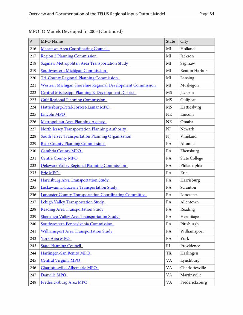
Overview and Documentation of the TELUS Regional Input-Output Model Page 34

MPO IO Models Developed In 2003 (Continued)

# MPO Name State City

216 Macatawa Area Coordinating Council MI Holland

217 Region 2 Planning Commission MI Jackson

218 Saginaw Metropolitan Area Transportation Study MI Saginaw

219 Southwestern Michigan Commission MI Benton Harbor

220 Tri-County Regional Planning Commission MI Lansing

221 Western Michigan Shoreline Regional Development Commission MI Muskegon

222 Central Mississippi Planning & Development District MS Jackson

223 Gulf Regional Planning Commission MS Gulfport

224 Hattiesburg-Petal-Forrest-Lamar MPO MS Hattiesburg

225 Lincoln MPO NE Lincoln

226 Metropolitan Area Planning Agency NE Omaha

227 North Jersey Transportation Planning Authority NJ Newark

228 South Jersey Transportation Planning Organization NJ Vineland

229 Blair County Planning Commission PA Altoona

230 Cambria County MPO PA Ebensburg

231 Centre County MPO PA State College

232 Delaware Valley Regional Planning Commission PA Philadelphia

233 Erie MPO PA Erie

234 Harrisburg Area Transportation Study PA Harrisburg

235 Lackawanna-Luzerne Transportation Study PA Scranton

236 Lancaster County Transportation Coordinating Committee PA Lancaster

237 Lehigh Valley Transportation Study PA Allentown

238 Reading Area Transportation Study PA Reading

239 Shenango Valley Area Transportation Study PA Hermitage

240 Southwestern Pennsylvania Commission PA Pittsburgh

241 Williamsport Area Transportation Study PA Williamsport

242 York Area MPO PA York

243 State Planning Council RI Providence

244 Harlingen-San Benito MPO TX Harlingen

245 Central Virginia MPO VA Lynchburg

246 Charlottesville-Albemarle MPO VA Charlottesville

247 Danville MPO VA Martinsville

248 Fredericksburg Area MPO VA Fredericksburg

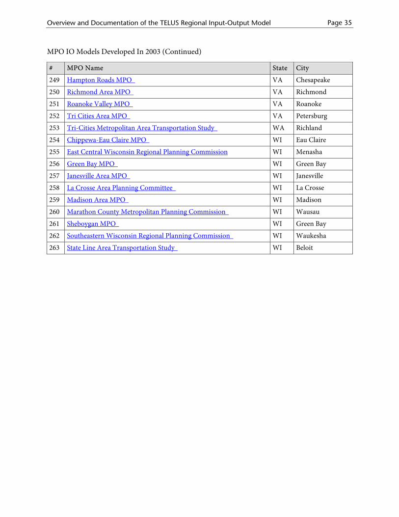
Overview and Documentation of the TELUS Regional Input-Output Model Page 35

MPO IO Models Developed In 2003 (Continued)

# MPO Name State City

249 Hampton Roads MPO VA Chesapeake

250 Richmond Area MPO VA Richmond

251 Roanoke Valley MPO VA Roanoke

252 Tri Cities Area MPO VA Petersburg

253 Tri-Cities Metropolitan Area Transportation Study WA Richland

254 Chippewa-Eau Claire MPO WI Eau Claire

255 East Central Wisconsin Regional Planning Commission WI Menasha

256 Green Bay MPO WI Green Bay

257 Janesville Area MPO WI Janesville

258 La Crosse Area Planning Committee WI La Crosse

259 Madison Area MPO WI Madison

260 Marathon County Metropolitan Planning Commission WI Wausau

261 Sheboygan MPO WI Green Bay

262 Southeastern Wisconsin Regional Planning Commission WI Waukesha

263 State Line Area Transportation Study WI Beloit

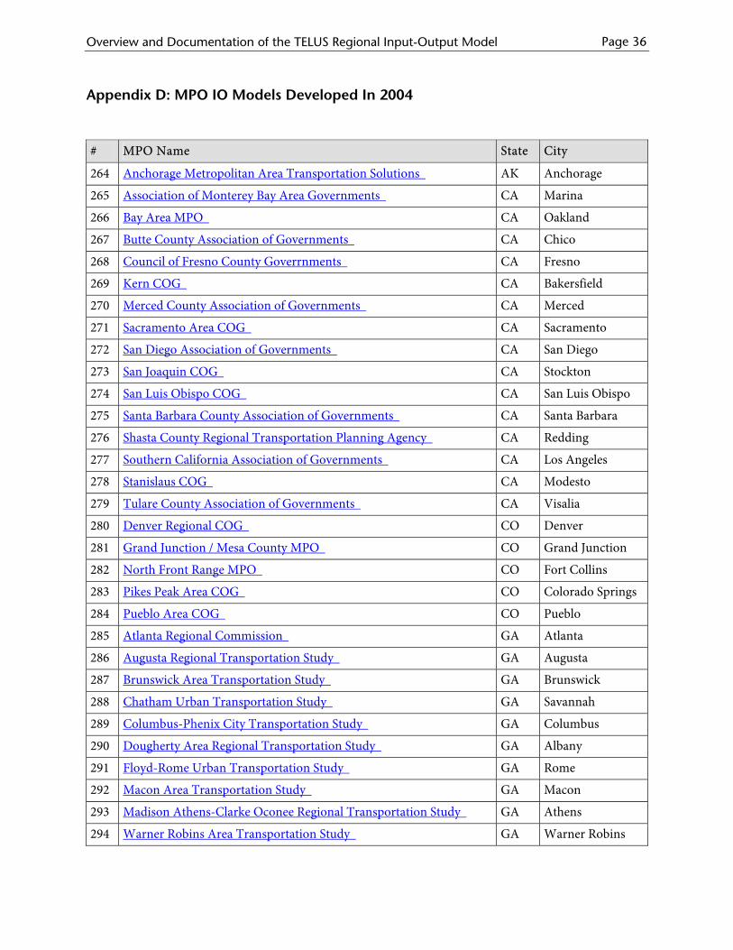
Overview and Documentation of the TELUS Regional Input-Output Model Page 36

Appendix D: MPO IO Models Developed In 2004

# MPO Name State City

264 Anchorage Metropolitan Area Transportation Solutions AK Anchorage

265 Association of Monterey Bay Area Governments CA Marina

266 Bay Area MPO CA Oakland

267 Butte County Association of Governments CA Chico

268 Council of Fresno County Goverrnments CA Fresno

269 Kern COG CA Bakersfield

270 Merced County Association of Governments CA Merced

271 Sacramento Area COG CA Sacramento

272 San Diego Association of Governments CA San Diego

273 San Joaquin COG CA Stockton

274 San Luis Obispo COG CA San Luis Obispo

275 Santa Barbara County Association of Governments CA Santa Barbara

276 Shasta County Regional Transportation Planning Agency CA Redding

277 Southern California Association of Governments CA Los Angeles

278 Stanislaus COG CA Modesto

279 Tulare County Association of Governments CA Visalia

280 Denver Regional COG CO Denver

281 Grand Junction / Mesa County MPO CO Grand Junction

282 North Front Range MPO CO Fort Collins

283 Pikes Peak Area COG CO Colorado Springs

284 Pueblo Area COG CO Pueblo

285 Atlanta Regional Commission GA Atlanta

286 Augusta Regional Transportation Study GA Augusta

287 Brunswick Area Transportation Study GA Brunswick

288 Chatham Urban Transportation Study GA Savannah

289 Columbus-Phenix City Transportation Study GA Columbus

290 Dougherty Area Regional Transportation Study GA Albany

291 Floyd-Rome Urban Transportation Study GA Rome

292 Macon Area Transportation Study GA Macon

293 Madison Athens-Clarke Oconee Regional Transportation Study GA Athens

294 Warner Robins Area Transportation Study GA Warner Robins

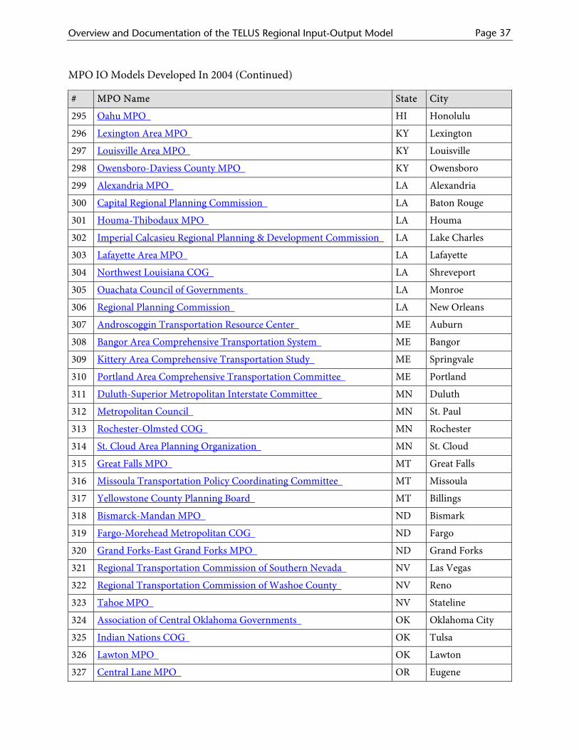
Overview and Documentation of the TELUS Regional Input-Output Model Page 37

MPO IO Models Developed In 2004 (Continued)

# MPO Name State City

295 Oahu MPO HI Honolulu

296 Lexington Area MPO KY Lexington

297 Louisville Area MPO KY Louisville

298 Owensboro-Daviess County MPO KY Owensboro

299 Alexandria MPO LA Alexandria

300 Capital Regional Planning Commission LA Baton Rouge

301 Houma-Thibodaux MPO LA Houma

302 Imperial Calcasieu Regional Planning & Development Commission LA Lake Charles

303 Lafayette Area MPO LA Lafayette

304 Northwest Louisiana COG LA Shreveport

305 Ouachata Council of Governments LA Monroe

306 Regional Planning Commission LA New Orleans

307 Androscoggin Transportation Resource Center ME Auburn

308 Bangor Area Comprehensive Transportation System ME Bangor

309 Kittery Area Comprehensive Transportation Study ME Springvale

310 Portland Area Comprehensive Transportation Committee ME Portland

311 Duluth-Superior Metropolitan Interstate Committee MN Duluth

312 Metropolitan Council MN St. Paul

313 Rochester-Olmsted COG MN Rochester

314 St. Cloud Area Planning Organization MN St. Cloud

315 Great Falls MPO MT Great Falls

316 Missoula Transportation Policy Coordinating Committee MT Missoula

317 Yellowstone County Planning Board MT Billings

318 Bismarck-Mandan MPO ND Bismark

319 Fargo-Morehead Metropolitan COG ND Fargo

320 Grand Forks-East Grand Forks MPO ND Grand Forks

321 Regional Transportation Commission of Southern Nevada NV Las Vegas

322 Regional Transportation Commission of Washoe County NV Reno

323 Tahoe MPO NV Stateline

324 Association of Central Oklahoma Governments OK Oklahoma City

325 Indian Nations COG OK Tulsa

326 Lawton MPO OK Lawton

327 Central Lane MPO OR Eugene

Overview and Documentation of the TELUS Regional Input-Output Model Page 38

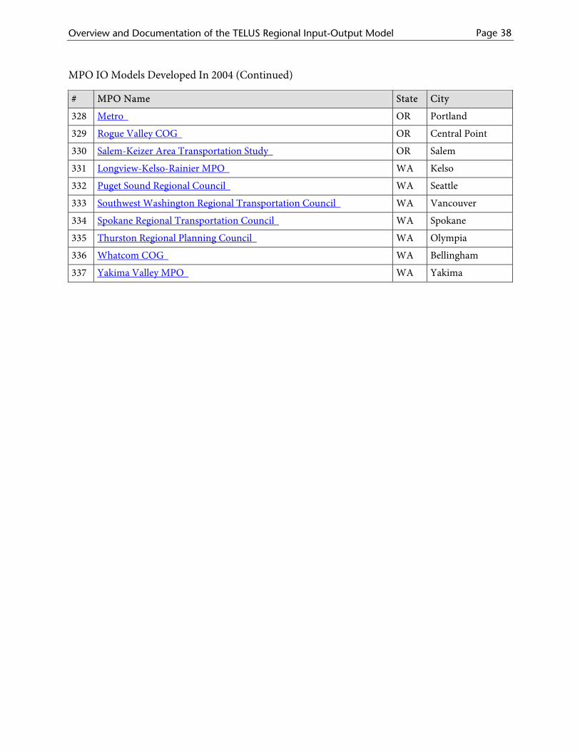
MPO IO Models Developed In 2004 (Continued)

# MPO Name State City

328 Metro OR Portland

329 Rogue Valley COG OR Central Point

330 Salem-Keizer Area Transportation Study OR Salem

331 Longview-Kelso-Rainier MPO WA Kelso

332 Puget Sound Regional Council WA Seattle

333 Southwest Washington Regional Transportation Council WA Vancouver

334 Spokane Regional Transportation Council WA Spokane

335 Thurston Regional Planning Council WA Olympia

336 Whatcom COG WA Bellingham

337 Yakima Valley MPO WA Yakima

Overview and Documentation of the TELUS Regional Input-Output Model Page 39

Appendix E: Phoenix MPO Distance Matrix

Region Name Mar

icop

a (A

Z)A

lbuq

uerq

ue, A

ZA

lbuq

uerq

ueA

Z, N

MFl

agst

aff,

AZ

Flag

staf

fAZ,

UT

Las V

egas

, AZ

las V

egas

AZ,

NV

Los A

ngel

es, A

ZLo

s Ang

eles

AZ,

CA

Phoe

nix2

, AZ

Phoe

nixA

Z, N

MTu

scon

, AZ

Maricopa (AZ) 0.48 6.30 9.90 3.60 6.25 4.80 7.50 2.40 5.70 0.60 6.60 3.00

Albuquerque, AZ 6.30 0.40 3.00 2.25 5.50 5.25 7.25 7.00 11.70 5.40 7.25 7.50

AlbuquerqueAZ, NM 9.90 3.00 0.48 5.50 8.50 8.25 10.50 10.00 15.30 9.30 5.00 9.30

Flagstaff, AZ 3.60 2.25 5.50 0.40 3.25 3.00 5.00 4.75 9.00 2.70 7.25 5.10

FlagstaffAZ, UT 6.25 5.50 8.50 3.25 0.40 6.25 5.00 8.00 10.50 5.50 10.50 7.50

Las Vegas, AZ 4.80 5.25 8.25 3.00 6.25 0.40 2.70 3.00 5.40 4.50 8.75 6.90

las VegasAZ, NV 7.50 7.25 10.50 5.00 5.00 2.70 0.48 4.50 4.50 7.20 10.75 9.60

Los Angeles, AZ 2.40 7.00 10.00 4.75 8.00 3.00 4.50 0.40 3.60 3.30 8.70 5.70

Los AngelesAZ, CA 5.70 11.70 15.30 9.00 10.50 5.40 4.50 3.60 0.48 6.30 12.00 8.70

Phoenix2, AZ 0.60 5.40 9.30 2.70 5.50 4.50 7.20 3.30 6.30 0.48 5.70 2.40

PhoenixAZ, NM 6.60 7.25 5.00 7.25 10.50 8.75 10.75 8.70 12.00 5.70 0.40 2.75

Tuscon, AZ 3.00 7.50 9.30 5.10 7.50 6.90 9.60 5.70 8.70 2.40 2.75 0.48

Overview and Documentation of the TELUS Regional Input-Output Model Page 40

Appendix F: Map of Arkansas Meta-Region

Overview and Documentation of the TELUS Regional Input-Output Model Page 41

Bibliography

Berry, B. J. L., J. B. Parr, B. J. Epstein, A. Ghosh, and R. H. T. Smith, 1988. Market Centers and

Retail Location, Theory and Applications. (Englewood Cliffs, Prentice Hall).

Christaller, W., 1966. Central Places in Southern Germany (C.W. Baskins, trans.). Englewood

Cliffs, NJ, Prentice Hall.

Fox, K. A. and K. Kumar. 1965. "The Functional Economic Area: Delineation and Implications

for Economic Analysis and Policy," Papers of Regional Science Association, 15, 57-85.

Gerkins, S. D., A.Isserman, W. Hamilton, T. Pickton, O.Smirnov, and D. Sorenson, 2001. “Anti-

suppressants and the creation and use of nonsurvey regional input-output models”. M.L. Lahr

and R. E. Miller, (ed.). Regional science perspectives in economic analysis: A festschrift in memory

of Benjamin H. Stevens. 379-306, Amsterdam: Elsevier Science.

Leontief, W. W. and A. Strout, 1963. "Multiregional Input-Output Analysis”, p.129-161, in

Input-Output Economics, 2nd Ed. Oxford University Press.

Losch, A., 1954. The Economics of Location (W. H. Woglom and W. F. Stolper, trans.). New

Haven: Yale University Press.

Morimoto, Y., 1970.”On Aggregation Problems in Input-Output Analysis”, Review of Economic

Studies, 119-126.

Parr, J. B., 1987. "Interaction in an Urban System: Aspects of Trade and Commuting," Economic

Geography, 63(3), 223-240.

Overview and Documentation of the TELUS Regional Input-Output Model Page 42

Polenske, K. R., 1980. The United States Multiregional Input-Output Accounts and Model,

(Lexington, MA, D.C. Heath).

Robison, M. H., J. R. Hamilton, K. P. Connaughton, N. Meyer and R. Coupal. 1994. "Spatial

Diffusion of Economic Impacts and Development Benefits in Hierarchically Structured Trade

Regions: An Empirical Application of Central Place-Based Input-Output Analysis," Review of

Regional Studies, 23(3), 307-326.

Treyz, G. and B. Stevens, 1985. “The TFS Regional Modeling Methodology,” Regional Studies,

19: 547-562.