Overview of the 2015 St. Patrick’s day storm and its consequencesfor RTK and PPP positioning in Norway

Knut Stanley Jacobsen* and Yngvild Linnea Andalsvik

Norwegian Mapping Authority, PO 600 Sentrum, 3507 Hønefoss, Norway*e-mail: knut.stanley.jacobsen@kartverket.no

Received 28 September 2015 / Accepted 21 January 2016

ABSTRACT

The 2015 St. Patrick’s day storm was the first storm of solar cycle 24 to reach a level of ‘‘Severe’’ on the NOAA geomagneticstorm scale. The Norwegian Mapping Authority is operating a national real-time kinematic (RTK) positioning network and has inrecent years developed software and services and deployed instrumentation to monitor space weather disturbances. Here, we re-port on our observations during this event. Strong GNSS (Global Navigation Satellite System) disturbances, measured by the rate-of-TEC index (ROTI), were observed at all latitudes in Norway on March 17th and early on March 18th. Late on the 18th, strongdisturbances were only observed in northern parts of Norway. We study the ionospheric disturbances in relation to the auroralelectrojet currents, showing that the most intense disturbances of GNSS signals occur on the poleward side of poleward-movingcurrent regions. This indicates a possible connection to ionospheric polar cap plasma patches and/or particle precipitation causedby magnetic reconnection in the magnetosphere tail. We also study the impact of the disturbances on the network RTK andPrecise Point Positioning (PPP) techniques. The vertical position errors increase rapidly with increasing ROTI for bothtechniques, but PPP is more precise than RTK at all disturbance levels.

Key words. Positioning system – Space weather – Storm – Ionosphere (auroral) – Irregularities

1. Introduction

On 17–18 March 2015, the first storm of solar cycle 24 to reachthe G4 level on the NOAA scale (Poppe 2000) occurred. AsMarch 17th is St. Patrick’s day, we will refer to the storm asthe St. Patrick’s day storm. The storm was notable for two rea-sons: the first that it was at that point the strongest storm of thesolar cycle, the second that space weather agencies around theworld failed to predict it. Geomagnetic storm warnings had beenissued, but only for a minor storm, which would not be a con-cern to most users. As an example, this is an extract of theweekly report by the space weather prediction centre of NOAA.1

Space weather outlook 16 March–11 April, 2015

Solar activity is expected to continue at moderate levelsuntil 19 March when Region 2297 transits off the visibledisk. � � �hsnipi� � � Geomagnetic field activity is expectedto be at unsettled to active levels with minor storm peri-ods likely on 18 March due to a combination of CH HSSeffects as well as the arrival of the 15 March CME bymid to late on 17 March.

The Norwegian Mapping Authority (NMA) is operating anational real-time kinematic (RTK) positioning network andhas in recent years developed software and services anddeployed instrumentation to monitor space weather distur-bances. We have previously reported on the impact of a strong(G3 level) and a less-than-minor (below the G-scale) geomag-netic storm on our RTK service (Jacobsen & Schäfer 2012;

Andalsvik & Jacobsen 2014). Since then, we have deployednew instrumentation and further developed our analysis capa-bility. In this paper we give an overview of the St. Patrick’sday storm event as observed from Norway, and its impact onpositioning using the network RTK and Precise Point Position-ing (PPP) techniques.

Network real-time kinematic (RTK) positioning is a process-ing technique in which a single user receiver receives supportingdata about several types of GNSS error sources from a networkof receivers (Frodge et al. 1994; Rizos 2003). This allows theuser receiver to eliminate a large part of the errors in the signaland thus achieve an accurate position solution in real-time. Atthe time of the event, the software used for the central networkprocessing at NMA was RTKNet, from the company Trimble.

Precise Point Positioning (PPP) is a single receiver process-ing strategy for GNSS observations that enables the efficientcomputation of high-quality coordinates, utilizing undiffer-enced dual-frequency code and phase observations by usingprecise satellite orbit and clock data products. More detaileddescriptions of PPP can be found in e.g. Zumberge et al.(1997) and Kouba & Héroux (2001).

Kamide & Kusano (2015) were the first to report on the StPatrick’s day storm in a scientific journal, in the form of a newsarticle in the Space Weather journal. In addition to a generaloverview and comments regarding the event, they suggestedthat it was caused by a superposition of two moderate events.Cherniak et al. (2015) studied the disturbances on a globalscale using data from more than 2500 GPS receivers. Theirpaper provides an excellent overview of the large-scale distri-bution and development of GPS disturbances.

One of the possible causes of GPS disturbances at high lat-itudes are polar cap patches, which are convecting clouds of

1 NOAA/SWPC, 2015, ftp://ftp.swpc.noaa.gov/pub/warehouse/2015/WeeklyPDF/prf2063.pdf

J. Space Weather Space Clim., 6, A9 (2016)DOI: 10.1051/swsc/2016004� K.S. Jacobsen and Y.L. Andalsvik, Published by EDP Sciences 2016

OPEN ACCESSRESEARCH ARTICLE

This is an Open Access article distributed under the terms of the Creative Commons Attribution License (http://creativecommons.org/licenses/by/4.0),which permits unrestricted use, distribution, and reproduction in any medium, provided the original work is properly cited.

enhanced plasma density (e.g. Weber et al. 1986; Krankowskiet al. 2006; Kintner et al. 2007; Tiwari et al. 2010; Moenet al. 2012; Prikryl et al. 2013; Jin et al. 2014). They are eithertransported across the polar cap from the dense ionosphericplasma at the sunlit side of the Earth or created by particle pre-cipitation in the cusp. To disturb GPS signals, patches must con-tain small-scale plasma structures, with scale sizes ofdecameters to kilometers (Hey et al. 1946; Basu et al. 1990,1998; Kintner et al. 2007; Mushini et al. 2012). These areformed by plasma instability processes under suitable condi-tions. Comprehensive information on the topic of patches maybe found in Carlson (2012). Several studies have shown thatthe distribution of scintillations at high latitudes is similar tothe region of patch formation on the dayside and the regionwhere patches enter the auroral oval on the nightside (Spogliet al. 2009; Prikryl et al. 2010; Jacobsen & Dähnn 2014; Jinet al. 2015). Patches have also been connected to the occurrenceof substorms (Nishimura et al. 2013; Zou et al. 2014). In a recentmulti-instrument case study by van der Meeren et al. (2015), thepatches were only associated with scintillations when they werelocated in the region of auroral precipitation. They suggest that acombination of both patches and energetic particle precipitationmay be required in order to produce strong scintillations in theauroral region, but that their work alone does not present enoughevidence to make a firm conclusion regarding this.

The data sources are presented in Section 2. The observa-tions are presented and discussed in Section 3. Finally,Section 4 provides a short summary of our conclusions.

2. Data sources

2.1. Solar wind – OMNIWeb

Solar wind data were downloaded from the OMNIWeb website(http://omniweb.gsfc.nasa.gov/) of the NASA Goddard SpaceFlight Center. The data are 1-min-averaged, spacecraft-inter-spersed, field/plasma data sets shifted to the Earth’s Bow Shocknose. This data set is referred to as the High Resolution OMNI(HRO) data set, and a detailed explanation is located at http://omniweb.gsfc.nasa.gov/html/omni_min_data.html.

2.2. Equivalent ionospheric currents – IMAGE

Equivalent ionospheric currents were calculated by the FinnishMeteorological Institute (FMI), using magnetometer measure-ments from the IMAGE network (http://space.fmi.fi/image/).The currents were calculated using a 2D equivalent currentmodel (Amm & Viljanen 1999).

2.3. Global Navigation Satellite System (GNSS) – NorwegianMapping Authority (NMA)

Various GNSS data were collected by NMA’s receiver net-works. Table 1 lists the receivers that are explicitly used in thispaper. Figure 1 shows the geographic location of the sites listed

in Table 1. These GNSS receivers are Trimble NETR8/NETR9receivers. They contribute data to the network RTK service,and their measurements are also stored in the NMA’s dataarchive. The data include GPS and GLONASS dual-frequencypseudo-range and carrier phase measurements at 1 Hz rate,and all data are used by the RTK service. The data from thearchive have been used to calculate PPP coordinates usingthe GIPSY software, provided by NASA’s Jet Propulsion Lab-oratory (JPL), in kinematic mode. Important models andparameters applied in the PPP solution are listed in Table 2.In addition, precise GPS orbit and clock products are providedfrom JPL. Note that GIPSY only used the GPS data, not theGLONASS data. Detailed information about GIPSY is locatedon the GIPSY website at https://gipsy-oasis.jpl.nasa.gov.

The RTK monitors are receivers set up to mimic users ofour RTK service. They receive the RTK data stream in thesame way as a normal user would and calculate their positionevery second. The RTK coordinate solutions from the monitorsare stored in the data archive, but not the raw measurements.

The scintillation receivers are Septentrio PolaRxS receiversreceiving dual-frequency GPS and GLONASS signals at a100 Hz rate.

In this paper, we quantify position error by the standarddeviation of the vertical coordinate over a 60-second interval.Thus, the position error seen in this paper reflects the noiselevel of the position solution, but not the long-term positionstability. The reasons for this choice are:

– The effects of the ionospheric disturbances are dynamic.Their impact on the coordinate solution changes on shorttimescales. For scintillation effects, the impact on thereceiver changes so fast and seemingly randomly that itis best viewed not as an offset or bias but as an increaseof the noise.

– The magnitude of the short-term variation of the ionosphericdisturbance in the coordinate is much higher than that of thelong-term variation. Other error sources, such as multipath,have a greater impact on the long-term position stabilitythan the ionospheric disturbances. In this paper, we investi-gate the effects of the ionospheric disturbances.

Data from the entire NMA GNSS receiver network, whichcovers the entire Norwegian territory with a maximum intersta-tion distance of 70 km, are processed to calculate 2D maps ofthe state of the ionosphere every 5 min. The ROTI data used inthis paper have been extracted from those maps.

2.3.1. ROTI, ROTI@Rec and ROTI@Ground

In several places throughout this paper, the terms‘‘ROTI@Rec’’ and ‘‘ROTI@Ground’’ are used. They are mea-sures of the general level of ionospheric disturbance that isaffecting a receiver located on the ground (not air- or space-borne). This section explains the definition of the terms, andhow they relate to ROTI.

Table 1. List of GNSS equipment at sites.

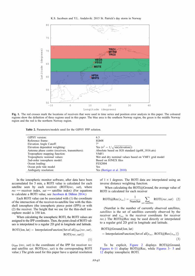
Site name Latitude Longitude GNSS receiver RTK monitor Scintillation receiverTromsø 69.540 18.940 TRO1 MTRM TRO2Vega 65.531 11.964 VEGS – VEG2Steinkjer 63.859 11.502 – MSTE –Hønefoss 59.980 10.249 HFS4 MHFS –

J. Space Weather Space Clim., 6, A9 (2016)

A9-p2

In the ionospheric monitor software, after data have beenaccumulated for 5 min, a ROTI value is calculated for eachsatellite seen by each receiver. (ROTI(rec, sat), whererec == receiver index, sat == satellite index) (For equationsto calculate a ROTI value, see Jacobsen & Dähnn 2014.)

Each ROTI value can be associated with (1) the coordinateof the intersection of the receiver-to-satellite line with the thin-shell ionosphere (the ionospheric pierce point (IPP)) or with(2) the receiver. The height that we use for the thin-shell ion-osphere model is 350 km.

When calculating the ionospheric ROTI, the ROTI values areassigned to the IPP coordinates. Then, the point cloud of ROTI val-ues is interpolated to a regular 2D grid in longitude and latitude.

ROTIðlon; latÞ ¼ InterpolationFunctionðSet of all½xIPPðrec; satÞ;ROTIðrec; satÞ�Þ

ð1Þ(xIPP (rec, sat) is the coordinate of the IPP for receiver recand satellite sat. ROTI(rec, sat) is the corresponding ROTIvalue.) The grids used for this paper have a spatial resolution

of 1 · 1 degrees. The ROTI data are interpolated using aninverse distance weighting function.

When calculating the ROTI@Ground, the average value ofROTI is calculated for each receiver

ROTI@RecðxrecÞ ¼1

NumSat

X

sat¼satellites

ROTIðrec; satÞ ð2Þ

(NumSat is the number of currently observed satellites,satellites is the set of satellites currently observed by thereceiver and xrec is the receiver coordinate for receiverrec.) The ROTI@Rec may be used directly or interpolatedto a regular grid 2D grid in longitude and latitude.

ROTI@Ground lon; latð Þ¼ InterpolationFunctionðSet of all½xrec; ROTI@RecðxrecÞ�Þ

ð3Þ

To be explicit, Figure 2 displays ROTI@Ground,Figures 6–11 display ROTI@Rec, while Figures 3– 5 and12 display ionospheric ROTI.

Fig. 1. The red crosses mark the locations of receivers that were used in time series and position error analysis in this paper. The colouredregions show the definition of three regions used in this paper. The blue area is the southern Norway region, the green is the middle Norwayregion and the red is the northern Norway region.

Table 2. Parameters/models used for the GIPSY PPP solution.

GIPSY version: 6.3Reference frame: IGb08Elevation Angle Cutoff: 7�Elevation dependent weighting: Yes (r2 ¼ 1=

ffiffiffiffiffiffiffiffiffiffiffiffiffiffiffiffiffiffiffiffiffiffiffiffiffiffiffisinðelevationÞ

p)

Antenna phase centre (receivers, transmitters): Absolute based on IGS standard (igs08_1816.atx)Troposphere mapping function: VMF1Tropospheric nominal values: Wet and dry nominal values based on VMF1 grid model2nd-order ionosphere model: Based on IONEX filesOcean loading: FES2004Ocean pole tide model YesAmbiguity resolution: Yes (Bertiger et al. 2010)

K.S. Jacobsen and Y.L. Andalsvik: 2015 St. Patrick’s day storm in Norway

A9-p3

(a)

(b)

(c)

(d)

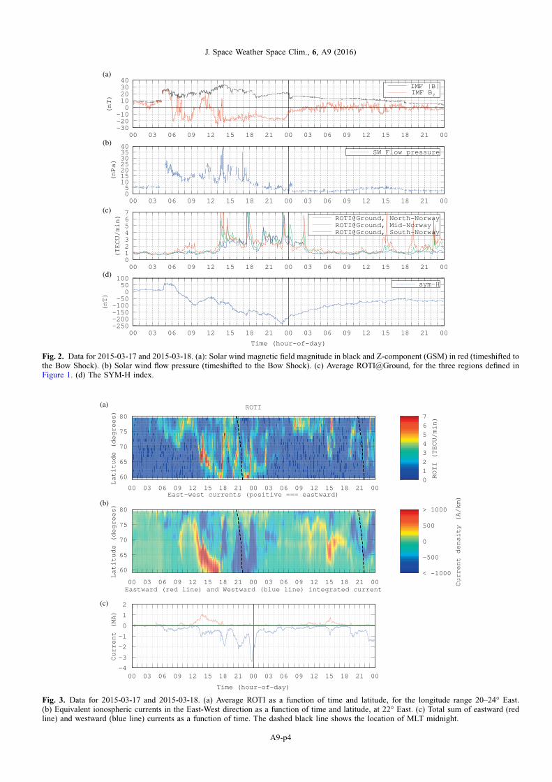
Fig. 2. Data for 2015-03-17 and 2015-03-18. (a): Solar wind magnetic field magnitude in black and Z-component (GSM) in red (timeshifted tothe Bow Shock). (b) Solar wind flow pressure (timeshifted to the Bow Shock). (c) Average ROTI@Ground, for the three regions defined inFigure 1. (d) The SYM-H index.

(a)

(b)

(c)

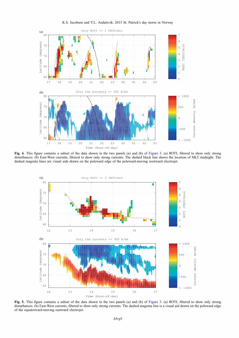
Fig. 3. Data for 2015-03-17 and 2015-03-18. (a) Average ROTI as a function of time and latitude, for the longitude range 20–24� East.(b) Equivalent ionospheric currents in the East-West direction as a function of time and latitude, at 22� East. (c) Total sum of eastward (redline) and westward (blue line) currents as a function of time. The dashed black line shows the location of MLT midnight.

J. Space Weather Space Clim., 6, A9 (2016)

A9-p4

(a)

(b)

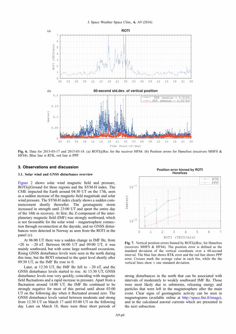
Fig. 4. This figure contains a subset of the data shown in the two panels (a) and (b) of Figure 3. (a) ROTI, filtered to show only strongdisturbances. (b) East-West currents, filtered to show only strong currents. The dashed black line shows the location of MLT midnight. Thedashed magenta lines are visual aids drawn on the poleward edge of the poleward-moving westward electrojet.

(a)

(b)

Fig. 5. This figure contains a subset of the data shown in the two panels (a) and (b) of Figure 3. (a) ROTI, filtered to show only strongdisturbances. (b) East-West currents, filtered to show only strong currents. The dashed magenta line is a visual aid drawn on the poleward edgeof the equatorward-moving eastward electrojet.

K.S. Jacobsen and Y.L. Andalsvik: 2015 St. Patrick’s day storm in Norway

A9-p5

3. Observations and discussion

3.1. Solar wind and GNSS disturbance overview

Figure 2 shows solar wind magnetic field and pressure,ROTI@Ground for three regions and the SYM-H index. TheCME impacted the Earth around 04:30 UT on the 17th, seenas a sudden increase of the magnetic field magnitude and solarwind pressure. The SYM-H index clearly shows a sudden com-mencement shortly thereafter. The geomagnetic stormincreased in strength until 23:00 UT and spent the entire dayof the 18th in recovery. At first, the Z-component of the inter-planetary magnetic field (IMF) was strongly northward, whichis not favourable for the solar wind – magnetosphere connec-tion through reconnection at the dayside, and no GNSS distur-bances were detected in Norway as seen from the ROTI in thepanel (c).

At 06:00 UT there was a sudden change in IMF Bz, from+20 to �20 nT. Between 06:00 UT and 09:00 UT, it wasmainly southward, but with some large northward excursions.Rising GNSS disturbance levels were seen in the north duringthis time, but the ROTI returned to the quiet level shortly after09:30 UT, as the IMF Bz rose to 0.

Later, at 12:30 UT, the IMF Bz fell to �20 nT, and theGNSS disturbance levels started to rise. At 13:30 UT, GNSSdisturbance levels rose very quickly, coinciding with magneticfield fluctuations and a rapid increase in pressure. Apart from afluctuation around 14:00 UT, the IMF Bz continued to bestrongly negative for most of this period until about 03:00UT on the following day when it fluctuated around zero. TheGNSS disturbance levels varied between moderate and strongfrom 12:30 UT on March 17 until 03:00 UT on the followingday. Later on March 18, there were three short periods of

strong disturbances in the north that can be associated withintervals of moderately to weakly southward IMF Bz. Thosewere most likely due to substorms, releasing energy andparticles that were left in the magnetosphere after the mainevent. Clear signs of geomagnetic activity can be seen inmagnetograms (available online at http://space.fmi.fi/image),and in the calculated auroral currents which are presented inthe next subsection.

(a)

(b)

Fig. 6. Data for 2015-03-17 and 2015-03-18. (a) ROTI@Rec for the receiver HFS4. (b) Position errors for Hønefoss (receivers MHFS &HFS4). Blue line is RTK, red line is PPP.

Fig. 7. Vertical position errors binned by ROTI@Rec, for Hønefoss(receivers MHFS & HFS4). The position error is defined as thestandard deviation of the vertical coordinate over a 60-secondinterval. The blue line shows RTK error and the red line shows PPPerror. Crosses mark the average value in each bin, while the thevertical lines show ± one standard deviation.

J. Space Weather Space Clim., 6, A9 (2016)

A9-p6

3.2. Auroral electrojet

The panel (a) of Figure 3 shows ionospheric ROTI as a func-tion of time and latitude. For each time and latitude, the valueshown is the average value of ROTI in the longitude range of20 to 24� East. Panel (b) shows the East-West component ofthe equivalent ionospheric currents at 22� East, calculatedbased on ground magnetometer measurements. The time andlatitude axes are the same as for the panel (a). Panel (c) showsthe total value (i.e. integrated over all latitudes) of the East-West currents. Strong ROTI values and strong currents wereobserved between 12:00 UT on the 17th and 01:00 UT onthe 18th.

The two panels (a) and (b) of Figure 3 clearly indicate thatthere is at least a co-variation between equivalent ionosphericcurrents and ionospheric density irregularities. However, whilethe general pattern is similar, they also clearly demonstrate thatthere is not a simple linear relationship between current densityand irregularity strength. To take a closer look at this, we madea plot focusing on the strong currents and disturbances beforeand around midnight.

Figure 4 shows a zoomed-in view of the two panels (a) and(b), for times from 17:00 UT on the 17th to 03:00 UT on the18th. The colour scales are the same as in Figure 3 but lowROTI (<3 TECU/min) and currents (<300 A/km) values arenot shown, in order to emphasize the high values. The figurereveals that the disturbed area was located at the poleward edgeof poleward-moving areas of westward current. This ismost clearly seen around 18:00 UT, 20:00 to 21:00 UT andaround 23:30 UT. The poleward edge of the electrojet islocated just equatorward of the open-closed magnetic field lineboundary.

The location of the electrojet current moving poleward is asignature that tail reconnection dominates over daysidereconnection, while an equatorward motion indicates thatreconnection at the dayside, where patches are produced, dom-inates (Cowley & Lockwood 1992; Lockwood & Cowley1992; Milan et al. 2007). Equatorward motion may also occurwithout dayside reconnection in the recovery phase of as sub-storm (Akasofu 1964, 2013). There are two consequences of

(a)

(b)

(c)

Fig. 8. Data for 2015-03-17 and 2015-03-18. (a) Phase scintillation index for all GPS and GLONASS satellites, from the scintillation receiverin Vega. (b) ROTI@Rec for the receiver VEGS. (c) Position errors for Steinkjer (RTK) and Vega (PPP) (receivers MSTE & VEGS). Blue line isRTK, red line is PPP.

Fig. 9. Vertical position errors binned by ROTI@Rec, for Steinkjer(RTK) and Vega (PPP) (receivers MSTE & VEGS). The positionerror is defined as the standard deviation of the vertical coordinateover a 60-second interval. The blue line shows RTK error and thered line shows PPP error. Crosses mark the average value in eachbin, while the the vertical lines show ± one standard deviation.

K.S. Jacobsen and Y.L. Andalsvik: 2015 St. Patrick’s day storm in Norway

A9-p7

tail reconnection that could be linked to generation of iono-spheric irregularities that are observed as increased ROTI:

– when reconnection processes are ongoing in the tail,plasma patches will convect across the open-closed mag-netic field boundary and then move on closed magneticfield lines towards the dayside;

– Energetic particle precipitation will occur in the auroraloval region. This may contribute to the structuring ofexisting patches.

Both of these phenomena would affect the region in whichthe ionospheric disturbances are observed. Unfortunately, thedata available here cannot be used to distinguish between thoseeffects. All-sky imaging data were poor or not available for thisperiod due to cloud cover. Radar data were also not availablefor this region at this time. Thus, the work to determine the rel-ative importance of those effects will have to be left to futureevents. We note that in the global view of this event in thepaper by Cherniak et al. (2015), patches were observed to driftacross the polar cap and enter the nightside auroral oval, andthey were associated with significant increases in the intensityof ionospheric irregularities. In a case study of another eventby Jin et al. (2014), patches that had entered the auroral region(auroral blobs) were directly connected to the strongest scintil-lations. In the case study by van der Meeren et al. (2015), scin-tillations were not observed for patches outside of the region ofauroral emissions/particle precipitation, but strong scintilllation

was observed in association with patches co-located withstrong auroral emissions/particle precipitation. In-situ observa-tions of patches by Moen et al. (2012) indicate that particleprecipitation is a driver of plasma instabilities that form struc-tures on scales that cause scintillation in GNSS signals.

(a)

(b)

(c)

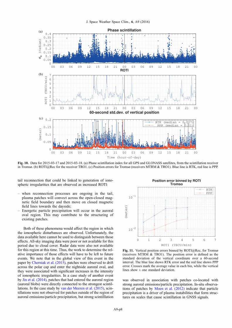
Fig. 10. Data for 2015-03-17 and 2015-03-18. (a) Phase scintillation index for all GPS and GLONASS satellites, from the scintillation receiverin Tromsø. (b) ROTI@Rec for the receiver TRO1. (c) Position errors for Tromsø (receivers MTRM & TRO1). Blue line is RTK, red line is PPP.

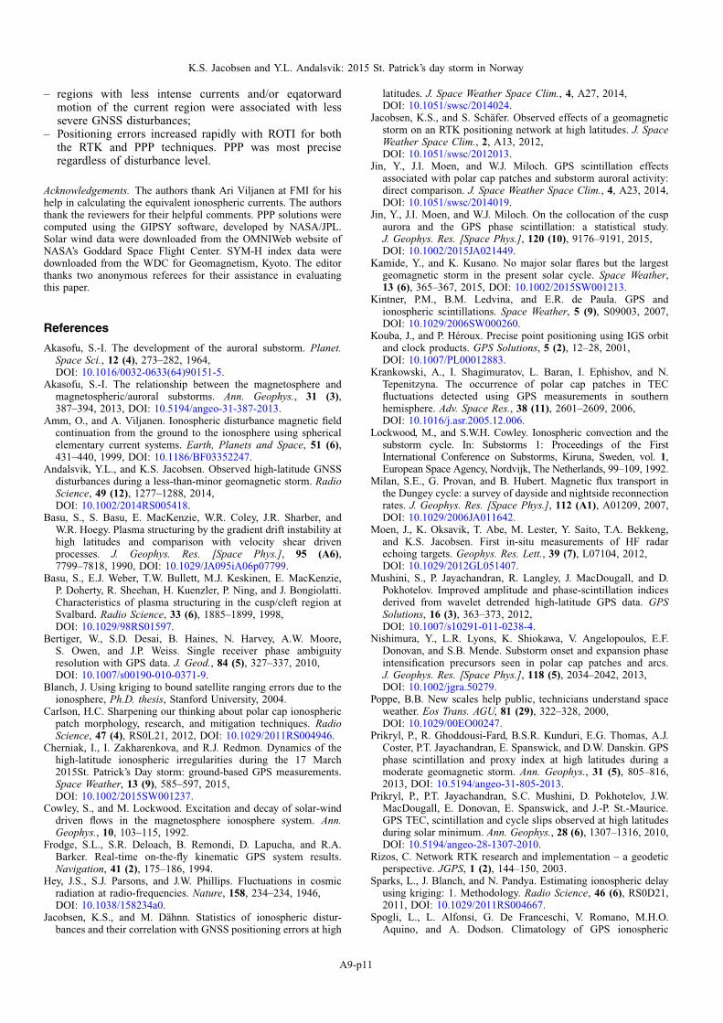
Fig. 11. Vertical position errors binned by ROTI@Rec, for Tromsø(receivers MTRM & TRO1). The position error is defined as thestandard deviation of the vertical coordinate over a 60-secondinterval. The blue line shows RTK error and the red line shows PPPerror. Crosses mark the average value in each bin, while the verticallines show ± one standard deviation.

J. Space Weather Space Clim., 6, A9 (2016)

A9-p8

Figure 5 shows a zoomed-in view for 12:00 to 17:00 UT onthe 17th, the time period that had a strong eastward current.Between 13:30 and 14:10 UT, the disturbed area is locatedbetween the region of eastward and westward currents, andthe current regions as well as the disturbed region are alternat-ing between poleward and equatorward motion. The combina-tion of several concurrent effects makes the analysis of thistime period complicated. Without other supporting non-GNSS measurements, the different phenomena cannot beconclusively identified and separated. From 14:30 to 15:30,the large ROTI values are located on the poleward edge ofthe equatorward-moving eastward current. However, this isnot observed for the times 12:30 to 13:30 UT and 15:30 to17:00 UT. We were not able to come to a conclusion regard-ing the physical mechanisms responsible for this behaviour,so we only make a note of this behaviour here and intendto return to this topic during investigations of future events.

3.3. Position errors

Figures 6, 8 and 10 show time series of phase scintillation(where available), ROTI and position errors for the southern,middle and northern Norway regions, respectively. In Figures 6and 10, the receivers (GNSS, RTK monitor, scintillation) usedare co-located, but for Figure 8 this was not possible. TheRTK monitor receiver MSTE, which is used for the RTK coor-dinates, is approximately 180 km south of the other receiversshown in Figure 1 and approximately 14 km away from the clos-est RTK network receiver. This is still close enough for the timeseries comparisons to be valid, but it may suffer from additionalerrors due to its separation from the RTK network receivers,whereas the receivers at Hønefoss and Tromsø are co-locatedwith a RTK network receiver.

To determine how the position errors vary with the iono-spheric disturbances, they were sorted by the ROTI@Rec.

(a)

(b) (c)

Fig. 12. Maps of phase scintillation, VTEC and ROTI for the time period 17:40–17:45 UT on March 17th. (a) Phase scintillation, (b) verticalTEC, (c) ROTI.

K.S. Jacobsen and Y.L. Andalsvik: 2015 St. Patrick’s day storm in Norway

A9-p9

The bin size was 1 ROTI, and the values were not calculated forbins with less than 20 data points. In each bin, the mean valueand the standard deviation were calculated. Figures 7, 9 and 11show the results. In Figure 9 PPP have results for higher ROTIthan RTK. This is because the RTK processing was unable toprovide enough coordinates when ROTI was at its highest lev-els. The effect can also be seen in Figure 8 by close examinationof the time series, where there are fewer data points (blue dots)in the panel (c) during periods of high activity.

Hønefoss, which is located at 60� North, is generally unaf-fected by activity in the auroral oval during weak to moderateevents, as the auroral oval is too far north to affect it. Thisevent, however, was strong enough to expand the auroral ovalso far south that even Hønefoss was impacted by the fulleffects of the storm at night on the 17th. Figure 6 shows thetime series of ROTI and position errors. A strong response isseen in both ROTI and position errors between 12 UT on the17th and 3 UT on the 18th. An increased level of error is alsoseen in the RTK coordinates in the hours prior to 12 UT, with-out any corresponding signature in the ROTI or PPP error. Thelikely cause of this are increased plasma gradients which causedifficulties for the network RTK processing, but which do notcontain strong structuring at small scales. This could be causedby patches that are not structured at small scales.

Vega and Steinkjer are sites in the middle of Norway. Mod-erate or stronger geomagnetic storms tend to expand the auroraloval enough to disturb these sites. Figure 8 shows the time ser-ies of ROTI and position errors. As for Hønefoss, disturbancesare observed between 12 UT on the 17th and 3 UT on the 18th.There are some position errors observed for RTK at around 9UT, coinciding with some observations of low level phase scin-tillation and slightly enhanced ROTI. The PPP position does notshow a visible increase in error at that time. There are also somesmall signs of disturbances at the end of the 18th.

Tromsø, at 70� North, is located beneath the auroral oval atnight during normal conditions and thus frequently experiencesionospheric disturbances. Figure 10 shows the time series ofROTI and position errors. Like the other sites, it experiencedmoderate to strong disturbances between 12 UT on the 17thand 3 UT on the 18th, and some disturbances around 9 UT.Scintillations were observed around 9 UT, and these werestronger than those observed in the middle of Norway at thesame time. An enhanced level of ROTI was also observed atthat time, rising gradually from 6 to 9 UT, peaking around 9UT and then falling back down to the quiet level. Tromsøwas the only one of the three sites to experience significantpositioning errors late on the 18th.

All of the sites observed short-lived peaks of the ROTI,coinciding with peaks in phase scintillation activity. The timingof the peaks corresponds to the times of intensified electrojetcurrents and poleward motion, or in some cases motion whosedirection was unclear, of the current region. This means thatthe most intense disturbances, whether measured by ROTI orphase scintillation, were caused by substorms that result fromactive tail reconnection. This can be seen in Figures 3 and 4and was discussed in the previous section.

Figures 7, 9 and 11 show the relation between ROTI andpositioning errors. All of them show the same pattern of posi-tioning errors increasing rapidly with increasing ROTI. Thecurves for the RTK and PPP techniques appear to be approx-imately parallel, meaning that the PPP technique yields moreprecise coordinates than RTK regardless of the ionospheric dis-turbance level.

3.4. Scintillation example

Figure 12 shows phase scintillation measurements from NMA’sscintillation receiver network, and simultaneous maps ofVTEC and ROTI for the same geographical area. The scintil-lation receivers were located in Bjørnøya, Bodø, The FaroeIslands, Honningsvåg, Hopen, Jan Mayen, Kautokeino,Ny-Ålesund, Tromsø and Vega, and are plotted as green dia-monds in panel (a). In panel (a), the GPS and GLONASSphase scintillation indices are plotted individually for eachscintillation measurement. The size of the circles is propor-tional to the strength of the scintillation. To show the scale,below the plot three circles are drawn along with the corre-sponding scintillation values in radians. The plot contains datafrom 5 min of measurements. The scintillation index is calcu-lated once per minute, so there are five data points for eachsatellite link. Scintillation measurements from satellites below15� elevation are not plotted. Panels (b) and (c) show the totalelectron content and ionospheric ROTI maps, respectively. TheVTEC map was produced by Kriging interpolation of theVTEC values at the IPPs. Information about the Kriging tech-nique, and how it can be applied to ionospheric VTEC, can befound in e.g. Blanch (2004) and Sparks et al. (2011). The scalesof the VTEC and ROTI maps have been adjusted to best showthe anomalous conditions. For reference, a normal quiet-timelevel of ROTI is around 1 TECU/min, a normal peak daytimeVTEC for southern Norway at this time of year is between 20and 30 TECU, and a normal nighttime VTEC is around 5 TECU.

The strong phase scintillations are located in the area ofenhanced (>3) ROTI, but they are not showing a preferencefor the area of very high (>7) ROTI. There is a lot of variationboth spatially and temporally for the scintillation index. Thismay indicate that the scintillation is caused by smaller struc-tures within the area of enhanced ROTI. Almost the entire areacontains higher than normal values of VTEC, but the area inwhich there are very high ROTI values has particularly highVTEC values. The area of maximum VTEC value in the lowerleft corner of the plot is the edge of the region of sunlit plasma,and is not related to the space weather event. The amount ofTEC is too high to have been produced locally, so transportof plasma from the dayside must have occurred. Within theregion of very high VTEC values between 60 and 65� Norththere are most likely plasma patches. The resolution of theTEC map may not be sufficient to fully characterize the shapeof individual patches, but the uneven distribution and highVTEC values seen in the plot are a strong indication thatplasma patches are present in the area.

4. Conclusions

We have presented our observations of the 2015 St. Patrick’sday geomagnetic storm. These are our main conclusions:

– strong GNSS disturbances were observed at all latitudes inNorway on March 17th and early on the 18th. Late on the18th, strong disturbances were only observed in the north-ern parts of Norway;

– GNSS disturbances, measured by ROTI, were mostintense on the poleward edge of poleward-moving electro-jet currents. This is possibly related to patches and/or par-ticle precipitation activity caused by active tailreconnection. The relative importance of these phenom-ena, or the importance of having both simultaneously, can-not be determined from our data;

J. Space Weather Space Clim., 6, A9 (2016)

A9-p10

– regions with less intense currents and/or eqatorwardmotion of the current region were associated with lesssevere GNSS disturbances;

– Positioning errors increased rapidly with ROTI for boththe RTK and PPP techniques. PPP was most preciseregardless of disturbance level.

Acknowledgements. The authors thank Ari Viljanen at FMI for hishelp in calculating the equivalent ionospheric currents. The authorsthank the reviewers for their helpful comments. PPP solutions werecomputed using the GIPSY software, developed by NASA/JPL.Solar wind data were downloaded from the OMNIWeb website ofNASA’s Goddard Space Flight Center. SYM-H index data weredownloaded from the WDC for Geomagnetism, Kyoto. The editorthanks two anonymous referees for their assistance in evaluatingthis paper.

References

Akasofu, S.-I. The development of the auroral substorm. Planet.Space Sci., 12 (4), 273–282, 1964,DOI: 10.1016/0032-0633(64)90151-5.

Akasofu, S.-I. The relationship between the magnetosphere andmagnetospheric/auroral substorms. Ann. Geophys., 31 (3),387–394, 2013, DOI: 10.5194/angeo-31-387-2013.

Amm, O., and A. Viljanen. Ionospheric disturbance magnetic fieldcontinuation from the ground to the ionosphere using sphericalelementary current systems. Earth, Planets and Space, 51 (6),431–440, 1999, DOI: 10.1186/BF03352247.

Andalsvik, Y.L., and K.S. Jacobsen. Observed high-latitude GNSSdisturbances during a less-than-minor geomagnetic storm. RadioScience, 49 (12), 1277–1288, 2014,DOI: 10.1002/2014RS005418.

Basu, S., S. Basu, E. MacKenzie, W.R. Coley, J.R. Sharber, andW.R. Hoegy. Plasma structuring by the gradient drift instability athigh latitudes and comparison with velocity shear drivenprocesses. J. Geophys. Res. [Space Phys.], 95 (A6),7799–7818, 1990, DOI: 10.1029/JA095iA06p07799.

Basu, S., E.J. Weber, T.W. Bullett, M.J. Keskinen, E. MacKenzie,P. Doherty, R. Sheehan, H. Kuenzler, P. Ning, and J. Bongiolatti.Characteristics of plasma structuring in the cusp/cleft region atSvalbard. Radio Science, 33 (6), 1885–1899, 1998,DOI: 10.1029/98RS01597.

Bertiger, W., S.D. Desai, B. Haines, N. Harvey, A.W. Moore,S. Owen, and J.P. Weiss. Single receiver phase ambiguityresolution with GPS data. J. Geod., 84 (5), 327–337, 2010,DOI: 10.1007/s00190-010-0371-9.

Blanch, J. Using kriging to bound satellite ranging errors due to theionosphere, Ph.D. thesis, Stanford University, 2004.

Carlson, H.C. Sharpening our thinking about polar cap ionosphericpatch morphology, research, and mitigation techniques. RadioScience, 47 (4), RS0L21, 2012, DOI: 10.1029/2011RS004946.

Cherniak, I., I. Zakharenkova, and R.J. Redmon. Dynamics of thehigh-latitude ionospheric irregularities during the 17 March2015St. Patrick’s Day storm: ground-based GPS measurements.Space Weather, 13 (9), 585–597, 2015,DOI: 10.1002/2015SW001237.

Cowley, S., and M. Lockwood. Excitation and decay of solar-winddriven flows in the magnetosphere ionosphere system. Ann.Geophys., 10, 103–115, 1992.

Frodge, S.L., S.R. Deloach, B. Remondi, D. Lapucha, and R.A.Barker. Real-time on-the-fly kinematic GPS system results.Navigation, 41 (2), 175–186, 1994.

Hey, J.S., S.J. Parsons, and J.W. Phillips. Fluctuations in cosmicradiation at radio-frequencies. Nature, 158, 234–234, 1946,DOI: 10.1038/158234a0.

Jacobsen, K.S., and M. Dähnn. Statistics of ionospheric distur-bances and their correlation with GNSS positioning errors at high

latitudes. J. Space Weather Space Clim., 4, A27, 2014,DOI: 10.1051/swsc/2014024.

Jacobsen, K.S., and S. Schäfer. Observed effects of a geomagneticstorm on an RTK positioning network at high latitudes. J. SpaceWeather Space Clim., 2, A13, 2012,DOI: 10.1051/swsc/2012013.

Jin, Y., J.I. Moen, and W.J. Miloch. GPS scintillation effectsassociated with polar cap patches and substorm auroral activity:direct comparison. J. Space Weather Space Clim., 4, A23, 2014,DOI: 10.1051/swsc/2014019.

Jin, Y., J.I. Moen, and W.J. Miloch. On the collocation of the cuspaurora and the GPS phase scintillation: a statistical study.J. Geophys. Res. [Space Phys.], 120 (10), 9176–9191, 2015,DOI: 10.1002/2015JA021449.

Kamide, Y., and K. Kusano. No major solar flares but the largestgeomagnetic storm in the present solar cycle. Space Weather,13 (6), 365–367, 2015, DOI: 10.1002/2015SW001213.

Kintner, P.M., B.M. Ledvina, and E.R. de Paula. GPS andionospheric scintillations. Space Weather, 5 (9), S09003, 2007,DOI: 10.1029/2006SW000260.

Kouba, J., and P. Héroux. Precise point positioning using IGS orbitand clock products. GPS Solutions, 5 (2), 12–28, 2001,DOI: 10.1007/PL00012883.

Krankowski, A., I. Shagimuratov, L. Baran, I. Ephishov, and N.Tepenitzyna. The occurrence of polar cap patches in TECfluctuations detected using GPS measurements in southernhemisphere. Adv. Space Res., 38 (11), 2601–2609, 2006,DOI: 10.1016/j.asr.2005.12.006.

Lockwood, M., and S.W.H. Cowley. Ionospheric convection and thesubstorm cycle. In: Substorms 1: Proceedings of the FirstInternational Conference on Substorms, Kiruna, Sweden, vol. 1,European Space Agency, Nordvijk, The Netherlands, 99–109, 1992.

Milan, S.E., G. Provan, and B. Hubert. Magnetic flux transport inthe Dungey cycle: a survey of dayside and nightside reconnectionrates. J. Geophys. Res. [Space Phys.], 112 (A1), A01209, 2007,DOI: 10.1029/2006JA011642.

Moen, J., K. Oksavik, T. Abe, M. Lester, Y. Saito, T.A. Bekkeng,and K.S. Jacobsen. First in-situ measurements of HF radarechoing targets. Geophys. Res. Lett., 39 (7), L07104, 2012,DOI: 10.1029/2012GL051407.

Mushini, S., P. Jayachandran, R. Langley, J. MacDougall, and D.Pokhotelov. Improved amplitude and phase-scintillation indicesderived from wavelet detrended high-latitude GPS data. GPSSolutions, 16 (3), 363–373, 2012,DOI: 10.1007/s10291-011-0238-4.

Nishimura, Y., L.R. Lyons, K. Shiokawa, V. Angelopoulos, E.F.Donovan, and S.B. Mende. Substorm onset and expansion phaseintensification precursors seen in polar cap patches and arcs.J. Geophys. Res. [Space Phys.], 118 (5), 2034–2042, 2013,DOI: 10.1002/jgra.50279.

Poppe, B.B. New scales help public, technicians understand spaceweather. Eos Trans. AGU, 81 (29), 322–328, 2000,DOI: 10.1029/00EO00247.

Prikryl, P., R. Ghoddousi-Fard, B.S.R. Kunduri, E.G. Thomas, A.J.Coster, P.T. Jayachandran, E. Spanswick, and D.W. Danskin. GPSphase scintillation and proxy index at high latitudes during amoderate geomagnetic storm. Ann. Geophys., 31 (5), 805–816,2013, DOI: 10.5194/angeo-31-805-2013.

Prikryl, P., P.T. Jayachandran, S.C. Mushini, D. Pokhotelov, J.W.MacDougall, E. Donovan, E. Spanswick, and J.-P. St.-Maurice.GPS TEC, scintillation and cycle slips observed at high latitudesduring solar minimum. Ann. Geophys., 28 (6), 1307–1316, 2010,DOI: 10.5194/angeo-28-1307-2010.

Rizos, C. Network RTK research and implementation – a geodeticperspective. JGPS, 1 (2), 144–150, 2003.

Sparks, L., J. Blanch, and N. Pandya. Estimating ionospheric delayusing kriging: 1. Methodology. Radio Science, 46 (6), RS0D21,2011, DOI: 10.1029/2011RS004667.

Spogli, L., L. Alfonsi, G. De Franceschi, V. Romano, M.H.O.Aquino, and A. Dodson. Climatology of GPS ionospheric

K.S. Jacobsen and Y.L. Andalsvik: 2015 St. Patrick’s day storm in Norway

A9-p11

scintillations over high and mid-latitude European regions. Ann.Geophys., 27 (9), 3429–3437, 2009,DOI: 10.5194/angeo-27-3429-2009.

Tiwari, R., F. Ghafoori, O. Al-Fanek, O. Haddad, and S. Skone.Investigation of high latitude ionospheric scintillationsobserved in the Canadian region, in: Proceedings of the 23rdInternational Technical Meeting of the Satellite Division of theInstitute of Navigation (ION GNSS 2010), Portland, OR,349–360, 2010.

van der Meeren, C., K. Oksavik, D.A. Lorentzen, M.T. Rietveld, andL.B.N. Clausen. Severe and localized GNSS scintillation at thepoleward edge of the nightside auroral oval during intensesubstorm aurora. J. Geophys. Res. [Space Phys.], 120,10607–10621, 2015, DOI: 10.1002/2015JA021819.

Weber, E.J., J.A. Klobuchar, J. Buchau, H.C. Carlson, R.C.Livingston, O. de la Beaujardiere, M. McCready, J.G. Moore,and G.J. Bishop. Polar cap F layer patches: Structure anddynamics. J. Geophys. Res. [Space Phys.], 91 (A11),12121–12129, 1986, DOI: 10.1029/JA091iA11p12121.

Zou, Y., Y. Nishimura, L.R. Lyons, E.F. Donovan, J.M. Ruohoniemi,N. Nishitani, and K.A. McWilliams. Statistical relationshipsbetween enhanced polar cap flows and PBIs. J. Geophys. Res.[Space Phys.], 119 (1), 151–162, 2014,DOI: 10.1002/2013JA019269.

Zumberge, J.F., M.B. Heflin, D.C. Jefferson, M.M. Watkins, andF.H. Webb. Precise point positioning for the efficient and robustanalysis of GPS data from large networks. J. Geophys. Res. [SolidEarth], 102 (B3), 5005–5017, 1997, DOI: 10.1029/96JB03860.

Cite this article as: Jacobsen K.S. & Andalsvik Y.L. Overview of the 2015 St. Patrick’s day storm and its consequences for RTK andPPP positioning in Norway. J. Space Weather Space Clim., 6, A9, 2016, DOI: 10.1051/swsc/2016004.

J. Space Weather Space Clim., 6, A9 (2016)

A9-p12