p-cao fail · monte carlo bias estimations was very small, and the distributions of the bias...

DOCUMENT RESUME

ED 422 390 TM 028 952

AUTHOR Thompson, Bruce; Fan, XitaoTITLE Bootstrap Estimation of Sample Statistic Bias in Structural

Equation Modeling.PUB DATE 1998-04-00NOTE 40p.; Paper presented at the Annual Meeting of the American

Educational Research Association (San Diego, CA, April13-17, 1998).

PUB TYPE Reports - Evaluative (142) Speeches/Meeting Papers (150)EDRS PRICE MF01/PCO2 Plus Postage.DESCRIPTORS *Estimation (Mathematics); Goodness of Fit; Monte Carlo

Methods; Sample Size; *Statistical Bias; *StructuralEquation Models

IDENTIFIERS *Bootstrap Methods

ABSTRACTThis study empirically investigated bootstrap bias

estimation in the area of structural equation modeling (SEM). Three correctlyspecified SEM models were used under four different sample size conditions.Monte Carlo experiments were carried out to generate the criteria againstwhich bootstrap bias estimation should be judged. For SEM fit indices, biasestimates from the bootstrap and Monte Carlo experiments were quitecomparable in most cases. It is noted that bias was constrained in onedirection in the Monte Carlo experiments because of the perfect fit of thetrue SEM models. For the SEM loadings and coefficients, the differencebetween bootstrap and Monte Carlo bias estimations was very small, and thedistributions of the bias estimators from "the two experiments were quitesimilar. For the SEM variances/covariances, the comparison of the biasestimator distributions from the two experiments indicated that bootstrapbias estimation could be considered adequate. Because the study involvedthree SEM models which served as an internal replication mechanism, thelikelihood of chance discovery for the findings was small, and the findingsshould have reasonable generalizability. Future studies may extend thecurrent findings by examining misspecified SEM models. Data nonnormality maybe another dimension to be considered in future investigations. (Contains 6figures, 4 tables, and 40 references.) (Author)

********************************************************************************

Reproductions supplied by EDRS are the best that can be madefrom the original document.

********************************************************************************

BTRAPSEM.DOC

BOOTSTRAP ESTIMATION OF SAMPLE STATISTIC BIAS

IN STRUCTURAL EQUATION MODELING

PERMISSION TO REPRODUCE ANDDISSEMINATE THIS MATERIAL HAS

BEEN GRANTED BY

\P-"cao_FAil

TO THE EDUCATIONAL RESOURCESINFORMATION CENTER (ERIC)

1

Xitao Fan

Utah State University

Bruce Thompson

Texas A&M Universityand

Baylor College of Medicine

Running Head: Bootstrap Bias Estimation in SEM

U.S. DEPARTMENT OF EDUCATIONOffice of Educational Research and Improvement

EDUCATIONAL RESOURCES INFORMATIONCENTER (ERIC)

I-his document has been reproduced asreceived from the person or organizationoriginating it.

0 Minor changes have been made toimprove reproduction quality.

Points of view or opinions stated in thisdocument do not necessarily representofficial OERI position or policy.

Note: Correspondence about this paper should be sent to the first author at: Dept. ofPsychology, Utah State University, Logan, UT 84322-2810. Phone: (435)797-1451, and

E-Mail: [email protected]

Paper presented at the 1998 Annual Meeting of the American Educational Research

Association, San Diego, CA, April 13-17 (Session #: 15.51).

2

Bootstrap Bias Estimation in SEM 2

ABSTRACT

This study empirically investigated bootstrap bias estimation in the area of structural

equation modeling. Three correctly specified SEM models were used under four different sample

size conditions. Monte Carlo experiments were carried out to generate the criteria against which

bootstrap bias estimation could be judged. For SEM fit indices, bias estimateS from the bootstrap

and Monte Carlo experiments were quite comparable for most of them It is noted that bias was

constrained in one direction in the Monte Carlo experiments because of the perfect fit of the true

SEM models. For the SEM loadings and coefficients, the difference between bootstrap and

Monte Carlo bias estimations was very small, and the distributions of the bias estimators from the

two experiments were quite similar. For the SEM variances/covariances, the comparison of the

bias estimator distributions from the two experiments indicated that bootstrap bias estimation

could be considered adequate. Because the study involved three SEM models which served as

internal replication mechanism, the likelihood of chance discovery for the findings was small, and

the findings should have reasonable generalizability. Future studies may extend the current

findings by examining misspecified SEM models. Data non-normality may be another dimension

to be considered in future investigation.


Structural equation modeling (SEM) has increasingly been seen as a useful quantitative

technique for specifying, estimating, and testing hypothesized models describing relationships

among a set of substantively meaningful variables. Much of SEM's attractiveness is due to the

method's applicability in a wide variety of research situations, a versatility that has been amply

demonstrated (e.g., Bollen & Long, 1993; Byrne, 1994; Joreskog & SOrbom, 1989; Loehlin,

1992; SAS Institute, 1990).

Furthermore, many widely used statistical techniques may also be considered as special

cases of SEM, including regression analysis, canonical correlation analysis, confirmatory factor

analysis, and path analysis (Bagozzi, Fornell & Larcker, 1981; Bentler, 1992; Fan, 1996; Joreskog

& Sörbom, 1989). Because of such generality, SEM has been heralded as a unified model which

joins methods from econometrics, psychometrics, sociometrics, and multivariate statistics

(Bentler, 1994). In short, for researchers in the social and behavioral sciences, SEM has become

an important tool for testing theories with both experimental and non-experimental data (Bentler

& Dudgeon, 1996).

Bootstrap method, on the other hand, has also been applauded as one of the newest

breakthroughs in statistics (Kots & Johnson, 1992). The significance of bootstrapping as a

versatile nonparametric statistical approach to data analysis has been widely recognized not only

by those in the area of statistics, but also by quantitative researchers in social and behavioral

sciences. In the area of education, the recognition for the bootstrapping method was evidenced

by the invited keynote address delivered by the pioneer in bootstrapping, Bradley Efron, at the

1995 AERA Annual Meeting (Efron, 1995).

In social and behavioral sciences, bootstrap method has been used in a variety of research

situations, and for many different statistical techniques. For example, bootstrap method has been

4


applied in psychological measurement for such issues as differential test predictive validity (e.g.,

Fan & Mathews, 1994) and item bias (e.g., Harris & Kolen, 1991), and in sociological research

(e.g., Stine, 1989). The application of bootstrapping method has involved many different

statistical techniques, including correlation analysis (e.g., Rasmussen, 1987), regression analysis

(e.g., Fan & Jacoby, 1995), discriminant analysis (e.g., Dalgleish, 1994), canonical correlation

analysis (e.g., Fan & Wang, 1996), factor analysis (e.g., Lambert, Wildt, & Durand, 199;

Thompson, 1988) , and structural equation modeling (e.g., Bollen & Stine, 1990). In addition to

its original use as a nonparametric alternative to statistical significance testing (Efron, 1985),

bootstrap technique has also been advocated as a method ofinternal replication to assess the

replicability of results of an individual study (Thompson, 1993).

As a general nonparametric technique, the application ofbootstrap may be most

appropriate in situations where the statistical theory is weak, or where theoretical assumptions are

unlikely to be tenable. Structural equation modeling can be considered as an area in which the

statistical theory is relatively weak (e.g., no theoretical sampling distributions for many model fit

indices), and in which theoretical assumptions are often untenable (e.g., multivariate normality is

often violated). Viewed inn this perspective, the application of bootstrap method in SEM can be

considered quite relevant and desirable.

It has been observed that the application of bootstrap in SEM could be categorized for

four different purposes: (1) to estimate bias of sample statistic (bias estimation), (2) to estimate

standard errors, (3) to construct confidence intervals, and (4) to test SEM models (Yung &

Bentler, 1996). Despite its conceptual and procedural simplicity, and its versatility in a variety of

statistical situations, the success of applying bootstrap method as originally proposed (Efron,

'4979) in SEM may not be guaranteed. For example, it has been shown that bootstrap application'

5


(as originally defined) has failed in the area of SEM model testing (Bollen & Stine, 1993).

Because of the uncertainty about its success in SEM, Yung and Bentler (1996) made a general

suggestion that, in the area of SEM, bootstrap results should not be blindly and indiscriminantly

trusted; instead, a particular application of bootstrapping (e.g., bias estimation) in SEM needs to

be investigated until the validity of such application has been reasonably established.

Of the four major applications of bootstrap in SEM, bias estimation (i.e., to use bootstrap-

estimated bias of a statistic to represent the true bias of that statistic) has been identified as an

area where little empirical evidence exists (Yung & Bentler, 1996). Consequently, the validity of

bootstrap-based bias estimation in SEM is largely unknown. The problem here is that no studies

have been reported which investigated bootstrap bias estimation for SEM. The most relevant

studies which investigated bootstrap-based bias estimation actually applied bootstrap in

exploratory factor analysis models, but not SEM models per se.

Chatterjee (1984), based on the empirical results from exploratory factor analysis,

concluded that the bootstrap-estimated bias was very small for loadings in eiploratory factor

analysis. The results of the study, however, may not be very meaningful, for the reason that there

was no external criterion against which the validity of the bootstrap-based bias estimation could

be judged; instead, the researcher relied entirely on his "faith" in the bootstrap principle (Yung &

Bentler, 1996). The study by Ichikawa and Konishi (1995) provided the needed external criteria

("true" bias estimation empirically obtained through Monte Carlo simulation) for judging the

adequacy of bootstrap-based bias estimation. Their results indicated that bootstrap-based bias

estimation worked well for rotated factors, but less well for unrotated factors. Although this

study represents substantial improvement over that of Chatterjee (1984), the fact that both studies

investigated exploratory factor analysis, not confirmatory factor'analysis or full SEM models,

6


considerably limited the generalizability of their results for SEM. As discussed by Yung and

Bentler (1996), ". . . bootstrap estimator for biases may not work equally well in all cases .... It

would seem risky indeed to have blind faith in the bootstrap principle in the hope that bootstrap

estimation of biases in the context of structural equation modeling will work out correctly." (p.

201).

In the most general form, the bias of an estimator 0 for 0 is expressed as

B(0) = e(Ô) (1)

where 0 is the population parameter of any sort, 0 is the sample statistic for 0, and 46, is the

deviation of the sample statistic from the population parameter 0 (i.e., O = 0 - 0), and c(k) is the

expected value of DA. In an application, the true bias of the statistic B(0) is usually estimated

through Monte Carlo simulation. When N samples are drawn from the specified population, we

have each individual sample statistic deviation kJ. :

Aj

The bias of the statistic is estimated through:

B(0) = OA

vLd

(j=1, 2, 3,. . . /V)

(2)

(3)

In other words, bias estimation is the averaged value of ki obtained from repeated Monte Carlo

sampling from the defined population.

7


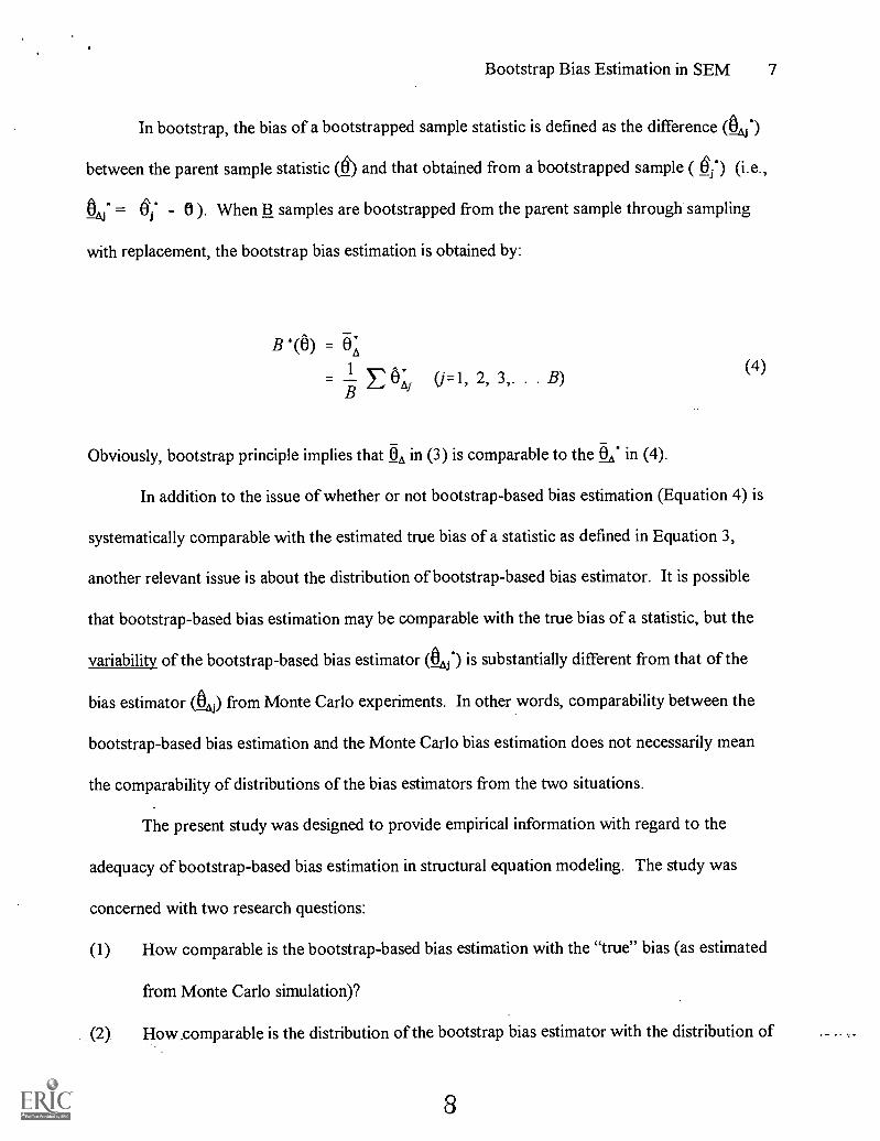
In bootstrap, the bias of a bootstrapped sample statistic is defined as the difference (0_)

between the parent sample statistic (6) and that obtained from a bootstrapped sample ( qi*) (i.e.,

- 0 ). When B samples are bootstrapped from the parent sample through sampling

with replacement, the bootstrap bias estimation is obtained by:

B *(6) = 0*A

B(j= 1, 2, 3,. . B)

(4)

Obviously, bootstrap principle implies that OA in (3) is comparable to the k. in (4).

In addition to the issue of whether or not bootstrap-based bias estimation (Equation 4) is

systematically comparable with the estimated true bias of a statistic as defined in Equation 3,

another relevant issue is about the distribution of bootstrap-based bias estimator. It is possible

that bootstrap-based bias estimation may be comparable with the true bias of a statistic, but the

variability of the bootstrap-based bias estimator (Oil) is substantially different from that of the

bias estimator (ki) from Monte Carlo experiments. In other words, comparability between the

bootstrap-based bias estimation and the Monte Carlo bias estimation does not necessarily mean

the comparability of distributions of the bias estimators from the two situations.

The present study was designed to provide empirical information with regard to the

adequacy of bootstrap-based bias estimation in structural equation modeling. The study was

concerned with two research questions:

(1) How comparable is the bootstrap-based bias estimation with the "true" bias (as estimated

from Monte Carlo simulation)?

(2) How .comparable is the distribution of the bootstrap bias estimator with the distribution of

8


the bias estimator from Monte Carlo experiments?

Both these two research questions were investigated with regard to:

(a) SEM fit indices,

(b) factor loadings and path coefficients in SEM models,

(c) variances and covariances (for both observed and latent variables) in SEM models.

METHODS

Several issues were considered in the design of this study: the generalizability of the

results of the study, the issue of sample size, and the criterion for judging the adequacy of the

bootstrap bias estimation. Attempts were made to accommodate these relevant issues in the study

design.

Increasing the Generalizability of Findings

Two features were incorporated in the study design for the purpose of increasing the

generalizability of the study results: multiple SEM models, and realistic SEM models and model

parameters. Because it is always uncertain to what extent the results from a particular SEM

model would capture the complexity of SEM modeling in general, it is possible that the findings

based on a particular model may reflect some idiosyncracies associated with the model, and

consequently, may only have limited generalizability. In this study, to minimize the possibility that

the idiosyncracies of a particular model may be mistaken for something more generalizable, three

different SEM models (one confirmatory factor analysis model and two full structural models)

with varying degrees of model complexity were simulated. Such a design of multiple models

provided a very useful mechanism for verifying the internal validity of the findings. As is generally

recognized, internal validity is the necessary, although not sufficient condition of external validity

9


(i.e., the generalizability of the findings) (Gall, Borg, & Gall, 1996).

In addition to the multiple SEM models, this study adopted realistic SEM models which

were based on substantive research studies. As suggested by Gerbing and Anderson (1993),

simulating substantively meaningful models might increase the external validity of a study. Not

only were all the three SEM models simulated in this study from substantive research studies, but

the model parameters simulated also closely matched those in the substantive studies. Of the

three SEM models simulated in this study, one is a confirmatory factor analysis model originally

appeared in the research report by Calsyn and Kenny (1977), and later discussed as a

confirmatory factor analysis model example by Joreskog and SOrbom (1989, p. 83). The second

SEM model is a full structural equation model discussed by Joreskog and Sorborn (1989, p. 178)

which was based on some longitudinal data from a study conducted by the Educational Testing

Service. The third model is also a full structural equation model which originally appeared in the

work by Wheaton, Muthdn, Alwin, and Summers (1977), and which was later widely discussed in

the SEM literature (e.g., Bentler, 1992; Joreskog & Sorbom, 1989; SAS Institute, 1990). To

limit the scope of the study, only statistically true models are simulated, although, ideally, models

with model specification error should also be studied in the future. Figure 1, Figure 2, and Figure

3 present the three SEM models used in this study, and their respective model parameters in

LISREL terms.

Insert Figure 1, 2, 3 about here

Sample Size

It is unclear how large a sample should be in SEM applications. The research findings on

1 0


this issue are inconclusive (Mac Callum, Roznowski, & Necowitz, 1992; Tanaka, 1987). It has

been reported that small sample size led to not only untrustworthy estimation results and fit

indices, but also the high rate of improper solutions in simulation (Ichikawa & Konishi, 1995).

Sample size of 200 in SEM applications has been considered as being relatively small by many

(Boomsma, 1982; Camstra & Boomsma, 1992; Ichikawa & Konishi, 1995; MacCallum, et al.,

1992). Some researchers even consider sample sizes in the thousands to be adequate (e.g., Hu,

Bentler, & Kano, 1992; Marsh et al., 1988). Realistically, however, such large sample sizes are

often beyond the reach of most researchers. Also, as pointed out by many researchers, it may not

be realistic to suggest a single value to define a small or large sample, because models and the

number of free parameters vary from application to application, so consideration of sample size

should be related to model complexity and the number of free parameters (MacCallum et al.,

1992; Tanaka, 1987).

In this study, four sample size conditions (n=100, 200, 500, 1000) were simulated. As

discussed above, there are no objective criteria on this issue. Based on our experience and our

perception about the current practice in this area, we felt that these sample size conditions were

quite representative of the current practice, and the four sample size conditions were also

considered to be reasonably spaced.

"True" Bias as the Criteria for Judging Bootstrap Bias Estimation

As discussed in the literature review section, in order to understand the adequacy of

bootstrap bias estimation, external criteria must first be obtained against which bootstrap bias

estimation can be compared. In this study, the external criteria ("true" bias) were obtained

empirically through Monte Carlo simulation. The three SEM models, the four sample size

conditions, and 200 replications within.each cell made up a total of 2400 (3 x4 x200 = 2400)

1 1


random samples to be fitted to one of the three SEM models. Based on the Monte Carlo

experiments, "true" bias for an SEM statistic ( ) was empirically obtained through Equations 2

and 3.

Within each cell condition described above, one sample was generated to served as the

parent sample for bootstrapping, and 200 samples were bootstrapped from this parent sample

using "completely nonparametric bootstrap" approach (Yung & Bentler, 1996). In this bootstrap

phase of the study, a total of 2400 samples were obtained through bootstrapping resampling, and

fitted to one of the three SEM models. The bootstrap bias estimation for the statistic (e) was

obtained through Equation 4. The Monte Carlo bias estimate B(0) and the bootstrap bias

estimate 13* were empirically compared to check if the bootstrap bias estimation 13*(&) was

systematically different than the Monte Carlo bias estimate B(6). In addition, the sampling

distribution of the bootstrap bias estimator (ki*) was compared with that of the Monte Carlo bias

estimator (k) to check how comparable the bias estimator distributions were.

Data generation was accomplished by using the SAS norrrial data generator. Multivariate

normal data were simulated using the matrix decomposition procedure (Kaiser & Dickman,

1962). All data generation, bootstrap resampling, model fitting (SAS PROC CALIS) were

accomplished through the SAS system (SAS Version 6.11).

RESULTS AND DISCUSSIONS

Because the amount of results which could be presented was huge, our presentation of the

results was selective, and we tried to focus on the main questions. Because all the simulation

results have been saved, some additional analyses can be conducted if there is enough interest.

Our presentation of the results and the related discussion followed the order of the research

12


questions presented earlier in the paper.

Comparability between Bootstrap Bias Estimation and Monte Carlo Bias Estimation

The first research question asks, "How comparable is the bootstrap bias estimation with

the "true" bias in SEM?" To answer this question, we presented the results separately for (1)

SEM fit indices; (2) loadings and path coefficients in SEM; and (3) variances and covariances in

SEM (for both observed and latent variables).

SEM fit indices. Table 1 presents the bootstrap bias estimation [13*(6)] and the Monte

Carlo bias estimation [B(6)] for a variety of SEM fit indices. A negative sign indicates a

downward bias (the estimate smaller than the parameter), and a positive sign (no sign) indicates

an upward bias (the estimate larger than the parameter). A close look at the table reveals several

observations. First, both the bootstrap and the Monte Carlo has downward bias for all the fit

indices except the x2 and the RMR (root mean square residual), for which there is upward bias.

For Monte Carlo results, this is expected, because all the models are true models, and the fit for

the defined population is perfect. In other words, for true SEM models, the population parameter

values of these indices function either as the "ceiling" (all except x2 and RMR) or the "floor" (x2

and RMR) of the possible values of the statistics. As such, bias of the statistic is constrained to be

in one direction only: doWnward (for fit indices with a "ceiling") or upward (for indices with a

"floor").

The fact that the bootstrap bias estimation is consistently in the same direction as the

"true" bias (from the Monte Carlo results) for all the fit indices is somewhat remarkable. This is

because, as Bollen and Stine (1993) discussed, the bootstrap resampling space (i.e., the bootstrap

parent sample) does not represent the null model (i.e., the correctly specified true model). This

fact means that, for these fit4ndices, the bootstrap parent sample statistic may not function as the

13


"ceiling" or "floor", as the population parameters do in Monte Carlo simulation; and some

bootstrapped samples may have better fit index values than those of the parent sample. In spite of

the difference in this regard, bootstrap still produces bias estimation consistent in direction with

the Monte Carlo estimated bias.

The second observation from Table 1 is that, for most of the fit indices, bootstrap bias

estimation is also quite comparable in magnitude with the Monte Carlo estimated bias, probably

with the exception of RIvIR, CFI, CENTRA, NNFI, and DELTA2. The comparability in

magnitude for x2, GFI, AGFI, NFI, RH01, PGFI, and PARMS are quite remarkable. The other

five indices, however, showed less comparability between the two kinds of experiments. Of these

five fit indices, bootstrap estimated bias is consistently smaller in magnitude than the bias from the

Monte Carlo experiments for RMR, but bootstrap estimated bias tends to be larger than the

Monte Carlo bias for the other four.

In general, the bootstrap method performed quite well in bias estimation for most of the

SEM fit indices examined above when compared with the bias estimated from Monte Carlo

experiments. As expected, the magnitude of bias decreases with the increase of sample size for

both the bootstrap estimated bias and the "true" bias. It is important to note that the findings

discussed above are evident from the three SEM models with different data characteristics, so it is

unlikely that these observations may be the results of the idiosyncracies of any particular model or

the data structure associated with it.

Loadings and path coefficients in SEM. Table 2 presents the comparison of bootstrap

bias estimation with the "true" bias for the factor loadings and coefficients of the three SEM

models (As, Ay, r, and B matrices in LISREL terms). Because the three models have different

loadings and. coefficients, Table 2 actually consists of three sub-tables, each for one SEM model.

14


It should be noted that these are bias estimates for the unstandardized coefficients and loadings,

not for the standardized coefficients and loadings. The specified values of these original loadings

and coefficients, however, range approximately from 0.2 to 1.2, similar to standardized

coefficients in terms of the scale range. Several observations can be made about Table 2. First,

the absolute magnitude of the estimated bias (both from the bootstrap and the Monte Carlo

experiments) for these statistics is very small for the overwhelming majority of them. Typically,

the bias only appears at the third or fourth decimal place for these loadings and coefficients. Only

a few entries show bias at the second decimal place, and one or two entries show bias at the first

decimal place. The small bias in the majority of the cases suggests that, for practical research

applications, bias of these SEM statistics is minimal, and may safely be ignored without much loss

of information.

Relatively speaking, however, contrary to the situation about SEM fit indices where high

degree of comparability between the bootstrap and Monte Carlo bias estimates was observed for

most of the fit indices, there does not appear to be a consistent pattern between the bootstrap and

Monte Carlo bias estimates for these loadings and coefficients, either in terms of bias direction, or

in terms of bias magnitude. In some cases, bootstrap bias is larger than the Monte Carlo bias,

while the reverse is true in others. The same can- also be said about the direction of bias in the

two situations. It may be argued that the minuscule amount of bias in both situations may have

made the relative difference between the two (bootstrap and Monte Carlo bias estimates)

unimportant for practical purposes. Again, as expected, the magnitude of bias decreases with the

increase of the sample size.

Variances and covariances in SEM. Table 3 presents the bias estimation for the variances

and covariances in SEM (08, 0, 0, and IP matrices in LISREL terms): Like Table 2, Table 3

15


actually consists of three sub-tables, each for one SEM model. It should be noted that these are

estimated biases for the variances and covariances in SEM models, and the specified parameter

values of these variances and covariances may be quite large (ranging from 1.6 to 115; see Figures

1, 2, and 3 for model specifications). Because the original values may be quite large, we need to

be careful in interpreting the magnitude of these bias estimates. For example, for the coefficient

4)11 in SEM Model 1, the bootstrap estimated bias and the Monte Carlo estimated bias for sample

size condition N=100 is approximately 2.5 (though in different directions). This value of bias may

sound large if we have not switched from the measurement scales in Table 2. But the specified

value for 4) was 105, and percentagewise, the bias is only about 2.3% of the parameter value,

and comparable to a bias of 0.012 for a correlation coefficient of 0.5.

Like Table 2, there is a lack of consistent pattern between bias estimates from bootstrap

and Monte Carlo experiments, both in terms of bias direction (upward or downward) and in terms

of bias magnitude. Although, in many cases, bootstrap estimated bias appears to be larger than the

Monte Carlo estimated bias in terms of magnitude, the opposite is also abundant in the- same table.

The increase of the sample size, as in Table 1 and Table 2, has the expected tendency of reducing

the magnitude of bias for both bootstrap and Monte Carlo estimated bias.

Ahother observation about the bootstrap and Monte Carlo experiments is related to the

issue of improper solutions. In this study, samples (either in bootstrap or Monte Carlo

experiments) with improper solutions were excluded from further analyses, and they were not

replaced with new samples. It is observed that the occurrence of improper solutions is higher for

bootstrap experiments than for Monte Carlo experiments. The occurrences of improper solutions

under different sample size conditions and for the different SEM models are presented in Table 4.

It is seen that improper solutions mainly occurred for N=100 and N=200 conditions, especially for

16

SEM Model 2.


Insert Table 4 about here

Comparability of Bias Estimator Distributions: Bootstrap (() vs. Monte Carlo (

The second research question asks, "how comparable is the distribution of the bootstrap

bias estimator and that of the Monte Carlo bias estimator?" Because so many different kinds of

statistics are involved for different models and under different sample size conditions, it is difficult

to describe the distributional characteristics of all the estimators in a concise and easy-to-

understand manner. Instead of trying to be complete, we graphically presented a limited number

of cases to illustrate our key observations with regard to the distributional characteristics of the

bootstrap bias estimators vs. the Monte Carlo bias estimators.

SEM fit indices. Figure 4 presents the comparisons of bootstrap bias estimator

distributions with those of Monte Carlo bias estimators for four SEM fit indices [GFI (SEM

Model 2, N=100), NFI (CFA Model, N=200), x2 (CFA Model, N=200), and RMR (SEM Model

1, N=100)]. In this and in the following Figures 5 and 6, black bars represent the distributions of

the bootstrap bias estimator, while the shaded bars represent the distributions of Monte Carlo bias

estimator. As discussed previously, because the true SEM models were simulated in the Monte

Carlo simulation, these fit indices have either a "ceiling" (GFI and NFI) or a "floor" (x2, and

RMR). As a result, the bias from the Monte Carlo experiments could only be either all negative

(downward bias, for GFI and NFI) or all positive (upward bias, for X2, and RMR). On the other

hand, for the bootstrap resampling space (i.e., bootstrap parent sample), the models were not true

SEM models (see Bonen & Stine, 1993, for the discussion related to the issue). As a result, the

17


bootstrap bias theoretically could be either positive or negative for all these fit indices. This

difference underlies the disparity between the distributions of the bootstrap bias estimator and the

Monte Carlo bias estimator. The distributional difference of the bootstrap and Monte Carlo bias

estimators is very similar for GFI, NFI, and x2, although x2 is opposite in direction.

Insert Figure 4 about here

In Table 1 presented earlier, bootstrap bias estimation for RMR is consistently smaller

than the "true" bias. Figure 4 (d) reveals the distributional differences of the bootstrap bias

estimator and the Monte Carlo bias estimator. Contrary to Figure 4 (a), (b), and (c) where the

overlap of the two bias estimator distributions was substantial, for RMR, the two distributions are

quite different in terms of both the location and the shape of the distributions, with the location of

the bootstrap bias estimator being much closer to zero. This explains why bootstrap bias

estimation was much smaller than that based on Monte Carlo simulation as presented in Table 1.

The disparity between the bootstrap bias estimator distribution and that of the Monte

Carlo bias estimator, however, may partly be the consequence of simulating true SEM models

with their inherent "floor" or "ceiling" for the fit indices, which constrains the bias to be only in

one direction for Monte Carlo experiments. But the bootstrap bias estimation is less constrained

in this regard, because the bootstrap resampling space represents a misspecified SEM model,

rather than a true SEM model as in the Monte Carlo simulation. It is likely that the disparity

between the bootstrap bias estimator distribution and that of the Monte Carlo bias estimator

would be smaller than what has been observed in Figure 4 if misspecified SEM models are used in

the study. This possibility, of course, needs to be empirically examined.

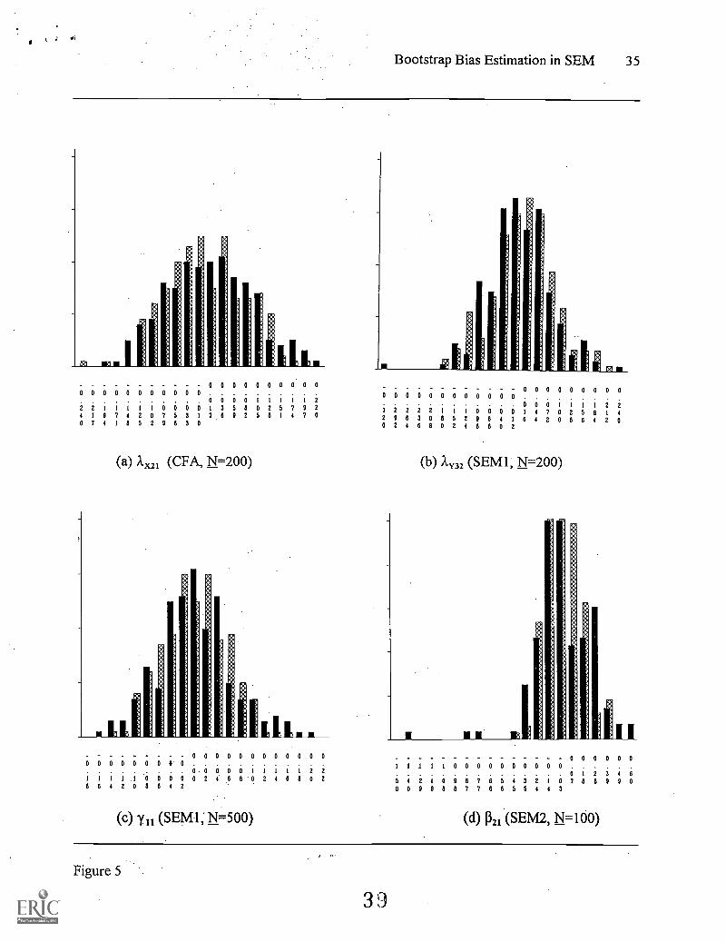
SEM loadings and Coefficients. Figure 5 present§ the distributional comparisons between

18


the bootstrap bias estimator and the Monte Carlo bias estimator for four SEM loadings and

coefficients [Axil (CFA Model, N=200), A., (SEM Model 1, N=200), y (SEM Model 1,

N=500), and p (SEM Model 2, N=100)]. It is seen that, for all the four coefficients, the

distributions of the bootstrap bias estimator and the Monte Carlo bias estimator are quite

comparable in terms of their range and shape, indicating that the bootstrap bias estimator is close

to the Monte Carlo bias estimator. Notice that, for these loadings and coefficients, there do not

exist any constraints caused by a theoretical ceiling or floor, as in the case for the fit indices. As a

result, bias estimator can be distributed in both directions (positive and negative) for both the

bootstrap and the Monte Carlo experiments. The similar distributions of the bootstrap and the

Monte Carlo bias estimators support the earlier discussion that the minuscule difference between

the two bias estimations observed in Table 2 is most probably inconsequential.


SEM variances and covariances. Figure 6 presents the distributional comparisons

between the bootstrap bias estimator and the Monte Carlo bias estimator for four SEM variances

and covariances [833(CFA Model, N=200), c (SEM Model 1, N=100), 4)2, (SEM Model 1,

N=500), and 813 (SEM Model 2, N=200)]. Similar to Figure 5, the distributions of the bootstrap

bias estimator and the Monte Carlo bias estimator are quite comparable in terms of their range

and shape, indicating that the bootstrap bias estimation is adequate. Unlike the SEM fit indices

discussed previously, for these (co)variances, there is no theoretical "ceiling" or "floor" which

constrains the bias in certain direction for Monte Carlo bias estimation. The similar distributions

of the bias estimators from the bootstrap and the Monte Carlo experiments suggest that the

19


difference between the bootstrap and the Monte Carlo bias estimations observed in Table 3 can be

considered small and inconsequential. As pointed out before, it is somewhat difficult to judge the

magnitude of bias for these variances and covariances because of their measurement scales.


SUMMARY AND CONCLUSIONS

This study examined the application of bootstrap method for bias estimation in the area of

SEM. Three correctly specified SEM models were used under four different sample size

conditions. Monte Carlo experiments were carried out to generate the criteria against which

bootstrap bias estimation could be judged. For the Monte Carlo experiments, 200 replications

were simulated within each cell condition, and the "true" bias of a statistic was obtained. For the

bootstrap experiments, one parent bootstrap sample was generated under each cell condition,

which served as the resampling space for bootstrapping within the cell. Two hundred bootstrap

samples were obtained from this parent sample through sampling with replacement. Bootstrapped

bias of a statistic was obtained and then compared with the bias of the statistic obtained from the

Monte Carlo experiments. Both the amount and direction of bias, and the distributions of the bias

estimator, from the bootstrap and Monte Carlo experiments were compared.

For SEM fit indices, bias estimation from the bootstrap and Monte Carlo experiments was

quite comparable for most of them in terms of both the direction and magnitude. It is noted that,

because true SEM models were simulated, bias was constrained in one direction in the Monte

Carlo experiments, but less so in the bootstrap experiments. Because of this, bootstrap bias

estimator has wider dispersion, and it was less skewed. It is hypothesized that if misspecified

2 0


SEM models were used in the study, the disparity between the bias estimator distributions from

these two kinds of experiments would be reduced, because in this situation, the less-than-perfect

population fit indices would function less as a constraint for the bias estimation in Monte Carlo

experiments.

For the SEM loadings and coefficients, the difference between bias estimations from the

bootstrap the Monte Carlo experiments was very small, although there did not appear to be a

consistent pattern. The distributions of the bias estimators from the two experiments were quite

similar both in terms of the shape and range, suggesting that the bootstrap bias estimation was

adequate because its bias estimator was comparable to that from the Monte Carlo experiments.

For the SEM variances/covariances, the picture is similar to that about SEM loadings and

coefficients. Because the measurement scales were quite different for these

variances/covariances, caution was warranted in interpreting the magnitude of the estimated bias

for these variances/covariances. The comparison of the distributions of the bias estimators from

the two experiments indicated that bootstrap bias estimation could be considered adequate

because of the similar distributions of the bias estimators from the two experiments.

To our knowledge, this is the first reported empirical study which provides direct

empirical evidence with regard to the adequacy of bootstrap bias estimation in SEM. It is our

hope that the findings from this study will make meaningful contribution to the SEM literature.

Because the study involved three SEM models which served as internal replication mechanism, we

are reasonably confident that the likelihood of chance discovery for the findings was small, and

the findings should be generalizable. Future studies may extend the current findings by examining

SEM models with some degree of misspecification, as discussed in this paper. In addition, data

non-normality may be another dimension which should be considered in future investigation.


REFERENCES

Bent ler, P. M. (1992). EQS structural equations program manual. Los Angeles, CA: BMDP

Statistical Software.

Bent ler, P. M. (1994). Forward. In B. M. Byrne, Structural Equation Modeling with EQS and

EQS/Windows. Thousand Oaks, CA: SAGE.

Bent ler, P. M., & Dudgeon, P. (1996). Covariance structure analysis: Statistical practice,

theory, and directions. Annual Review of Psychology, 47, 563-592.

Bagozzi, R. P., Fornell, C., & Larcker, D. F. (1981). Canonical correlation analysis as a

special case of structural relations model. Multivariate Behavioral Research, 16, 437-454.

Bollen, K. A. & Long, J. S. (1993). Introduction. In K. A. Bollen and J. S. Long (Eds.),

Testing structural equation models (pp. 1-9). Newbury Park, California: SAGE Publications.

Bollen, K. A., & Stine, R. (1990). Direct and indirect effects: Classical and bootstrap

estimates of variability. In C. C. Clogg (Ed.), Sociological methodology (pp. 115-140). Oxford:

Basil Blackwell.

Bollen, K. A., & Stine, R. (1993). Bootstrapping goodness-of-fit measures in structural

equation models. In K. A. Bollen & J. S. Long, (Eds.), Testing structural equation models (pp.

111-135). Newbury Park, CA: Sage.

Boomsma, A. (1982). The robustness of LISREL against small sample sizes in factor analysis

models. In K. G. Joreskog & H. Wold (Eds.), Systems under indirect observation: Causality,

structure, prediction (Part I) (pp. 149-175). Amsterdam: North-Holland.

Byrne, B. M. (1994). Structural equation modeling with EQS and EQS/Windows: Basic

concepts, applications, and programming. Newbury, California: SAGE Publications, Inc.

Calsyn, J. R., & Kenny, D. A. (1977). Self-concept of ability and perceived evaluation of

22


others: Cause or effect of academic achievement? Journal of Educational Psychology, 69, 136-

145.

Camstra, A., & Boomsma, A. (1992). Cross-validation in regression and covariance structure

analysis: An overview. Sociological Methods & Research, 21, 89-115.

Chatterjee, S. (1984). Variance estimation in factor analysis: An application of the bootstrap.

British Journal of Mathematical and Statistical Psychology, 37, 252-262.

Dalgleish, L. I. (1994). Discriminant analysis: Statistical inference using the jackknife and

bootstrap procedures. Psychological Bulletin, 116, 498-508.

Efron, B. (1979). Bootstrap methods: Another look at the jackknife. The Annals of Statistics,

7, 1-26.

Efron, B. (1985). Bootstrap confidence intervals for a class of parametric problems.

Biometrika, 72, 45-48.

Efron, B. (1995). Computers, bootstraps, and statistics. Invited address to American

Educational Research Association Annual-Meeting, Division D--Measurement and Research

Methodology. April, San Francisco, CA.

Fan, X. (1996). Structural equation modeling and canonical correlation analysis: What do

they have in common? Structural Equation Modeling: A Multidisciplinary Journal, 4, 64-78.

Fan, X., & Jacoby, W. R. (1995). BOOTSREG: A SAS matrix language program for

bootstrapping linear regression models. Educational and Psychological Measurement, 55, 764-

768.

Fan, X., & Mathews, T. A. (1994, April). Using bootstrap procedures to assess the issue of

predictive bias in college GPA prediction for ethnic groups. Paper presented at the annual

meeting of the American Educational Research Association, New Orleans. (ERIC Document

23


Reproduction Service #: ED 372 117).

Fan, X. & Wang, L. (1996). Comparability of jackknife and bootstrap results: An

investigation for a case of canonical analysis. Journal of Experimental Education, 64, 173-189.

Gall, M. D., Borg, W. R., & Gall, J. P. (1996). Educational research: An introduction (6th

ed.). White Plains, NY: Longman.

Gerbing, D. W., & Anderson, J. C. (1993). Monte Carlo evaluations of goodness-of-fit indices

for structural equation models. In K. A. Bollen & J. S. Long, (Eds.), Testing structural equation

models (pp. 40-65). Newbury Park, CA: SAGE Publications, Inc

Harris, D. J., & Kolen, M. J. (1989). Examining the stability of Angoffs delta item bias

statistic using bootstrap. Educational and Psychological Measurement, 49, 81-87.

Hu, L., Bentler, P. M., & Kano, Y. (1992). Can test statistics in covariance structure analysis

be trusted? Psychological Bulletin, 112, 351-362.

Ichikawa, M., & Konishi, S. (1995). Application of the bootstrap methods in factor analysis.

Psychometrika, 60, 77-93.

Joreskog, K. G. & S6rbom, D. (1989). LISREL 7: A Guide to the Program and applications,

2nd Edition. Chicago, IL: SPSS Inc.

Kaiser, H.F., & Dickman, K. (1962). Sample and population score matrices and sample

correlation matrices from an arbitrary population correlation matrix. Psychometrika, 27, 179-182.

Kotz, S., & Johnson, N. L. (1992). Breakthroughs in statistics: Volumes 1 and 2. New

York: Springer-Verlag.

Lambert, Z. V., Wildt, A. R., & Durand, R. M. (1991). Approximating confidence intervals

for factor loadings. Multivariate Behavioral Research, 26, 421-434.

Loehlin, J. C. (1992). Latent variable models: An introduction to factor, path, and structural

2 4


analysis. Hillsdale, New Jersey: Lawrence Erlbaum Associates, Publishers.

Mac Callum, R. C., Roznowski, M., & Necowitz, L. B. (1992). Model modifications in

covariance structure analysis: The problem of capitalization on chance. Psychological Bulletin,

111, 490-504.

Marsh, H. W., Balla, J. R., & McDonald, R. P. (1988). Goodness-of-fit indexes in

confirmatory factor analysis: The effect of sample size. Psychological Bulletin, 103, 391-410.

Rasmussen, J. L. (1987). Estimating the correlation coefficients: Bootstrap and parametric

approaches. Psychological Bulletin, 101, 136-139.

SAS Institute, Inc. (1990). SAS/STAT user's guide, version 6 (vol. 1, 4th ed.). Cary, NC:

SAS Institute Inc.

Stine, R. A. (1989). An introduction to bootstrap methods: Examples and ideas. Sociological

Methods and Research, 8, 243-291.

Tanaka, J. S. (1987). "How big is big?": Sample size and goodness-of-fit in structural

equation models with latent variables. Child Development, 58, 134-146.

Thompson, B. (1988). Program FACSTRAP: A program that computes bootstrap estimates

of factor structure. Educational and Psychological Measurement, 48, 681-686.

Thompson, B. (1993). The use of statistical significance tests in research: Bootstrap and other

alternatives. The Journal of Experimental Education, 61, 361-377.

Wheaton, D. E., Muthén, B., Alwin, D. F., & Summers, G. F. (1977). Assessing reliability

and stability in panel models. In D. R. Heise (Ed.), Sociological methodology 1977 (pp. 84-136).

San Francisco: Jossey Bass.

Yung, Y., & Bentler, P. M. (1996). Bootstrapping techniques in analysis of mean and

covariance structures. In G. A. Marcoulides & R. E. Schumacker (Eds.), Advanced structural

25


equation modeling: Issues and techniques (pp. 195-226). Mahwah, New Jersey: Lawrence

Erlbaum.

26

Boo

tstr

ap B

ias

Est

imat

ion

in S

EM

26

Tab

le 1

Com

pari

son

of B

oots

trap

(B

trap

) B

ias

Est

imat

ion

and

"Tru

e" B

ias

for

SEM

Fit

Indi

ces

MO

DE

L'

NSO

UR

CE

x2R

MR

bG

FIA

GFI

CFI

CE

NT

RA

NN

FIN

FIR

HO

1A

2P

GFI

PAR

MS

CFA

1 00

Btr

ap8.

031

.033

-.02

2-.

079

-.02

5-.

037

-.06

4-.

024

-.05

9-.

025

-.00

9-.

009

"Tru

e"8.

171

.147

-.02

6-.

091

-.00

8-.

014

-.02

0-.

022

-.05

5-.

008

-.01

0-.

009

200

Btr

ap6.

779

.036

-.01

1-.

037

-.01

0-.

017

-.02

4-.

009

-.02

3-.

009

-.00

4-.

004

"Tru

e"8.

508

.109

-.01

4-.

048

-.00

4-.

009

-.01

3-.

012

-.03

0-.

005

-.00

6-.

005

500

Btr

ap7.

877

.022

-.00

5-.

018

-.00

4-.

008

-.01

1-.

004

-.01

1-.

004

-.00

2-.

002

"Tru

e"7.

869

.064

-.00

5-.

018

-.00

1-.

005

-.00

7-.

004

-.01

1-.

003

-.00

2-.

002

1000

Btr

ap6.

913

.015

-.00

2-.

008

-.00

2-.

003

-.00

5-.

002

-.00

5-.

002

-.00

1-.

001

"Tru

e"8.

330

.047

-.00

3-.

010

-.00

1-.

004

-.00

6-.

002

-.00

6-.

002

-.00

1-.

001

SEM

I10

0B

trap

47.8

081.

713

-.05

4-.

090

-.05

6-.

193

-.07

9-.

049

-.06

9-.

055

-.03

9-.

035

"Tru

e"45

.231

4.74

5-.

074

-.12

3-.

007

-.03

8-.

012

-.05

3-.

074

-.00

9-.

052

-.03

7

200

Btr

ap48

.117

1.28

9-.

034

-.05

7-.

026

-.11

4-.

040

-.02

6-.

037

-.02

8-.

024

-.01

9

"Tru

e"48

.767

3.42

9-.

038

-.06

4-.

003

-.02

8-.

009

-.02

6-.

037

-.00

6-.

027

-.01

9

500

Btr

ap49

.339

.860

-.01

5-.

025

-.01

1-.

047

-.01

6-.

011

-.01

6-.

011

-.01

1-.

008

"Tru

e"48

.473

2.11

9-.

016

-.02

6-.

001

-.02

5-.

008

-.01

1-.

015

-.00

6-.

011

-.00

8

1000

Btr

ap47

.430

.569

-.00

8-.

013

-.00

5-.

023

-.00

7-.

005

-.00

7-.

005

-.00

5-.

004

"Tru

e"46

.771

1.50

9-.

008

-.01

3-.

000

-.02

4-.

007

-.00

5-.

007

-.00

5-.

005

-.00

4

SEM

210

0B

trap

2.64

0..0

71-.

007

-.03

7-.

012

-.01

2-.

043

-.01

0-.

036

-.01

1-.

002

-.00

3"T

rue"

4.13

0.1

78-.

013

-.07

0-.

005

-.00

3-.

008

-.01

7-.

063

-.00

2-.

004

-.00

4

200

Btr

ap4.

095

.031

-.00

6-.

034

-.01

0-.

010

-.03

4-.

009

-.03

2-.

009

-.00

2-.

002

"Tru

e"3.

994

.120

-.00

7-.

034

-.00

2-.

002

-.00

6-.

008

-.03

1-.

002

-.00

2-.

002

500

Btr

ap3.

143

.025

-.00

2-.

011

-.00

2-.

003

-.01

0-.

003

-.01

0-.

003

-.00

1-.

001

"Tru

e"4.

024

.076

-.00

3-.

014

-.00

1-.

002

-.00

7-.

003

-.01

3-.

002

-.00

1-.

001

1000

Btr

ap3.

838

.017

-.00

1-

007

-.00

2-.

002

-.00

6-.

002

-.00

6-.

002

-.00

0-.

000

"Tru

e"4.

332

.056

-.00

I-.

008

-.00

1-.

002

-.00

7-.

002

-.00

7-.

002

-.00

0-.

001

a C

FA: c

onfi

rmat

ory

fact

or a

naly

sis

mod

el; S

EM

I: s

truc

tura

l equ

atio

n m

odel

1; S

EM

2: s

truc

tura

l equ

atio

n m

odel

2.

b R

MR

: Roo

t Mea

n-Sq

uare

Res

idua

l; G

FI: G

oodn

ess-

of-f

it in

dex;

AG

FI: A

djus

ted

good

ness

-of-

fit i

ndex

; CFI

: com

para

tive

fit i

ndex

; CE

NT

RA

:M

cDon

ald'

s ce

ntra

lity

inde

x; N

NFI

: Ben

tler-

Bon

nett'

s no

n-no

rmed

fit

inde

x; N

FI: B

entle

r-B

onne

tt's

norm

ed f

it in

dex;

RH

O!:

Bol

len'

s R

hol;

Bol

len'

s de

lta2

(inc

rem

enta

l fit)

inde

x; P

GFI

: Jam

es e

t al.'

s pa

rsim

onio

us g

oodn

ess-

of-f

it in

dex;

PA

RM

S: M

ulai

k et

al.'

s pa

rsim

onio

us f

it in

dex.

2728

Boo

tstr

ap B

ias

Est

imat

ion

in S

EM

27

Tab

le 2

Com

pari

son

of B

oots

trap

(B

trap

) B

ias

Est

imat

ion

with

"T

rue"

Bia

s fo

r SE

M L

oadi

ngs

and

Coe

ffic

ient

s

Mod

elN

Sour

ceA

xil

Ax2

1A

xmA

x41

452

XX

62

CFA

100

200

Btr

ap-.

0040

"Tru

e".0

004

Btr

ap-.

0030

"Tru

e".0

004

.000

2-.

0033

.008

4.0

011

.019

1.0

027

.006

2.0

021

-.00

09-.

0011

.006

0-.

0028

-.00

21-.

0003

-.00

32-.

0001

-.00

08.0

039

-.00

03.0

040

500

Btr

ap-.

0002

-.00

55.0

000

-.00

13-.

0005

-.00

26"T

rue"

-.0

001

-.00

41.0

036

.001

0-.

0004

-.00

13

1000

Btr

ap-.

0005

.000

4-.

0027

-.00

17-.

0010

-.00

02"T

rue"

.000

1.0

008

-.00

41-.

0021

-.00

00-.

0006

Mod

elN

Sour

ceA

xil

421

422

431

432

442

411

421

422

431

432

)Y42

Yil

Y22

SEM

I10

0B

trap

.003

7-.

0046

-.00

82.0

000

.001

5.0

097

-.02

31-.

0287

-.01

01-.

0308

-.00

80.0

006

.027

1.0

086

"Tru

e" -

.006

6.0

020

.004

0-.

0006

.008

2.0

012

.000

3-.

0048

.006

3.0

009

.008

6.0

579

-.00

02-.

0039

200

Btr

ap.0

012

.003

0.0

046

.009

3-.

0018

.008

3-.

0025

.000

8-.

0005

.004

7-.

0010

-.00

45.0

015

.004

4"T

rue"

.004

2-.

0032

.001

5.0

000

-.00

03-.

0059

.015

2.0

052

0030

.000

5.0

070

.045

3.0

032

-.00

18

500

Btr

ap.0

001

-.00

19-.

0017

-.00

37.0

022

.004

4-.

0014

-.00

35-.

0012

-.00

01-.

0021

.000

3.0

021

.001

9"T

rue"

.001

8-.

0019

.000

4-.

0012

.001

4.0

009

.007

1.0

001

-.00

02.0

029

-.00

54.0

460

-.00

13.0

031

1000

Btr

ap.0

016

.002

4.0

011

-.00

01.0

001

.001

0-.

0041

.000

6.0

018

-.00

17.0

011

-.00

17.0

041

.000

6"T

rue"

.002

6-.

0008

.001

3.0

012

.000

2.0

002

-.00

07.0

020

-.00

43-.

0003

-.00

21.0

484

.002

2.0

008

Mod

elN

Sour

ce41

142

144

2ii

Y2

P

SEM

210

0B

trap

.106

4.0

364

.097

7-.

1007

-.15

20-.

0240

"Tru

e".0

164

-.01

41.0

055

-.04

41-.

0274

-.01

18

200

Btr

ap-.

0199

-.04

69-.

0304

-.01

66.0

210

.007

0"T

rue"

.010

9.0

002

-.00

29-.

0023

.001

6.0

013

500

Btr

ap.0

031

.003

5.0

011

-.00

70-.

0013

-.00

11"T

rue"

-.0

026

.012

7.0

085

.008

3-.

0005

-.00

15

1000

Btr

ap.0

012

.000

6.0

019

-.00

08-.

0070

-.00

56"T

rue"

.002

2-.

0033

-.00

32-.

0039

-.00

27.0

005

2930

Boo

tstr

ap B

ias

Est

imat

ion

Tab

le 3

Com

pari

son

of B

oots

trap

(B

trap

) B

ias

Est

imat

ion

with

"T

rue"

Bia

s fo

r SE

M V

aria

nces

and

Cov

aria

nces

in S

EM

Mod

el N

Sour

ceoi

l82

283

384

485

586

64)

1141

2243

121

CFA

100

Btr

ap.0

48-.

051

-.12

0-.

044

.004

-.03

7-.

007

-.07

6-.

007

"Tru

e"-.

067

-.01

9-.

016

-.00

4-.

032

-.03

8.1

42.0

22.0

62

200

Btr

ap.0

18-.

047

-.02

4-.

049

-.03

3-.

012

-.09

7-.

018

-.06

8"T

rue"

-.01

3.0

29-.

020

.019

.001

-.01

1-.

006

-.09

8-.

052

500

Btr

ap-.

011

-.01

4.0

04-.

017

-.02

4-.

012

-.01

6.0

08.0

00"T

rue"

.007

-.00

1.0

06-.

015

-.00

8-.

002

.001

.022

.001

1000

Btr

ap-.

017

-.01

7-.

017

-.01

2-.

005

-.00

1-.

002

-.00

6-.

001

"Tru

e".0

03.0

03.0

04-.

001

-.00

6.0

01-.

004

-.00

0-.

018

Mod

el N

....o

urce

On

822

833

844

855

866

C11

C22

C33

C44

C55

C66

4)11

14)2

24)

21*1

1*2

2

28

SEM

I10

0B

trap

-.40

7-.

528

-.28

9-.

517

-.76

1-1

.176

-.94

3-1

.236

-.65

2-.

127

-.65

9-.

996

-2.5

13-1

.418

-1.1

38.9

50.7

47

"Tru

e" -

1.06

9 -1

.205

-.69

4.3

66-.

207

-.31

9.4

44-.

471

-1.2

95-.

714

-.40

8-.

898

2.49

3-.

160

.056

.020

.029

200

Btr

ap-.

792

-.28

7-1

.266

-.36

0-.

191

-1.2

05.1

84-.

971

-.55

1-.

064

-.38

6-.

106

.217

-1.3

56.3

66.8

03-.

I 1

3

"Tru

e"-.

453

-.48

9-.

543

-.38

1-.

095

.024

-.44

4-.

236

-.61

3-.

266

-.21

8-.

046

-.14

7.9

93-.

706

-.78

9.0

23

500

Btr

ap-.

203

-.17

1.0

09-.

074

.060

-.17

4-.

038

-.40

1-.

261

-.17

1.0

09-.

350

-.38

2-.

690

-.27

3.4

98.0

77

"Tru

e".3

91-.

230

-.45

5-.

012

-.02

4-.

146

-.26

6-.

006

.021

.129

-.20

4.1

79.4

68.0

90.3

91-.

489

.028

1000

Btr

ap-.

119

-.15

5-.

322

-.02

7-.

152

-.07

0-.

038

-.01

8-.

087

.169

-.08

2-.

691

.065

-.23

3.3

99.0

65.0

44

"Tru

e"-.

336

-.04

0-.

258

.062

-.09

2-.

122

-.01

1.0

34-.

092

-.34

3-.

340

.030

-.60

1.4

94.0

33.0

71.1

59

Mod

el N

Sour

ce01

182

2el

lC

22C

33C

444)

11*1

1*2

2C

13C

24

SEM

210

0B

trap

.355

-.21

0-.

154

-.23

8.3

15-.

622

-.41

3-.

355

-.76

0.0

54-.

215

"Tru

e".0

32-.

129

-.18

9-.

005

-.17

8.0

17.0

15.0

72-.

083

-.01

0-.

032

200

Btr

ap-.

520

.059

-.41

3.3

41-.

418

193

.506

.212

.138

-.27

1.2

52"T

rue"

-.03

3-.

039

-.10

4.0

69-.

166

.024

.083

.025

-.00

3-.

139

.081

500

Btr

ap-.

026

-.04

2.0

30-.

054

-.02

8-.

029

.013

.002

-.03

9.0

41-.

036

"Tru

e"-.

071

.006

.069

-.07

4.1

06-.

082

.092

-.02

9-.

019

.066

-.04

7

1000

Btr

ap-.

053

-.00

4-.

045

-.02

9-.

028

.007

.050

-.00

6-.

048

-.00

4-.

006

"Tru

e"-.

010

.003

.-.

054

.020

-.02

4.0

03-.

005

.012

-.00

2-.

022

-.00

3

3132

Table 4

Bootstrap Bias

Number of Samples with Improper Solutions

Estimation in SEM

Sample N Experiment

SEM Models

CFA SEMI SEM2

100 Bootstrap 15 17 41

Monte Carlo 1 2 22


Monte Carlo 0 0 6

500 Bootstrap 0 0 3

Monte Carlo 0 0 0


Monte Carlo 0 0 0

29


Figure Captions

Figure 1. Confirmatory Factor Analysis Model and Model Specifications

Figure 2. Structural Equation Model 1 and Model Specifications

Figure 3. Structural Equation Model 2 and Model Specifications

Figure 4. Comparison of Bias Estimator Distributions for Four SEM Fit Indices (Black

Bars: Bootstrap; Shaded Bars: Monte Carlo)

Figure 5. Comparison of Bias Estimator Distributions for Four SEM Loadings and

Coefficients (Black Bars: Bootstrap; Shaded Bars: Monte Carlo)

Figure 6. Comparison of Bias Estimator Distributions for Four SEM Variances/Covariances

(Black Bars: Bootstrap; Shaded Bars: Monte Carlo)

3 4


A,

1.00 0.00

0.85 0.00

0.80 0.00

0.70 0.00

0.00 1.00

0.00 0.75

0, (Diagonal) =

1.25

2.25

2.50

2.50

1.50

1.10

(1) =4.00

5.00

X 3

5.00 I

9.00

Figure 1

35


0.95 0.00 0.90 0.00

0.20 0.50 0.25 0.65

0.25 0.85 0.35 0.70Ax = Ay =

0.00 1.20 0.00 0.95

0.00 1.00 0.00 1.00

1.00 0.00 1.00 0.00

0.90 0.00 Ir=0.00 0.80

0.00 0.00 IB

0.00 0.00

105.00 50.00 I

50.00 115.00

18.00 0.00ljr =

I

0.00 6.00

30.00 25.00

30.00 40.00

40.00 50.000, (Diagonal) = 0c (Diagonal) =

45.00 40.00

20.00 20.00

50.00 70.00

1.00 f: Fixed to be 1

Figure 2

36


0, =

=1.00 I

0.50

-0.60 Ir-0.25

B=F 0.00 0.00 I

0.60 0.00

3.00 0.00 I0.00 2.50

Ay =

1.00 0.00

0.95 0.00

0.00 1.00

0.00 0.90

(1) = [ 7.00 ]

0, =

=

4.75

0.00

1.60

0.00

5.00

0.00

2.50

0.00

0.30

0.00

4.00

4.50

0.00 3.00

Y1 Y2 Y3 Y4

xl X21.00f: Fixed to be 1.00

Figure 3


..i it 'fill,.0 0 0 0 0 0 0 0 0 0 0 0 0 0

0 0 0 0 0 0 0

0 0 0 0 0 0 0

0 0 0 0 0 O. 0 0 0 0 0 0 0 0 0 0 I I 2 2 3

5 5 4 4 3 3 2 2 I I I 0 0 1 / 2 6 I 5 0

0 5 I 6 2 1 3 8 4 9 5 0 6 I 0 5 0 5 0 5 0

0 5 0 5 0 5 0 0 5 0 5 0 5

(a) GFI (SEM2, N=100)

-7 -5 -9 -1 1 . 3 5. 7 9 11 19 15 17 19 21 23 25 27 29 31 93

0 0 0 00 0 0 0 0 0 0 0 0 0 0 0 0 0 0 0 0

6 6 0 60 0 0 0 0 0 0 0 0 0 0 0 0 0 0 0 0 0 0 0 1

5 4 4 4 3 3 3 2 2 2 2 1 1 1 0 0 0 1 4 7 00 7 4 1 .8 5 2 9 6 3 0 7 4 1 8 5 2

(b) NFI (CFA, N=200)

...11111116,111- - 0 0 0 0 1 1 1 2 2 2 2 3 3 3 4 4 4 50 0 0

. 0 3 6 9 2 5 8 1 3 6 9 2 5 8 1 4 7 08, 5 2 7 6 5 4 3 2 1 0 9 8 7 6 5 4 3 2 1 00 1 2

(c) Xi (CFA, N=200) (d) RMR (SEMI, N=100)

Figure 4

38


31.11i1111111ILLE0 0 0 0 0 0 0 0. 0 0

0 0 0 0 0 0 0 0 00 0 0 0 0 0 0 0 0 0 0 0 0 0 0 0 0 0 0 0 0 0 00 0 0 0 I I I 1 I 2

0 0 0 1 1 1 1 2 22 2 I I I I 0 0 0 0 1 3 5 8 0 2 5 7 9 2 32222 1110 000 I 4 7 0 2 5 8 I 44 1 9 7 4 2 0 7 5 3 1 3 6 9 2 5 8 1 4 7 0 2 9 6 3 0 8 5 2 9 6 4 1 6 4 2 0 8 6 4 2 00 7 4 1 8 5 2 9 6 3 0 0 2 4 6 8 0 2 4 6 8 0 2

(a) x2 (CFA, N=200) (b) y3 2 (SEM1, N=200)

Nil0 0 0 0 0 0 0 0 0 0 0 0 0 0 0 0 0 0

0 0 0 0 0 0 0 0 0 I I .1 1 1 0 0 0 0 0 0 0 0 0 0000001111122 0 1 2 3 4 61 1 1 1 .1 0 0 0 0 0 -2 f 6 8 -0 2 4 6 8 0 2 5 4 2 1 0 9 8 7 1 3 5 4 3 2 1 0 7 8 8 9 9 08 6 4 2 0 8 6 4 2 0 0 9 9 8 8 7 7 6 6 5 5 4 4 3

(c) y I (SEMI; N=500) (d) p21 (SEM2, N=100)

Figure 5

3 9

4 c


000000000

65

000000000001012344567890765432110754219865320023568902

135791111122111197531 13579207531 0123454321 56789009876

(a) 833 (CFA, N=200) (b) E (SEM1, N=100)

111111111 i013579111111111197531 0246886420 08642002468 8642002468

(c) 43021 (SEM1, N=500)

3 2'22211110000 00001111136803580 75208530.8631260482600 628406284062

(d) en (SEM2, N=200)

Figure 6

U.S. Department of EducationOffice of Educational Research and Improvement (OERI)

National Library of Education (NLE)Educational Resources Information Center (ERIC)

REPRODUCTION RELEASE(Specific Document)

I. DOCUMENT IDENTIFICATION:

RICTM028952

Title: Bootstrap Estimation of Sample Statistic Bias in Structural Equation Modeling

AUthol(s): Xitao Fan Bruce Thompson

Corporate Source:

Utah State University

Publication Date:

April 13, 1998

II. REPRODUCTION RELEASE:

In order to disseminate as widely as possible timely and significant materials of interest to the educational community, documents announced in themonthly abstract journal of the ERIC system, Resources in Education (RIE), are usually made available to users in microfiche, reproduced paper copy,and electronic media, and sold through the ERIC Document Reproduction Service (EDRS). Credit is given to the source of each document, and, Ifreproduction release is granted, one of the following notices is affixed to the document.

If permission is granted to reproduce and disseminate the identified document, please CHECK ONE of the following three options and sign at the bottomof the page.

The sample Wicker shown below will beaffixed to all Level 1 documents

1

PERMISSION TO REPRODUCE ANDDISSEMINATE THIS MATERIAL HAS

BEEN GRANTED BY

5,6

\e


Level 1

Check here for Level 1 release, permitting reproductionand dissemination in microfiche or other ERIC ardaval

media (e.g., electronic) and paper copy.

Sign

please

The sample sticker shown below will beaffixed to all Level 2A documents

PERMISSION TO REPRODUCE ANDDISSEMINATE THIS MATERIAL IN

MICROFICHE, AND IN ELECTRONIC MEDIAFOR ERIC COLLECTION SUBSCRIBERS ONLY,

HAS BEEN GRANTED BY

2A

45cTO THE EDUCATIONAL RESOURCES

INFORMATION CENTER (ERIC)

Level 2A

Check here for Level 2A release, permitting reproductionand dissemination In microfiche and in electronic media

for ERIC archival collection subsaibers only

The sample sticker shown below will beaffixed to all Level 2B documents

PERMISSION TO REPRODUCE ANDDISSEMINATE THIS MATERIAL IN

MICROFICHE ONLY HAS BEEN GRANTED BY

2B


Uwel2B

Check here for Level 28 release, pennlftitigreproduction end dissemination in microfiche onty

Documents will be processed as Indicated provided reproduction quality permits.If permission to reproduce I. granted, but no box Is checked, documents will be processed at Level 1.

I hereby grant to the Educational Resources Information Center (ERIC) nonexclusive permission to reproduce and disseminate this documentas indicated above. Reproductidn from the ERIC microfiche or electronic media by persons other than ERIC employees and its systemcontractors requires permission from the copyright holder. Exception Is made for non-profit reproduction by libraries and other service agenciesto satisfy Information needs of educators In response to discrete Inquiries.

&matte: Printed Name/Position/Title:

Xitao Fan Assistant ProfessorOrgwilzation/Address:

Dept. of PsychologyUtah State University, Logan, UT 84322-2810

Telephone:(435)797-1451

E-Mail Address:[email protected].

FAX(435)797-1448

Dlinril 28, 1998

(over)

ERIC Clearinghouse on Assessment and Evaluation

March 20, 1998

Dear AERA Presenter,

Congratulations on being a presenter at AERA1. The ERIC Clearinghouse on Assessment and Evaluationinvites you to contribute to the ERIC database by providing us with a printed copy of your presentation.

Abstracts of papers accepted by ERIC appear in Resources in Education (RIE) and are announced to over5,000 organizations. The inclusion of your work makes it readily available to other researchers, provides apermanent archive, and enhances the quality of RIE. Abstracts of your contribution will be accessiblethrough the printed and electronic versions of RIE. The paper will be available through the microfichecollections that are housed at libraries around the world and through the ERIC Document ReproductionService.

University of Maryland1129 Shriver Laboratory

College Park, MD 20742-5701

Tel: (800) 464-3742(301) 405-7449

FAX: (301) [email protected]

http://ericae.net

We are gathering all the papers from the AERA Conference. We will route your paper to the appropriateclearinghouse. You will be notified if your paper meets ERIC's criteria for inclusion in RIE: contributionto education, timeliness, relevance, methodology, effectiveness of presentation, and reproduction quality.You can track our processing of your paper at http://ericae.net.

Please sign the Reproduction Release Form on the back of this letter and include it with two copies of yourpaper. The Release Form gives ERIC permission to make and distribute copies of your paper. It does notpreclude you from publishing your work. You can drop off the copies of your paper and ReproductionRelease Form at the ERIC booth (424) or mail to our attention at the address below. Please feel free tocopy the form for future or additional submissions.

Mail to: AERA 1998/ERIC AcquisitionsUniversity of Maryland1129 Shriver LaboratoryCollege Park, MD 20742

This year ERIC/AE is maldrig a Searchable Conference Program available on the AERA web page(http://aera.net). Check it out!

Lawrence M. Rudner, Ph.D.Director, ERIC/AE

-'If you are an AERA chair or discussant, please save this form for future use.

The Catholic University of America