P, NP and NPC

Course notes for Combinatorial Search

Spring 2007

Peter Bro Miltersen

April 3, 2007

Version 3.1

1 Decision problems and languages

In this note we shall develop the theory of NP-completeness. The theorywill enable us to show that concrete search and optimization problems arethe “least likely” among all “simple” search and optimization problems tohave polynomial time algorithms (a notion which will also be made rigorousin this note).

Our first task is to make a restriction of the problems we are going to look at:We shall focus on decision problems, i.e., problems for which the output tobe computed on a given input (i.e., problem instance) should be either “yes”or “no”. Furthermore, we are going to look only on problems where eachinstance is given by a string over {0, 1}. Such a problem can be described asa language, i.e., a subset L of {0, 1}∗ with the members of L being the inputsfor which the answer to be computed is “yes” and the non-members beingthe inputs for which the answer to be computed is “no”.

The following comments and clarifications should convince us that this seem-ingly restrictive framework is in fact quite general.

First let us discuss the restriction of inputs to being strings over {0, 1}. Thefact that the alphabet is {0, 1} and not some other alphabet is inconse-quential: If we have a problem with inputs that we prefer to describe overa different (and most likely bigger) alphabet Σ, we may encode each sym-bol σ ∈ Σ as a string over {0, 1} of length dlog2 |Σ|e and then represent astring over Σ by the concatenation of the encodings of its symbols. Indeed,this is the way bigger alphabets such as ASCII and UNICODE are actu-ally represented on real computers. Thus, we are really merely restrictingour inputs to be strings over some finite alphabet. On the other hand, weare ruling out problems where the input is, say, a vector of arbitrary realnumbers, and thus it seems that we are ruling out some of the problems wealready looked at, such as network flow problems and linear programming.But, we should remember that strings over {0, 1} are in reality the onlyobjects that are actually present in a digital computer, its memory imagebeing itself such a string! So even if we did not make the restriction in ourtheory, we would have to make it in practice anyway. For instance, eventhough it may be a useful abstraction to view, say, the simplex algorithmas operating on arbitrary real numbers, we have to make a restriction onthe actual set of numbers used when we implement it. A “dirty” but usefulsuch restricted set of numbers would be the set of floating point numbers ofsome precision, while a cleaner choice would be the set of rational numbers(which will be our choice when we look at problems such a linear program-

2

ming in this note). In either case, we may represent the restricted set ofnumbers as strings over a finite alphabet. Also, combinatorial objects suchas graphs (used, for instance, to specify a flow networks) are easily repre-sentable as strings - and must be, as we can give them as inputs to realsoftware. So, demanding a representation of problem instances as strings isnot a real limitation. Which representation to use usually does not mattermuch - but sometimes it does. This point will be discussed more in the nextsection, where we define the complexity class P. One standard concrete rep-resentation which we will introduce now for convenience is the pairing func-tion 〈·, ·〉: If x = x1x2 . . . xn and y = y1y2 . . . ym are strings over {0, 1}, welet 〈x, y〉 denote the string x10x20 . . . xn−10xn011y10y20 . . . ym−10ym0. Notethat 〈x, y〉 is also a string over {0, 1} and that x and y may be recon-structed from 〈x, y〉. We generalize the notation to tuples and lists, e.g.,if x = x1x2 . . . xn, y = y1y2 . . . ym and z = z1z2 . . . zl we let 〈x, y, z〉 denotethe string x10x20 . . . xn−10xn011y10y20 . . . ym−10ym011z10z20 . . . zl−10zl0 andsimilar for 4-tuples, 5-tuples, etc. We shall reserve the 〈·, ·〉 notation for pair-ing functions in this note and not use it to denote inner products. Instead,we write the inner product of vectors c and x as cTx. Also, for a naturalnumber n, we let b(n) ∈ {0, 1}∗ denote its binary notation.

Given a particular choice on how to represent inputs by strings, a givenstring may represent no legal input. For instance, if we represent directedgraphs by square adjacency matrices and represent the adjacency matricesas {0, 1}-strings by concatenating their rows, only inputs of length m =n2 for some integer n actually represent graphs. We may want to thinkof an input of non-square length m as being neither a “yes”-instance nora “no”-instance, but rather being a malformed instance. However whenformalizing decision problems as languages we do demand every string to beeither a “yes”-instance or a “no”-instance, and we shall simply categorize themalformed instances as “no”-instances. Lumping the malformed instanceswith the “no”-instances shall work just fine in the theory we shall develop.

The restriction to decision problems or languages, i.e., the restriction tooutputs being “yes” or “no” is also less serious than it may first appear.For instance, suppose we really want to have arbitrary Boolean strings asoutputs (and as for the inputs, Boolean strings are in reality the only objectsdigital computers may give as outputs) and want to compute a functionf : {0, 1}∗ → {0, 1}∗. We can then represent f by the decision problem Lf

with

Lf = {〈x, b(j), y〉|x ∈ {0, 1}∗, j ∈ N, y ∈ {0, 1}, f(x)j = y}.

3

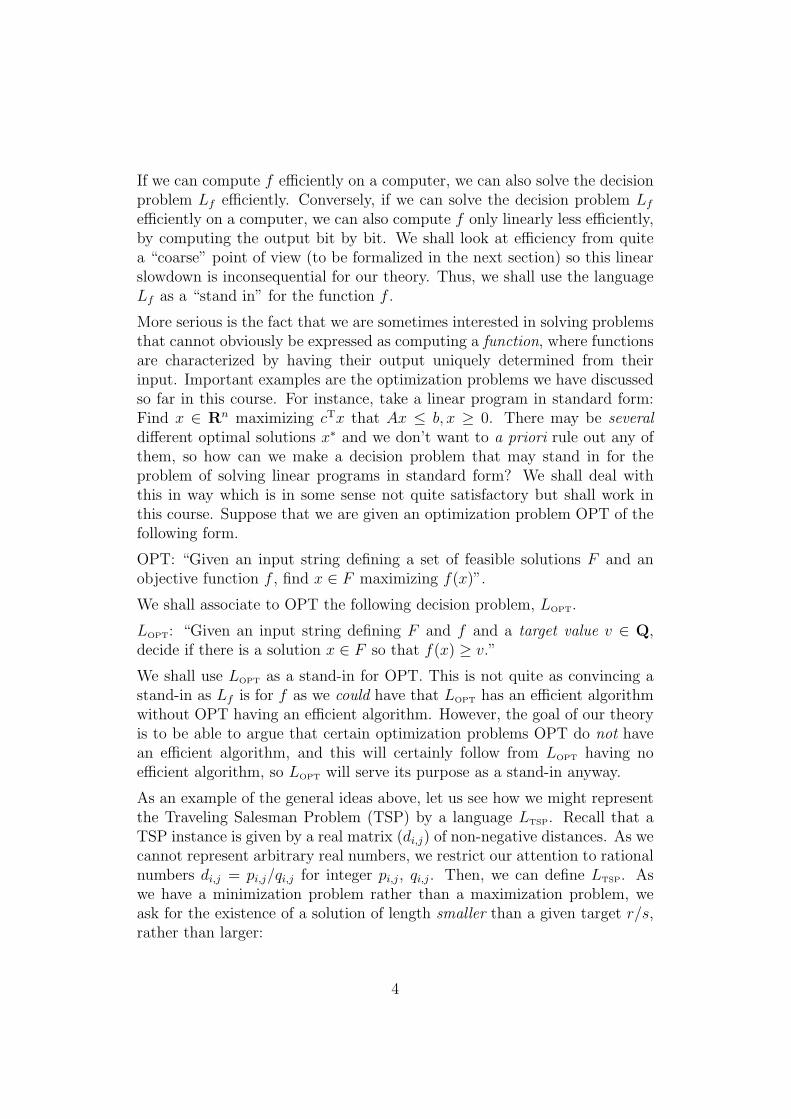
If we can compute f efficiently on a computer, we can also solve the decisionproblem Lf efficiently. Conversely, if we can solve the decision problem Lf

efficiently on a computer, we can also compute f only linearly less efficiently,by computing the output bit by bit. We shall look at efficiency from quitea “coarse” point of view (to be formalized in the next section) so this linearslowdown is inconsequential for our theory. Thus, we shall use the languageLf as a “stand in” for the function f .

More serious is the fact that we are sometimes interested in solving problemsthat cannot obviously be expressed as computing a function, where functionsare characterized by having their output uniquely determined from theirinput. Important examples are the optimization problems we have discussedso far in this course. For instance, take a linear program in standard form:Find x ∈ Rn maximizing cTx that Ax ≤ b, x ≥ 0. There may be severaldifferent optimal solutions x∗ and we don’t want to a priori rule out any ofthem, so how can we make a decision problem that may stand in for theproblem of solving linear programs in standard form? We shall deal withthis in way which is in some sense not quite satisfactory but shall work inthis course. Suppose that we are given an optimization problem OPT of thefollowing form.

OPT: “Given an input string defining a set of feasible solutions F and anobjective function f , find x ∈ F maximizing f(x)”.

We shall associate to OPT the following decision problem, LOPT.

LOPT: “Given an input string defining F and f and a target value v ∈ Q,decide if there is a solution x ∈ F so that f(x) ≥ v.”

We shall use LOPT as a stand-in for OPT. This is not quite as convincing astand-in as Lf is for f as we could have that LOPT has an efficient algorithmwithout OPT having an efficient algorithm. However, the goal of our theoryis to be able to argue that certain optimization problems OPT do not havean efficient algorithm, and this will certainly follow from LOPT having noefficient algorithm, so LOPT will serve its purpose as a stand-in anyway.

As an example of the general ideas above, let us see how we might representthe Traveling Salesman Problem (TSP) by a language LTSP. Recall that aTSP instance is given by a real matrix (di,j) of non-negative distances. As wecannot represent arbitrary real numbers, we restrict our attention to rationalnumbers di,j = pi,j/qi,j for integer pi,j, qi,j. Then, we can define LTSP. Aswe have a minimization problem rather than a maximization problem, weask for the existence of a solution of length smaller than a given target r/s,rather than larger:

4

LTSP = {〈 b(p0,0), b(q0,0), b(p0,1), b(q0,1), . . . , b(p0,n−1), b(q0,n−1),b(p1,0), b(q1,0), b(p1,1), b(q1,1), . . . , b(p1,n−1), b(q1,n−1),. . .b(pn−1,0), b(qn−1,0), b(pn−1,1), b(qn−1,1) . . . , b(pn−1,n−1), b(qn−1,n−1),b(r), b(s) 〉|∃ permutation π on {0, 1, . . . , n− 1} :

∑n−1i=0

pπ(i),π((i+1) mod )

qπ(i),π((i+1) mod n)≤ r

s}

2 Turing machines and P

The Turing machine model is a primitive, yet general model of computation.We shall use it in in this section to make precise and completely rigorous thenotion of a polynomial time algorithm.

A Turing machine consists of

1. A (potentially infinite) bi-directional tape divided into cells each ofwhich is inscribed with a symbol from some finite tape alphabet, Σ. Weshall assume that the alphabet includes at least the symbols 0,1 and#, the latter being interpreted as blank. The position of a given cellis an integer indicating where on the tape it is placed, i.e., the cell atposition −17 is to the immediate left of the cell at position −16.

2. A read/write head that at any given point in time t is positioned at aparticular cell.

3. A finite control, defined by a map

δ : (Q− {accept, reject})× Σ → Q× (Σ ∪ {left, right})

where left and right are two symbols not in Σ and Q is a finite set ofstates. There are three distinguished states of Q, the start state start,the accepting state accept and the rejecting state reject.

The finite control defines the operational semantics of the machine in thefollowing way. At any point in time t ∈ Z, the finite control is in exactlyone of the states q ∈ Q, the tape cells are inscribed with a particular se-quence of symbols and the head is positioned on a particular cell, inscribedby some symbol σ ∈ Σ. Put together, we shall refer to these three items asa configuration of the machine. If q is either accept or reject, we say thatthe configuration is terminal, and the configuration of the machine at time

5

t + 1 is then defined to be the same as the configuration at time t. If q isaccept we further call the configuration accepting and if q is reject we callit rejecting. Otherwise, at time t + 1 we obtain a new configuration in thefollowing way. Suppose δ(q, σ) = (q′, π) Then, the state of the machine attime t + 1 is q′ and

1. if π ∈ Σ, the symbol σ in the cell is replaced with the symbol π,

2. if π = left, the head moves one cell to the left, while the contents ofthe tape is unchanged,

3. if π = right, the head moves one cell to the right, while the contentsof the tape is unchanged.

We give the Turing machine an input x ∈ {0, 1}n by initially (at time t = 0)inscribing the symbol xi to the cell at position i, for i = 1, 2, .., n. All othercells on the tape are left blank (i.e., inscribed #). At time t = 0, we positionthe tape head at the cell at position 0 (i.e., to the immediate left of the cellcontaining the first symbol of the input). The state of the finite control attime t = 0 is start.

We say that a Turing machine accepts an input x if it, when given the input inthe way just described and started eventually reaches an accepting configura-tion. Similarly we say the the machine rejects an input if it eventually reachesa rejecting configuration. We say that a Turing machine decides a languageL ⊆ {0, 1}∗ (or solves the associated decision problem) if it terminates on allinputs x ∈ {0, 1}∗ and accepts exactly those in L.

It may seem that the basic nature of the Turing Machine does not make itan adequate model of general computation. However, the generally acceptedphilosophy is that it is adequate. This is captured in the following thesis.

Church-Turing thesis Any decision problem that can be solved by somemechanical procedure, can be solved by a Turing machine.

The thesis cannot be “proved” as “some mechanical procedure” is not a rigor-ous concept. However, much philosophical evidence can be given to supportthe thesis (but won’t be in this course). Also, if one goes through the painof defining models closer to actual digital computers, one can formally provethat these models decide the same class of languages as Turing machines.Such proofs tend to be rather tedious, but provide further evidence for thereasonable nature of the Church-Turing thesis.

In this course, we are interested in studying efficient computation and inparticular the distinction between exponential time and polynomial time.

6

Given a Turing Machine that decides some language, we say that it decidesthe language in polynomial time if there is a fixed polynomial p, so that thenumber of steps taken on any input x is at most p(|x|) where |x| is the lengthof x. Finally, we define the complexity class P as the class of languages thatare decided in polynomial time by some Turing machine.

Again, it may seem that Turing machines are just too slow to be the basisfor a definition intending to capture efficient computability. But also again,the generally accepted philosophy is that they are not, as is captured in thefollowing thesis.

Polynomial Church-Turing thesis A decision problem can be solved inpolynomial time by using a reasonable sequential model of computation ifand only if it can be solved in polynomial time by a Turing machine.

The Polynomial Church-Turing thesis is what makes the class P an interest-ing and robust class: We define it using the Turing machine model to makesure we have a rigorous definition, but it would not be a very interestingdefinition if the particularities of the somewhat arbitrary Turing machinemodels were important.

The reasoning behind the Polynomial Church-Turing thesis is the same asthe reasoning behind the Church-Turing thesis: Once one gets a feeling forhow to program a Turing machine to perform arbitrary computational tasks,one also realizes that while performing a given computation on a Turingmachine will require more steps than on more realistic models, the numberof steps of the Turing machine will still be bounded by a polynomial inthe number of steps taken by the realistic computer. For instance, a Turingmachine may simulate the storage of a computer with random access memoryby putting the contents of every register of the random access machine onits tape. To perform a single operation of the random access machine (forinstance, reading a given register), it will need to scan the entire writtencontents of its tape and this may seem prohibitively slow, but as the partof the tape containing written data (other than the original input) cannotbe a segment containing more cells than the number of steps of computationalready performed, it will not lead to a superpolynomial slowdown.

Because of the Polynomial Church-Turing thesis, we shall almost never actu-ally construct a Turing machine when we want to argue that some decisionproblem is in P. Rather, we shall just describe an efficient algorithm for thelanguage using pseudo-code and then refer to the Polynomial Church-Turingthesis.

In addition to the notion of P, which is a class of decision problem, we shall

7

also need the notion of a polynomial time computable map f : {0, 1}∗ →{0, 1}∗. We say that f is polynomial time computable if the following twoproperties are true.

1. There is a polynomial p, so that ∀x : |f(x)| ≤ |p(|x|)|.

2. Lf ∈ P, where Lf is the decision problem associated with f that wasdefined in Section 1.

By the Polynomial Church-Turing thesis, whether a particular decision prob-lem is decidable in polynomial time or not does not depend on the partic-ularities of the Turing machine model, but we may fear that it depends onthe way we formalize problems as languages, i.e., on the way that instancesare represented as strings.

In particular, consider the following situation. Given a set S of objectsintended as the set of instances for some decision problem f : S → {yes, no}(for instance, S could be the set of all finite directed graphs) and two differentways of representing S as binary strings, i.e., two different injective mapsπ1 : S → {0, 1}∗ and π2 : S → {0, 1}∗ (for instance, π1 could be an adjacencymatrix representation and π2 could be an edge list representation). We couldthen represent f as a language by either L1 = {x|f(π−1

1 (x)) = yes} or L2 ={x|f(π−1

2 (x)) = yes} and it is not clear, a priori, that L1 ∈ P ⇔ L2 ∈ P.To eliminate this fear, we introduce the following notions: We say that arepresentation π is good if π(S) is in P, i.e., if it can be decided efficientlyif a given string is a valid representation of an object. We say that therepresentations π1 and π2 are polynomially equivalent if there are polynomialtime computable maps r1 and r2 translating between the representations,i.e., for all x ∈ S, π1(x) = r1(π2(x)) and π2(x) = r2(π1(x)).

Proposition 1 If π1 and π2 are good representations that are polynomiallyequivalent, then L1 ∈ P ⇔ L2 ∈ P.

We leave the proof of Proposition 1 as Exercise 4. Also, the reader may easilyestablish that several alternative ways of representing standard objects suchas graphs, sets and numbers are in fact good and polynomially equivalent.This is established in Exercise 5.

An important exception is this. We may choose to represent numbers inunary notation, i.e., to represent the number n as the string containing ncopies of the symbol 1. Let this string be called u(n). Unary representationu is not polynomially equivalent to the usual binary representation b (Exercise

8

5). The binary representation b is the default one when we discuss whether aparticular decision problem is in P, but by in addition looking at the problemwhen numbers are represented in unary, we may gain additional informationabout its computational properties. In particular we are going to use thefollowing terminology. Let a problem involving integers be given and let Lbe a language representing the problem using unary notation to represent theintegers. If L is in P, then the problem is said to have a pseudopolynomialtime algorithm. Note that since the unary representation of a number islonger than the binary and since we measure the complexity of an algorithmas a function of the length of the instance, it is easier for a problem to havea pseudopolynomial time algorithm than a polynomial time algorithm.

3 NP and the P vs. NP problem

This course is about problems that could be solved by an exhaustive searchthrough an implicitly represented set of possible solutions - only doing thiswould be prohibitively slow. The class NP is intended to formalize thisnotion (for the case of decision problems).

NP is defined to be the class of languages L for which there exists a languageL′ ∈ P and a polynomial p, so that

∀x : x ∈ L ⇔ [∃y ∈ {0, 1}∗ : |y| ≤ p(|x|) ∧ 〈x, y〉 ∈ L′]

To understand the definition, one should think of the set of binary strings oflength at most p(|x|) as representing potential solutions to the search problemassociated with instance x. With this interpretation, 〈x, y〉 ∈ L′ means thatthe potential solution y is indeed a valid solution to the problem. We canthink of the search problems we may capture in this way as “simple” searchproblems in the following sense:

1. We require that L′ ∈ P, i.e., we want it to be possible to efficientlycheck that a given solution y indeed is a valid solution for the instancex.

2. We require that the potential solutions have length at most p(|x|), i.e.,length polynomial in the problem instance.

Thus, for a language L in NP, we could decide if x ∈ L by going though all2p(|x|)+1 − 1 possible values of y and for each of them checking if 〈x, y〉 ∈ L′

9

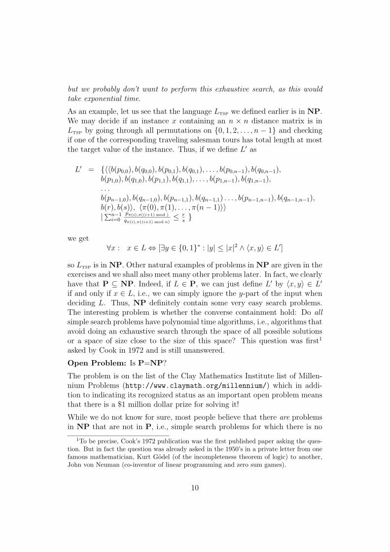
but we probably don’t want to perform this exhaustive search, as this wouldtake exponential time.

As an example, let us see that the language LTSP we defined earlier is in NP.We may decide if an instance x containing an n × n distance matrix is inLTSP by going through all permutations on {0, 1, 2, . . . , n − 1} and checkingif one of the corresponding traveling salesman tours has total length at mostthe target value of the instance. Thus, if we define L′ as

L′ = {〈〈b(p0,0), b(q0,0), b(p0,1), b(q0,1), . . . , b(p0,n−1), b(q0,n−1),b(p1,0), b(q1,0), b(p1,1), b(q1,1), . . . , b(p1,n−1), b(q1,n−1),. . .b(pn−1,0), b(qn−1,0), b(pn−1,1), b(qn−1,1) . . . , b(pn−1,n−1), b(qn−1,n−1),b(r), b(s)〉, 〈π(0), π(1), . . . , π(n− 1)〉〉|∑n−1

i=0pπ(i),π((i+1) mod )

qπ(i),π((i+1) mod n)≤ r

s}

we get∀x : x ∈ L ⇔ [∃y ∈ {0, 1}∗ : |y| ≤ |x|2 ∧ 〈x, y〉 ∈ L′]

so LTSP is in NP. Other natural examples of problems in NP are given in theexercises and we shall also meet many other problems later. In fact, we clearlyhave that P ⊆ NP. Indeed, if L ∈ P, we can just define L′ by 〈x, y〉 ∈ L′

if and only if x ∈ L, i.e., we can simply ignore the y-part of the input whendeciding L. Thus, NP definitely contain some very easy search problems.The interesting problem is whether the converse containment hold: Do allsimple search problems have polynomial time algorithms, i.e., algorithms thatavoid doing an exhaustive search through the space of all possible solutionsor a space of size close to the size of this space? This question was first1

asked by Cook in 1972 and is still unanswered.

Open Problem: Is P=NP?

The problem is on the list of the Clay Mathematics Institute list of Millen-nium Problems (http://www.claymath.org/millennium/) which in addi-tion to indicating its recognized status as an important open problem meansthat there is a $1 million dollar prize for solving it!

While we do not know for sure, most people believe that there are problemsin NP that are not in P, i.e., simple search problems for which there is no

1To be precise, Cook’s 1972 publication was the first published paper asking the ques-tion. But in fact the question was already asked in the 1950’s in a private letter from onefamous mathematician, Kurt Godel (of the incompleteness theorem of logic) to another,John von Neuman (co-inventor of linear programming and zero sum games).

10

efficient alternative to searching through an exponentially big search spaceof possible solutions. Their belief comes from the generality of the notion ofNP. In particular, consider the activity of mathematics, a substantial part ofwhich consists of finding proofs of theorems. While proofs as communicatedbetween mathematicians are informal, it is a well-established principle that aproof should be in principle formalizable. Also, set theory, as formalized bythe formal system ZFC (Zermelo-Frankel with the Axiom of Choice) is gener-ally accepted as a formal system strong enough to capture all of mainstreammathematics. Here, it is not important exactly what this formal system is,as we shall only use the following properties of it in our discussion: Theoremsand proofs in ZFC are strings over some finite alphabet Σ. By encoding eachsymbol of Σ as a string over {0, 1}, we can also think of theorems and proofsin ZFC as Boolean strings. Furthermore, given an alleged theorem string tand an alleged proof string p, we can decide in polynomial time in |t| + |p|if p really is a proof of t, i.e., formal proofs can be checked efficiently. Thecompelling evidence against P=NP is then this:

Proposition 2 If P=NP, then there is an algorithmic procedure that takesas input a formal statement t of ZFC and, if this statement has a proofin ZFC of length n, the procedure terminates in time polynomial in |t| + noutputting the shortest proof of t.

Proof Define MATH = {〈t, u(n), s〉| There is a ZFC-proof of length at mostn proving statement t and the proof begins with the string s} where u is theunary notation of integer n. We have that MATH ∈ NP, as we could searchthrough all strings s′ of length at most n− |s| and check for each of them ifs · s′ is a valid proof of t. Now, if P=NP, we also have that MATH is in P.This means that there is a polynomial time algorithm deciding MATH.

Now, let λ denote the empty string. Given t, run the efficient algorithm forMATH on inputs 〈t, u(1), λ〉, 〈t, u(2), λ〉, 〈t, u(3), λ〉, . . . until we find an n sothat 〈t, u(n), λ〉 is in MATH. We now know that the shortest proof of t haslength n. We can now find a proof of length n by a “binary search” procedure:We first check if 〈t, u(n), 0〉 is in MATH. If it is, we know that there is a proofof length n starting with 0 and we may then start figuring out the secondsymbol of the proof by checking if 〈t, u(n), 00〉 is in MATH. If 〈t, u(n), 0〉 isnot in MATH, we know that there is a proof of length n starting with 1 andwe then start to figure out the second symbol of the proof by checking if〈t, u(n), 10〉 is in MATH, etc. Each time we run the algorithm for MATHwe learn another symbol of the proof. Thus, by running the algorithm forMATH n additional times, we end up knowing the shortest proof of theoremt and can give it as output. This completes the proof of the proposition.

11

Why is Proposition 2 evidence against P=NP? The reason is this. Oftenproofs found by mathematicians are extremely ingenious, containing non-trivial and deep ideas and we celebrate these proofs and the people who findthem (in particular, we may give then one million dollar awards, like the Clayawards mentioned above). Even so, relatively short and elegant proofs maygo unnoticed for centuries. We certainly do not suspect that finding suchproofs may be automatized in a way that is efficient in the worst case., i.e.,that a Turing machine can find the shortest proof of any theorem in timepolynomial time in the length of the proof, no matter how tricky, deep andingenious it is! Hence we believe that P 6= NP.

4 Reductions and the complexity class NPC

Our interest in NP comes from the fact that the class contains many prob-lems we would like to solve. If we assume that P 6= NP, some of theseproblems cannot be solved by an efficient (i.e., polynomial time) algorithm.On the other hand, many problems in NP are easy, as P is a subset of NP. Ifwe have a particular problem at hand and have worked on it for a while with-out coming up with an efficient algorithm for the problem, we may begin tosuspect that it has no efficient algorithm. The concept of NP-completenessto be introduced in this section helps us converting this suspicion into aproven fact (under the assumption that P6=NP) and hence avoiding wastingtime trying to construct a worst case efficient algorithm that doesn’t exist!

We first need to formalize the notion of a reduction. Given two languages L1

and L2, we say that there is a reduction from L1 to L2 or alternatively thatL1 reduces to L2 and write L1 ≤ L2 if there is a polynomial time computablefunction r (the reduction) so that for all x ∈ {0, 1}∗, we have that x ∈ L1 ifand only if r(x) ∈ L2.

The ≤-notation suggests a partial order, which is slightly misleading: It isnot true that L1 ≤ L2 and L2 ≤ L1 implies L1 = L2 (why not?). On theother hand, reductions do satisfy the transitivity property:

Proposition 3 If L1 ≤ L2 and L2 ≤ L3 then L1 ≤ L3.

Proof We have a polynomial time computable map r1, r2 so that for all x,we have x ∈ L1 if and only if r1(x) ∈ L2 and for all y, we have y ∈ L2 if andonly if r2(y) ∈ L3. Hence, for all x, x ∈ L1 if and only if r2 ◦ r1(x) ∈ L3.Furthermore r2◦r1 is a polynomial time computable map and hence L1 ≤ L3.

12

A reduction r from L1 to L2 is, intuitively, just a translation of L1 instancesinto L2 instances: If we want to know the answer to an L1-instance x but onlyhave an algorithm for L2 running in time q(n) on inputs of length n, we maycompute r(x) and use the algorithm to get the answer using time q(|r(x)|).Appealing to the Polynomial Church-Turing thesis, we have established thefollowing formal statement:

Proposition 4 If L1 ≤ L2 and L2 ∈ P then L1 ∈ P.

We may think of L2 as being a more general language than L1 and henceless likely to be in P. Now suppose a language L2 has the property that forall L1 ∈ NP we have that L1 reduces to L2. Intuitively, such a language isless likely to be in P than any languages in NP. Formally, we call such alanguage NP-hard and capture the intuition in the following statement.

Proposition 5 Let L be an NP-hard language. If P 6= NP then L 6∈ P.

Proof That L is NP-hard means that ∀L′ ∈ NP : L′ ≤ L. If we assumeto the contrary that L is in P, then by Proposition 4, all L′ ∈ NP is in Pand hence P=NP.

NP-hard languages do not necessarily lie in NP. But we are particularlyinterested in those that do: We define the class NPC of NP-complete lan-guages to be those languages in NP that are NP-hard.

Proposition 6 Let L ∈ NPC. Then P=NP if and only if L is in P.

Proof Proposition 5 gives the “if” direction. The “only if” direction followsfrom L being in NP.

Getting back to the situation described in the beginning of the section: Hav-ing worked on a particular problem in NP and failed to find an efficientalgorithm, we might instead try to establish that the problem is in NPC. Ifwe do, and if we believe that P6= NP (perhaps convinced by the evidencein the preceeding section), we are now satisfied that no efficient algorithmexists. Even if we have no opinion about whether P6=NP, we at least knowthat constructing an efficient algorithm for our problem is a non-trivial task:Indeed, if we construct an algorithm and prove that it has polynomial worstcase time complexity, we have proved that P=NP and will be awarded onemillion dollars for our achievement by the Clay institute!

13

It is therefore of great interest to prove that natural problems in NP thatwe would like to solve but do not know an efficient algorithm for are NP-complete. A priori, it is not clear that this would be the case for very manyproblems (it is not perhaps not even clear that it is the case for any problem)and hence it is not clear that the definition of NPC would be very useful.Fortunately, it turns out that a substantial fraction of the natural problemsin NP that we do not know how to solve are NP-complete, and we shallbe able to prove this. However, if we use the definition of NPC for such aproof, we must prove that any problem in NP reduces to the problem weare interested in, and this may seem quite awkward to prove. To prove thata concrete problem is NP-hard, we shall usually use the following lemmainstead which makes it to sufficient to establish a single reduction.

Lemma 7 If L1 is NP-hard and L1 ≤ L2 then L2 is NP-hard.

Proof Since L1 is NP-hard, every language L in NP reduces to L1. SinceL1 reduces to L2, we may use Proposition 3 and conclude that every languageL in NP reduces to L2. Hence L2 is NP-hard, as desired.

Thus, when we establish that a certain problem is NP-complete, we canadd it to a “mental database” of such problems, and it becomes easier toestablish NP-completeness of new problems L in NP: We just need to findone problem in the database that we can reduce to L and we may appeal toLemma 7. Indeed, this is how we are going to operate. The tricky thing is toget the database started: We must establish one natural “mother” problemto be NP-complete. This was first done by Cook, in Cook’s Theorem tobe established in Section 6. To state and prove it, however, we must firstintroduce the notion of a Boolean circuit.

5 Boolean Circuits

For notational convenience, we shall make the well-known identification ofthe Boolean value true with 1 and the Boolean value false with 0 in thisand following sections.

A Boolean circuit with n input gates and m output gates is a directed, acyclicgraph G = (V, E). The vertices of V are called gates. Each gate has a labelwhich indicates the type of the gate. A label is either taken from the setof function symbols {AND,OR, NOT,COPY }, from the set of constantsymbols {0, 1} (representing false and true), or from the set of variable

14

symbols {X1, X2, . . . , Xn}. For each j, at most one gate is labeled Xj. Thegates labeled with a variable symbol are called input gates. We shall callgates labeled AND for AND-gates and use similar terminology for the othertypes of function gates. The arcs in E are called wires. If there is a wirefrom gate u to gate v, we say that u is an input to gate v. The followingconstraints must be satisfied:

1. Each AND-gate and OR-gate has exactly two inputs.

2. Each NOT-gate and COPY-gate has exactly one input.

3. The input gates are sources in G.

Finally, m of the gates are designated as output gates; we call these o1, o2, . . . , om.

A Boolean circuit C defines or computes a Boolean function from {0, 1}n to{0, 1}m in the following way: Given a vector x ∈ {0, 1}n, we can assign thevalue xi to each gate labeled Xi. The gates labeled 0 (1) are assigned theBoolean values 0 (1). Then, we iteratively assign values to the rest of thegates using the following rules.

1. Whenever the two inputs of an AND-gate have been assigned values,we assign the boolean AND of these two values to the gate.

2. Whenever the two inputs of an OR-gate have been assigned values, weassign the boolean OR of these two values to the gate.

3. Whenever the input of a NOT-gate has been assigned a value, we assignthe boolean negation of this value to the gate.

4. Whenever the input of a COPY-gate has been assigned a value, weassign the same value to the gate.

Since the circuit is acyclic and the only sources of the graph are assignedvalues when we begin, each gate in the circuit will eventually be assigned avalue. The value of the function on the input x is then the vector y ∈ {0, 1}m

obtained by collecting the values assigned to the output gates o1, o2, . . . , om.We refer to the entire process as evaluating the circuit on input x.

We shall abuse notation slightly and use the name C to denote both thecircuit and the function it is computing, i.e., we shall write C(x) = y.

Any Boolean function can be computed by some circuit:

15

Lemma 8 For any Boolean function f : {0, 1}n → {0, 1}m, there is a circuitC, so that ∀x ∈ {0, 1}n : C(x) = f(x).

Proof First, we can assume without loss of generality that m = 1, as we cancombine m 1-output circuits to get an m-output circuit. We also notice thatwe may view a Boolean formula such as (X1 ∨X2) ∧X3 as a special kind ofone-output Boolean circuit: One where each function gate is the input to atmost one other gate. Indeed, the graph induced by the function gates of sucha circuit is a tree, and we may identify it with the parse tree of the formula.Thus, we just have to show that any Boolean function f : {0, 1}n → {0, 1}can be defined by a Boolean formula with operations ∨,∧ ¬ and variablesX1, X2, . . . , Xn.

Given f : {0, 1}n → {0, 1}. For each x∗ ∈ f−1(1), we can define a formulagx∗ which evaluates to 1 on input x∗ and to 0 on all inputs, namely theconjunction (i.e., AND) of all variables that are true in x∗ and the negationsof all variables that are false in x∗. For instance, if x∗ = (1, 1, 0), we havegx∗ ≡ (X1 ∧ X2) ∧ ¬X3. The desired formula for f is then the disjunction(i.e., OR) of gx∗ over all x∗ ∈ f−1(1). This completes the proof.

Thus, we may regard circuits as low-level, but completely general compu-tational devices. However, unlike a Turing Machine, a circuit takes inputsof a fixed input length only. Circuits serve an important role in the theoryof NP-completeness because of their dual role of computational devices andas combinatorial objects that may be used as inputs to natural search andoptimization problems.

By the size of a circuit we shall mean the number of gates in the circuit. Thesize of a circuit is a measure of the time required to evaluate the circuit onan input. The following important lemma connects the time measure of theTuring machine model to the size measure of the circuit model.

Lemma 9 Let any Turing machine M running in time at most p(n) ≥ n oninputs of length n, where p is a polynomial, be given.

Then, given any fixed input length n, there is a circuit Cn of size at mostO(p(n)2) so that for all x ∈ {0, 1}n, Cn(x) = 1 if and only if M accepts x.

Furthermore, the function mapping 1n to a description of Cn is polynomialtime computable.

Before we begin the proof, let us convey its idea by noting that the statementof the lemma is in no way surprising: A Turing machines is a primitive versionof a real computer and real computers are actually made of Boolean circuits.

16

Thus, we really should just build a Turing machine using standard electroniccomponents2. The main obstacle for such a construction is the fact that thecircuits we consider are acyclic, while the circuits used to build real computerscontain feedback loops. Feedback loops are necessary in real computers forpractical reasons: Real computers have to operate without any (or only avery large) a priori upper bound on the computation time and we want tooperate them interactively and repeatedly give them new inputs and receivenew outputs, etc. For this to be possible the gates of a real computer mustbe reused at each clock cycle, i.e., at each step of the computation. Here, weshall be able to do without feedback loops in the circuit simply by having aseparate collection of gates for each step of the computation. As we knowthere will be at most p(n) steps, this will make the size of our circuit only apolynomial factor larger than if we were allowed to use feedback loop.

With this discussion in mind, we proceed with the proof.

Proof Consider the computation of M on some input of x of length n. AsM runs in time p(n) and starts with the tape head in the cell at position 0,it cannot touch any tape cell other than those at position −p(n), .., 0, .., p(n)during the computation. Any other cell will never see the head and willcontain the blank symbol # throughout the computation.

For a fixed input x, and each position i ∈ Z (though only positions between−p(n) and p(n) will be interesting) and each point in time t ∈ {0, . . . , p(n)},let us define ct,i to be the following collection of information, which we shallcall a cell state vector.

1. The symbol written in the tape cell at this point in time.

2. Whether or not the tape head is pointing to the tape cell at this pointin time.

3. If the tape head is indeed pointing to the tape cell at this point in time,we make a note of the state of the finite control.

A cell state vector is a finite amount of information and we may encode it,in some arbitrary but fixed way, as a bit string ct,i ∈ {0, 1}s, where s is somenumber that depends on M only (and not on x nor even n = |x|).Now the crucial observation is the following:

2And since this is the task at hand, the reader will now appreciate that we took thesimple Turing machine model as our model of computation, rather than a model closer torealistic computers!

17

Observation: Suppose we don’t know x (or even n = |x|). Then, for t > 1,we can determine ct,i from ct−1,i−1, ct−1,i and ct−1,i+1. In other words, thereis a fixed Boolean function h : {0, 1}3s → {0, 1}s, depending on M only (andnot x nor n = |x|), so that ct,i = h(ct−1,i−1 · ct−1,i · ct−1,i+1)

The validity of the observation follows directly from the operational seman-tics of the Turing machine model. By Proposition 8, there is a circuit Dcomputing h.

We shall also need the following circuits:

• A circuit E computing E : {0, 1} → {0, 1}s so that E(b) is a cell statevector representing a cell containing the symbol b ∈ {0, 1} and notcontaining the tape head. By Proposition 8, such a circuit E exists.

• A circuit F computing F : {0, 1}s → {0, 1} so that F (y) = 1 if andonly if y is a cell state vector representing a cell that does hold the tapehead and with the finite control of the Turing machine in the acceptingconfiguration. Again, by Proposition 8, such a circuit F exists.

The circuit Cn we have to construct to prove the lemma will essentiallyobtained simply by gluing together (2p(n) + 1)p(n) copies of D, n copies ofE and (2p(n) + 1) copies of F and letting the output of Cn be a disjunctionof the outputs of the copies of F . The formal details of the constructionthat now follows will be somewhat tedious (a completely formal proof thatthe construction is correct would be even more tedious and is omitted). Thereader is at this point invited to convince himself that the construction of Cn

can be done using the component just defined, by examining Figure 1. Theformal definition of Cn follows.

We are going to need some constant gates. In particular, we define a collec-tion B of constant gates Bi, i = 1, ..s so that Bi holds the i’th bit in the cellstate vector representing a blank cell without the head.

The circuit Cn will contain (2p(n) + 1)p(n) subcircuits Gt,i, one subcircuitfor each position i ∈ {−p(n), . . . , 0, . . . , p(n)} and each point in time t ∈{0, 1, . . . , p(n)}. The subcircuit Gt,i is intended to compute the state vectorct,i and is defined in the following way.

1. For t = 0 and any i between 1 and n, the subcircuit Gt,i is a copy ofE but with its single input gate replaced with a COPY gate taking itsinput from input gate Xi.

2. For t = 0 and i = 0 we make G0,0 a collection of constant gates B′,

18

Figure 1: The circuit Cn. Red lines represent “busses” containing s wires.Thanks to Johnni Winther for preparing the figure.

19

together representing the cell state vector of a blank cell that doescontain the head and with the finite control in the start state.

3. For t = 0 and i 6∈ {0, 1, . . . , n}, we make G0,i a copy of B, i.e. acollection of constant gates representing the cell state vector of a blankcell that does not contain the tape head.

4. For t ≥ 1 and any i between −p(n) and p(n), the subcircuit Gt,i is acopy of D but with input gates Xi replaced with COPY-gates in thefollowing way:

• Each COPY-gate replacing input gate Xi, i ∈ {1, . . . , s} takes asinput the i’th output gate of Gt−1,i−1, unless i − 1 < −p(n), inwhich case we let the gate take as input Bi.

• Each COPY-gate replacing input gate Xs+i, i ∈ {1, . . . , s} takesas input the i’th output gate of Gt−1,i,

• Each COPY-gate replacing input gate X2s+i, i ∈ {1, . . . , s} takesas input the i’th output gate of Gt−1,i+1, unless i + 1 > p(n), inwhich case we let the gate take as input Bi.

We now add 2p(n) + 1 copies of F , named Hj, j ∈ {−p(n), . . . , p(n)} tothe circuit Cn in the following way: We replace input gate Xi of Hj by aCOPY-gate, copying the i’th output gate of the subcircuit Gp(n),j. Finally,we construct a circuit A computing the OR of 2p(n) + 1 inputs - such acircuit can be made using 2(2p(n) + 1) − 1 binary OR-gates arranged in atree - and replace all the input gates of this circuit with COPY-gates, copyingthe output gates of Hj, j ∈ {−p(n), . . . , p(n)}.As output gate of Cn, we retain the single output gate of A (i.e., we do notmake the output gates of all the other subcircuits into output gates of Cn).

This completes the construction of Cn. Clearly, the size of Cn is as desired, byconstruction. Also by construction, Cn has the desired property: It outputs1 on input x if and only if the machine M accepts x. Furthermore, thecompletely regular nature of Cn makes it easy to make an efficient algorithmthat outputs a representation of Cn in time nO(1) given n: Such an algorithmcan have descriptions of the circuits D, E and F built in and then merelyhas to combine the the correct number of copies of these circuits in thecorrect way which is a simple task. Appealing to the Polynomial Church-Turing thesis, we have thus established that the function mapping 1n to adescription of Cn is polynomial time computable. This completes the proofof the lemma.

20

6 Cook’s Theorem

Given a set of symbols denoting Boolean variables, a literal is a variable orits negation. A clause is a disjunction of a number of literals. For instance,(X1 ∨ X2 ∨ ¬X3) is a clause involving the literals X1, X2 and ¬X3. AConjunctive Normal Form (CNF) formula is a conjunction of a number ofclauses. For instance, (X1 ∨X2 ∨¬X3)∧ (X3 ∨¬X1) is a CNF formula. TheSATISFIABILITY PROBLEM or SAT is the following decision problem:Given a CNF formula, decide if there is an assignment of truth values tothe variables of the formula so that the formula evaluates to true. Suchan assignment is referred to as a satisfying assignment of the formula. Forinstance, for the formula (X1 ∨X2 ∨¬X3)∧ (X3 ∨¬X1) the answer is “yes”,as, for instance, the assignment X1 = X2 = X3 = true makes the formulaevaluate to true. On the other hand, for the formula (X1 ∨ ¬X2) ∧ (X2 ∨¬X1)∧ (X1∨X2)∧ (¬X1∨¬X2), the answer is “no”, as all truth assignmentsmake this formula evaluate to false.

Historically, SAT is the mother of all NP-complete problem we alluded to inSection 4:

Theorem 10 (Cook, 1972) SAT ∈ NPC.

Cook proved the theorem by directly showing that all problems in NP re-duces to SAT. Having already studied Boolean circuits, we can make a some-what simpler proof by first showing that all problems in NP reduces to arelated problem, CIRCUIT SAT (Theorem 11) and then showing that CIR-CUIT SAT reduces to SAT (Proposition 12). Cook’s theorem then followsfrom Lemma 7 and the obvious fact that SAT is in NP. Thus, in these notes,it is actually CIRCUIT SAT that becomes the mother of all NP-completeproblems. CIRCUIT SAT is the following decision problem: Given a Booleancircuit C, is there a vector x so that C(x) = 1? That is, is there an assign-ment of Boolean values to the input gates of the circuit that will make theoutput gate of the circuit evaluate to 1? Such an assignment shall be referredto as a satisfying assignment of the circuit. Since a Boolean formula maybe regarded as a special kind of Boolean circuit, as explained in the proof ofLemma 8, SAT may be regarded as a special case of CIRCUIT SAT.

Theorem 11 CIRCUIT SAT ∈ NPC

Proof CIRCUIT SAT is clearly in NP. We need to show that it is NP-hard. Let L be a language in NP. We must show that there is a polynomial

21

time reduction r so that

∀x : x ∈ L ⇔ r(x) ∈ CIRCUIT SAT,

Since L is in NP, by definition there is a language L′ in P and a polynomialp, so

∀x : x ∈ L ⇔ [∃y ∈ {0, 1}∗ : |y| ≤ p(|x|) ∧ 〈x, y〉 ∈ L′]

Now we may define the reduction r as follows. The reduction should mapinstances of L to instances of CIRCUIT SAT, i.e., to descriptions of circuits.Given input x, the value of r(x) is going to be a description of a circuit Cwhich may be written as a disjunction C ≡ D0 ∨ D1 ∨ D2 . . . Dp(|x|), i.e.,the reduction should construct p(|x|) subcircuits and combine them usingp(|x|) − 1 OR-gates. Each subcircuit Di should take i Boolean inputs andshould evaluate to 1 on input y ∈ {0, 1}i if and only if 〈x, y〉 ∈ L′. If we canachieve this, we clearly have x ∈ L ⇔ C ∈ CIRCUIT SAT, as desired.

The subcircuit Di is defined as follows. Let M be a Turing machine decid-ing L′ in polynomial time. From Lemma 9, we have an efficient algorithmthat given an input length n, outputs a circuit Cn so that for all z, y with|〈z, y〉| = n, we have that Cn(〈z, y〉) = 1 if and only if M accepts 〈z, y〉. Letn = |〈x, 1i〉| = 2(|x| + i) + 2. The circuit Cn takes an input 〈z, y〉. By ourdefinition of 〈·, ·〉, the circuit Cn reads the input z using the input gates la-beled X1, X3, X5, . . . , X2|z|−1 Now we replace these input gates with constantgates so that input gate X2i−1 is replaced with a constant gate representingthe bit xi. Furthermore, we replace input gates labeled X2, X4, . . . , withconstant gates labeled 0 and input gates labeled X2|x|+2 and X2|x|+3 withconstant gates labeled 1. Informally speaking, we hardwire the input x intothe circuit. The circuit we obtain in this way is the circuit Di and it clearlyhas the right property.

The reduction r should construct the subcircuits D0, D1, . . . , Dp(|x|), combinethem using OR-gates and output a representation of the resulting circuit C.Appealing to the Polynomial Church-Turing thesis, we conclude that r is apolynomial time computable map and the proof of the theorem is complete.

Proposition 12 CIRCUIT SAT ≤ SAT

Proof Given a one-output circuit C we should define a CNF formulaf = r(C) so that f has a satisfying assignment if and only if C does and sothat r is a polynomial time computable map.

22

The CNF formula f has a variable for each gate g of C. For convenience, weshall abuse notation slightly and also refer to the variable of f as g.

The clauses of f are defined as follows:

For each AND-gate g of C taking as input gates h1 and h2 we add a set ofclauses to f logically equivalent to the statement g ⇔ (h1 ∧ h2), namely theclauses:

(¬g ∨ h1) ∧ (¬g ∨ h2) ∧ (g ∨ ¬h1 ∨ ¬h2).

For each OR-gate g of C taking as input gates h1 and h2 we add a set ofclauses to f logically equivalent to the statement g ⇔ (h1 ∨ h2), namely theclauses:

(g ∨ ¬h1) ∧ (g ∨ ¬h2) ∧ (¬g ∨ h1 ∨ h2).

For each NOT-gate g of C taking as input gate h we add a set of clauses tof logically equivalent to the statement g ⇔ ¬h, namely the clauses:

(g ∨ h) ∧ (¬g ∨ ¬h).

For each COPY-gate g of C taking as input gate h we add a set of clausesto f logically equivalent to the statement g ⇔ h, namely the clauses:

(g ∨ ¬h) ∧ (¬g ∨ h).

For each constant gate g of C labeled 0 we add a clause (¬g).

For each constant gate g of C labeled 1 we add a clause (g).

Finally, for the unique output gate g of C we add a clause (g).

The function f is the conjunction of all the clauses described above. Appeal-ing to the Polynomial Church-Turing thesis, the reduction r is seen to bepolynomial time computable. Also, we have that C is satisfiable if and onlyif f is satisfiable: Any truth assignment to the variables of f that makes allclauses true corresponds exactly to an evaluation of the circuit C makingthe output gate true and vice versa. This completes the proof of Theorem12.

Having now established Cook’s theorem, we have bootstrapped our databaseof known NP-complete problems: It now contains the problem SAT (and itsgeneralisation CIRCUIT SAT). In the weeks to come, we shall expand it byconstructing a tree of reductions to other problems with SAT being the root.

The fact that SAT is NP-complete is also a statement which is interestingin its own right and in fact somewhat philosophically intriguing. That a

23

Boolean formula f is unsatisfiable is equivalent to saying that its negation¬f is true for all truth assignments, i.e., that it is a theorem of propositionallogic. For instance, X ∨ ¬X is a theorem of propositional logic because¬(X ∨ ¬X) (which is equivalent to the CNF-formula (¬X) ∧ (X)) is notsatisfiable. Thus, an algorithm for SAT can be regarded as an automatizationof a very special kind of mathematical proof finding activity, namely theactivity of refuting statements of propositional logic (of a special form) byfinding counterexamples. But recall that MATH, as we defined it in theproof of Proposition 2 is in NP and since SAT is NP-complete, we have thatMATH ≤ SAT. Thus, if we want to completely automatize mathematicalproof finding in general, it is enough to automatize refuting statements ofpropositional logic by finding counterexamples. In other words, the latteractivity is as hard as the former. This is quite a surprising statement!

7 Exercises

Exercise 1 Recall that the Euclidean Traveling Salesman Problem is thespecial case of the TSP where the distances are actual Euclidean distancesbetween pairs of points. How can we formalize this special case as a language(in the sense of Section 1)? Is the formalization of the special case a specialcase of the general formalization? (and yes, this question does make sense....)

Exercise 2 Graphs can be represented by adjacency matrices or edge lists.Show how to formally represent adjacency matrices and edge lists as stringsand formally define languages corresponding to some decision problems con-cerning graphs you have previously encountered, such as “Given a directeda graph G and two vertices s and t, is there a path from s to t in G?”. Inthe exercises in the notes on integer linear programming, two optimizationproblems concerning graphs were defined, namely the maximum independentset problem and the minimum vertex coloring problems. Formally define thetwo associated decision problems.

Exercise 3 Formally define the languages LILP and LMILP associated to In-teger Linear Programming and Mixed Integer Linear Programming. Showthat LTSP ≤ LILP.

Exercise 4 Prove Proposition 1.

Exercise 5 Prove that the adjacency matrix and edge list representationsof graphs, formalized in Exercise 2 are good and polynomially equivalent.Also prove that binary and k-ary, k > 2, notation of integers are good andpolynomially equivalent. Prove that binary and unary notation of integers

24

are good but not polynomially equivalent.

Exercise 6 Show that the languages associated to the maximum independentset problem and the minimum vertex coloring problems (Exercise 2) are inNP.

Exercise 7 Can you prove that the languages LILP and LMILP of Exercise 3are in NP? If not, what is the obstacle? Let Bounded (M)ILP, be the specialcase of (M)ILP where each variable xi must have two associated constraintsxi ≤ ui and xi ≥ li for some integer constants li, ui and let LBILP and LBMILP bethe associated languages. Show that LBILP and LBMILP are in NP. Actually,is is also true that LILP and LMILP are in NP but the proof is somewhattechnical.

Exercise 8 Is it easy to see if the language associated to the EuclideanTraveling Salesman problem of Exercise 1 is in NP? Why not?

Exercise 9 Show that LBILP (Exercise 6) is NP-complete by a reductionfrom SAT.

25