package ‘eco’ - the comprehensive r archive network · eco 5 where y i and x i represent the...
TRANSCRIPT

Package ‘eco’August 1, 2017
Version 4.0-1
Date 2017-7-26
Title Ecological Inference in 2x2 Tables
Maintainer Ying Lu <[email protected]>
Depends R (>= 2.0), MASS, utils
Description Implements the Bayesian and likelihood methods proposedin Imai, Lu, and Strauss (2008 <DOI: 10.1093/pan/mpm017>) and(2011 <DOI:10.18637/jss.v042.i05>) for ecological inference in 2by 2 tables as well as the method of bounds introduced by Duncan andDavis (1953). The package fits both parametric and nonparametricmodels using either the Expectation-Maximization algorithms (forlikelihood models) or the Markov chain Monte Carlo algorithms (forBayesian models). For all models, the individual-level data can bedirectly incorporated into the estimation whenever such data are available.Along with in-sample and out-of-sample predictions, the package alsoprovides a functionality which allows one to quantify the effect of dataaggregation on parameter estimation and hypothesis testing under theparametric likelihood models.
LazyLoad yes
LazyData yes
License GPL (>= 2)
URL https://github.com/kosukeimai/eco
BugReports https://github.com/kosukeimai/eco/issues
RoxygenNote 6.0.1
NeedsCompilation yes
Author Kosuke Imai [aut],Ying Lu [aut, cre],Aaron Strauss [aut],Hubert Jin [ctb]
Repository CRAN
Date/Publication 2017-08-01 05:24:50 UTC
1

2 census
R topics documented:census . . . . . . . . . . . . . . . . . . . . . . . . . . . . . . . . . . . . . . . . . . . . 2eco . . . . . . . . . . . . . . . . . . . . . . . . . . . . . . . . . . . . . . . . . . . . . . 3ecoBD . . . . . . . . . . . . . . . . . . . . . . . . . . . . . . . . . . . . . . . . . . . . 6ecoML . . . . . . . . . . . . . . . . . . . . . . . . . . . . . . . . . . . . . . . . . . . . 9ecoNP . . . . . . . . . . . . . . . . . . . . . . . . . . . . . . . . . . . . . . . . . . . . 13forgnlit30 . . . . . . . . . . . . . . . . . . . . . . . . . . . . . . . . . . . . . . . . . . 17forgnlit30c . . . . . . . . . . . . . . . . . . . . . . . . . . . . . . . . . . . . . . . . . . 17housep88 . . . . . . . . . . . . . . . . . . . . . . . . . . . . . . . . . . . . . . . . . . 18predict.eco . . . . . . . . . . . . . . . . . . . . . . . . . . . . . . . . . . . . . . . . . . 18predict.ecoNP . . . . . . . . . . . . . . . . . . . . . . . . . . . . . . . . . . . . . . . . 20predict.ecoNPX . . . . . . . . . . . . . . . . . . . . . . . . . . . . . . . . . . . . . . . 21predict.ecoX . . . . . . . . . . . . . . . . . . . . . . . . . . . . . . . . . . . . . . . . . 22print.summary.eco . . . . . . . . . . . . . . . . . . . . . . . . . . . . . . . . . . . . . . 24print.summary.ecoML . . . . . . . . . . . . . . . . . . . . . . . . . . . . . . . . . . . . 25print.summary.ecoNP . . . . . . . . . . . . . . . . . . . . . . . . . . . . . . . . . . . . 26Qfun . . . . . . . . . . . . . . . . . . . . . . . . . . . . . . . . . . . . . . . . . . . . . 27reg . . . . . . . . . . . . . . . . . . . . . . . . . . . . . . . . . . . . . . . . . . . . . . 28summary.eco . . . . . . . . . . . . . . . . . . . . . . . . . . . . . . . . . . . . . . . . 29summary.ecoML . . . . . . . . . . . . . . . . . . . . . . . . . . . . . . . . . . . . . . 30summary.ecoNP . . . . . . . . . . . . . . . . . . . . . . . . . . . . . . . . . . . . . . . 31wallace . . . . . . . . . . . . . . . . . . . . . . . . . . . . . . . . . . . . . . . . . . . 33
Index 34
census Black Illiteracy Rates in 1910 US Census
Description
This data set contains the proportion of the residents who are black, the proportion of those who canread, the total population as well as the actual black literacy rate and white literacy rate for 1040counties in the US. The dataset was originally analyzed by Robinson (1950) at the state level. King(1997) recoded the 1910 census at county level. The data set only includes those who are older than10 years of age.
Format
A data frame containing 5 variables and 1040 observations
X numeric the proportion of Black residents in each countyY numeric the overall literacy rates in each countyN numeric the total number of residents in each countyW1 numeric the actual Black literacy rateW2 numeric the actual White literacy rate

eco 3
References
Robinson, W.S. (1950). “Ecological Correlations and the Behavior of Individuals.” American Soci-ological Review, vol. 15, pp.351-357.
King, G. (1997). “A Solution to the Ecological Inference Problem: Reconstructing Individual Be-havior from Aggregate Data”. Princeton University Press, Princeton, NJ.
eco Fitting the Parametric Bayesian Model of Ecological Inference in 2x2Tables
Description
eco is used to fit the parametric Bayesian model (based on a Normal/Inverse-Wishart prior) forecological inference in 2×2 tables via Markov chain Monte Carlo. It gives the in-sample predictionsas well as the estimates of the model parameters. The model and algorithm are described in Imai,Lu and Strauss (2008, 2011).
Usage
eco(formula, data = parent.frame(), N = NULL, supplement = NULL,context = FALSE, mu0 = 0, tau0 = 2, nu0 = 4, S0 = 10,mu.start = 0, Sigma.start = 10, parameter = TRUE, grid = FALSE,n.draws = 5000, burnin = 0, thin = 0, verbose = FALSE)
Arguments
formula A symbolic description of the model to be fit, specifying the column and rowmargins of 2×2 ecological tables. Y ~ X specifies Y as the column margin (e.g.,turnout) and X as the row margin (e.g., percent African-American). Details andspecific examples are given below.
data An optional data frame in which to interpret the variables in formula. Thedefault is the environment in which eco is called.
N An optional variable representing the size of the unit; e.g., the total number ofvoters. N needs to be a vector of same length as Y and X or a scalar.
supplement An optional matrix of supplemental data. The matrix has two columns, whichcontain additional individual-level data such as survey data for W1 and W2,respectively. If NULL, no additional individual-level data are included in themodel. The default is NULL.
context Logical. If TRUE, the contextual effect is also modeled, that is to assume the rowmarginX and the unknownW1 andW2 are correlated. See Imai, Lu and Strauss(2008, 2011) for details. The default is FALSE.
mu0 A scalar or a numeric vector that specifies the prior mean for the mean param-eter µ for (W1,W2) (or for (W1,W2, X) if context=TRUE). When the input ofmu0 is a scalar, its value will be repeated to yield a vector of the length of µ,otherwise, it needs to be a vector of same length as µ. When context=TRUE, thelength of µ is 3, otherwise it is 2. The default is 0.

4 eco
tau0 A positive integer representing the scale parameter of the Normal-Inverse Wishartprior for the mean and variance parameter (µ,Σ). The default is 2.
nu0 A positive integer representing the prior degrees of freedom of the Normal-Inverse Wishart prior for the mean and variance parameter (µ,Σ). The defaultis 4.
S0 A positive scalar or a positive definite matrix that specifies the prior scale matrixof the Normal-Inverse Wishart prior for the mean and variance parameter (µ,Σ). If it is a scalar, then the prior scale matrix will be a diagonal matrix with thesame dimensions as Σ and the diagonal elements all take value of S0, otherwiseS0 needs to have same dimensions as Σ. When context=TRUE, Σ is a 3 × 3matrix, otherwise, it is 2× 2. The default is 10.
mu.start A scalar or a numeric vector that specifies the starting values of the mean pa-rameter µ. If it is a scalar, then its value will be repeated to yield a vector ofthe length of µ, otherwise, it needs to be a vector of same length as µ. Whencontext=FALSE, the length of µ is 2, otherwise it is 3. The default is 0.
Sigma.start A scalar or a positive definite matrix that specified the starting value of the vari-ance matrix Σ. If it is a scalar, then the prior scale matrix will be a diagonalmatrix with the same dimensions as Σ and the diagonal elements all take valueof S0, otherwise S0 needs to have same dimensions as Σ. When context=TRUE,Σ is a 3× 3 matrix, otherwise, it is 2× 2. The default is 10.
parameter Logical. If TRUE, the Gibbs draws of the population parameters, µ and Σ, arereturned in addition to the in-sample predictions of the missing internal cells,W . The default is TRUE.
grid Logical. If TRUE, the grid method is used to sample W in the Gibbs sampler.If FALSE, the Metropolis algorithm is used where candidate draws are sampledfrom the uniform distribution on the tomography line for each unit. Note that thegrid method is significantly slower than the Metropolis algorithm. The defaultis FALSE.
n.draws A positive integer. The number of MCMC draws. The default is 5000.
burnin A positive integer. The burnin interval for the Markov chain; i.e. the number ofinitial draws that should not be stored. The default is 0.
thin A positive integer. The thinning interval for the Markov chain; i.e. the numberof Gibbs draws between the recorded values that are skipped. The default is 0.
verbose Logical. If TRUE, the progress of the Gibbs sampler is printed to the screen. Thedefault is FALSE.
Details
An example of 2× 2 ecological table for racial voting is given below:
black voters white votersvote W1i W2i Yinot vote 1−W1i 1−W2i 1− Yi
Xi 1−Xi

eco 5
where Yi and Xi represent the observed margins, and W1 and W2 are unknown variables. In thisexmaple, Yi is the turnout rate in the ith precint,Xi is the proproption of African American in the ithprecinct. The unknownsW1i an dW2i are the black and white turnout, respectively. All variables areproportions and hence bounded between 0 and 1. For each i, the following deterministic relationshipholds, Yi = XiW1i + (1−Xi)W2i.
Value
An object of class eco containing the following elements:
call The matched call.
X The row margin, X .
Y The column margin, Y .
N The size of each table, N .
burnin The number of initial burnin draws.
thin The thinning interval.
nu0 The prior degrees of freedom.
tau0 The prior scale parameter.
mu0 The prior mean.
S0 The prior scale matrix.
W A three dimensional array storing the posterior in-sample predictions ofW . Thefirst dimension indexes the Monte Carlo draws, the second dimension indexesthe columns of the table, and the third dimension represents the observations.
Wmin A numeric matrix storing the lower bounds of W .
Wmax A numeric matrix storing the upper bounds of W .
The following additional elements are included in the output when parameter = TRUE.
mu The posterior draws of the population mean parameter, µ.
Sigma The posterior draws of the population variance matrix, Σ.
Author(s)
Kosuke Imai, Department of Politics, Princeton University, <[email protected]>, http://imai.princeton.edu; Ying Lu,Center for Promoting Research Involving Innovative StatisticalMethodology (PRIISM), New York University, <[email protected]>
References
Imai, Kosuke, Ying Lu and Aaron Strauss. (2011). “eco: R Package for Ecological Inferencein 2x2 Tables” Journal of Statistical Software, Vol. 42, No. 5, pp. 1-23. available at http://imai.princeton.edu/software/eco.html
Imai, Kosuke, Ying Lu and Aaron Strauss. (2008). “Bayesian and Likelihood Inference for 2 x 2Ecological Tables: An Incomplete Data Approach” Political Analysis, Vol. 16, No. 1 (Winter), pp.41-69. available at http://imai.princeton.edu/research/eiall.html

6 ecoBD
See Also
ecoML, ecoNP, predict.eco, summary.eco
Examples
## load the registration data## Not run: data(reg)
## NOTE: convergence has not been properly assessed for the following## examples. See Imai, Lu and Strauss (2008, 2011) for more## complete analyses.
## fit the parametric model with the default prior specificationres <- eco(Y ~ X, data = reg, verbose = TRUE)## summarize the resultssummary(res)
## obtain out-of-sample predictionout <- predict(res, verbose = TRUE)## summarize the resultssummary(out)
## load the Robinson's census datadata(census)
## fit the parametric model with contextual effects and N## using the default prior specificationres1 <- eco(Y ~ X, N = N, context = TRUE, data = census, verbose = TRUE)## summarize the resultssummary(res1)
## obtain out-of-sample predictionout1 <- predict(res1, verbose = TRUE)## summarize the resultssummary(out1)
## End(Not run)
ecoBD Calculating the Bounds for Ecological Inference in RxC Tables
Description
ecoBD is used to calculate the bounds for missing internal cells of R×C ecological table. The datacan be entered either in the form of counts or proportions.

ecoBD 7
Usage
ecoBD(formula, data = parent.frame(), N = NULL)
Arguments
formula A symbolic description of ecological table to be used, specifying the columnand row margins of R × C ecological tables. Details and specific examples aregiven below.
data An optional data frame in which to interpret the variables in formula. Thedefault is the environment in which ecoBD is called.
N An optional variable representing the size of the unit; e.g., the total numberof voters. If formula is entered as counts and the last row and/or column isomitted, this input is necessary.
Details
The data may be entered either in the form of counts or proportions. If proportions are used,formula may omit the last row and/or column of tables, which can be calculated from the remainingmargins. For example, Y ~ X specifies Y as the first column margin and X as the first row margin in2× 2 tables. If counts are used, formula may omit the last row and/or column margin of the tableonly if N is supplied. In this example, the columns will be labeled as X and not X, and the rows willbe labeled as Y and not Y.
For larger tables, one can use cbind() and +. For example, cbind(Y1, Y2, Y3) ~ X1 + X2 + X3 + X4)specifies 3× 4 tables.
An R× C ecological table in the form of counts:
ni11 ni12 . . . ni1C ni1.ni21 ni22 . . . ni2C ni2.. . . . . . . . . . . . . . .niR1 niR2 . . . niRC niR.
ni.1 ni.2 . . . ni.C Ni
where nnr. and ni.c represent the observed margins, Ni represents the size of the table, and nircare unknown variables. Note that for each i, the following deterministic relationships hold; nir. =∑C
c=1 nirc for r = 1, . . . , R, and ni.c =∑R
r=1 nirc for c = 1, . . . , C. Then, each of the unknowninner cells can be bounded in the following manner,
max(0, nir. + ni.c −Ni) ≤ nirc ≤ min(nir., ni.c).
If the size of tables, N, is provided,
An R× C ecological table in the form of proportions:
Wi11 Wi12 . . . Wi1C Yi1Wi21 Wi22 . . . Wi2C Yi2. . . . . . . . . . . . . . .WiR1 WiR2 . . . WiRC YiRXi1 Xi2 . . . XiC
8 ecoBD
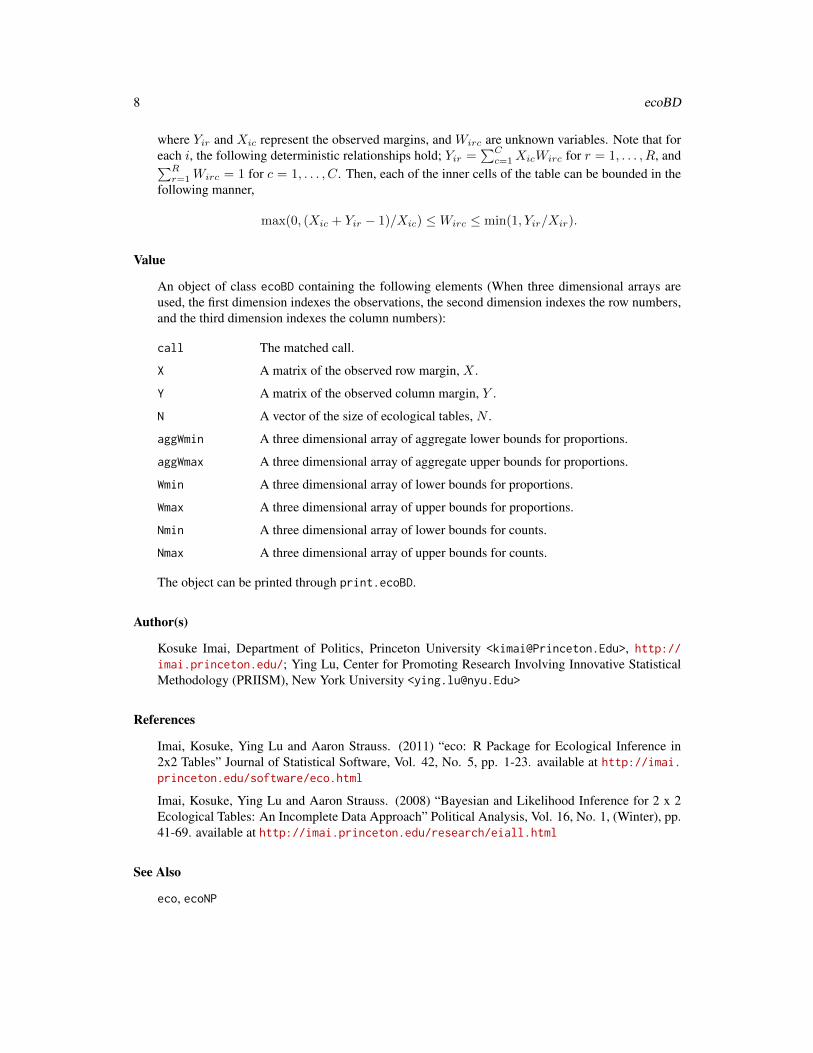
where Yir and Xic represent the observed margins, and Wirc are unknown variables. Note that foreach i, the following deterministic relationships hold; Yir =
∑Cc=1XicWirc for r = 1, . . . , R, and∑R
r=1Wirc = 1 for c = 1, . . . , C. Then, each of the inner cells of the table can be bounded in thefollowing manner,
max(0, (Xic + Yir − 1)/Xic) ≤Wirc ≤ min(1, Yir/Xir).
Value
An object of class ecoBD containing the following elements (When three dimensional arrays areused, the first dimension indexes the observations, the second dimension indexes the row numbers,and the third dimension indexes the column numbers):
call The matched call.
X A matrix of the observed row margin, X .
Y A matrix of the observed column margin, Y .
N A vector of the size of ecological tables, N .
aggWmin A three dimensional array of aggregate lower bounds for proportions.
aggWmax A three dimensional array of aggregate upper bounds for proportions.
Wmin A three dimensional array of lower bounds for proportions.
Wmax A three dimensional array of upper bounds for proportions.
Nmin A three dimensional array of lower bounds for counts.
Nmax A three dimensional array of upper bounds for counts.
The object can be printed through print.ecoBD.
Author(s)
Kosuke Imai, Department of Politics, Princeton University <[email protected]>, http://imai.princeton.edu/; Ying Lu, Center for Promoting Research Involving Innovative StatisticalMethodology (PRIISM), New York University <[email protected]>
References
Imai, Kosuke, Ying Lu and Aaron Strauss. (2011) “eco: R Package for Ecological Inference in2x2 Tables” Journal of Statistical Software, Vol. 42, No. 5, pp. 1-23. available at http://imai.princeton.edu/software/eco.html
Imai, Kosuke, Ying Lu and Aaron Strauss. (2008) “Bayesian and Likelihood Inference for 2 x 2Ecological Tables: An Incomplete Data Approach” Political Analysis, Vol. 16, No. 1, (Winter), pp.41-69. available at http://imai.princeton.edu/research/eiall.html
See Also
eco, ecoNP

ecoML 9
Examples
## load the registration datadata(reg)
## calculate the boundsres <- ecoBD(Y ~ X, N = N, data = reg)## print the resultsprint(res)
ecoML Fitting Parametric Models and Quantifying Missing Information forEcological Inference in 2x2 Tables
Description
ecoML is used to fit parametric models for ecological inference in 2 × 2 tables via ExpectationMaximization (EM) algorithms. The data is specified in proportions. At it’s most basic setting, thealgorithm assumes that the individual-level proportions (i.e., W1 and W2) and distributed bivariatenormally (after logit transformations). The function calculates point estimates of the parameters formodels based on different assumptions. The standard errors of the point estimates are also computedvia Supplemented EM algorithms. Moreover, ecoML quantifies the amount of missing informationassociated with each parameter and allows researcher to examine the impact of missing informationon parameter estimation in ecological inference. The models and algorithms are described in Imai,Lu and Strauss (2008, 2011).
Usage
ecoML(formula, data = parent.frame(), N = NULL, supplement = NULL,theta.start = c(0, 0, 1, 1, 0), fix.rho = FALSE, context = FALSE,sem = TRUE, epsilon = 10^(-6), maxit = 1000, loglik = TRUE,hyptest = FALSE, verbose = FALSE)
Arguments
formula A symbolic description of the model to be fit, specifying the column and rowmargins of 2×2 ecological tables. Y ~ X specifies Y as the column margin (e.g.,turnout) and X (e.g., percent African-American) as the row margin. Details andspecific examples are given below.
data An optional data frame in which to interpret the variables in formula. Thedefault is the environment in which ecoML is called.
N An optional variable representing the size of the unit; e.g., the total number ofvoters. N needs to be a vector of same length as Y and X or a scalar.

10 ecoML
supplement An optional matrix of supplemental data. The matrix has two columns, whichcontain additional individual-level data such as survey data for W1 and W2,respectively. If NULL, no additional individual-level data are included in themodel. The default is NULL.
theta.start A numeric vector that specifies the starting values for the mean, variance, andcovariance. When context = FALSE, the elements of theta.start correspondto (E(W1), E(W2), var(W1), var(W2), cor(W1,W2)). When context =TRUE, the elements of theta.start correspond to (E(W1), E(W2), var(W1),var(W2), corr(W1, X), corr(W2, X), corr(W1,W2)). Moreover, when fix.rho=TRUE,corr(W1,W2) is set to be the correlation betweenW1 andW2 when context = FALSE,and the partial correlation betweenW1 andW2 givenX when context = FALSE.The default is c(0,0,1,1,0).
fix.rho Logical. If TRUE, the correlation (when context=TRUE) or the partial correlation(when context=FALSE) between W1 and W2 is fixed through the estimation.For details, see Imai, Lu and Strauss(2006). The default is FALSE.
context Logical. If TRUE, the contextual effect is also modeled. In this case, the rowmargin (i.e., X) and the individual-level rates (i.e., W1 and W2) are assumedto be distributed tri-variate normally (after logit transformations). See Imai, Luand Strauss (2006) for details. The default is FALSE.
sem Logical. If TRUE, the standard errors of parameter estimates are estimated viaSEM algorithm, as well as the fraction of missing data. The default is TRUE.
epsilon A positive number that specifies the convergence criterion for EM algorithm.The square root of epsilon is the convergence criterion for SEM algorithm.The default is 10^(-6).
maxit A positive integer specifies the maximum number of iterations before the con-vergence criterion is met. The default is 1000.
loglik Logical. If TRUE, the value of the log-likelihood function at each iteration of EMis saved. The default is TRUE.
hyptest Logical. If TRUE, model is estimated under the null hypothesis that means ofW1 and W2 are the same. The default is FALSE.
verbose Logical. If TRUE, the progress of the EM and SEM algorithms is printed to thescreen. The default is FALSE.
Details
When SEM is TRUE, ecoML computes the observed-data information matrix for the parameters of in-terest based on Supplemented-EM algorithm. The inverse of the observed-data information matrixcan be used to estimate the variance-covariance matrix for the parameters estimated from EM algo-rithms. In addition, it also computes the expected complete-data information matrix. Based on thesetwo measures, one can further calculate the fraction of missing information associated with eachparameter. See Imai, Lu and Strauss (2006) for more details about fraction of missing information.
Moreover, when hytest=TRUE, ecoML allows to estimate the parametric model under the null hy-pothesis that mu_1=mu_2. One can then construct the likelihood ratio test to assess the hypothesisof equal means. The associated fraction of missing information for the test statistic can be alsocalculated. For details, see Imai, Lu and Strauss (2006) for details.

ecoML 11
Value
An object of class ecoML containing the following elements:
call The matched call.
X The row margin, X .
Y The column margin, Y .
N The size of each table, N .
context The assumption under which model is estimated. If context = FALSE, CARassumption is adopted and no contextual effect is modeled. If context = TRUE,NCAR assumption is adopted, and contextual effect is modeled.
sem Whether SEM algorithm is used to estimate the standard errors and observedinformation matrix for the parameter estimates.
fix.rho Whether the correlation or the partial correlation between W1 an W2 is fixed inthe estimation.
r12 If fix.rho = TRUE, the value that corr(W1,W2) is fixed to.
epsilon The precision criterion for EM convergence.√ε is the precision criterion for
SEM convergence.
theta.sem The ML estimates of E(W1),E(W2), var(W1),var(W2), and cov(W1,W2). Ifcontext = TRUE, E(X),cov(W1, X), cov(W2, X) are also reported.
W In-sample estimation of W1 and W2.
suff.stat The sufficient statistics for theta.em.
iters.em Number of EM iterations before convergence is achieved.
iters.sem Number of SEM iterations before convergence is achieved.
loglik The log-likelihood of the model when convergence is achieved.
loglik.log.em A vector saving the value of the log-likelihood function at each iteration of theEM algorithm.
mu.log.em A matrix saving the unweighted mean estimation of the logit-transformed individual-level proportions (i.e., W1 and W2) at each iteration of the EM process.
Sigma.log.em A matrix saving the log of the variance estimation of the logit-transformedindividual-level proportions (i.e., W1 and W2) at each iteration of EM process.Note, non-transformed variances are displayed on the screen (when verbose = TRUE).
rho.fisher.em A matrix saving the fisher transformation of the estimation of the correlationsbetween the logit-transformed individual-level proportions (i.e., W1 and W2) ateach iteration of EM process. Note, non-transformed correlations are displayedon the screen (when verbose = TRUE).
Moreover, when sem=TRUE, ecoML also output the following values:
DM The matrix characterizing the rates of convergence of the EM algorithms. Suchinformation is also used to calculate the observed-data information matrix
Icom The (expected) complete data information matrix estimated via SEM algorithm.When context=FALSE, fix.rho=TRUE, Icom is 4 by 4. When context=FALSE, fix.rho=FALSE,Icom is 5 by 5. When context=TRUE, Icom is 9 by 9.

12 ecoML
Iobs The observed information matrix. The dimension of Iobs is same as Icom.
Imiss The difference between Icom and Iobs. The dimension of Imiss is same asmiss.
Vobs The (symmetrized) variance-covariance matrix of the ML parameter estimates.The dimension of Vobs is same as Icom.
Iobs The (expected) complete-data variance-covariance matrix. The dimension ofIobs is same as Icom.
Vobs.original The estimated variance-covariance matrix of the ML parameter estimates. Thedimension of Vobs is same as Icom.
Fmis The fraction of missing information associated with each parameter estimation.
VFmis The proportion of increased variance associated with each parameter estimationdue to observed data.
Ieigen The largest eigen value of Imiss.
Icom.trans The complete data information matrix for the fisher transformed parameters.
Iobs.trans The observed data information matrix for the fisher transformed parameters.
Fmis.trans The fractions of missing information associated with the fisher transformed pa-rameters.
Author(s)
Kosuke Imai, Department of Politics, Princeton University, <[email protected]>, http://imai.princeton.edu; Ying Lu, Center for Promoting Research Involving Innovative StatisticalMethodology (PRIISM), New York University, <[email protected]>; Aaron Strauss, Departmentof Politics, Princeton University, <[email protected]>.
References
Imai, Kosuke, Ying Lu and Aaron Strauss. (2011). “eco: R Package for Ecological Inferencein 2x2 Tables” Journal of Statistical Software, Vol. 42, No. 5, pp. 1-23. available at http://imai.princeton.edu/software/eco.html
Imai, Kosuke, Ying Lu and Aaron Strauss. (2008). “Bayesian and Likelihood Inference for 2 x 2Ecological Tables: An Incomplete Data Approach” Political Analysis, Vol. 16, No. 1 (Winter), pp.41-69. available at http://imai.princeton.edu/research/eiall.html
See Also
eco, ecoNP, summary.ecoML
Examples
## load the census datadata(census)
## NOTE: convergence has not been properly assessed for the following

ecoNP 13
## examples. See Imai, Lu and Strauss (2006) for more complete analyses.## In the first example below, in the interest of time, only part of the## data set is analyzed and the convergence requirement is less stringent## than the default setting.
## In the second example, the program is arbitrarily halted 100 iterations## into the simulation, before convergence.
## load the Robinson's census datadata(census)
## fit the parametric model with the default model specifications## Not run: res <- ecoML(Y ~ X, data = census[1:100,], N=census[1:100,3],
epsilon=10^(-6), verbose = TRUE)## End(Not run)## summarize the results## Not run: summary(res)
## obtain out-of-sample prediction## Not run: out <- predict(res, verbose = TRUE)## summarize the results## Not run: summary(out)
## fit the parametric model with some individual## level data using the default prior specificationsurv <- 1:600## Not run: res1 <- ecoML(Y ~ X, context = TRUE, data = census[-surv,],
supplement = census[surv,c(4:5,1)], maxit=100, verbose = TRUE)## End(Not run)## summarize the results## Not run: summary(res1)
ecoNP Fitting the Nonparametric Bayesian Models of Ecological Inference in2x2 Tables
Description
ecoNP is used to fit the nonparametric Bayesian model (based on a Dirichlet process prior) forecological inference in 2 × 2 tables via Markov chain Monte Carlo. It gives the in-sample predic-tions as well as out-of-sample predictions for population inference. The models and algorithms aredescribed in Imai, Lu and Strauss (2008, 2011).
Usage
ecoNP(formula, data = parent.frame(), N = NULL, supplement = NULL,context = FALSE, mu0 = 0, tau0 = 2, nu0 = 4, S0 = 10,alpha = NULL, a0 = 1, b0 = 0.1, parameter = FALSE, grid = FALSE,n.draws = 5000, burnin = 0, thin = 0, verbose = FALSE)

14 ecoNP
Arguments
formula A symbolic description of the model to be fit, specifying the column and rowmargins of 2×2 ecological tables. Y ~ X specifies Y as the column margin (e.g.,turnout) and X as the row margin (e.g., percent African-American). Details andspecific examples are given below.
data An optional data frame in which to interpret the variables in formula. Thedefault is the environment in which ecoNP is called.
N An optional variable representing the size of the unit; e.g., the total number ofvoters. N needs to be a vector of same length as Y and X or a scalar.
supplement An optional matrix of supplemental data. The matrix has two columns, whichcontain additional individual-level data such as survey data for W1 and W2,respectively. If NULL, no additional individual-level data are included in themodel. The default is NULL.
context Logical. If TRUE, the contextual effect is also modeled, that is to assume the rowmarginX and the unknownW1 andW2 are correlated. See Imai, Lu and Strauss(2008, 2011) for details. The default is FALSE.
mu0 A scalar or a numeric vector that specifies the prior mean for the mean parameterµ of the base prior distribution G0 (see Imai, Lu and Strauss (2008, 2011) fordetailed descriptions of Dirichlete prior and the normal base prior distribution) .If it is a scalar, then its value will be repeated to yield a vector of the length of µ,otherwise, it needs to be a vector of same length as µ. When context=TRUE ,the length of µ is 3, otherwise it is 2. The default is 0.
tau0 A positive integer representing the scale parameter of the Normal-Inverse Wishartprior for the mean and variance parameter (µi,Σi) of each observation. The de-fault is 2.
nu0 A positive integer representing the prior degrees of freedom of the variance ma-trix Σi. the default is 4.
S0 A positive scalar or a positive definite matrix that specifies the prior scale matrixfor the variance matrix Σi. If it is a scalar, then the prior scale matrix will bea diagonal matrix with the same dimensions as Σi and the diagonal elementsall take value of S0, otherwise S0 needs to have same dimensions as Σi. Whencontext=TRUE, Σ is a 3× 3 matrix, otherwise, it is 2× 2. The default is 10.
alpha A positive scalar representing a user-specified fixed value of the concentrationparameter, α. If NULL, α will be updated at each Gibbs draw, and its priorparameters a0 and b0 need to be specified. The default is NULL.
a0 A positive integer representing the value of shape parameter of the gamma priordistribution for α. The default is 1.
b0 A positive integer representing the value of the scale parameter of the gammaprior distribution for α. The default is 0.1.
parameter Logical. If TRUE, the Gibbs draws of the population parameters, µ and Σ, arereturned in addition to the in-sample predictions of the missing internal cells,W . The default is FALSE. This needs to be set to TRUE if one wishes to makepopulation inferences through predict.eco. See an example below.

ecoNP 15
grid Logical. If TRUE, the grid method is used to sample W in the Gibbs sampler.If FALSE, the Metropolis algorithm is used where candidate draws are sampledfrom the uniform distribution on the tomography line for each unit. Note thatthe grid method is significantly slower than the Metropolis algorithm.
n.draws A positive integer. The number of MCMC draws. The default is 5000.
burnin A positive integer. The burnin interval for the Markov chain; i.e. the number ofinitial draws that should not be stored. The default is 0.
thin A positive integer. The thinning interval for the Markov chain; i.e. the numberof Gibbs draws between the recorded values that are skipped. The default is 0.
verbose Logical. If TRUE, the progress of the Gibbs sampler is printed to the screen. Thedefault is FALSE.
Value
An object of class ecoNP containing the following elements:
call The matched call.
X The row margin, X .
Y The column margin, Y .
burnin The number of initial burnin draws.
thin The thinning interval.
nu0 The prior degrees of freedom.
tau0 The prior scale parameter.
mu0 The prior mean.
S0 The prior scale matrix.
a0 The prior shape parameter.
b0 The prior scale parameter.
W A three dimensional array storing the posterior in-sample predictions ofW . Thefirst dimension indexes the Monte Carlo draws, the second dimension indexesthe columns of the table, and the third dimension represents the observations.
Wmin A numeric matrix storing the lower bounds of W .
Wmax A numeric matrix storing the upper bounds of W .
The following additional elements are included in the output when parameter = TRUE.
mu A three dimensional array storing the posterior draws of the population meanparameter, µ. The first dimension indexes the Monte Carlo draws, the seconddimension indexes the columns of the table, and the third dimension representsthe observations.
Sigma A three dimensional array storing the posterior draws of the population vari-ance matrix, Σ. The first dimension indexes the Monte Carlo draws, the seconddimension indexes the parameters, and the third dimension represents the obser-vations.
alpha The posterior draws of α.
nstar The number of clusters at each Gibbs draw.

16 ecoNP
Author(s)
Kosuke Imai, Department of Politics, Princeton University, <[email protected]>, http://imai.princeton.edu; Ying Lu, Center for Promoting Research Involving Innovative StatisticalMethodology (PRIISM), New York University <[email protected]>
References
Imai, Kosuke, Ying Lu and Aaron Strauss. (2011). “eco: R Package for Ecological Inferencein 2x2 Tables” Journal of Statistical Software, Vol. 42, No. 5, pp. 1-23. available at http://imai.princeton.edu/software/eco.html
Imai, Kosuke, Ying Lu and Aaron Strauss. (2008). “Bayesian and Likelihood Inference for 2 x 2Ecological Tables: An Incomplete Data Approach” Political Analysis, Vol. 16, No. 1 (Winter), pp.41-69. available at http://imai.princeton.edu/research/eiall.html
See Also
eco, ecoML, predict.eco, summary.ecoNP
Examples
## load the registration datadata(reg)
## NOTE: We set the number of MCMC draws to be a very small number in## the following examples; i.e., convergence has not been properly## assessed. See Imai, Lu and Strauss (2006) for more complete examples.
## fit the nonparametric model to give in-sample predictions## store the parameters to make population inference later## Not run: res <- ecoNP(Y ~ X, data = reg, n.draws = 50, param = TRUE, verbose = TRUE)
##summarize the resultssummary(res)
## obtain out-of-sample predictionout <- predict(res, verbose = TRUE)
## summarize the resultssummary(out)
## density plots of the out-of-sample predictionspar(mfrow=c(2,1))plot(density(out[,1]), main = "W1")plot(density(out[,2]), main = "W2")
## load the Robinson's census datadata(census)

forgnlit30c 17
## fit the parametric model with contextual effects and N## using the default prior specification
res1 <- ecoNP(Y ~ X, N = N, context = TRUE, param = TRUE, data = census,n.draws = 25, verbose = TRUE)
## summarize the resultssummary(res1)
## out-of sample predictionpres1 <- predict(res1)summary(pres1)## End(Not run)
forgnlit30 Foreign-born literacy in 1930
Description
This data set contains, on a state level, the proportion of white residents ten years and older whoare foreign born, and the proportion of those residents who are literate. Data come from the 1930census and were first analyzed by Robinson (1950).
Format
A data frame containing 5 variables and 48 observations
X numeric proportion of the white population at least 10 years of age that is foreign bornY numeric proportion of the white population at least 10 years of age that is illiterateW1 numeric proportion of the foreign-born white population at least 10 years of age that is illiterateW2 numeric proportion of the native-born white population at least 10 years of age that is illiterateICPSR numeric the ICPSR state code
References
Robinson, W.S. (1950). “Ecological Correlations and the Behavior of Individuals.” American Soci-ological Review, vol. 15, pp.351-357.
forgnlit30c Foreign-born literacy in 1930, County Level
Description
This data set contains, on a county level, the proportion of white residents ten years and older whoare foreign born, and the proportion of those residents who are literate. Data come from the 1930census and were first analyzed by Robinson (1950). Counties with fewer than 100 foreign bornresidents are dropped.
18 predict.eco
Format
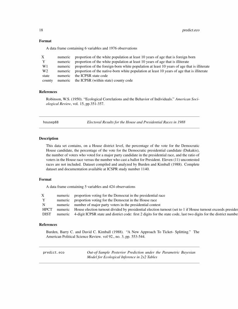
A data frame containing 6 variables and 1976 observations
X numeric proportion of the white population at least 10 years of age that is foreign bornY numeric proportion of the white population at least 10 years of age that is illiterateW1 numeric proportion of the foreign-born white population at least 10 years of age that is illiterateW2 numeric proportion of the native-born white population at least 10 years of age that is illiteratestate numeric the ICPSR state codecounty numeric the ICPSR (within state) county code
References
Robinson, W.S. (1950). “Ecological Correlations and the Behavior of Individuals.” American Soci-ological Review, vol. 15, pp.351-357.
housep88 Electoral Results for the House and Presidential Races in 1988
Description
This data set contains, on a House district level, the percentage of the vote for the DemocraticHouse candidate, the percentage of the vote for the Democratic presidential candidate (Dukakis),the number of voters who voted for a major party candidate in the presidential race, and the ratio ofvoters in the House race versus the number who cast a ballot for President. Eleven (11) uncontestedraces are not included. Dataset compiled and analyzed by Burden and Kimball (1988). Completedataset and documentation available at ICSPR study number 1140.
Format
A data frame containing 5 variables and 424 observations
X numeric proportion voting for the Democrat in the presidential raceY numeric proportion voting for the Democrat in the House raceN numeric number of major party voters in the presidential contestHPCT numeric House election turnout divided by presidential election turnout (set to 1 if House turnout exceeds presidential turnout)DIST numeric 4-digit ICPSR state and district code: first 2 digits for the state code, last two digits for the district number (e.g., 2106=IL 6th)
References
Burden, Barry C. and David C. Kimball (1988). “A New Approach To Ticket- Splitting.” TheAmerican Political Science Review. vol 92., no. 3, pp. 553-544.
predict.eco Out-of-Sample Posterior Prediction under the Parametric BayesianModel for Ecological Inference in 2x2 Tables

predict.eco 19
Description
Obtains out-of-sample posterior predictions under the fitted parametric Bayesian model for ecolog-ical inference. predict method for class eco and ecoX.
Usage
## S3 method for class 'eco'predict(object, newdraw = NULL, subset = NULL,verbose = FALSE, ...)
Arguments
object An output object from eco or ecoNP.
newdraw An optional list containing two matrices (or three dimensional arrays for thenonparametric model) of MCMC draws of µ and Σ. Those elements should benamed as mu and Sigma, respectively. The default is the original MCMC drawsstored in object.
subset A scalar or numerical vector specifying the row number(s) of mu and Sigma inthe output object from eco. If specified, the posterior draws of parameters forthose rows are used for posterior prediction. The default is NULL where all theposterior draws are used.
verbose logical. If TRUE, helpful messages along with a progress report on the MonteCarlo sampling from the posterior predictive distributions are printed on thescreen. The default is FALSE.
... further arguments passed to or from other methods.
Details
The posterior predictive values are computed using the Monte Carlo sample stored in the eco output(or other sample if newdraw is specified). Given each Monte Carlo sample of the parameters,we sample the vector-valued latent variable from the appropriate multivariate Normal distribution.Then, we apply the inverse logit transformation to obtain the predictive values of proportions, W .The computation may be slow (especially for the nonparametric model) if a large Monte Carlosample of the model parameters is used. In either case, setting verbose = TRUE may be helpful inmonitoring the progress of the code.
Value
predict.eco yields a matrix of class predict.eco containing the Monte Carlo sample from theposterior predictive distribution of inner cells of ecological tables. summary.predict.eco willsummarize the output, and print.summary.predict.eco will print the summary.
Author(s)
Kosuke Imai, Department of Politics, Princeton University, <[email protected]>, http://imai.princeton.edu; Ying Lu, Center for Promoting Research Involving Innovative StatisticalMethodology (PRIISM), New York University <[email protected]>
20 predict.ecoNP
See Also
eco, predict.ecoNP
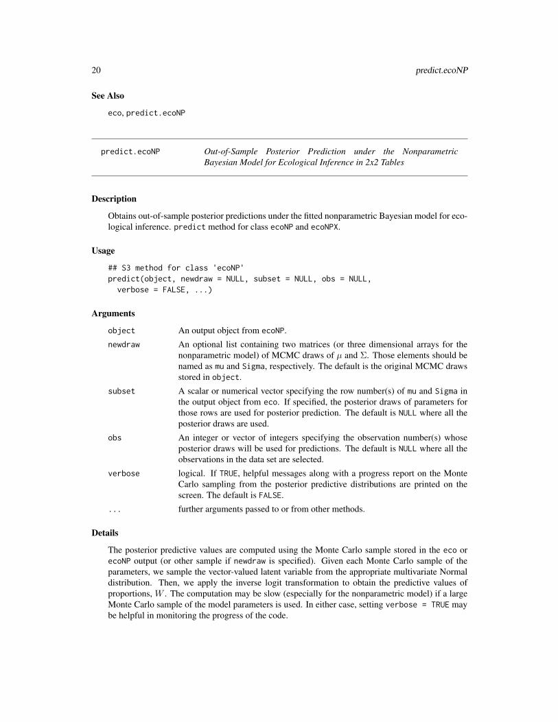
predict.ecoNP Out-of-Sample Posterior Prediction under the NonparametricBayesian Model for Ecological Inference in 2x2 Tables
Description
Obtains out-of-sample posterior predictions under the fitted nonparametric Bayesian model for eco-logical inference. predict method for class ecoNP and ecoNPX.
Usage
## S3 method for class 'ecoNP'predict(object, newdraw = NULL, subset = NULL, obs = NULL,verbose = FALSE, ...)
Arguments
object An output object from ecoNP.
newdraw An optional list containing two matrices (or three dimensional arrays for thenonparametric model) of MCMC draws of µ and Σ. Those elements should benamed as mu and Sigma, respectively. The default is the original MCMC drawsstored in object.
subset A scalar or numerical vector specifying the row number(s) of mu and Sigma inthe output object from eco. If specified, the posterior draws of parameters forthose rows are used for posterior prediction. The default is NULL where all theposterior draws are used.
obs An integer or vector of integers specifying the observation number(s) whoseposterior draws will be used for predictions. The default is NULL where all theobservations in the data set are selected.
verbose logical. If TRUE, helpful messages along with a progress report on the MonteCarlo sampling from the posterior predictive distributions are printed on thescreen. The default is FALSE.
... further arguments passed to or from other methods.
Details
The posterior predictive values are computed using the Monte Carlo sample stored in the eco orecoNP output (or other sample if newdraw is specified). Given each Monte Carlo sample of theparameters, we sample the vector-valued latent variable from the appropriate multivariate Normaldistribution. Then, we apply the inverse logit transformation to obtain the predictive values ofproportions, W . The computation may be slow (especially for the nonparametric model) if a largeMonte Carlo sample of the model parameters is used. In either case, setting verbose = TRUE maybe helpful in monitoring the progress of the code.

predict.ecoNPX 21
Value
predict.eco yields a matrix of class predict.eco containing the Monte Carlo sample from theposterior predictive distribution of inner cells of ecological tables. summary.predict.eco willsummarize the output, and print.summary.predict.eco will print the summary.
Author(s)
Kosuke Imai, Department of Politics, Princeton University, <[email protected]>, http://imai.princeton.edu; Ying Lu, Center for Promoting Research Involving Innovative StatisticalMethodology (PRIISM), New York University <[email protected]>
See Also
eco, ecoNP, summary.eco, summary.ecoNP
predict.ecoNPX Out-of-Sample Posterior Prediction under the NonparametricBayesian Model for Ecological Inference in 2x2 Tables
Description
Obtains out-of-sample posterior predictions under the fitted nonparametric Bayesian model for eco-logical inference. predict method for class ecoNP and ecoNPX.
Usage
## S3 method for class 'ecoNPX'predict(object, newdraw = NULL, subset = NULL,obs = NULL, cond = FALSE, verbose = FALSE, ...)
Arguments
object An output object from ecoNP.
newdraw An optional list containing two matrices (or three dimensional arrays for thenonparametric model) of MCMC draws of µ and Σ. Those elements should benamed as mu and Sigma, respectively. The default is the original MCMC drawsstored in object.
subset A scalar or numerical vector specifying the row number(s) of mu and Sigma inthe output object from eco. If specified, the posterior draws of parameters forthose rows are used for posterior prediction. The default is NULL where all theposterior draws are used.
obs An integer or vector of integers specifying the observation number(s) whoseposterior draws will be used for predictions. The default is NULL where all theobservations in the data set are selected.
cond logical. If TRUE, then the conditional prediction will made for the parametricmodel with contextual effects. The default is FALSE.
22 predict.ecoX
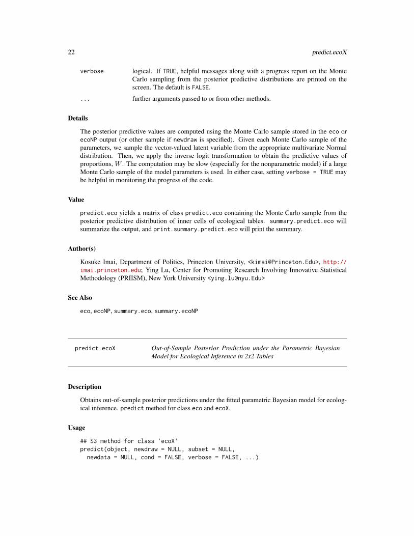
verbose logical. If TRUE, helpful messages along with a progress report on the MonteCarlo sampling from the posterior predictive distributions are printed on thescreen. The default is FALSE.
... further arguments passed to or from other methods.
Details
The posterior predictive values are computed using the Monte Carlo sample stored in the eco orecoNP output (or other sample if newdraw is specified). Given each Monte Carlo sample of theparameters, we sample the vector-valued latent variable from the appropriate multivariate Normaldistribution. Then, we apply the inverse logit transformation to obtain the predictive values ofproportions, W . The computation may be slow (especially for the nonparametric model) if a largeMonte Carlo sample of the model parameters is used. In either case, setting verbose = TRUE maybe helpful in monitoring the progress of the code.
Value
predict.eco yields a matrix of class predict.eco containing the Monte Carlo sample from theposterior predictive distribution of inner cells of ecological tables. summary.predict.eco willsummarize the output, and print.summary.predict.eco will print the summary.
Author(s)
Kosuke Imai, Department of Politics, Princeton University, <[email protected]>, http://imai.princeton.edu; Ying Lu, Center for Promoting Research Involving Innovative StatisticalMethodology (PRIISM), New York University <[email protected]>
See Also
eco, ecoNP, summary.eco, summary.ecoNP
predict.ecoX Out-of-Sample Posterior Prediction under the Parametric BayesianModel for Ecological Inference in 2x2 Tables
Description
Obtains out-of-sample posterior predictions under the fitted parametric Bayesian model for ecolog-ical inference. predict method for class eco and ecoX.
Usage
## S3 method for class 'ecoX'predict(object, newdraw = NULL, subset = NULL,newdata = NULL, cond = FALSE, verbose = FALSE, ...)

predict.ecoX 23
Arguments
object An output object from eco or ecoNP.
newdraw An optional list containing two matrices (or three dimensional arrays for thenonparametric model) of MCMC draws of µ and Σ. Those elements should benamed as mu and Sigma, respectively. The default is the original MCMC drawsstored in object.
subset A scalar or numerical vector specifying the row number(s) of mu and Sigma inthe output object from eco. If specified, the posterior draws of parameters forthose rows are used for posterior prediction. The default is NULL where all theposterior draws are used.
newdata An optional data frame containing a new data set for which posterior predictionswill be made. The new data set must have the same variable names as those inthe original data.
cond logical. If TRUE, then the conditional prediction will made for the parametricmodel with contextual effects. The default is FALSE.
verbose logical. If TRUE, helpful messages along with a progress report on the MonteCarlo sampling from the posterior predictive distributions are printed on thescreen. The default is FALSE.
... further arguments passed to or from other methods.
Details
The posterior predictive values are computed using the Monte Carlo sample stored in the eco output(or other sample if newdraw is specified). Given each Monte Carlo sample of the parameters,we sample the vector-valued latent variable from the appropriate multivariate Normal distribution.Then, we apply the inverse logit transformation to obtain the predictive values of proportions, W .The computation may be slow (especially for the nonparametric model) if a large Monte Carlosample of the model parameters is used. In either case, setting verbose = TRUE may be helpful inmonitoring the progress of the code.
Value
predict.eco yields a matrix of class predict.eco containing the Monte Carlo sample from theposterior predictive distribution of inner cells of ecological tables. summary.predict.eco willsummarize the output, and print.summary.predict.eco will print the summary.
Author(s)
Kosuke Imai, Department of Politics, Princeton University, <[email protected]>, http://imai.princeton.edu; Ying Lu, Center for Promoting Research Involving Innovative StatisticalMethodology (PRIISM), New York University <[email protected]>
See Also
eco, predict.ecoNP

24 print.summary.eco
print.summary.eco Print the Summary of the Results for the Bayesian Parametric Modelfor Ecological Inference in 2x2 Tables
Description
summary method for class eco.
Usage
## S3 method for class 'summary.eco'print(x, digits = max(3, getOption("digits") - 3), ...)
Arguments
x An object of class summary.eco.digits the number of significant digits to use when printing.... further arguments passed to or from other methods.
Value
summary.eco yields an object of class summary.eco containing the following elements:
call The call from eco.n.obs The number of units.n.draws The number of Monte Carlo samples.agg.table Aggregate posterior estimates of the marginal means of W1 and W2 using X
and N as weights.
If param = TRUE, the following elements are also included:
param.table Posterior estimates of model parameters: population mean estimates of W1 andW2 and their logit transformations.
If units = TRUE, the following elements are also included:
W1.table Unit-level posterior estimates for W1.W2.table Unit-level posterior estimates for W2.
This object can be printed by print.summary.eco
Author(s)
Kosuke Imai, Department of Politics, Princeton University, <[email protected]>, http://imai.princeton.edu; Ying Lu, Center for Promoting Research Involving Innovative StatisticalMethodology (PRIISM), New York University <[email protected]>
See Also
eco, predict.eco

print.summary.ecoML 25
print.summary.ecoML Print the Summary of the Results for the Maximum Likelihood Para-metric Model for Ecological Inference in 2x2 Tables
Description
summary method for class eco.
Usage
## S3 method for class 'summary.ecoML'print(x, digits = max(3, getOption("digits") - 3),...)
Arguments
x An object of class summary.ecoML.
digits the number of significant digits to use when printing.
... further arguments passed to or from other methods.
Value
summary.eco yields an object of class summary.eco containing the following elements:
call The call from eco.
sem Whether the SEM algorithm was executed, as specified by the user upon callingecoML.
fix.rho Whether the correlation parameter was fixed or allowed to vary, as specified bythe user upon calling ecoML.
epsilon The convergence threshold specified by the user upon calling ecoML.
n.obs The number of units.
iters.em The number iterations the EM algorithm cycled through before convergence orreaching the maximum number of iterations allowed.
iters.sem The number iterations the SEM algorithm cycled through before convergence orreaching the maximum number of iterations allowed.
loglik The final observed log-likelihood.
rho A matrix of iters.em rows specifying the correlation parameters at each it-eration of the EM algorithm. The number of columns depends on how manycorrelation parameters exist in the model. Column order is the same as the orderof the parameters in param.table.
param.table Final estimates of the parameter values for the model. Excludes parametersfixed by the user upon calling ecoML. See ecoML documentation for order ofparameters.
agg.table Aggregate estimates of the marginal means of W1 and W2

26 print.summary.ecoNP
agg.wtable Aggregate estimates of the marginal means of W1 and W2 using X and N asweights.
If units = TRUE, the following elements are also included:
W.table Unit-level estimates for W1 and W2.
This object can be printed by print.summary.eco
Author(s)
Kosuke Imai, Department of Politics, Princeton University, <[email protected]>, http://imai.princeton.edu; Ying Lu, Center for Promoting Research Involving Innovative StatisticalMethodology (PRIISM), New York University <[email protected]>; Aaron Strauss, Departmentof Politics, Princeton University, <[email protected]>
See Also
ecoML
print.summary.ecoNP Print the Summary of the Results for the Bayesian NonparametricModel for Ecological Inference in 2x2 Tables
Description
summary method for class ecoNP.
Usage
## S3 method for class 'summary.ecoNP'print(x, digits = max(3, getOption("digits") - 3),...)
Arguments
x An object of class summary.ecoNP.
digits the number of significant digits to use when printing.
... further arguments passed to or from other methods.
Value
summary.ecoNP yields an object of class summary.ecoNP containing the following elements:
call The call from ecoNP.
n.obs The number of units.
n.draws The number of Monte Carlo samples.

Qfun 27
agg.table Aggregate posterior estimates of the marginal means of W1 and W2 using Xand N as weights.
If param = TRUE, the following elements are also included:
param.table Posterior estimates of model parameters: population mean estimates of W1 andW2. If subset is specified, only a subset of the population parameters are in-cluded.
If unit = TRUE, the following elements are also included:
W1.table Unit-level posterior estimates for W1.
W2.table Unit-level posterior estimates for W2.
This object can be printed by print.summary.ecoNP
Author(s)
Kosuke Imai, Department of Politics, Princeton University, <[email protected]>, http://imai.princeton.edu; Ying Lu, Center for Promoting Research Involving Innovative StatisticalMethodology (PRIISM), New York University <[email protected]>
See Also
ecoNP, predict.eco
Qfun Fitting the Parametric Bayesian Model of Ecological Inference in 2x2Tables
Description
Qfun returns the complete log-likelihood that is used to calculate the fraction of missing informa-tion.
Usage
Qfun(theta, suff.stat, n)
Arguments
theta A vector that contains the MLEE(W1),E(W2), var(W1),var(W2), and cov(W1,W2).Typically it is the element theta.em of an object of class ecoML.
suff.stat A vector of sufficient statistics of E(W1), E(W2), var(W1),var(W2), andcov(W1,W2).
n A integer representing the sample size.

28 reg
Author(s)
Kosuke Imai, Department of Politics, Princeton University, <[email protected]>, http://imai.princeton.edu; Ying Lu, Center for Promoting Research Involving Innovative StatisticalMethodology (PRIISM), New York University <[email protected]> Aaron Strauss, Department ofPolitics, Princeton University, <[email protected]>.
References
Imai, Kosuke, Ying Lu and Aaron Strauss. (2011). “eco: R Package for Ecological Inferencein 2x2 Tables” Journal of Statistical Software, Vol. 42, No. 5, pp. 1-23. available at http://imai.princeton.edu/software/eco.html
Imai, Kosuke, Ying Lu and Aaron Strauss. (2008). “Bayesian and Likelihood Inference for 2 x 2Ecological Tables: An Incomplete Data Approach” Political Analysis, Vol. 16, No. 1 (Winter), pp.41-69. available at http://imai.princeton.edu/research/eiall.html
See Also
ecoML
reg Voter Registration in US Southern States
Description
This data set contains the racial composition, the registration rate, the number of eligible votersas well as the actual observed racial registration rates for every county in four US southern states:Florida, Louisiana, North Carolina, and South Carolina.
Format
A data frame containing 5 variables and 275 observations
X numeric the fraction of Black votersY numeric the fraction of voters who registered themselvesN numeric the total number of voters in each countyW1 numeric the actual fraction of Black voters who registered themselvesW2 numeric the actual fraction of White voters who registered themselves
References
King, G. (1997). “A Solution to the Ecological Inference Problem: Reconstructing Individual Be-havior from Aggregate Data”. Princeton University Press, Princeton, NJ.

summary.eco 29
summary.eco Summarizing the Results for the Bayesian Parametric Model for Eco-logical Inference in 2x2 Tables
Description
summary method for class eco.
Usage
## S3 method for class 'eco'summary(object, CI = c(2.5, 97.5), param = TRUE,units = FALSE, subset = NULL, ...)
Arguments
object An output object from eco.CI A vector of lower and upper bounds for the Bayesian credible intervals used to
summarize the results. The default is the equal tail 95 percent credible interval.param Logical. If TRUE, the posterior estimates of the population parameters will be
provided. The default value is TRUE.units Logical. If TRUE, the in-sample predictions for each unit or for a subset of units
will be provided. The default value is FALSE.subset A numeric vector indicating the subset of the units whose in-sample predications
to be provided when units is TRUE. The default value is NULL where the in-sample predictions for each unit will be provided.
... further arguments passed to or from other methods.
Value
summary.eco yields an object of class summary.eco containing the following elements:
call The call from eco.n.obs The number of units.n.draws The number of Monte Carlo samples.agg.table Aggregate posterior estimates of the marginal means of W1 and W2 using X
and N as weights.
If param = TRUE, the following elements are also included:
param.table Posterior estimates of model parameters: population mean estimates of W1 andW2 and their logit transformations.
If units = TRUE, the following elements are also included:
W1.table Unit-level posterior estimates for W1.W2.table Unit-level posterior estimates for W2.
This object can be printed by print.summary.eco

30 summary.ecoML
Author(s)
Kosuke Imai, Department of Politics, Princeton University, <[email protected]>, http://imai.princeton.edu; Ying Lu, Center for Promoting Research Involving Innovative StatisticalMethodology (PRIISM), New York University <[email protected]>
See Also
eco, predict.eco
summary.ecoML Summarizing the Results for the Maximum Likelihood ParametricModel for Ecological Inference in 2x2 Tables
Description
summary method for class eco.
Usage
## S3 method for class 'ecoML'summary(object, CI = c(2.5, 97.5), param = TRUE,units = FALSE, subset = NULL, ...)
Arguments
object An output object from eco.
CI A vector of lower and upper bounds for the Bayesian credible intervals used tosummarize the results. The default is the equal tail 95 percent credible interval.
param Ignored.
units Logical. If TRUE, the in-sample predictions for each unit or for a subset of unitswill be provided. The default value is FALSE.
subset A numeric vector indicating the subset of the units whose in-sample predicationsto be provided when units is TRUE. The default value is NULL where the in-sample predictions for each unit will be provided.
... further arguments passed to or from other methods.
Value
summary.eco yields an object of class summary.eco containing the following elements:
call The call from eco.
sem Whether the SEM algorithm was executed, as specified by the user upon callingecoML.
fix.rho Whether the correlation parameter was fixed or allowed to vary, as specified bythe user upon calling ecoML.

summary.ecoNP 31
epsilon The convergence threshold specified by the user upon calling ecoML.
n.obs The number of units.
iters.em The number iterations the EM algorithm cycled through before convergence orreaching the maximum number of iterations allowed.
iters.sem The number iterations the SEM algorithm cycled through before convergence orreaching the maximum number of iterations allowed.
loglik The final observed log-likelihood.
rho A matrix of iters.em rows specifying the correlation parameters at each it-eration of the EM algorithm. The number of columns depends on how manycorrelation parameters exist in the model. Column order is the same as the orderof the parameters in param.table.
param.table Final estimates of the parameter values for the model. Excludes parametersfixed by the user upon calling ecoML. See ecoML documentation for order ofparameters.
agg.table Aggregate estimates of the marginal means of W1 and W2
agg.wtable Aggregate estimates of the marginal means of W1 and W2 using X and N asweights.
If units = TRUE, the following elements are also included:
W.table Unit-level estimates for W1 and W2.
This object can be printed by print.summary.eco
Author(s)
Kosuke Imai, Department of Politics, Princeton University, <[email protected]>, http://imai.princeton.edu; Ying Lu, Center for Promoting Research Involving Innovative StatisticalMethodology (PRIISM), New York University <[email protected]>; Aaron Strauss, Departmentof Politics, Princeton University, <[email protected]>
See Also
ecoML
summary.ecoNP Summarizing the Results for the Bayesian Nonparametric Model forEcological Inference in 2x2 Tables
Description
summary method for class ecoNP.

32 summary.ecoNP
Usage
## S3 method for class 'ecoNP'summary(object, CI = c(2.5, 97.5), param = FALSE,units = FALSE, subset = NULL, ...)
Arguments
object An output object from ecoNP.
CI A vector of lower and upper bounds for the Bayesian credible intervals used tosummarize the results. The default is the equal tail 95 percent credible interval.
param Logical. If TRUE, the posterior estimates of the population parameters will beprovided. The default value is FALSE.
units Logical. If TRUE, the in-sample predictions for each unit or for a subset of unitswill be provided. The default value is FALSE.
subset A numeric vector indicating the subset of the units whose in-sample predicationsto be provided when units is TRUE. The default value is NULL where the in-sample predictions for each unit will be provided.
... further arguments passed to or from other methods.
Value
summary.ecoNP yields an object of class summary.ecoNP containing the following elements:
call The call from ecoNP.
n.obs The number of units.
n.draws The number of Monte Carlo samples.
agg.table Aggregate posterior estimates of the marginal means of W1 and W2 using Xand N as weights.
If param = TRUE, the following elements are also included:
param.table Posterior estimates of model parameters: population mean estimates of W1 andW2. If subset is specified, only a subset of the population parameters are in-cluded.
If unit = TRUE, the following elements are also included:
W1.table Unit-level posterior estimates for W1.
W2.table Unit-level posterior estimates for W2.
This object can be printed by print.summary.ecoNP
Author(s)
Kosuke Imai, Department of Politics, Princeton University, <[email protected]>, http://imai.princeton.edu; Ying Lu, Center for Promoting Research Involving Innovative StatisticalMethodology (PRIISM), New York University <[email protected]>
wallace 33
See Also
ecoNP, predict.eco
wallace Black voting rates for Wallace for President, 1968
Description
This data set contains, on a county level, the proportion of county residents who are Black and theproportion of presidential votes cast for Wallace. Demographic data is based on the 1960 census.Presidential returns are from ICPSR study 13. County data from 10 southern states (Alabama,Arkansas, Georgia, Florida, Louisiana, Mississippi, North Carolina, South Carolina, Tennessee,Texas) are included. (Virginia is excluded due to the difficulty of matching counties between thedatasets.) This data is analyzed in Wallace and Segal (1973).
Format
A data frame containing 3 variables and 1009 observations
X numeric proportion of the population that is BlackY numeric proportion presidential votes cast for WallaceFIPS numeric the FIPS county code
References
Wasserman, Ira M. and David R. Segal (1973). “Aggregation Effects in the Ecological Study ofPresidential Voting.” American Journal of Political Science. vol. 17, pp. 177-81.

Index
∗Topic datasetscensus, 2forgnlit30, 17forgnlit30c, 17housep88, 18reg, 28wallace, 33
∗Topic methodspredict.eco, 18predict.ecoNP, 20predict.ecoNPX, 21predict.ecoX, 22print.summary.eco, 24print.summary.ecoML, 25print.summary.ecoNP, 26summary.eco, 29summary.ecoML, 30summary.ecoNP, 31
∗Topic modelseco, 3ecoBD, 6ecoML, 9ecoNP, 13Qfun, 27
census, 2
eco, 3ecoBD, 6ecoML, 9ecoNP, 13
forgnlit30, 17forgnlit30c, 17
housep88, 18
predict.eco, 18predict.ecoNP, 20predict.ecoNPX, 21predict.ecoX, 22
print.eco (summary.eco), 29print.summary.eco, 24print.summary.ecoML, 25print.summary.ecoNP, 26
Qfun, 27
reg, 28
summary.eco, 29summary.ecoML, 30summary.ecoNP, 31
wallace, 33
34