1

1

Paraconsistent Semantics for Pavelka Style

Fuzzy Sentential Logic

E. Turunen,P.O. Box 553,

33101 Tampere, Finland

M. OzturkArtois, F–62307 Lens, France,

A. Tsoukias75775, Paris, France.

May 26, 2009

Abstract The root of this work is on the one hand in Belnap’s four valuedparaconsistent logic [2], and on the other hand on Pavelka’s papers [11] furtherdeveloped in [16]. We do not introduce a new non–classical logic but, based on arelated study of Perny and Tsoukias [12], we introduce paraconsistent semanticsof Pavelka style fuzzy sentential logic. Restricted to Lukasiewicz t–norm, ourapproach and the approach in [12] partly overlap; the main difference lies inthe interpretation of the logical connectives ’implication’ and ’negation’. Theessential mathematical tool proved in this paper is a one–one correspondencebetween evidence couples and evidence matrices that holds in all injective MV–algebras. Evidence couples associate to each formula α two values a and b thatcan be interpreted as the degrees of pros and cons for α, respectively. Fourvalues t, f, k, u, interpreted as the degrees of truth, falsehood, contradiction andunknowness of α, respectively, can be calculated by means of a and b. In suchan approach truth and falsehood are not each others complements. Moreover,we solve some open problems presented in [12].Key words: Mathematical fuzzy logic, paraconsistent sentential logic, MV –algebra.

1 Introduction

Quoting from Stanford Encyclopedia of Philosophy [13] ’The contemporary logi-cal orthodoxy has it that, from contradictory premises, anything can be inferred.

∗This paper is part of research project COST Action I0602 Algorithmic Decision Theory.

2

To be more precise, let |= be a relation of logical consequence, defined either se-mantically or proof–theoretically. Call |= explosive if it validates {A,¬A} |= Bfor every A and B (ex contradictione quodlibet). The contemporary orthodoxy,i.e., classical logic, is explosive, but also some non-classical logics such as intu-itionist logic and most other standard logics are explosive.

The major motivation behind paraconsistent logic is to challenge this or-thodoxy. A logical consequence relation, |=, is said to be paraconsistent if itis not explosive. Thus, if |= is paraconsistent, then even if we are in certaincircumstances where the available information is inconsistent, the inference re-lation does not explode into triviality. Thus, paraconsistent logic accommodatesinconsistency in a sensible manner that treats inconsistent information as in-formative.

In Belnap’s first order paraconsistent logic [2], four possible values associatedwith a formula α are true, false, contradictory and unknown: if there isevidence for α and no evidence against α, then α obtains the value true and ifthere is no evidence for α and evidence against α, then α obtains the value false.A value contradictory corresponds to a situation where there is simultaneouslyevidence for α and against α and, finally, α is labeled by value unknown ifthere is no evidence for α nor evidence against α. More formally, the valuesare associated with ordered couples T = 〈1, 0〉, F = 〈0, 1〉, K = 〈1, 1〉 andU = 〈0, 0〉, respectively.

In [14] Tsoukias introduced an extension of Belnap’s logic (named DDT)most importantly because the corresponding algebra of Belnap’s original logicis not a Boolean algebra, while the extension is. Indeed, in that paper it wasintroduced and defined the missing connectives in order to obtain a Booleanalgebra. Moreover, it was explained why we get such a structure. Amongothers it was shown that negation, which was reintroduced in [14] in order torecover some well known tautologies in reasoning, is not a complementation.

In [12] and [18], a continuous valued extension of DDT logic was studied.The authors imposed reasonable conditions this continuous valued extensionshould obey and, after a careful analysis, they came to the conclusion that thegraded values are to be computed via

t(α) = min{a, 1− b}, (1)k(α) = max{a + b− 1, 0}, (2)u(α) = max{1− a− b, 0}, (3)

f(α) = min{1− a, b}. (4)

where an ordered couple 〈a, b〉, called evidence couple, is given. The intuitivemeaning of a and b is the degree of evidence of a statement α and against α,respectively. Moreover, the set of 2× 2 evidence matrices of a form[

f(α) k(α)u(α) t(α)

]is denoted by M. The values f(α), k(α), u(α) and t(α) are values on the realunit interval [0, 1] such that f(α) + k(α) + u(α) + t(α) = 1. Their intuitive

3

meaning is f = falsehood, k = contradictory, u = unknown and t = truth of thestatement α. One of the most important features of paraconsistent logic is thattruth and falsehood are not each others complements.

In [12] it is shown how such a fuzzy version of Belnap’s logic can be appliedin preference modeling. In [17] we show how paraconsistency is related to datamining. However, in [12] the authors listed some open problems and future workincluding:

– a missing complete truth calculus for logics conceived as fuzzy extensionsof four valued paraconsistent logics ;

– a more thorough investigation of valued sets and valued relations (whenthe valuation domain is M) and their potential use in the context of preferencemodeling.

In this paper we accept the challenge to answer some of these questions. Weshow that, instead of Boolean structure, the valuation domain M should beequipped with a more general algebraic structure called injective MV–algebra.This associates fuzzy extensions of four valued paraconsistent logics with Pavelka’sfuzzy logic. As a consequence complete truth calculus is obtained.

Our basic observation is that the algebraic operations in (1) – (4) are ex-pressible by the Lukasiewicz t–norm and the corresponding residuum, i.e. in thestandard Lukasiewicz structure. This hint leads us to Pavelka’s papers [11] onfuzzy sentential logic, called fuzzy logic with evaluated syntax in [10] as syntax inthis logic is also generalized so that axioms can be not fully true and, therefore,giving rise to concepts such as fuzzy set of axioms, provability degree, degree oftheoremhood and evaluated proof.

Pavelka’s ideas were extended to interval [0, 1]–valued first orded fuzzy logicwith evaluated syntax by Novak, for a complete discourse, see [10]. Turunengeneralized Pavelka’s ideas to another direction by introducing a Pavelka stylefuzzy sentential logic with truth values in an injective MV–algebra, thus gener-alizing [0, 1]-valued logic. Indeed, in [15], it is proved that Pavelka style fuzzysentential logic is a complete logic in a sense that if the truth value set L formsan injective MV–algebra, then the set of a–tautologies and the set of a–provableformulae coincide for all a ∈ L. For a complete description, see the textbook[16] Chapter 3.

We therefore consider the problem that, given a truth value set which isan injective MV–algebra, is it possible to transfer an injective MV–structureto the set M, too. The answer turns out to be affirmative, consequently, thecorresponding paraconsistent sentential logic is Pavelka style fuzzy logic withnew semantics. Thus, a rich semantics and syntax is available. For example,Lukasiewicz tautologies as well as Intuitionistic tautologies can be expressed inthe framework of this logic. This follows by the fact that we have two sorts of log-ical connectives conjunction, disjunction, implication and negation interpretedeither by the monoidal operations

⊙,⊕

,−→,∗ or by the lattice operations∧,∨,⇒,?, respectively (however, neither ? nor ∗ is a lattice complementation).Besides, there are many other logical connectives available.

Arieli and Avron [1] developed a logical system based on a class of bilattices

4

(cf. [5]), called logical bilattices, and provided a Gentzen–style calculus for it.This logic is, in essence, an extension of Belnaps four–valued logic to the stan-dard language of bilattices, but differs from it for some interesting properties.However, our approach differs from that of Arieli and Avron [1].

Quite recently Dubois [4] published a critical philosophy of science orien-tated study on Belnap’s approach. According to Dubois, the main difficulty liesin the confusion between truth–values and information states. We study para-consistent logic from a purely formal point of view without any philosophicalcontentions. Possible applications of our approach are discussed at the end ofthe paper.

2 Algebraic preliminaries

We start by recalling some basic definitions and properties of MV–algebras; alldetail can be found in [9, 16]. We also prove some new results that we willutilize later. An MV-algebra L = 〈L,⊕,∗ ,0〉 is a structure such that 〈L,⊕,0〉is a commutative monoid, i.e.,

x⊕ y = y ⊕ x, (5)x⊕ (y ⊕ z) = (x⊕ y)⊕ z, (6)

x⊕ 0 = x (7)

holds for all elements x, y, z ∈ L and, moreover,

x∗∗ = x, (8)x⊕ 0∗ = 0∗, (9)

(x∗ ⊕ y)∗ ⊕ y = (y∗ ⊕ x)∗ ⊕ x. (10)

Denote x� y = (x∗ ⊕ y∗)∗ and 1 = 0∗. Then 〈L,�,1〉 is another commutativemonoid and hence

x� y = y � x, (11)x� (y � z) = (x� y)� z, (12)

x� 1 = x (13)

holds for all elements x, y, z ∈ L. It is obvious that x ⊕ y = (x∗ � y∗)∗, thusthe triple 〈⊕,∗ ,�〉 satisfies De Morgan laws. A partial order on the set L isintroduced by

x ≤ y iff x∗ ⊕ y = 1 iff x� y∗ = 0. (14)

By setting

x ∨ y = (x∗ ⊕ y)∗ ⊕ y, (15)x ∧ y = (x∗ ∨ y∗)∗[= (x∗ � y)∗ � y] (16)

5

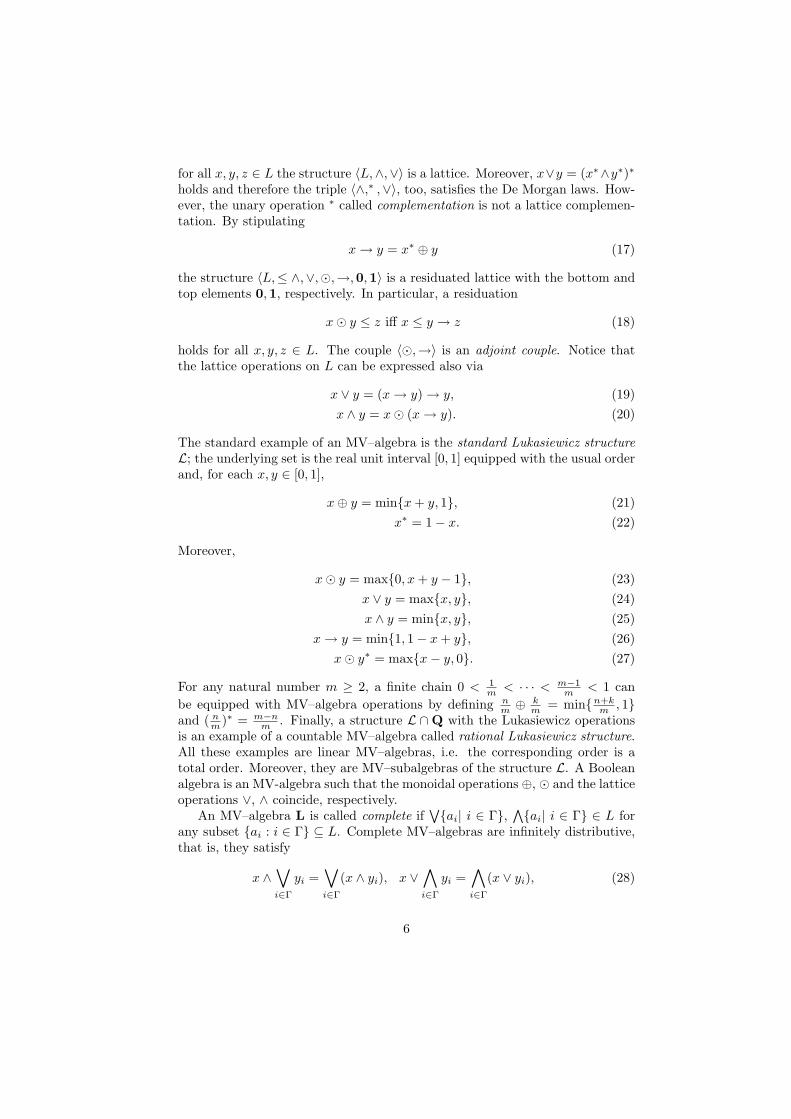
for all x, y, z ∈ L the structure 〈L,∧,∨〉 is a lattice. Moreover, x∨y = (x∗∧y∗)∗

holds and therefore the triple 〈∧,∗ ,∨〉, too, satisfies the De Morgan laws. How-ever, the unary operation ∗ called complementation is not a lattice complemen-tation. By stipulating

x → y = x∗ ⊕ y (17)

the structure 〈L,≤ ∧,∨,�,→,0,1〉 is a residuated lattice with the bottom andtop elements 0,1, respectively. In particular, a residuation

x� y ≤ z iff x ≤ y → z (18)

holds for all x, y, z ∈ L. The couple 〈�,→〉 is an adjoint couple. Notice thatthe lattice operations on L can be expressed also via

x ∨ y = (x → y) → y, (19)x ∧ y = x� (x → y). (20)

The standard example of an MV–algebra is the standard Lukasiewicz structureL; the underlying set is the real unit interval [0, 1] equipped with the usual orderand, for each x, y ∈ [0, 1],

x⊕ y = min{x + y, 1}, (21)x∗ = 1− x. (22)

Moreover,

x� y = max{0, x + y − 1}, (23)x ∨ y = max{x, y}, (24)x ∧ y = min{x, y}, (25)

x → y = min{1, 1− x + y}, (26)x� y∗ = max{x− y, 0}. (27)

For any natural number m ≥ 2, a finite chain 0 < 1m < · · · < m−1

m < 1 canbe equipped with MV–algebra operations by defining n

m ⊕ km = min{n+k

m , 1}and ( n

m )∗ = m−nm . Finally, a structure L ∩Q with the Lukasiewicz operations

is an example of a countable MV–algebra called rational Lukasiewicz structure.All these examples are linear MV–algebras, i.e. the corresponding order is atotal order. Moreover, they are MV–subalgebras of the structure L. A Booleanalgebra is an MV-algebra such that the monoidal operations ⊕, � and the latticeoperations ∨, ∧ coincide, respectively.

An MV–algebra L is called complete if∨{ai| i ∈ Γ},

∧{ai| i ∈ Γ} ∈ L for

any subset {ai : i ∈ Γ} ⊆ L. Complete MV–algebras are infinitely distributive,that is, they satisfy

x ∧∨i∈Γ

yi =∨i∈Γ

(x ∧ yi), x ∨∧i∈Γ

yi =∧i∈Γ

(x ∨ yi), (28)

6

for any x ∈ L, {yi| i ∈ Γ} ⊆ L. Thus, in a complete MV–algebra we can defineanother adjoint couple 〈∧,⇒〉, where the operation ⇒ is defined via

x ⇒ y =∨{z| x ∧ z ≤ y}. (29)

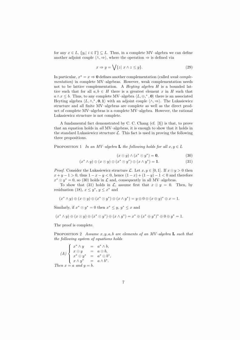
In particular, x? = x ⇒ 0 defines another complementation (called weak comple-mentation) in complete MV–algebras. However, weak complementation needsnot to be lattice complementation. A Heyting algebra H is a bounded lat-tice such that for all a, b ∈ H there is a greatest element x in H such thata∧ x ≤ b. Thus, to any complete MV–algebra 〈L,⊕,∗ ,0〉 there is an associatedHeyting algebra 〈L,∧,? ,0,1〉 with an adjoint couple 〈∧,⇒〉. The Lukasiewiczstructure and all finite MV–algebras are complete as well as the direct prod-uct of complete MV–algebras is a complete MV–algebra. However, the rationalLukasiewicz structure is not complete.

A fundamental fact demonstrated by C. C. Chang (cf. [3]) is that, to provethat an equation holds in all MV–algebras, it is enough to show that it holds inthe standard Lukasiewicz structure L. This fact is used in proving the followingthree propositions.

Proposition 1 In an MV–algebra L the following holds for all x, y ∈ L

(x� y) ∧ (x∗ � y∗) = 0, (30)(x∗ ∧ y)⊕ (x� y)⊕ (x∗ � y∗)⊕ (x ∧ y∗) = 1. (31)

Proof. Consider the Lukasiewicz structure L. Let x, y ∈ [0, 1]. If x� y > 0 thenx + y− 1 > 0, thus 1− x− y < 0, hence (1− x) + (1− y)− 1 < 0 and thereforex∗ � y∗ = 0, so (30) holds in L and, consequently in all MV–algebras.

To show that (31) holds in L, assume first that x � y = 0. Then, byresiduation (18), x ≤ y∗, y ≤ x∗ and

(x∗ ∧ y)⊕ (x� y)⊕ (x∗ � y∗)⊕ (x ∧ y∗) = y ⊕ 0⊕ (x⊕ y)∗ ⊕ x = 1.

Similarly, if x∗ � y∗ = 0 then x∗ ≤ y, y∗ ≤ x and

(x∗ ∧ y)⊕ (x� y)⊕ (x∗ � y∗)⊕ (x ∧ y∗) = x∗ ⊕ (x∗ ⊕ y∗)∗ ⊕ 0⊕ y∗ = 1.

The proof is complete.

Proposition 2 Assume x, y, a, b are elements of an MV–algebra L such thatthe following system of equations holds

(A)

x∗ ∧ y = a∗ ∧ b,x� y = a� b,x∗ � y∗ = a∗ � b∗,x ∧ y∗ = a ∧ b∗.

Then x = a and y = b.

7

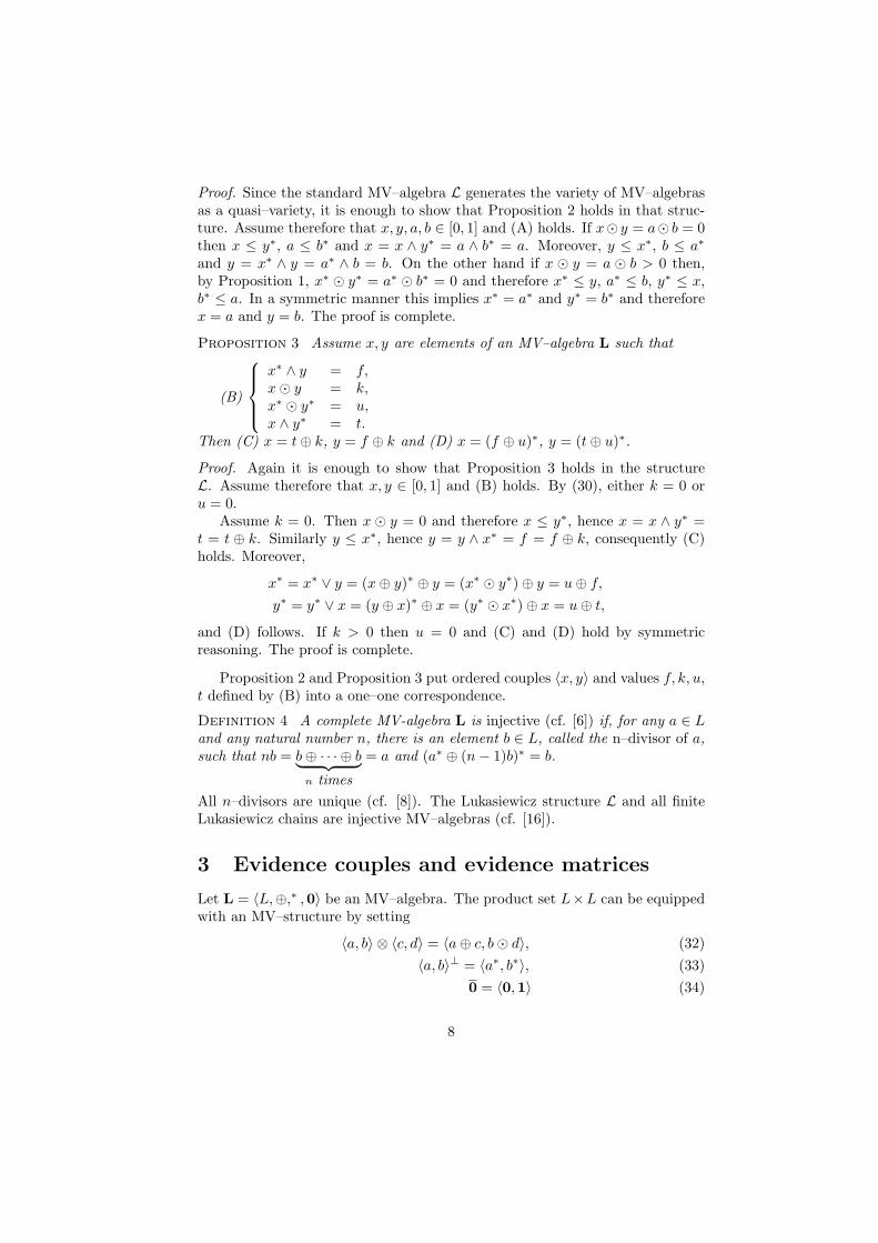
Proof. Since the standard MV–algebra L generates the variety of MV–algebrasas a quasi–variety, it is enough to show that Proposition 2 holds in that struc-ture. Assume therefore that x, y, a, b ∈ [0, 1] and (A) holds. If x� y = a� b = 0then x ≤ y∗, a ≤ b∗ and x = x ∧ y∗ = a ∧ b∗ = a. Moreover, y ≤ x∗, b ≤ a∗

and y = x∗ ∧ y = a∗ ∧ b = b. On the other hand if x � y = a � b > 0 then,by Proposition 1, x∗ � y∗ = a∗ � b∗ = 0 and therefore x∗ ≤ y, a∗ ≤ b, y∗ ≤ x,b∗ ≤ a. In a symmetric manner this implies x∗ = a∗ and y∗ = b∗ and thereforex = a and y = b. The proof is complete.

Proposition 3 Assume x, y are elements of an MV–algebra L such that

(B)

x∗ ∧ y = f,x� y = k,x∗ � y∗ = u,x ∧ y∗ = t.

Then (C) x = t⊕ k, y = f ⊕ k and (D) x = (f ⊕ u)∗, y = (t⊕ u)∗.

Proof. Again it is enough to show that Proposition 3 holds in the structureL. Assume therefore that x, y ∈ [0, 1] and (B) holds. By (30), either k = 0 oru = 0.

Assume k = 0. Then x � y = 0 and therefore x ≤ y∗, hence x = x ∧ y∗ =t = t ⊕ k. Similarly y ≤ x∗, hence y = y ∧ x∗ = f = f ⊕ k, consequently (C)holds. Moreover,

x∗ = x∗ ∨ y = (x⊕ y)∗ ⊕ y = (x∗ � y∗)⊕ y = u⊕ f,

y∗ = y∗ ∨ x = (y ⊕ x)∗ ⊕ x = (y∗ � x∗)⊕ x = u⊕ t,

and (D) follows. If k > 0 then u = 0 and (C) and (D) hold by symmetricreasoning. The proof is complete.

Proposition 2 and Proposition 3 put ordered couples 〈x, y〉 and values f, k, u,t defined by (B) into a one–one correspondence.

Definition 4 A complete MV-algebra L is injective (cf. [6]) if, for any a ∈ Land any natural number n, there is an element b ∈ L, called the n–divisor of a,such that nb = b⊕ · · · ⊕ b︸ ︷︷ ︸

n times

= a and (a∗ ⊕ (n− 1)b)∗ = b.

All n–divisors are unique (cf. [8]). The Lukasiewicz structure L and all finiteLukasiewicz chains are injective MV–algebras (cf. [16]).

3 Evidence couples and evidence matrices

Let L = 〈L,⊕,∗ ,0〉 be an MV–algebra. The product set L×L can be equippedwith an MV–structure by setting

〈a, b〉 ⊗ 〈c, d〉 = 〈a⊕ c, b� d〉, (32)〈a, b〉⊥ = 〈a∗, b∗〉, (33)

0 = 〈0,1〉 (34)

8

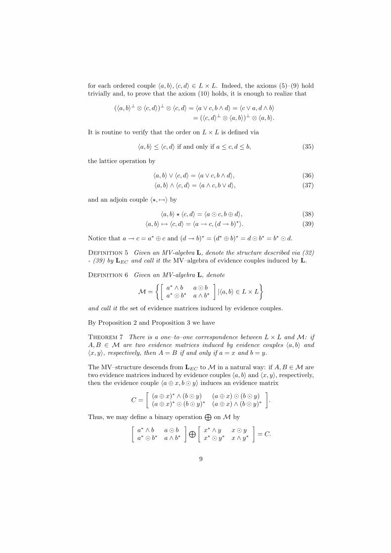
for each ordered couple 〈a, b〉, 〈c, d〉 ∈ L × L. Indeed, the axioms (5)–(9) holdtrivially and, to prove that the axiom (10) holds, it is enough to realize that

(〈a, b〉⊥ ⊗ 〈c, d〉)⊥ ⊗ 〈c, d〉 = 〈a ∨ c, b ∧ d〉 = 〈c ∨ a, d ∧ b〉= (〈c, d〉⊥ ⊗ 〈a, b〉)⊥ ⊗ 〈a, b〉.

It is routine to verify that the order on L× L is defined via

〈a, b〉 ≤ 〈c, d〉 if and only if a ≤ c, d ≤ b, (35)

the lattice operation by

〈a, b〉 ∨ 〈c, d〉 = 〈a ∨ c, b ∧ d〉, (36)〈a, b〉 ∧ 〈c, d〉 = 〈a ∧ c, b ∨ d〉, (37)

and an adjoin couple 〈?, 7→〉 by

〈a, b〉 ? 〈c, d〉 = 〈a� c, b⊕ d〉, (38)〈a, b〉 7→ 〈c, d〉 = 〈a → c, (d → b)∗〉. (39)

Notice that a → c = a∗ ⊕ c and (d → b)∗ = (d∗ ⊕ b)∗ = d� b∗ = b∗ � d.

Definition 5 Given an MV-algebra L, denote the structure described via (32)- (39) by LEC and call it the MV–algebra of evidence couples induced by L.

Definition 6 Given an MV-algebra L, denote

M ={[

a∗ ∧ b a� ba∗ � b∗ a ∧ b∗

]|〈a, b〉 ∈ L× L

}and call it the set of evidence matrices induced by evidence couples.

By Proposition 2 and Proposition 3 we have

Theorem 7 There is a one–to–one correspondence between L × L and M: ifA,B ∈ M are two evidence matrices induced by evidence couples 〈a, b〉 and〈x, y〉, respectively, then A = B if and only if a = x and b = y.

The MV–structure descends from LEC to M in a natural way: if A,B ∈M aretwo evidence matrices induced by evidence couples 〈a, b〉 and 〈x, y〉, respectively,then the evidence couple 〈a⊕ x, b� y〉 induces an evidence matrix

C =[

(a⊕ x)∗ ∧ (b� y) (a⊕ x)� (b� y)(a⊕ x)∗ � (b� y)∗ (a⊕ x) ∧ (b� y)∗

].

Thus, we may define a binary operation⊕

on M by[a∗ ∧ b a� ba∗ � b∗ a ∧ b∗

]⊕ [x∗ ∧ y x� yx∗ � y∗ x ∧ y∗

]= C.

9

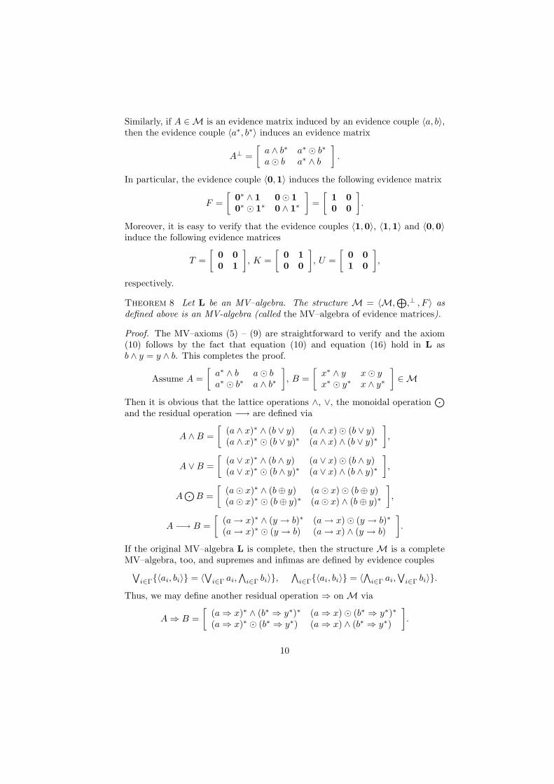
Similarly, if A ∈M is an evidence matrix induced by an evidence couple 〈a, b〉,then the evidence couple 〈a∗, b∗〉 induces an evidence matrix

A⊥ =[

a ∧ b∗ a∗ � b∗

a� b a∗ ∧ b

].

In particular, the evidence couple 〈0,1〉 induces the following evidence matrix

F =[

0∗ ∧ 1 0� 10∗ � 1∗ 0 ∧ 1∗

]=

[1 00 0

].

Moreover, it is easy to verify that the evidence couples 〈1,0〉, 〈1,1〉 and 〈0,0〉induce the following evidence matrices

T =[

0 00 1

], K =

[0 10 0

], U =

[0 01 0

],

respectively.

Theorem 8 Let L be an MV–algebra. The structure M = 〈M,⊕

,⊥ , F 〉 asdefined above is an MV-algebra (called the MV–algebra of evidence matrices).

Proof. The MV–axioms (5) – (9) are straightforward to verify and the axiom(10) follows by the fact that equation (10) and equation (16) hold in L asb ∧ y = y ∧ b. This completes the proof.

Assume A =[

a∗ ∧ b a� ba∗ � b∗ a ∧ b∗

], B =

[x∗ ∧ y x� yx∗ � y∗ x ∧ y∗

]∈M

Then it is obvious that the lattice operations ∧, ∨, the monoidal operation⊙

and the residual operation −→ are defined via

A ∧B =[

(a ∧ x)∗ ∧ (b ∨ y) (a ∧ x)� (b ∨ y)(a ∧ x)∗ � (b ∨ y)∗ (a ∧ x) ∧ (b ∨ y)∗

],

A ∨B =[

(a ∨ x)∗ ∧ (b ∧ y) (a ∨ x)� (b ∧ y)(a ∨ x)∗ � (b ∧ y)∗ (a ∨ x) ∧ (b ∧ y)∗

],

A⊙

B =[

(a� x)∗ ∧ (b⊕ y) (a� x)� (b⊕ y)(a� x)∗ � (b⊕ y)∗ (a� x) ∧ (b⊕ y)∗

],

A −→ B =[

(a → x)∗ ∧ (y → b)∗ (a → x)� (y → b)∗

(a → x)∗ � (y → b) (a → x) ∧ (y → b)

].

If the original MV–algebra L is complete, then the structure M is a completeMV–algebra, too, and supremes and infimas are defined by evidence couples∨

i∈Γ{〈ai, bi〉} = 〈∨

i∈Γ ai,∧

i∈Γ bi〉},∧

i∈Γ{〈ai, bi〉} = 〈∧

i∈Γ ai,∨

i∈Γ bi〉}.

Thus, we may define another residual operation ⇒ on M via

A ⇒ B =[

(a ⇒ x)∗ ∧ (b∗ ⇒ y∗)∗ (a ⇒ x)� (b∗ ⇒ y∗)∗

(a ⇒ x)∗ � (b∗ ⇒ y∗) (a ⇒ x) ∧ (b∗ ⇒ y∗)

].

10

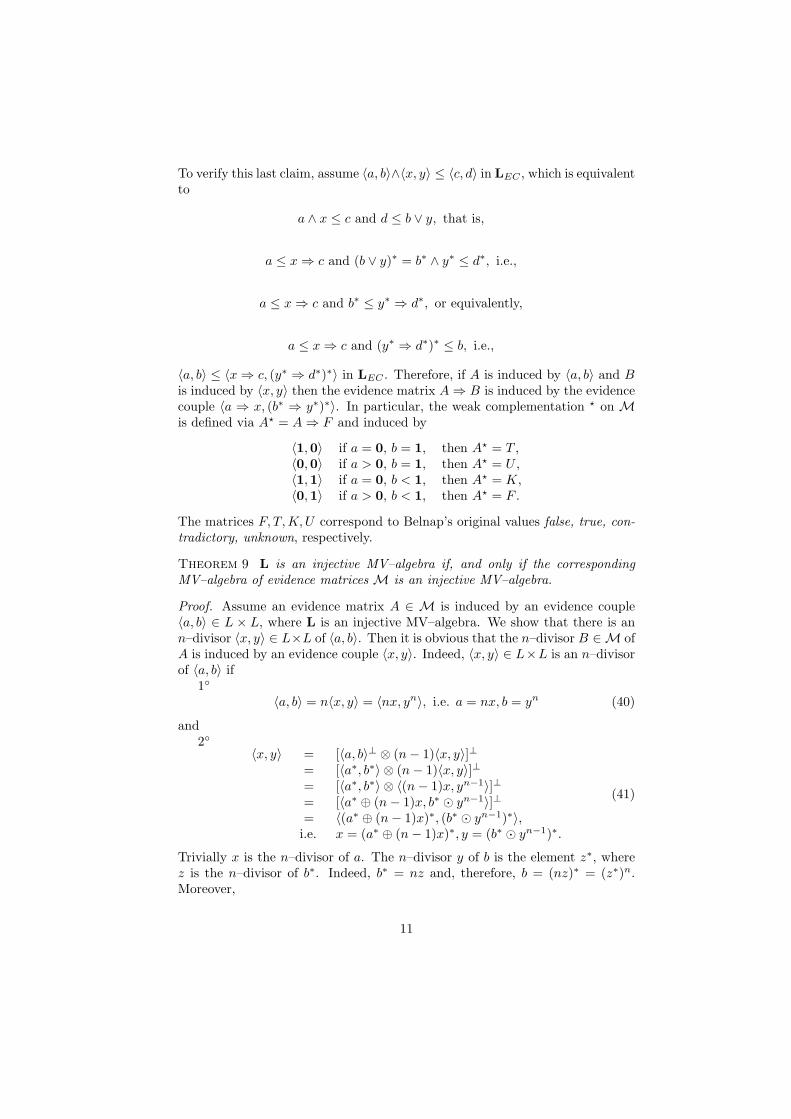
To verify this last claim, assume 〈a, b〉∧〈x, y〉 ≤ 〈c, d〉 in LEC , which is equivalentto

a ∧ x ≤ c and d ≤ b ∨ y, that is,

a ≤ x ⇒ c and (b ∨ y)∗ = b∗ ∧ y∗ ≤ d∗, i.e.,

a ≤ x ⇒ c and b∗ ≤ y∗ ⇒ d∗, or equivalently,

a ≤ x ⇒ c and (y∗ ⇒ d∗)∗ ≤ b, i.e.,

〈a, b〉 ≤ 〈x ⇒ c, (y∗ ⇒ d∗)∗〉 in LEC . Therefore, if A is induced by 〈a, b〉 and Bis induced by 〈x, y〉 then the evidence matrix A ⇒ B is induced by the evidencecouple 〈a ⇒ x, (b∗ ⇒ y∗)∗〉. In particular, the weak complementation ? on Mis defined via A? = A ⇒ F and induced by

〈1,0〉 if a = 0, b = 1, then A? = T ,〈0,0〉 if a > 0, b = 1, then A? = U ,〈1,1〉 if a = 0, b < 1, then A? = K,〈0,1〉 if a > 0, b < 1, then A? = F .

The matrices F, T,K,U correspond to Belnap’s original values false, true, con-tradictory, unknown, respectively.

Theorem 9 L is an injective MV–algebra if, and only if the correspondingMV–algebra of evidence matrices M is an injective MV–algebra.

Proof. Assume an evidence matrix A ∈ M is induced by an evidence couple〈a, b〉 ∈ L × L, where L is an injective MV–algebra. We show that there is ann–divisor 〈x, y〉 ∈ L×L of 〈a, b〉. Then it is obvious that the n–divisor B ∈M ofA is induced by an evidence couple 〈x, y〉. Indeed, 〈x, y〉 ∈ L×L is an n–divisorof 〈a, b〉 if

1◦

〈a, b〉 = n〈x, y〉 = 〈nx, yn〉, i.e. a = nx, b = yn (40)

and2◦

〈x, y〉 = [〈a, b〉⊥ ⊗ (n− 1)〈x, y〉]⊥= [〈a∗, b∗〉 ⊗ (n− 1)〈x, y〉]⊥= [〈a∗, b∗〉 ⊗ 〈(n− 1)x, yn−1〉]⊥= [〈a∗ ⊕ (n− 1)x, b∗ � yn−1〉]⊥= 〈(a∗ ⊕ (n− 1)x)∗, (b∗ � yn−1)∗〉,i.e. x = (a∗ ⊕ (n− 1)x)∗, y = (b∗ � yn−1)∗.

(41)

Trivially x is the n–divisor of a. The n–divisor y of b is the element z∗, wherez is the n–divisor of b∗. Indeed, b∗ = nz and, therefore, b = (nz)∗ = (z∗)n.Moreover,

11

z = [b∗∗ ⊕ (n− 1)z]∗ = [b⊕ (n− 1)z]∗ = b∗ � [(n− 1)z]∗ = b∗ � (z∗)n−1,

hence z∗ = [b∗ � (z∗)n−1]∗. By the above construction we also see that if M isan injective MV–algebra, then L is an injective, too. This completes the proof.

Remark 10 Some of the proofs in this section would be shorter after realizingthat the structure introduced in Definition 5 is, up to isomorphism, the wellknown MV–algebra L × Ldual, where Ldual is obtained by reversing the order.For the convenience of those readers who are not familiar with MV–algebras wehave, however, presented some proofs in detail.

4 Paraconsistent Pavelka style fuzzy logic

Now we briefly demonstrate Pavelka style fuzzy logic with above introducedparaconsistent semantics. For a complete description of injective MV–algebravalued Pavelka style sentential logic, see [16].

4.1 Pavelka style fuzzy logic

A standard approach in mathematical sentential logic is the following. Afterintroducing atomic formulae, logical connectives and the set of well–formed for-mulae, these formulae are semantically interpreted in suitable algebraic struc-tures. In Classical logic these structures are Boolean algebras, in Hajek’s Basicfuzzy logic [7], for example, the suitable structures are standard BL–algebras.Tautologies of a logic are those formulae that obtain the top value 1 in all in-terpretations in all suitable algebraic structures; for this reason tautologies aresometimes called 1-tautologies. For example, tautologies in Basic fuzzy logic areexactly the formulae that obtain value 1 in all interpretations in all standardBL–algebras. Next step in usual mathematical logic is to fix the axiom schemeand the rules of inference: a well–formed formula is a theorem if it is eitheran axiom or obtained recursively from axioms by using finite many times rulesof inference. Completeness of the logic means that tautologies and theoremscoincide; Classical sentential logic and Basic fuzzy sentential logic, for example,are complete logics.

In Pavelka style fuzzy sentential logic [11] the situation is somewhat different.We start by fixing a set of truth values, in fact an algebraic structure – inPavelka’s own approach this structure is the Lukasiewicz structure L – in [15, 16]the structure is a more general (but fixed!) injective MV–algebra L.

Consider a zero order language F with a set of infinite many propositionalvariables p, q, r, · · · , and a set of internal truth values {a | a ∈ L} (also calledtruth constants ) corresponding to the elements in the set L. Proved in [7], ifthe set of truth values is the whole real interval [0, 1] then it is enough to includeinner truth values corresponding to rationales belonging to [0, 1]. In two–valuedlogic inner truth values correspond to the truth constants ⊥ and >. Thesetwo sets of objects constitute the set Fa of atomic formulae. The elementarylogical connectives are implication ’imp’ and conjunction ’and’. The set of all

12

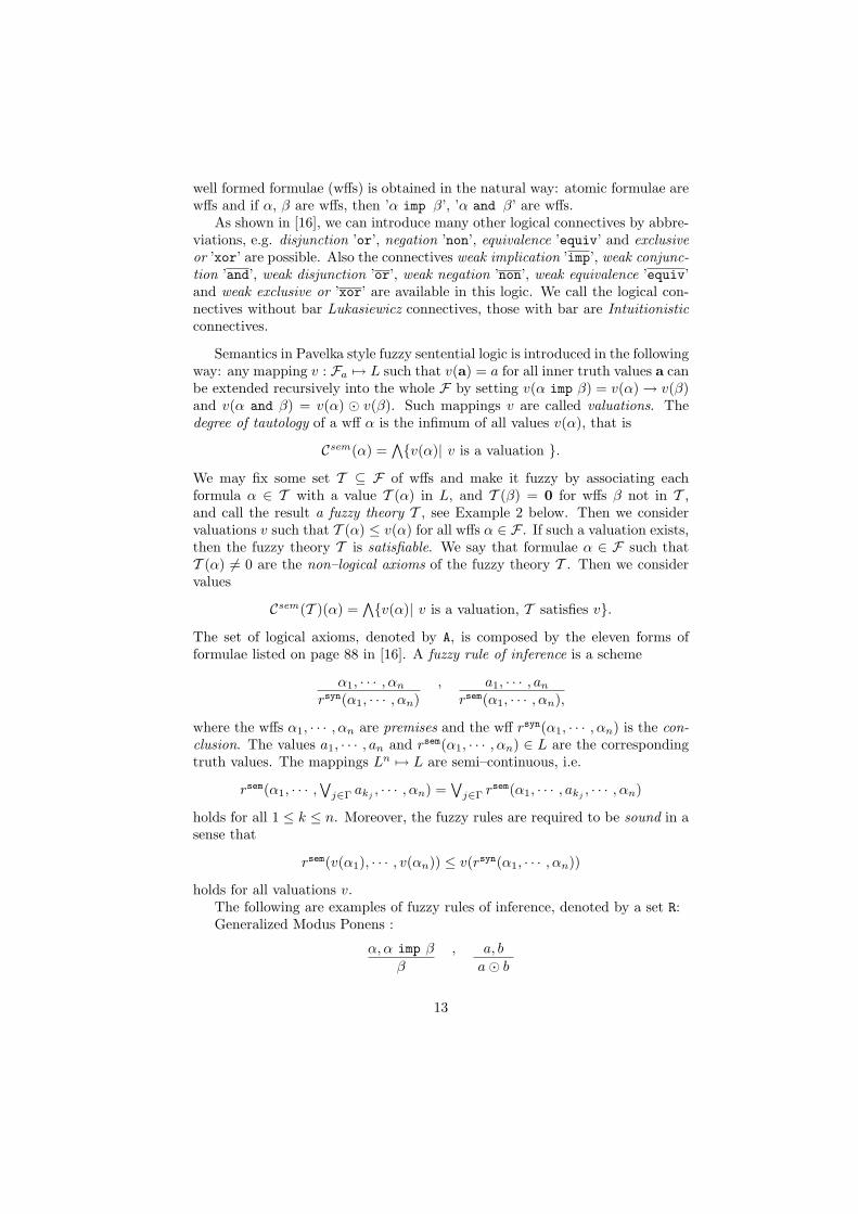
well formed formulae (wffs) is obtained in the natural way: atomic formulae arewffs and if α, β are wffs, then ’α imp β’, ’α and β’ are wffs.

As shown in [16], we can introduce many other logical connectives by abbre-viations, e.g. disjunction ’or’, negation ’non’, equivalence ’equiv’ and exclusiveor ’xor’ are possible. Also the connectives weak implication ’imp’, weak conjunc-tion ’and’, weak disjunction ’or’, weak negation ’non’, weak equivalence ’equiv’and weak exclusive or ’xor’ are available in this logic. We call the logical con-nectives without bar Lukasiewicz connectives, those with bar are Intuitionisticconnectives.

Semantics in Pavelka style fuzzy sentential logic is introduced in the followingway: any mapping v : Fa 7→ L such that v(a) = a for all inner truth values a canbe extended recursively into the whole F by setting v(α imp β) = v(α) → v(β)and v(α and β) = v(α) � v(β). Such mappings v are called valuations. Thedegree of tautology of a wff α is the infimum of all values v(α), that is

Csem(α) =∧{v(α)| v is a valuation }.

We may fix some set T ⊆ F of wffs and make it fuzzy by associating eachformula α ∈ T with a value T (α) in L, and T (β) = 0 for wffs β not in T ,and call the result a fuzzy theory T , see Example 2 below. Then we considervaluations v such that T (α) ≤ v(α) for all wffs α ∈ F . If such a valuation exists,then the fuzzy theory T is satisfiable. We say that formulae α ∈ F such thatT (α) 6= 0 are the non–logical axioms of the fuzzy theory T . Then we considervalues

Csem(T )(α) =∧{v(α)| v is a valuation, T satisfies v}.

The set of logical axioms, denoted by A, is composed by the eleven forms offormulae listed on page 88 in [16]. A fuzzy rule of inference is a scheme

α1, · · · , αn , a1, · · · , an

rsyn(α1, · · · , αn) rsem(α1, · · · , αn),

where the wffs α1, · · · , αn are premises and the wff rsyn(α1, · · · , αn) is the con-clusion. The values a1, · · · , an and rsem(α1, · · · , αn) ∈ L are the correspondingtruth values. The mappings Ln 7→ L are semi–continuous, i.e.

rsem(α1, · · · ,∨

j∈Γ akj, · · · , αn) =

∨j∈Γ rsem(α1, · · · , akj

, · · · , αn)

holds for all 1 ≤ k ≤ n. Moreover, the fuzzy rules are required to be sound in asense that

rsem(v(α1), · · · , v(αn)) ≤ v(rsyn(α1, · · · , αn))

holds for all valuations v.The following are examples of fuzzy rules of inference, denoted by a set R:Generalized Modus Ponens :

α, α imp β , a, b

β a� b

13

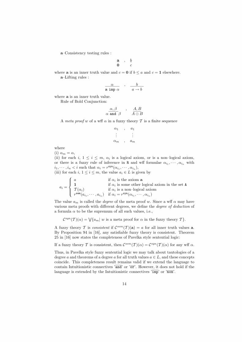
a–Consistency testing rules :

a , b0 c

where a is an inner truth value and c = 0 if b ≤ a and c = 1 elsewhere.a–Lifting rules :

α , ba imp α a → b

where a is an inner truth value.Rule of Bold Conjunction:

α, β , A,Bα and β A�B

A meta proof w of a wff α in a fuzzy theory T is a finite sequence

α1 , a1

......

αm , am

where(i) αm = α,(ii) for each i, 1 ≤ i ≤ m, αi is a logical axiom, or is a non–logical axiom,or there is a fuzzy rule of inference in R and wff formulae αi1 , · · · , αin withi1, · · · , in < i such that αi = rsyn(αi1 , · · · , αin

),(iii) for each i, 1 ≤ i ≤ m, the value ai ∈ L is given by

ai =

a if αi is the axiom a1 if αi is some other logical axiom in the set AT (αi) if αi is a non–logical axiomrsem(ai1 , · · · , ain

) if αi = rsyn(αi1 , · · · , αin)

The value am is called the degree of the meta proof w. Since a wff α may havevarious meta proofs with different degrees, we define the degree of deduction ofa formula α to be the supremum of all such values, i.e.,

Csyn(T )(α) =∨{am| w is a meta proof for α in the fuzzy theory T }.

A fuzzy theory T is consistent if Csem(T )(a) = a for all inner truth values a.By Proposition 94 in [16], any satisfiable fuzzy theory is consistent. Theorem25 in [16] now states the completeness of Pavelka style sentential logic:

If a fuzzy theory T is consistent, then Csem(T )(α) = Csyn(T )(α) for any wff α.

Thus, in Pavelka style fuzzy sentential logic we may talk about tautologies of adegree a and theorems of a degree a for all truth values a ∈ L, and these conceptscoincide. This completeness result remains valid if we extend the language tocontain Intuitionistic connectives ’and’ or ’or’. However, it does not hold if thelanguage is extended by the Intuitionistic connectives ’imp’ or ’non’.

14

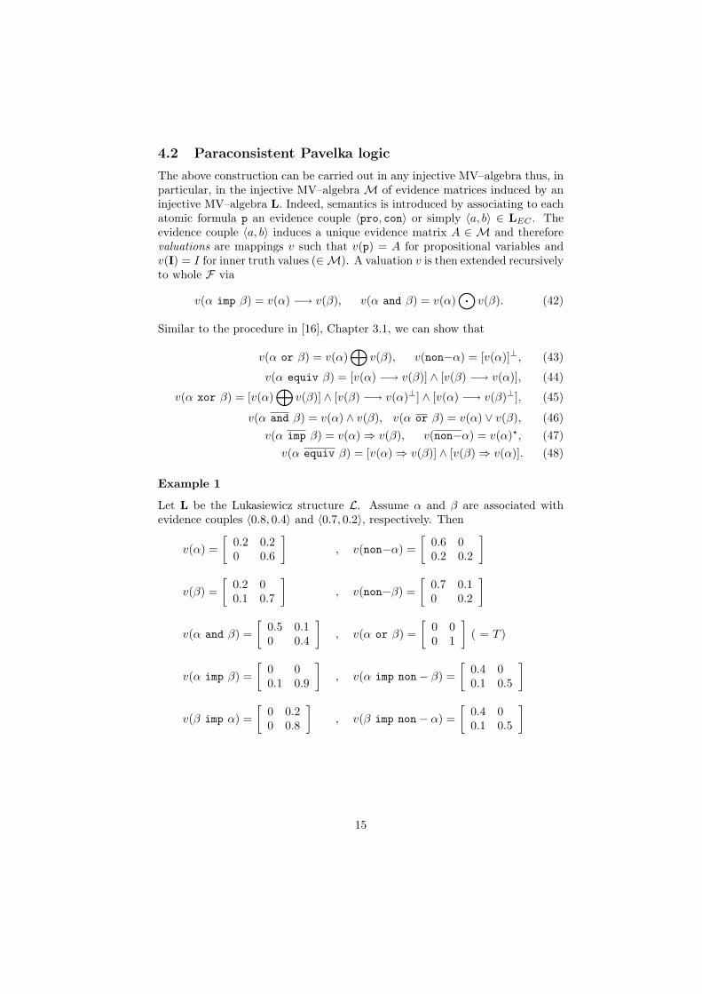
4.2 Paraconsistent Pavelka logic

The above construction can be carried out in any injective MV–algebra thus, inparticular, in the injective MV–algebra M of evidence matrices induced by aninjective MV–algebra L. Indeed, semantics is introduced by associating to eachatomic formula p an evidence couple 〈pro, con〉 or simply 〈a, b〉 ∈ LEC . Theevidence couple 〈a, b〉 induces a unique evidence matrix A ∈ M and thereforevaluations are mappings v such that v(p) = A for propositional variables andv(I) = I for inner truth values (∈M). A valuation v is then extended recursivelyto whole F via

v(α imp β) = v(α) −→ v(β), v(α and β) = v(α)⊙

v(β). (42)

Similar to the procedure in [16], Chapter 3.1, we can show that

v(α or β) = v(α)⊕

v(β), v(non−α) = [v(α)]⊥, (43)

v(α equiv β) = [v(α) −→ v(β)] ∧ [v(β) −→ v(α)], (44)

v(α xor β) = [v(α)⊕

v(β)] ∧ [v(β) −→ v(α)⊥] ∧ [v(α) −→ v(β)⊥], (45)

v(α and β) = v(α) ∧ v(β), v(α or β) = v(α) ∨ v(β), (46)v(α imp β) = v(α) ⇒ v(β), v(non−α) = v(α)?, (47)

v(α equiv β) = [v(α) ⇒ v(β)] ∧ [v(β) ⇒ v(α)]. (48)

Example 1

Let L be the Lukasiewicz structure L. Assume α and β are associated withevidence couples 〈0.8, 0.4〉 and 〈0.7, 0.2〉, respectively. Then

v(α) =[

0.2 0.20 0.6

], v(non−α) =

[0.6 00.2 0.2

]

v(β) =[

0.2 00.1 0.7

], v(non−β) =

[0.7 0.10 0.2

]

v(α and β) =[

0.5 0.10 0.4

], v(α or β) =

[0 00 1

]( = T )

v(α imp β) =[

0 00.1 0.9

], v(α imp non− β) =

[0.4 00.1 0.5

]

v(β imp α) =[

0 0.20 0.8

], v(β imp non− α) =

[0.4 00.1 0.5

]

15

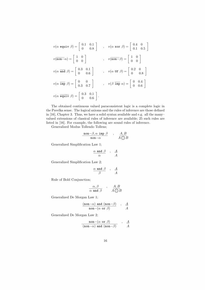
v(α equiv β) =[

0.1 0.10 0.8

], v(α xor β) =

[0.4 00.1 0.5

]

v(non−α) =[

1 00 0

], v(non−β) =

[1 00 0

]

v(α and β) =[

0.3 0.10 0.6

], v(α or β) =

[0.2 00 0.8

]

v(α imp β) =[

0 00.3 0.7

], v(β imp α) =

[0 0.40 0.6

]

v(α equiv β) =[

0.3 0.10 0.6

].

The obtained continuous valued paraconsistent logic is a complete logic inthe Pavelka sense. The logical axioms and the rules of inference are those definedin [16], Chapter 3. Thus, we have a solid syntax available and e.g. all the many–valued extensions of classical rules of inference are available; 25 such rules arelisted in [16]. For example, the following are sound rules of inference.

Generalized Modus Tollendo Tollens;

non−β, α imp β , A,B

non−α A⊙

B

Generalized Simplification Law 1;

α and β , Aα A

Generalized Simplification Law 2;

α and β , Aβ A

Rule of Bold Conjunction;

α, β , A,Bα and β A

⊙B

Generalized De Morgan Law 1;

(non−α) and (non−β) , A

non−(α or β) A

Generalized De Morgan Law 2;

non−(α or β) , A

(non−α) and (non−β) A

16

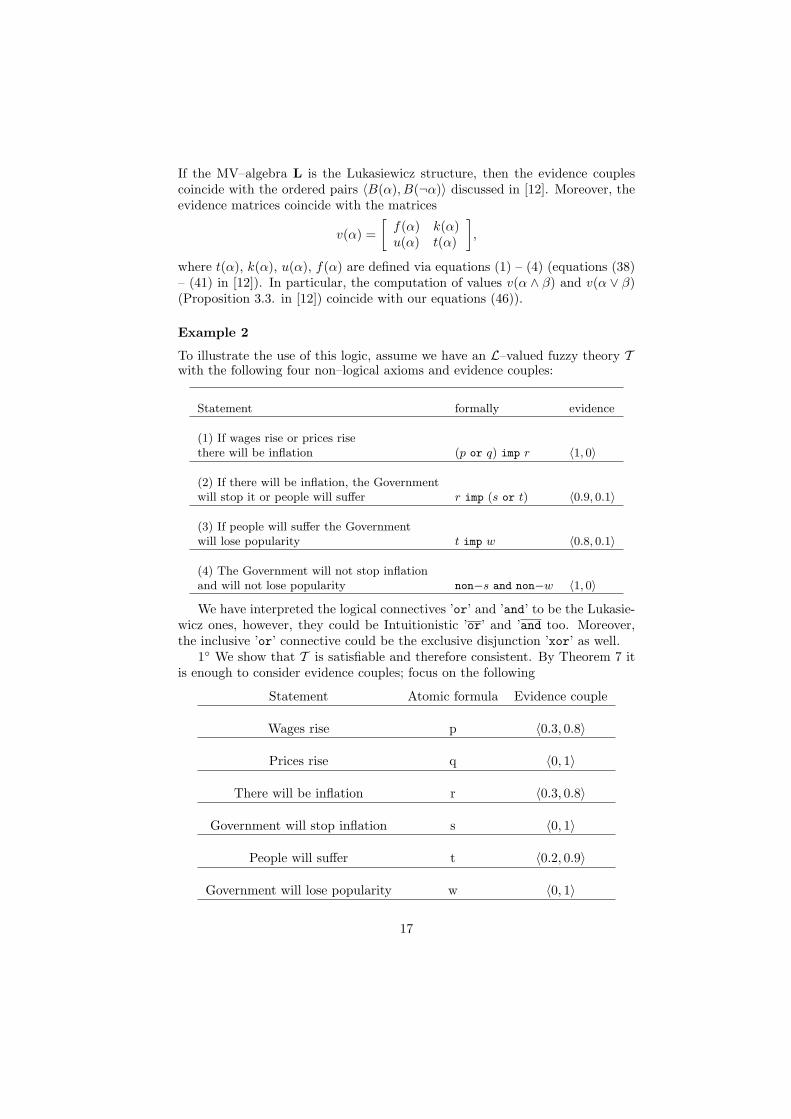
If the MV–algebra L is the Lukasiewicz structure, then the evidence couplescoincide with the ordered pairs 〈B(α), B(¬α)〉 discussed in [12]. Moreover, theevidence matrices coincide with the matrices

v(α) =[

f(α) k(α)u(α) t(α)

],

where t(α), k(α), u(α), f(α) are defined via equations (1) – (4) (equations (38)– (41) in [12]). In particular, the computation of values v(α ∧ β) and v(α ∨ β)(Proposition 3.3. in [12]) coincide with our equations (46)).

Example 2

To illustrate the use of this logic, assume we have an L–valued fuzzy theory Twith the following four non–logical axioms and evidence couples:

Statement formally evidence

(1) If wages rise or prices risethere will be inflation (p or q) imp r 〈1, 0〉

(2) If there will be inflation, the Governmentwill stop it or people will suffer r imp (s or t) 〈0.9, 0.1〉

(3) If people will suffer the Governmentwill lose popularity t imp w 〈0.8, 0.1〉

(4) The Government will not stop inflationand will not lose popularity non−s and non−w 〈1, 0〉

We have interpreted the logical connectives ’or’ and ’and’ to be the Lukasie-wicz ones, however, they could be Intuitionistic ’or’ and ’and too. Moreover,the inclusive ’or’ connective could be the exclusive disjunction ’xor’ as well.

1◦ We show that T is satisfiable and therefore consistent. By Theorem 7 itis enough to consider evidence couples; focus on the following

Statement Atomic formula Evidence couple

Wages rise p 〈0.3, 0.8〉

Prices rise q 〈0, 1〉

There will be inflation r 〈0.3, 0.8〉

Government will stop inflation s 〈0, 1〉

People will suffer t 〈0.2, 0.9〉

Government will lose popularity w 〈0, 1〉

17

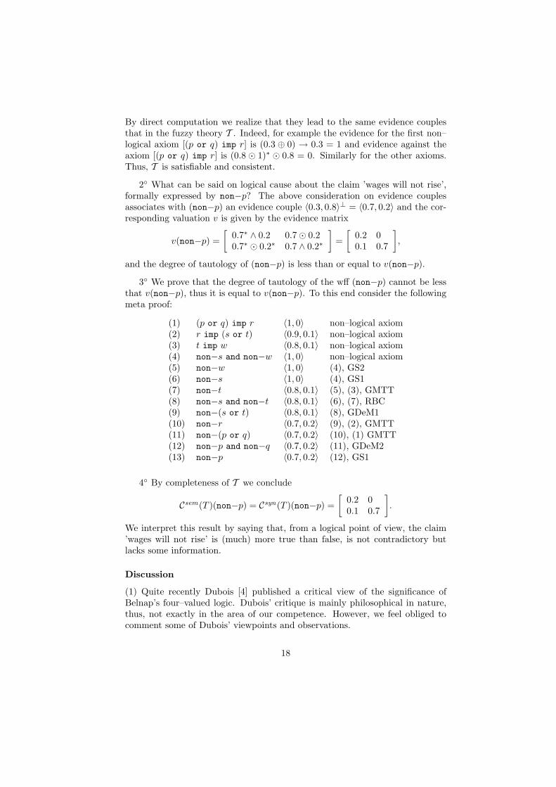
By direct computation we realize that they lead to the same evidence couplesthat in the fuzzy theory T . Indeed, for example the evidence for the first non–logical axiom [(p or q) imp r] is (0.3 ⊕ 0) → 0.3 = 1 and evidence against theaxiom [(p or q) imp r] is (0.8 � 1)∗ � 0.8 = 0. Similarly for the other axioms.Thus, T is satisfiable and consistent.

2◦ What can be said on logical cause about the claim ’wages will not rise’,formally expressed by non−p? The above consideration on evidence couplesassociates with (non−p) an evidence couple 〈0.3, 0.8〉⊥ = 〈0.7, 0.2〉 and the cor-responding valuation v is given by the evidence matrix

v(non−p) =[

0.7∗ ∧ 0.2 0.7� 0.20.7∗ � 0.2∗ 0.7 ∧ 0.2∗

]=

[0.2 00.1 0.7

],

and the degree of tautology of (non−p) is less than or equal to v(non−p).

3◦ We prove that the degree of tautology of the wff (non−p) cannot be lessthat v(non−p), thus it is equal to v(non−p). To this end consider the followingmeta proof:

(1) (p or q) imp r 〈1, 0〉 non–logical axiom(2) r imp (s or t) 〈0.9, 0.1〉 non–logical axiom(3) t imp w 〈0.8, 0.1〉 non–logical axiom(4) non−s and non−w 〈1, 0〉 non–logical axiom(5) non−w 〈1, 0〉 (4), GS2(6) non−s 〈1, 0〉 (4), GS1(7) non−t 〈0.8, 0.1〉 (5), (3), GMTT(8) non−s and non−t 〈0.8, 0.1〉 (6), (7), RBC(9) non−(s or t) 〈0.8, 0.1〉 (8), GDeM1(10) non−r 〈0.7, 0.2〉 (9), (2), GMTT(11) non−(p or q) 〈0.7, 0.2〉 (10), (1) GMTT(12) non−p and non−q 〈0.7, 0.2〉 (11), GDeM2(13) non−p 〈0.7, 0.2〉 (12), GS1

4◦ By completeness of T we conclude

Csem(T )(non−p) = Csyn(T )(non−p) =[

0.2 00.1 0.7

].

We interpret this result by saying that, from a logical point of view, the claim’wages will not rise’ is (much) more true than false, is not contradictory butlacks some information.

Discussion

(1) Quite recently Dubois [4] published a critical view of the significance ofBelnap’s four–valued logic. Dubois’ critique is mainly philosophical in nature,thus, not exactly in the area of our competence. However, we feel obliged tocomment some of Dubois’ viewpoints and observations.

18

Dubois writes ’Although some may be tempted to found new mathematics onmany–valued logics, this grand purpose still looks out of reach if not delusive. Itsound like a paradox of its own since we use classical mathematics to formallymodel many–valued logic notations.’ We share this criticism. For us variousmany–valued logics are just formal mathematical systems whose meta logic isclassical Boolean logic. For example the Completeness Theorem of Pavelka logichas exactly the same status than Central Limit Theorem has in probabilitytheory; there is no uncertainty or many–valuedness involved, they are mattersof exact proof.

Moreover, Dubois discusses meritoriously about the philosophical differencesbetween truth and belief and points out that there is a confusion in the use ofthese concepts in Belnap’s approach. We feel that this critique does not concernour approach as for us the introduced continuous valued logic is just a formaltool mainly developed for decision making purposes and, hence, without anycontentions on the philosophy of science. Indeed, given an evidence couple, wemay interpret the values t, f, k and u of the corresponding evidence matrixM e.g. by Make the resolution, Do not make the resolution, Information iscontradictory and There is a lack of information, respectively. In general, we donot care if the four values ultimately represent truth. We have a language whichmaps sentences to four possible states (or the infinite combinations betweenthem) and we show how is it possible to make a consistent calculus on that. Ifsuch states represent information or belief states we simply do not care.

Finally, Dubois observes an anomaly in Belnap’s approach as

(α and β) or (not−α and β) or (α and not−β) or (not−α and not−β) (49)

is not a tautology but obtains the same value of truth than F (false). This isdue to the fact that, in Belnap’s approach, the negation of U (unknown) is Uand the negation of K (contradiction) is K. Our approach avoids this pitfall aswe use residual negation. Indeed, as one can easily be convinced, (49) obtainsthe top value 1 in any valuation v.

(2) Assuming L is a linearly ordered injective MV–algebra, the condition(B) in Proposition 3 implies that, for any formula α, either k has the bottomvalue 0 or u has the bottom value, which might sound counter intuitive. If kand u represent information or epistemic states this is, however, not surprising.Intuitively speaking we either have a situation of information overload (contra-diction) or of missing information (unknown), but never both. However, theremight be situations where there is not enough information and even the existingpiece of information contains contradictions. In such cases we simply assumethat L is not linear as, in general, k∧u = 0 does not imply that k = 0 or u = 0.

(3) As a possible direction of future work we mention a more detailed discus-sion about the resolution of the problems encountered in [12] as well as a moredetailed presentation of the relevance of all that for preference modeling anddecision making purposes. Last, but not least we mention possible links withargumentation theory which explicitly considers positive and negative reasonsfor reaching a conclusion.

19

Acknowledgement This paper is part of research project COST ActionI0602 Algorithmic Decision Theory. The authors are grateful to Rostislav Horcıkfor his valuable comments when preparing the paper.

References

[1] O. Arieli, O. and Avron, A.: Reasoning with logical bilattices. Journal ofLogic, Language and Information, 5(1996), 25 – 63, .

[2] Belnap, N.D.: A useful four–valued logic, in Epstein, G. and Dumme, J.(eds.) Modern uses of multiple valued logics. D. Reidel, Dordrecht (1977), 8– 37.

[3] Chang, C. C. : Algebraic analysis of many-valued logics. Transactions of theAmerican Mathematical Society 88(1958), 476 – 90.

[4] Dubois, D. : On Ignorance and Contradiction Considered as Truth-values.Logic Journal of IGPL 16(2)(2008), 195 – 216.

[5] Ginsberg, M. K.: Multivalued Logics: A Uniform Approach to Inference inArtificial Intelligence. Computational Intelligence, 4 (1988), 265 – 316.

[6] Gluschankof, D.: Prime deductive systems and injective objects in the al-gebras of Lukasiewicz infinite–valued calculi. Algebra Universalis 29(1992),354 – 377.

[7] Hajek, P.: Metamathematics of Fuzzy Logic, Kluwer (1998).

[8] Kukkurainen, P. and Turunen, E.: Many-valued Similarity Reasoning.An Axiomatic Approach. International Journal of Multiple Valued Logic8(2002), 751 – 760.

[9] Cignoli, R., D’Ottaviano I.M.L. and Mundici, D.: Algebraic Foundations ofmany-valued Reasoning, Trends in Logic, vol. 7, Kluwer Academic Publish-ers, Dordrecht, 2000.

[10] Novak, V., Perfilieva, I., Mockor, J.: Mathematical Principles of FuzzyLogic, Kluwer, Boston, 1999.

[11] Pavelka, J.: On fuzzy logic I, II, III. Zeitsch. f. Math. Logik 25 (1979),45–52, 119–134, 447–464.

[12] Perny, P. and Tsoukias, A.: On the continuous extensions of four valuedlogic for preference modeling. Proceedings of the IPMU conference (1998),302 – 309.

[13] http://plato.stanford.edu/entries/logic-paraconsistent/

20

[14] Tsoukias, A.: A first order, four valued, weakly Paraconsistent logic andits relation to rough sets semantics. Foundations of Computing and DecisionSciences 12 (2002), 85 – 108.

[15] Turunen, E.: Well-defined Fuzzy Sentential Logic, Mathematical LogicQuarterly 41(1995), 236-248.

[16] Turunen, E.: Mathematics behind Fuzzy Logic. Springer–Verlag (1999).

[17] Turunen, E.: Interpreting GUHA Data Mining Logic in ParaconsistentFuzzy Logic Framework (submitted).

[18] 0zturk M., and Tsoukias A.: Modeling uncertain positive and negativereasons in decision aiding. Decision Support Systems 43(2007), 1512 – 1526.

21