paradata within the total survey error framework … (jpsm & iab/lmu) paradata fedcasic 2 / 14....

Paradata within the Total Survey Error FrameworkSuccesses, Challenges, and Gaps

Frauke Kreuter

Federal Computer-Assisted Survey Information Collection (FedCASIC) Workshop

March 27, 2012

Summary

We have seen successful uses of paradata togain efficiency, and toalert for errors.We face serious challenges to expand theconcurrent analytic use of paradata, thetailored collection of paradata, and the transferacross modes, surveys, and survey organizations.We might benefit from widening the scope toother error sources,through linkage with cost data and others,and from the use of paradata in modelling.

Kreuter (JPSM & IAB/LMU) Paradata FedCASIC 2 / 14

Outline . . .

1 Current Activities and Typical Applications

2 Challenges in Collection, Analysis, and Communication

3 Paradata inside the Total Survey Error Framework


Activities & Applications

Outline






Prevalent Paradata in TSE Framework Groves et al. 2004

Survey Statistic

prwy

Contact Data & Observations:

Day/Time; Result

Keys & Key Strokes: Missing data,

Response Times

Measurement

Postsurvey Adjustment

rwy

Target Population

Y

Sampling Frame

Cy

Sample

sy

Respondents

ry

Representation

Coverage Error

Sampling Error

Nonresponse Error

Adjustment Error

Construct

iμ

Measurement

iY

Response

iy

Edited Response

ipy

Validity

Processing Error

Measurement Error



Response Time

Substantive UseAttitudes as object-evaluation modelFazio et al. 1986, Dovidio & Fazio 1992.

Post-hoc Use - Focus on ErrorCharacteristics of Instrument and Setting:(+) poor wording, poor layout, length, complexity(-) logical order, practice, correct answers, decreasing motivatione.g. Bassili 1996, Draisma & Dijkstra 2004, Tourangeau, Couper & Conrad 2004, Yan & Tourangeau 2008

Interview administratione.g. Olson & Peytchev 2007, Couper & Kreuter 2012, Schafer 2012

Interview falsificationClements 2001; Penne, Snodgrass & Baker 2002

Concurrent Use - Focus on ErrorIntervention if respondents answer too fast Conrad et al. 2009

or too slow Conrad, Schober & Coiner 2007



Call record data

Post-hoc Use - Focus on EfficiencyOptimal call schedules Example

e.g. Weeks et al. 1980, Greenberg & Stokes 1990, Bates 2003, Laflamme 2008, Durrant et al. 2010

Predictors of response e.g. Campanelli et al. 1997, Groves & Couper 1998, Lynn 2003, Bates &

Piani 2005, Bates et al. 2008, Durrant & Steele 2009

Concurrent Use - Focus on EfficiencyCall scheduling (CATI)Monitoring Example

Post-hoc Use - Focus on ErrorNonresponse bias analyses Example

e.g. FedStat Surveys - since OMB Standard and Guidelines 2006

Nonresponse bias adjustment Politz & Simmons 1949, Kalton 1983, Beaumont 2005,

Biemer & Link 2006

Concurrent Use - Focus on ErrorInterventions Example


Challenges

Outline





Challenges

Now one could ask:

Why do we not see more research on key stroke data?⇒

Why do analysts struggle with f2f contact protocol data?⇒

Why do FRs shy away from call record protocols?⇒

Why are interviewer observations not used for adjustment?⇒

Why are adjusters disappointed about interviewer observations?⇒


Challenges

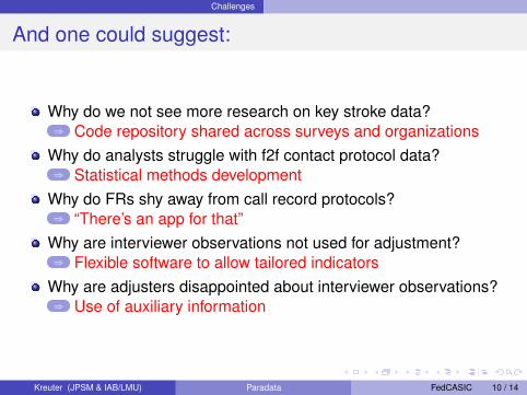
And one could suggest:

Why do we not see more research on key stroke data?⇒ Code repository shared across surveys and organizations

Why do analysts struggle with f2f contact protocol data?⇒ Statistical methods development

Why do FRs shy away from call record protocols?⇒ “There’s an app for that”

Why are interviewer observations not used for adjustment?⇒ Flexible software to allow tailored indicators

Why are adjusters disappointed about interviewer observations?⇒ Use of auxiliary information


TSE Framework

Outline





TSE Framework

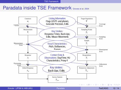
Paradata inside TSE Framework Groves et al. 2004

Survey Statistic

prwy

Listing Information: Flags (USPS and phone), Geocode Precision, Edits

Vocal Characteristics: Pitch, Disfluencies,

Pauses

Contact Data & Observations: Day/Time; HU

Characteristics; Proxy-Y

Key Strokes: Response Times; Back-Ups;

Edits; Mouse Movements

Construct

iμ

Measurement

iY

Response

iy

Edited Response

ipy

Sampling Error

Nonresponse Error

Adjustment Error

Postsurvey Adjustment

rwy

Target Population

Y

Sampling Frame

Cy

Sample

sy

Respondents

ry

Measurement Representation

Key strokes: Back-Ups; Edits

Coverage Error Validity

Measurement Error

Processing Error


TSE Framework

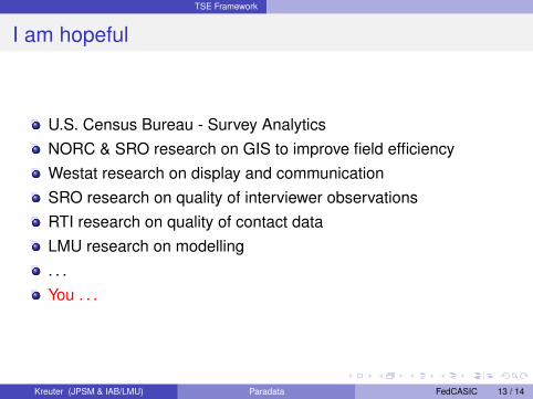
I am hopeful

U.S. Census Bureau - Survey AnalyticsNORC & SRO research on GIS to improve field efficiencyWestat research on display and communicationSRO research on quality of interviewer observationsRTI research on quality of contact dataLMU research on modelling. . .You . . .


TSE Framework

Thank You!

[email protected]


Contact Rates by Hour and Day in NSFG Wagner 2012

5

The result of each call (�� 1 for contact and 0 for no contact for the ith person on the t

th call in the w

th window) was

recorded. The number of calls in each window varies from case to case. Let �� denote the number of calls in the wth

window for the ith person. Then the contact rate for the i

th person in the w

th window is �� ∑ �� /��. This rate

will be undefined for household-window combinations where no calls are made.

Table 3. Call Window Definitions

Window SCA Definition NSFG Definition

1 Sat-Sun-Mon 4pm-9pm Fri-Sat-Sun 4pm-9pm 2 Tues-Fri 5pm-9pm Mon-Thurs 4pm-9pm 3 Sat-Sun 9am-4pm Sat-Sun-Mon 9am-4pm 4 Mon 9am-4pm, Tues-Fri 9am-

5pm Tues-Fri 9am-4pm

The set of calls included in each model was reduced from the total set of all calls for various reasons. Any calls that were set as appointments were deleted since the purpose is to predict the probability of contact for a “cold” call, not an appointment. The call number did not enter the models as a predictor. Estimating the average probability of being at home after eight calls, for example, was not the goal. The goal was to provide household specific estimates. For example, if we were to call a household 8 times and have contact on all 8 calls, we would expect to have contact on a 9

th call for that

household. The contact rate for all 9th calls is not particularly informative for this purpose.

Since the models were fit before the data collection began, they were fit using data from prior months or quarters. In the case of SCA, this meant using data from the prior month and from the same month in a prior year (e.g. September 2008 for the September 2009 model) in order to account for any seasonal effects. For the NSFG, we used data from the prior quarter. The models were fit in several stages. First, principal components were used to identify clusters of variables. A single variable was selected from each component such that most of the information contained in the entire set of variables was contained in the selected subset. This initial subset usually included about 20-25 variables. Then, in a second stage, backwards elimination of variables was used to further reduce the model to a set of variables to be used in the final model for each window. Finally, this model was estimated using data from three other months or quarters to see how the model fit and compare the accuracy of the predictions. This cross-validation method is preferred since the models are tested on data separate from those on which they were estimated. This tests whether the model is “overfit” to specific features of the data at hand; or whether the model predicts well for data generated by a similar – but not necessarily the same – process. In addition, in the first experiment conducted on SCA, for operational reasons related to the sample management software in the telephone facility, refusal conversion and Spanish language calls were not included in the experimental algorithm. This proved to be important when the results of the experiment became available and was the basis for further modifications.

The models are multi-level logistic regression models predicting contact, where ( )w

itR =1 when contact occurs for the i

th

household on the tth call in the w

th window and

( ) ( )Pr( 1)w w

it itRπ = = . The household is a grouping factor in these models.

hour All Elig All Elig All Elig All Elig All Elig All Elig All Elig

9 0.30 0.34 0.25 0.35 0.30 0.32 0.24 0.31 0.23 0.30 0.27 0.33 0.30 0.35

10 0.32 0.40 0.31 0.38 0.28 0.33 0.29 0.34 0.30 0.36 0.27 0.34 0.31 0.39

11 0.36 0.43 0.30 0.38 0.31 0.38 0.31 0.39 0.31 0.39 0.32 0.40 0.35 0.43

12 0.37 0.44 0.32 0.42 0.32 0.38 0.32 0.40 0.30 0.37 0.31 0.38 0.34 0.42

13 0.37 0.45 0.32 0.42 0.24 0.31 0.29 0.38 0.30 0.38 0.32 0.39 0.34 0.43

14 0.38 0.46 0.34 0.43 0.33 0.40 0.32 0.40 0.32 0.39 0.33 0.40 0.35 0.43

15 0.39 0.48 0.35 0.44 0.32 0.40 0.33 0.42 0.33 0.41 0.33 0.41 0.36 0.46

16 0.39 0.49 0.36 0.45 0.37 0.46 0.36 0.45 0.35 0.43 0.34 0.42 0.35 0.45

17 0.39 0.49 0.40 0.49 0.38 0.46 0.38 0.47 0.36 0.46 0.34 0.43 0.33 0.43

18 0.37 0.44 0.38 0.47 0.39 0.48 0.37 0.47 0.36 0.45 0.33 0.42 0.35 0.44

19 0.37 0.44 0.39 0.47 0.37 0.45 0.37 0.46 0.35 0.44 0.31 0.42 0.35 0.43

20 0.40 0.44 0.38 0.45 0.39 0.45 0.38 0.46 0.37 0.45 0.32 0.40 0.36 0.44

SaturdaySunday Monday Tuesday Wednesday Thursday Friday

Back

Kreuter (JPSM & IAB/LMU) Paradata FedCASIC / 14

Nonresponse Bias in PASS Kreuter, Mueller, Trappmann 2010Figure 1a* Cumulative mean over quintiles of no. of contact attempts; Current Welfare Status, by age group

0,5

0,6

0,7

0,8

0,9

1

1 (High) 2 3 4 5 (Low) to CAPI RC

Contactability

Pro

port

ion

(wfb

= 1

)

record values;respondents(<=41)

true value; fullsample (<=41)

survey reports;respondents(<=41)

record values;respondents (>41)

survey reports;respondents (>41)

true value; fullsample (>41)

Figure 1b* RMSE over quintiles of no. of contact attempts; Current Welfare Status (wfb ); by age

0

0,05

0,1

0,15

1 (High) 2 3 4 5 (Low) to CAPI RC

Contactability

RM

SE

root mean squarederror (RMSE); ≤41yrs

bias; ≤41yrs

std. err.; ≤41yrs

root mean squarederror (RMSE); >41yrs

bias; >41yrs

std. err.; >41yrs

. . . though often no comparison Back


Monitoring Effort in PASS Wave 5 Mueller 2011

Back


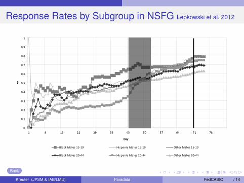
Response Rates by Subgroup in NSFG Lepkowski et al. 2012

Response Rates by Subgroup

0

0.1

0.2

0.3

0.4

0.5

0.6

0.7

0.8

0.9

1

1 8 15 22 29 36 43 50 57 64 71 78

Day

RR

Black Males 15‐19 Hispanic Males 15‐19 Other Males 15‐19

Black Males 20‐44 Hispanic Males 20‐44 Other Males 20‐44

Back


Automatically Generated Data

Structurally, an audit trail is a comma delimited text file, where each line in the audit trail (except for header information) shows the date and time when a keystroke was entered. An example of an audit trail for a case appears in Figure 1. Figure 1: Excerpt from an audit trail file "1/11/2004 9:15:50 AM","Enter Form:1","Key:XXXXXXXX " "1/11/2004 9:15:50 AM","Metafile name:C:\WINCM\DATA\STUDIES\CEQ_BA01\e-inst\inst.bmi" "1/11/2004 9:15:50 AM","Metafile timestamp:Wednesday, December 03, 2003 8:47:42 AM" "1/11/2004 9:15:50 AM","WinUserName:FR" "1/11/2004 9:15:50 AM","Enter Field:Front.Start","Status:Normal","Value:" "1/11/2004 9:16:13 AM","Leave Field:Front.Start","Cause:Next Field","Status:Normal","Value:5" …….. "2/11/2004 5:52:21 PM","Enter Field:Sect03.ANYRENT","Status:Normal","Value:" "2/11/2004 5:52:24 PM","Leave Field:Sect03.ANYRENT","Cause:Next Field","Status:Normal","Value:2" …… "1/11/2004 6:16:42 PM","Enter Field:Back.Appt.verify_info","Status:Normal","Value:" "1/11/2004 6:16:43 PM","Leave Field:Back.Appt.verify_info","Cause:Next Field","Status:Normal","Value:1" "1/11/2004 6:16:44 AM","Leave Form:1","Key:XXXXXXXX " Keystrokes entered into the CAPI instrument are identified by keywords in the audit trails; examples of keywords appear in Figure 2. Figure 2: Example of Audit Trail Keywords KEYWORD DESCRIPTION KEYWORD DESCRIPTION

Key Case identifier Enter Field Identifies the name of the field (question) entered

Enter Form Enter case Leave Field Identifies the name of the field (question) left

Leave Form Leave case Value The value entered for the field Transforming the audit trails into a more structured format The text format of the audit trails necessitated sequential scanning of these files to access file contents. To perform complex analysis and to optimize queries, the audit trails were transformed into a more structured format for faster random access to information in the audit trails. Hierarchical database structure for SAS data sets We came up with a hierarchical data base structure to store the audit trails audit based by the following characteristics:

1. One audit trail represents one case (an interview with a respondent) 2. A case could take one or more sessions to complete. Within each case, the start of a session is delineated with the

audit trail keyword "ENTER FORM", and the end of a session by the keyword "LEAVE FORM" 3. Within each session, the interviewer enters questionnaire responses and administrative information as the survey is

administered. The relevant keywords that identify these keystrokes are "ENTER FIELD", "LEAVE FIELD", and "ACTION".

SAS was used to read and parse the audit trails into the following 5 tables (SAS data sets):

• CASE: Each record represents one case, and contains the line number and date-time stamp of start of first entry into the case and last exit from the case.

• FORM: Each record represents one session in a case; so there are as many records for a case as there were sessions to complete the case. Each record shows the line numbers and date-time stamps for the start and end of that session.

• ACTION: Each record represents ACTION keystrokes in a case. Each record shows the date-time stamp, line number, field on which the ACTION keystroke was triggered, the type of action, and resulting value of the action (if any).

Back


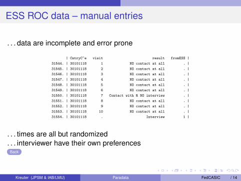
ESS ROC data – manual entries

. . . data are incomplete and error prone

Sequence analysis: ESS

Step 3: Check for sequence length

• Reshape and manually removing missing cases at the end

• Merge with substantive ESS file on CntryCase (IDvar) andresult (result=1 for ESS)

| CntryC~e visit result fromESS |

31544. | 30101118 1 NO contact at all . |

31545. | 30101118 2 NO contact at all . |

31546. | 30101118 3 NO contact at all . |

31547. | 30101118 4 NO contact at all . |

31548. | 30101118 5 NO contact at all . |

31549. | 30101118 6 NO contact at all . |

31550. | 30101118 7 Contact with R NO interview . |

31551. | 30101118 8 NO contact at all . |

31552. | 30101118 9 NO contact at all . |

31553. | 30101118 10 NO contact at all . |

31554. | 30101118 . Interview 1 |

by CntryCase (visit): replace visit = visit[ n-1] + 1 if mi(visit)

Essex 2007 10. . . times are all but randomized. . . interviewer have their own preferences

Back


World Health Survey 2002 – paper entry

0350. Contact record

Number of calls

A. Date (day / month / year)

B. Day of week

C. Exact time began

D. Interviewer I.D.

E. Contact with

F. Mode of contact

G. Tel. Number if obtained

H. Household Unit listing obtained

I. Detailed description of contact or attempt to contact

J. Result code

Number of calls

A. Date (day / month / year)

B. Day of week

C. Exact time began

D. Interviewer I.D.

E. Contact with

F. Mode of contact

G. Tel. Number if obtained

I. Detailed description of contact or attempt to contact

J. Result code

H. Househol Unit listing obtained

S0350 CALL #1

__ __ / __ __ / __ __ __ __

Respondent Informant No One

1 2 3

Personal Telephone

1 2

Yes No

1 5

S0351 CALL #2

__ __ / __ __ / __ __ __ __


1 2 3

Personal Telephone

1 2

Yes No

1 5

S0352 CALL #3

__ __ / __ __ / __ __ __ __


1 2 3

Personal Telephone

1 2

Yes No

1 5

S0353 CALL #4

__ __ / __ __ / __ __ __ __


1 2 3

Personal Telephone

1 2

Yes No

1 5

S0354 CALL #5

__ __ / __ __ / __ __ __ __


1 2 3

Personal Telephone

1 2

Yes No

1 5

S0359 CALL #10

__ __ / __ __ / __ __ __ __ __ __ / __ __ / __ __ __ __ __ __ / __ __ / __ __ __ __ __ __ / __ __ / __ __ __ __ __ __ / __ __ / __ __ __ __

S0355 CALL #6 S0356 CALL #7 S0357 CALL #8 S0358 CALL #9

Respondent Informant No One Respondent Informant No One Respondent Informant No One Respondent Informant No One Respondent Informant No One

1 2 3 1 2 3 1 2 3 1 2 3 1 2 3

Personal Telephone Personal Telephone Personal Telephone Personal Telephone Personal Telephone

1 2 1 2 1 2 1 1 2

Yes No Yes No Yes No Yes

1 5 1

2

51 5 1 5 1 5

No Yes No

WORLD HEALTH SURVEY - CONTACT RECORD - S C.5


CHI - Census Bureau

Back


NHIS CHI Doorstep Data Maitland et al. 2009

interviewers forget to record variables or some of them might be difficult to observe. The factor analysis approach might help smooth out this measurement error by using multiple variables to measure a latent tendency for someone to express a certain type of concern. Table 4 shows the resulting correlations of the factor scores with survey participation and the survey variables. As expected, the factors based on the individual paradata variables are more strongly correlated with survey participation than the survey variables. The general resistance factor is the strongest correlate with participation. The average correlation between the factor scores and the survey variables is approximately .03. The largest correlation is .15. Table 4. Correlation of factor scores with participation and survey variables (2006 data).

Correlation with survey variables (absolute values) Variable set Correlation with

participation Average Maximum

Cooperation Factor 1: Time concerns -.25 .03 .09 Factor 2: Privacy or content concerns -.27 .02 .09 Factor 3: General resistance -.47 .02 .12 Factor 4: Gatekeeper issues -.30 .02 .08 Contactability Factor 1: Contact problems or effort -.25 .03 .15 Factor 2: Location or barrier issues -.24 .02 .12

We also looked at the correlation of the individual paradata variables with participation. The top half of Table 5 shows that the cooperation variables are better correlates with participation than the contactability variables. The strongest correlates with participation are the indicators for the sample person indicating they are not interested or do not want to be bothered (-.69) and the sample person hangs up or slams the door on the interviewer (-.64). The bottom half of the table summarizes the correlations between the paradata variables and the vector of survey variables. The average correlations are only in the .02-.07 range. Only in a few cases are the correlations larger than .2. We also ran separate logistic regression models on the contactability and cooperation variables to obtain a response propensity for each case based on these variables. However, these propensities were not correlated any stronger with the survey variables than many of the individual paradata variables.

Back


Measurement Error: Gender McCulloch & Kreuter 2012

Pooled data: 28 CATI surveys (n=25,635), Marist College (MIPO):

Respondent Respondent Totalmale female

Guess - male 97.36 13.87 49.63Guess - female 2.64 86.13 50.37

Total 100.00 100.00 100.00

White Afr. Am. Hispanic Asian OtherGuessed Correct 92.1% 87.4% 92.1% 92.0% 92.7%Guessed Incorrect 7.9% 12.6% 7.9% 8.0% 7.3%


ρ Interviewer vs. ρ Census Tract Casas-Cordero et al. 2012

14

Fig. 3. Estimates of Intraclass Correlation from the Linear Unconditional Models

NG watch sign

Security signs

Tended yards

Graffiti

Cigarettes

Security gates

Litter, glass

Cond. bldgs.

Trash, junk

Aband. cars

Damaged walls

Drug items

Empty bottles

Dog sign

Painted graff

Vacant lots

Boarded up

Bars on windows

0 .2 .4 .6 .8 1

ρint ρsp

Intra Class Correlations


Measurement Error: Young Children West & Kreuter 2012

NSFG Interviewer Observations from 16 Quarters (n=15,044):

Back


paradata within the total survey error framework … (jpsm & iab/lmu) paradata fedcasic 2 / 14....

Documents