pareto governors for energy-optimal computing

6

Pareto Governors for Energy-Optimal Computing

RATHIJIT SEN and DAVID A. WOOD, University of Wisconsin-Madison

�e original de�nition of energy-proportional computing does not characterize the energy e�ciencyof recent recon�gurable computers, resulting in non-intuitive “super-proportional” behavior. �is paperintroduces a new de�nition of ideal energy-proportional computing, new metrics to quantify computationalenergy waste, and new SLA-aware OS governors that seek Pareto optimality to achieve power-e�cientperformance.

CCS Concepts: •General and reference →Metrics; Performance; •Hardware →Power and energy;Power estimation and optimization;

Additional Key Words and Phrases: DVFS, prefetching, SLA, RAPL, performance-per-wa�

ACM Reference format:Rathijit Sen and David A. Wood. 2017. Pareto Governors for Energy-Optimal Computing. ACM Transactionson Architecture and Code Optimization 14, 1, Article 6 (March 2017), 25 pages.DOI: 0000001.0000001

1 INTRODUCTION

We see that peak energy e�ciency occurs at peak utilization and drops quickly asutilization decreases.

Luiz Andre Barroso and Urs Holzle [3]

Energy e�ciency is the work done per unit amount of energy used. Maximizing energy e�ciencyallows more work to be done for a given energy budget and also allows work to be done faster fora given power budget. �is has economic and environmental bene�ts as it minimizes the energyneeded to do a given computation.

Barroso and Holzle [3] observed that real systems—at that time—a�ain peak e�ciency at peakutilization, but quickly lose e�ciency as utilization drops as they are unable to proportionatelyreduce power consumption. �ey posit that an “ideal” energy-proportional system should alwaysuse energy in proportion to the work done, by maintaining this peak e�ciency even at reducedload.

Figures 1a and 1b illustrate this original model for an Intel Haswell server running SPECpower [36].�e points labeled with Peak Performance Con�guration show the server’s power-performance atdi�erent load levels with the highest processor frequency. �e machine can serve maximum load(peak performance) with this con�guration. �e EP line represents Barroso and Holzle’s “ideal”

�is work was supported in part by the National Science Foundation, under grant CCF-1218323, grant CNS-1302260, andgrant CCF-1533885.Author’s addresses: R. Sen, Gray Systems Lab, Microso� Corporation; D. A. Wood, Department of Computer Sciences,University of Wisconsin-Madison.Permission to make digital or hard copies of all or part of this work for personal or classroom use is granted without feeprovided that copies are not made or distributed for pro�t or commercial advantage and that copies bear this notice andthe full citation on the �rst page. Copyrights for components of this work owned by others than ACM must be honored.Abstracting with credit is permi�ed. To copy otherwise, or republish, to post on servers or to redistribute to lists, requiresprior speci�c permission and/or a fee. Request permissions from [email protected].© 2017 ACM. XXXX-XXXX/2017/3-ART6 $15.00DOI: 0000001.0000001

ACM Transactions on Architecture and Code Optimization, Vol. 14, No. 1, Article 6. Publication date: March 2017.

6:2 R. Sen et al.

energy-proportional pro�le where performance is linearly proportional to power. We consider thisa design ideal for future systems, since current systems have unavoidable idle power consumption.�e Dynamic EP line accounts for idle power [26], and represents an operational ideal for thecurrent system. �is server’s Peak Performance Con�guration achieves power-performance veryclose to Dynamic EP. Figure 1b shows that the corresponding energy e�ciency (η), normalizedto that at peak performance, reduces quickly from 100% as performance drops. In contrast, an EPsystem is always 100% e�cient.

0

20

40

60

80

100

0% 20% 40% 60% 80% 100%

Syst

em

Po

we

r (W

)

Load (% Peak Performance)

Peak Perf.

Con g.

Dynamic EP

EP

(a)

0%

20%

40%

60%

80%

100%

120%

140%

0% 20% 40% 60% 80% 100%

En

erg

y E

cie

ncy

()

(No

rma

lize

d)


Peak Perf.

Con g.

EP

(b)

Fig. 1. (a) Power vs Load and (b) E�iciency vs Load for conventional systems.

0

20

40

60

80

100

0% 20% 40% 60% 80% 100%

Syst

em

Po

we

r (W

)


Peak Perf.

Con g.

Other

Con gs

Dynamic EP

EP

Pareto

Fron er

Super-Propor onal

Sub-Linear

max_L

max_P

(a)

0%

20%

40%

60%

80%

100%

120%

140%

0% 20% 40% 60% 80% 100%

En

erg

y E

cie

ncy

()

(No

rma

lize

d)


Peak Perf.

Con g.

Other

Con gs

EP

Pareto

Fron er

Super-Propor onalSuper-Propor onal

max_L

max

(b)

Fig. 2. (a) Power vs Load and (b) E�iciency vs Load for super-proportional systems.

Barroso and Holzle’s observation has been instrumental in helping drive recent system designsto have lower idle power and a wide dynamic power range. However, their model describes systemswith �xed resources, while these modern, more-e�cient processors have recon�gurable resources—e.g., core frequencies, voltages, number of active cores, threads per core, etc. that can be variedat runtime. Operating such a server with �xed resources can be ine�cient when it faces variableloads. Load variation can occur due to �uctuating demands, or service consolidation and loadbalancing among other servers [7, 9, 28].

Servers achieve maximum performance when con�gured for peak performance (Peak Perfor-mance Con�guration), but other con�gurations can trade performance for greater energy e�ciency.Figures 2a and 2b show that changing just the socket frequency (and consequently voltage) results inenergy e�ciency that exceeds the “ideal” EP pro�le. Speci�cally, by varying the frequency from 3.9to 0.8 GHz, the server can achieve super-proportional e�ciency over almost 60% of the performance


Pareto Governors for Energy-Optimal Computing 6:3

range (points in the shaded Super-Proportional region—where performance is super-proportionalto power). Figure 2b shows that the maximum e�ciency, ηmax, is 29% higher relative to the EPenergy e�ciency for this server. ηmax occurs at load ηmax L (which is approximately two-thirds ofmaximum load) and power consumption ηmax P.

Recon�gurable systems create opportunities for increased e�ciency even outside the super-proportional region. For example, Figure 2b shows that the Peak Performance Con�guration a�ainsa relative e�ciency of 61% at 30% load, while a di�erent con�guration achieves a relative e�ciencyof 88% at the same load. In other words, the usual server con�guration uses 44% more energy thannecessary to satisfy the same load, despite being nearly on the Dynamic EP line.

�us, neither EP nor Dynamic EP (that is, the conventional ideal models) describes the fullpotential of modern computing systems. While non-linearity with recon�guration is well-known,e.g., with frequency (and voltage) control, the existing ideal models do not consider its impact onpeak e�ciency. We propose new ideal models to address this limitation.

Conventional energy proportionality metrics are de�ned using conventional ideals and havelimitations for super-proportional systems. A popular metric, EP metric1 [32, 45], compares thearea between the power-performance curves of a real server relative to that of the “ideal” energy-proportional server to quantify how close the real server is to the “ideal” server. Depending onthe shapes of their power-performance curves, a super-proportional server can have a EP metricvalue close to that of a sub-proportional server. �us, EP metric does not identify all servers thatcan bene�t from scheduling policies that exploit super-proportionality (e.g., policies other thanrace-to-halt).

Recent works [30, 44] have proposed schedulers that can exploit super-proportionality, butcontinue to use the conventional ideals for energy proportionality. Di�ering goals and idealscan create confusion in scheduling applicability. For example, although Wong [44] observes thatthe peak e�ciency is higher than the “ideal” (conventional energy proportional) e�ciency, andoccurs at intermediate utilizations, they propose the Peak E�ciency Aware Scheduler (PEAS) “forhighly energy proportional servers” (identi�ed using EP metric). Our rede�ned notion of energyproportionality removes this semantic ambiguity. In our framework the ideal model achieves peake�ciency.EP metric does not quantify excess energy used by the real server compared to the least possible

at a given load level. Another metric, Proportionality Gap (PG) [45], is parametrized by theutilization level, x%, and is de�ned as:

PGx% =Poweractual@x% − Powerideal@x%

Powerpeak

For a conventional non-recon�gurable server, PGx% ≥ 0. However, for a recon�gurable super-proportional server, PG turns out to be negative for utilizations in the super-proportional region ifthe conventional ideal model is used. We �nd this mix of positive and negative values non-intuitivefor a metric to quantify room for improvement in energy proportionality of an actual server withrespect to an ideal model.

Another limitation of PG is that it does not quantify the load allocation and server con�gurationaspects of suboptimality in a�ained energy e�ciency. Separation of these aspects is useful sinceenergy e�ciency for a server in a cluster can be a�ected both by inter-server load distribution aswell as intra-server con�guration selection decisions. Our new metrics quantify these e�ects foreach server. Together they in�uence how much computational energy a server is using relative toits optimum.

1�e metric is called EP in the cited papers, but we use EP metr ic in this discussion to di�erentiate it from the EP model.


6:4 R. Sen et al.

�is paper describes an analytical framework that integrates the concepts of energy proportion-ality, energy optimality, Pareto e�ciency, peak e�ciency, ideals for system designers and operators,lower bounds on energy consumption, and develops new mechanisms that meet user-speci�edService-Level Agreements (SLAs) while minimizing computational energy.

�e main contributions of this work are:(1) New Ideals: We propose new ideals for both system designers and system operators.

Energy Optimal Proportional (EOP) is the new design ideal that subsumes conventional“ideal” energy proportionality. Dynamic Energy Optimal (Dynamic EO), that is the power-performance Pareto frontier, is the new operational ideal.

(2) New Metrics: We propose a new metric called Computational Power Usage E�ectiveness(CPUE) to quantify excess computational energy used with respect to that by EOP. We alsopropose new metrics, Load Usage E�ectiveness (LUE) and Resource Usage E�ectiveness(RUE), that can help system operators to focus on load management and con�gurationmanagement to make the system operate e�ciently. We develop the “Iron Law of Energy”that quanti�es the impact of poor load management (a�ecting LUE) and poor con�gurationmanagement (a�ecting RUE) on CPUE.CPUE mirrors the well-known datacenter-level PUE metric [1] for a server’s computa-tional energy consumption. Just as datacenter operators aim to reduce PUE, server op-erators/schedulers should try to reduce CPUE either by reducing LUE or RUE or both.Scheduling policies can reach target CPUE levels by governing for one or both of theseaspects a�er taking into account additional constraints such as data movement costs forstateful services.

(3) New Governors: We develop new OS governors that seeks Pareto-optimality for socketfrequency (and associated voltage) scaling and hardware cache prefetching. OS governorscurrently do not control hardware prefetching.

2 TERMINOLOGY, INFRASTRUCTURE, ANDWORKLOADSSimilar to Barroso and Holzle [3, 4], we de�ne energy e�ciency as Work

Energy , or equivalently, PerformancePower .

�e performance of a system is measured as the rate of doing work, e.g., the load served, transactionscompleted, or instructions executed per unit time. We refer to 100% load as the maximum loadachieved for the Peak Performance Con�guration (all cores at the highest frequency and prefetchingenabled). All loads are normalized with respect to that peak load. �e normalized load is the systemutilization [3].

�e system that we use is a single-socket quad-core Haswell Xeon E3-1275 v3 server with 32GB memory (DDR3-1600), henceforth referred to as HS. HS runs RHEL 2.6.32. It has a frequencyrange of 0.8–3.9 GHz with 3.5+–3.9 GHz being the turbo boost region. �e turbo boost plan is2/3/4/4 meaning that the maximum frequency can be 3.5 + 0.1*2 = 3.7 GHz with all four coresactive, 3.5 + 0.1*3 = 3.8 GHz with three cores active, and 3.5 + 0.1*4 = 3.9 GHz with two or onecores active. We run the system with all four cores, hyperthreading (thus, 8 threads per socket),and cache prefetching enabled by default. All cores run at the same frequency (HS does not supportper-core DVFS). �e socket frequency can changed in steps of 100 MHz by writing to Model Speci�cRegisters (MSRs). Any value for the turbo region limits the maximum frequency. HS has a socketTDP of 84W, socket idle power of 0.27W, and DRAM idle power of 4.3W.

�e OS acpi-cpufreq interface allows controlling frequency in 15 steps from 0.8–3.5 GHz (0.8–2.0GHz and 2.1 GHz–3.5 GHz in steps of 200 MHz) and enabling/disabling the turbo boost region(3.5+ GHz). We use this granularity while comparing with the existing Linux governors (Section 9onwards). We use the �ner granularity of 100 MHz elsewhere and also in Section 11.3.



0

20

40

60

80

100

0% 20% 40% 60% 80% 100%

Syst

em

Po

we

r (W

)


Dynamic EP

EP

Dynamic EO

EOP

Super-Propor onal

Sub-Linear

max_L

max_P

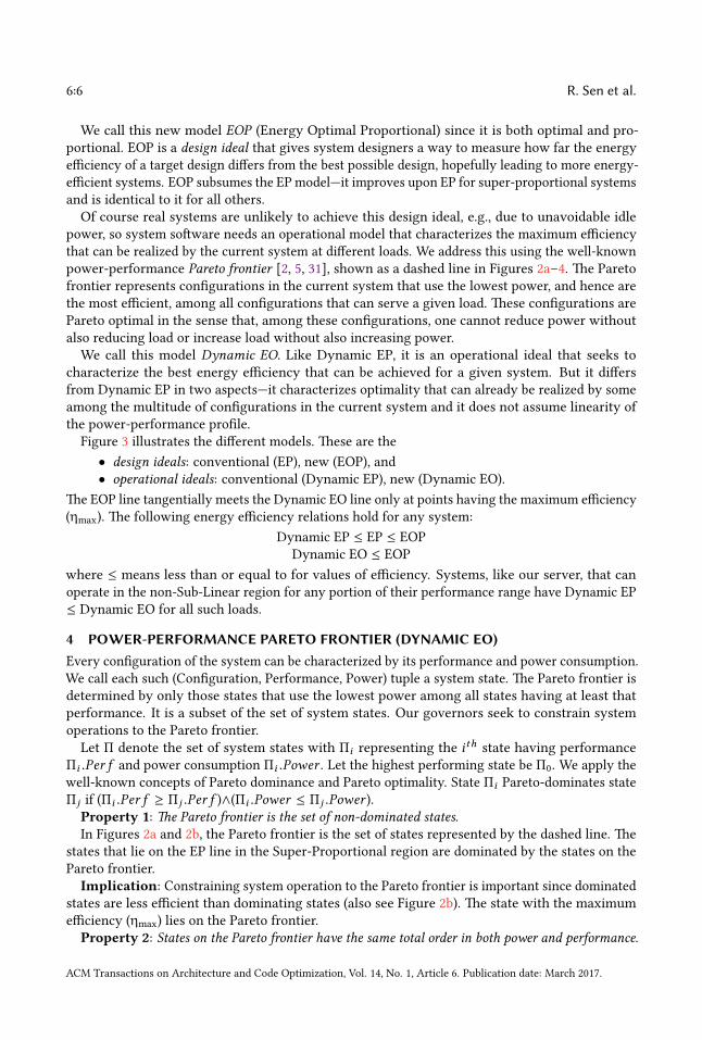
Fig. 3. EOP and Dynamic EO models.

We measure socket power and DRAM power using an additional so�ware thread that readsavailable RAPL (Runtime Average Power Limit) counters [19, 21] at 1 second intervals. �is runsas a thread separate from application threads and any governor threads. �e governors that wedevelop also read RAPL counters for power calculations. We measure wall power with a Wa�s Up?(.net) meter [12] at 1 second intervals. �is also runs as a separate additional thread for experimentswhere we use wall power.

We run the SPECpower benchmark [36]. �is Java workload simulates warehouse transactionprocessing, with (by default) as many warehouses as logical processors on the system under test,that is, the server. Transaction requests to each warehouse arrive in batches of 1000 transactionseach. �e batches have (negative) exponentially distributed interarrival times. �e server load ismeasured in total transactions per second. �e workload �rst calibrates the maximum, or 100%,load. Next, it does measurement intervals by varying the load o�ered to the system under testfrom 100% (max. utilization) to 0% (no utilization) in decrements of 10%. In these intervals, the loadserved must be within 2% (up to 2.5% shortfall for the 100% and 90% intervals is allowed) of theo�ered load. SPECpower uses its own so�ware daemon to periodically measure and report systempower in the measurement intervals.

We also run graph500 [14], hpcg [11, 33], and 14 workloads from SPECOMP2012 [37]. graph500and SPECpower are run fully whereas the other workloads are run for the �rst 1200 seconds (a fewruns of kdtree complete within this time at high frequencies).

3 REDEFINING EP AND DYNAMIC EP�e EP model assumes that maximum energy e�ciency occurs at maximum (100%) load andargues that an ideal system should achieve that e�ciency for all loads. Yet Figure 2b shows that arecon�gurable server actually a�ains maximum e�ciency (ηmax) at a lower load (ηmax L < 100%).We argue that a be�er ideal model is one that achieves this optimal e�ciency ηmax for all loads.

Similar to the EP model, the ideal system should have maximum e�ciency (ηmax) at every load.�is implies that for a given computation, it will use minimum energy (Emin) to do it irrespective ofthe computing rate (performance or load). Figure 3 shows its geometric interpretation as a straightline passing through the points (0, 0) and (ηmax L, ηmax P). �is ideal system, that is energy optimalat every load, uses power linearly proportional to load (l/ηmax power at load l ). Energy optimalityat every load implies energy proportionality, but the converse is not true, e.g., EP is proportionalbut not optimal at all loads.


6:6 R. Sen et al.

We call this new model EOP (Energy Optimal Proportional) since it is both optimal and pro-portional. EOP is a design ideal that gives system designers a way to measure how far the energye�ciency of a target design di�ers from the best possible design, hopefully leading to more energy-e�cient systems. EOP subsumes the EP model—it improves upon EP for super-proportional systemsand is identical to it for all others.

Of course real systems are unlikely to achieve this design ideal, e.g., due to unavoidable idlepower, so system so�ware needs an operational model that characterizes the maximum e�ciencythat can be realized by the current system at di�erent loads. We address this using the well-knownpower-performance Pareto frontier [2, 5, 31], shown as a dashed line in Figures 2a–4. �e Paretofrontier represents con�gurations in the current system that use the lowest power, and hence arethe most e�cient, among all con�gurations that can serve a given load. �ese con�gurations arePareto optimal in the sense that, among these con�gurations, one cannot reduce power withoutalso reducing load or increase load without also increasing power.

We call this model Dynamic EO. Like Dynamic EP, it is an operational ideal that seeks tocharacterize the best energy e�ciency that can be achieved for a given system. But it di�ersfrom Dynamic EP in two aspects—it characterizes optimality that can already be realized by someamong the multitude of con�gurations in the current system and it does not assume linearity ofthe power-performance pro�le.

Figure 3 illustrates the di�erent models. �ese are the• design ideals: conventional (EP), new (EOP), and• operational ideals: conventional (Dynamic EP), new (Dynamic EO).

�e EOP line tangentially meets the Dynamic EO line only at points having the maximum e�ciency(ηmax). �e following energy e�ciency relations hold for any system:

Dynamic EP ≤ EP ≤ EOPDynamic EO ≤ EOP

where ≤ means less than or equal to for values of e�ciency. Systems, like our server, that canoperate in the non-Sub-Linear region for any portion of their performance range have Dynamic EP≤ Dynamic EO for all such loads.

4 POWER-PERFORMANCE PARETO FRONTIER (DYNAMIC EO)Every con�guration of the system can be characterized by its performance and power consumption.We call each such (Con�guration, Performance, Power) tuple a system state. �e Pareto frontier isdetermined by only those states that use the lowest power among all states having at least thatperformance. It is a subset of the set of system states. Our governors seek to constrain systemoperations to the Pareto frontier.

Let Π denote the set of system states with Πi representing the ith state having performanceΠi .Per f and power consumption Πi .Power . Let the highest performing state be Π0. We apply thewell-known concepts of Pareto dominance and Pareto optimality. State Πi Pareto-dominates stateΠj if (Πi .Per f ≥ Πj .Per f )∧(Πi .Power ≤ Πj .Power ).Property 1: �e Pareto frontier is the set of non-dominated states.In Figures 2a and 2b, the Pareto frontier is the set of states represented by the dashed line. �e

states that lie on the EP line in the Super-Proportional region are dominated by the states on thePareto frontier.

Implication: Constraining system operation to the Pareto frontier is important since dominatedstates are less e�cient than dominating states (also see Figure 2b). �e state with the maximume�ciency (ηmax) lies on the Pareto frontier.Property 2: States on the Pareto frontier have the same total order in both power and performance.



Let Πi ,Πj be states on the Pareto frontier. �en (Πi .Per f > Πj .Per f ) ⇐⇒ (Πi .Power >Πj .Power ). We number the states in decreasing order of performance. �e ordering relation forstates on the frontier is thus: i < j ⇐⇒ (Πi .Per f > Πj .Per f ) ∧ (Πi .Power > Πj .Power ).

Implication: While the state space is two-dimensional, the Pareto frontier is more constrainedallowing system operators to qualitatively reason about the other dimension from looking at onedimension alone. For example, increasing the power budget will improve performance at the Paretofrontier if the power is used. �is is not true for the whole state space where states with lessperformance can use more power. �is positive correlation between the two dimensions exists atthe Pareto frontier.

Property 3: System states that optimize power-performance metrics are located at the Paretofrontier.

Consider a state Πi that is not on the frontier. So there exists at least one other state Πj such thatΠi .Per f ≥ Πj .Per f and Πi .Power ≤ Πj .Power with at least one of the inequalities being strict.�is implies that the highest performing state with/without a (maximum) power cap and the lowestpower state with/without a (minimum) performance bound lie on the Pareto frontier.

In this work we assume that per f ormance ∝ delay−1. Since energy is power multiplied by time(delay), it implies that the lowest energy point with/without a delay cap must lie on the Paretofrontier. Since the state corresponding to the highest performance-per-wa� is the same as the statewith the lowest energy, that state will also be on the Pareto frontier. Moreover, according to theabove condition, states corresponding to the minimum energy-delay (ED) product or ED2 productor, in fact, any EDn ,n ≥ 0 must also lie on the Pareto frontier.

Since Pareto-optimal states are more e�cient than other states, the highest performing statewith/without a maximum power cap, the lowest power state with/without a minimum performancebound, the highest performance-per-wa� state, the lowest energy state, the lowest energy-delaystate, etc. will lie on the Pareto frontier.

Implication: Optimizing system operations for commonly used power-performance or energye�ciency metric necessitates operating it at the Pareto frontier.

Property 4: �e points of contact between the frontier, Power = f (Per f ), and the tangent curvePower = cn (Per f )

n+1,n + 1 ≥ 0 and some constant cn , represent con�gurations that optimize(minimize) metric EDn . (n = 0 means energy E.)

Let Πi be a state that optimizes (minimizes) metric EDn . By Property 3, Πi must be on thefrontier. Since E = Power (Per f )−1 and EDn = Power (Per f )−n−1, Πi will be on the curve for thepower function Power = cn (Per f )

n+1 if we choose cn = Πi .Power (Πi .Per f )−n−1. cn is thus the

optimum value for EDn . Moreover, every point on this power function curve will have the samevalue for EDn , which is cn . No part of the frontier can be below this curve, as then states on thispart of the frontier will have lower power for the same performance compared to points on thepower function curve directly above them and thus have a smaller value for EDn than cn which isa contradiction.

All points on the curve above the linear tangent are suboptimal with respect to E, all pointsabove the quadratic tangent are suboptimal with respect to ED, all points above the cubic tangentare suboptimal with respect to ED2, and so on.

Implication: �is forms the basis for the geometric interpretation of the EOP line described inSection 3. Every point on the linear tangent has the same slope, which is equal to Power

Performance , thatis, performance-per-wa�−1 value of the most energy-e�cient point.Property 5: �e Pareto frontier is not necessarily convex (or concave).


6:8 R. Sen et al.

Let Πi ,Πj ,Πk be states on the frontier with i < j < k . �e ordering relations only implyΠi .Per f > Πj .Per f > Πk .Per f and Πi .Power > Πj .Power > Πk .Power , not Πj .Power ≤

Πk .Power +(Πj .Per f −Πk .Per fΠi .Per f −Πk .Per f

)(Πi .Power − Πk .Power ).

Implication: Convex optimization approaches cannot be directly applied while composing mul-tiple Pareto frontiers. Moreover, hill-climbing based search techniques at the frontier can get stuckin local optima instead of reaching global optima. However convex (polynomial) approximationsto the Pareto frontier may work well.

5 COMPUTATIONAL PUEDatacenters can satisfy a given load by distributing it to machines in di�erent ways. Each machinecan also be con�gured in a large number of ways. �ese modes for servicing the load di�er in theamount of energy consumed, since some modes are more ine�cient than others. A hypotheticalideal system, that is, one that meets the design ideal EOP, achieves maximal energy e�ciency (ηmax)and thus minimizes the energy (Emin) needed for a given computation regardless of load. We wouldlike a metric to quantify the excess energy used by a real system, compared to this ideal system.

Our new metric, Computational Power Usage E�ectiveness (or, CPUE), measures how much energya server uses with con�guration c at load l compared to the energy used by EOP. We de�ne

CPUE(c,l ) = Actual server energy with c at lEOP energy at l , l > 0 (1)

=E(c,l )Emin

, l > 0 (2)

�us,E(c,l ) = CPUE(c,l ) × Emin, l > 0 (3)

CPUE(c,l ) is inspired by the well-known PUE metric [1] that tracks energy waste for datacentersby taking the ratio of facility energy consumption to energy consumption by IT equipment. PUE >1 quanti�es excess relative energy used by the datacenter due to the non-IT infrastructure. Similarly,CPUE(c,l ) > 1 quanti�es excess relative computational energy used whenever e�ciency dropsbelow ηmax.

We de�ned CPUE(c,l ) as E(c,l )/Emin. We will now decompose CPUE(c,l ) to focus on two majorfactors that cause ine�ciencies: i) running the system at a non-optimal load and ii) for a givenload, running the system with a non-optimal con�guration. For a given amount of work, energyconsumed is inversely proportional to e�ciency. �us,

CPUE(c,l ) = ηmaxη(c,l )

, l > 0 (4)

=

(ηmax

ηPareto (l )

)×

(ηPareto (l )

η(c,l )

), l > 0 (5)

= LUE(l ) × RUE(c,l ), l > 0 (6)�us,E(c,l ) = LUE(l ) × RUE(c,l ) × Emin, l > 0 (7)

where LUE(l ) denotes Load Usage E�ectiveness at load l and RUE(c,l ) denotes Resource UsageE�ectiveness of con�guration c and load l .

LUE(l) is the e�ciency of EOP (ηmax) relative to that of of Dynamic EO at load l . LUE(l ) ≥ 1with LUE(l ) = 1 ⇐⇒ l can be served at maximum e�ciency (ηmax). Since energy consumed isinversely proportional to e�ciency, LUE(l ) > 1 quanti�es excess energy consumed, relative to Emin,due to non-optimal loads assuming that the Pareto-optimal con�guration is used to serve load l .



RUE(c,l ) is the e�ciency of Dynamic EO relative to that of con�guration c , both at load l .RUE(c,l ) ≥ 1 with RUE(c,l ) = 1 ⇐⇒ c is a Pareto-optimal con�guration. RUE(c,l ) > 1 quanti�esexcess energy used, relative to Dynamic EO at load l , due to using non-optimal (Pareto-dominated)con�guration c for serving load l .

Our proposed RUE and LUE metrics can help system operators isolate the sources of energyine�ciency and guide new policies to reduce it. LUE is important for load management of Pareto-optimal con�gurations. RUE is important for con�guration management for Pareto-dominatedcon�gurations. While LUE is applicable to all systems, both old and new, it only partially quanti�esenergy waste in recon�gurable systems that can be con�gured in a plurality of ways. RUE completesthe quanti�cation. Both LUE(l ) and RUE(c,l ) can be expressed in terms of CPUE(c,l ). SinceRUEPareto (l ) = 1 for every l , LUE(l ) = CPUEPareto (l ) and RUE(c,l ) = CPUE(c,l )/CPUEPareto (l ).

Inspired by the “Iron Law of Performance”, we call Equation 7 the “Iron Law of Energy” tohelp with holistic management of server energy consumption. System designers will focus onminimizing Emin whereas system operators will focus on minimizing LUE and RUE.

6 LOAD AND CONFIGURATION MANAGEMENTMost data centers are provisioned to meet peak load, but normally operate at much lower load levels.�e LUE metric can help operators quantify the potential bene�t of deploying load managementpolicies [7, 9, 28, 44], e.g., concentrating load on some servers and shu�ing down others. Of course,any such policy must also ensure that service-level agreements are still satis�ed [30].

1

1.2

1.4

1.6

1.8

2

2.2

2.4

2.6

2.8

0% 20% 40% 60% 80% 100%

CP

UE

=

ma

x/


Peak Perf.

Con g.

Other

Con gs

Pareto

Fron er

(Dynamic

EO)

10% Loss at

Pareto Fron er

Fig. 4. CPUE(c,l ) and LUE(l ). These→ ∞ as load l → 0 due to non-zero idle power. For any configuration cand load l , CPUE(c,l ) ≥ CPUEPareto (l ) = LUE(l ) ≥ 1.

Figure 4 shows that CPUE for the Peak Performance Con�guration is always > 1 (wastes energy)and increases as load decreases. �e best CPUE for this con�guration is 1.29, occurs at peak load,and implies 29% excess energy used relative to Emin. LUE (that is, CPUE for Dynamic EO), on theother hand, �rst decreases to 1, then increases, revealing a sweet spot of ≤ 10% excess energy usedat around 51%–90% of peak performance.

Barroso and Holzle [3] observed that servers typically operate at 10%–50% load. �e LUE curvefor SPECpower (Figure 4), shows excess energy used due to suboptimal load of approximately10% at the higher end of this range, to over 250% (not shown) at the lower end. �e steep slopeof the LUE curve at low loads makes even modest load management very a�ractive. For example,


6:10 R. Sen et al.

1

1.1

1.2

1.3

1.4

1.5

1.6

0% 20% 40% 60% 80% 100%

RU

E =

CP

UE

/ C

PU

EP

are

to


Peak Perf.

Con g.

Other

Con gs

10% Loss

Fig. 5. RUE(c,l ).

increasing load from 10% to 20% of peak reduces LUE from 3.55 (255% excess) to 1.99 (99% excess)and a further increase to 25% peak load reduces LUE to 1.68 (68% excess).

Even in a data center with perfect load balancing, recon�gurable servers may be miscon�gured,wasting signi�cant energy even at optimal load. Figure 5 shows RUE for SPECpower for all systemcon�gurations and loads. Operating with the Peak Performance Con�guration is signi�cantlywasteful even at low loads, e.g., 21% excess energy used at 10% load compared to operating atDynamic EO. �e excess increases to 51% before decreasing to zero at peak load. Not all Pareto-dominated con�gurations are as wasteful—the shaded band identi�es con�gurations that have anRUE of ≤ 1.1 and hence limit the extra energy used to 10%.

7 PARETO GOVERNORSWe now develop new operating system governors (resource managers) that seek to operate thesystem at or close to Dynamic EO (power-performance Pareto frontier) so that Service-LevelAgreements (SLAs) are satis�ed. We call such governors Pareto governors. We consider the followingSLAs in this work.

• SLAee: Maximize energy e�ciency.• SLApower: Maximize performance given a power cap/budget.• SLAperf: Maximize power savings given a performance target.

Figure 6 shows what transitions the Pareto governors must make to the current operating pointto meet the SLAs. �e shaded regions in Figure 6a depict subsets of the system state space thatsatisfy a given power cap (for SLApower) or performance bound (for SLAperf). Figure 6b showsa special case for SLApower and SLAperf. �e special case of maximizing power savings for thesame performance a�ects only RUE but not LUE.

Our new governors, that meet these SLAs, have the following two-level design:(1) Pareto Predictor: �is predicts the power-performance Pareto frontier for the system and

currently observed execution pro�le.(2) Objective Selector: �is level selects the desired operating state from the Pareto frontier

according to the SLA to be achieved.�e objective selector remains unchanged if the available knobs change and the Pareto predictorremains unchanged if new SLAs are targeted. �is separation, due to Property 3 (Section 4) of thePareto frontier, simpli�es design and enhances portability.



SLAperf

Current configuration

SLAee

Performance

Po

we

r

Dynamic EO

EOP

SLApower

(a) General case

Maximize power savings for the same performance

Current configuration

Maximize energy efficiency

Performance

Po

we

r

Dynamic EO

EOP

Maximize performance for the same power

(b) Special case for SLApower and SLAperf.

Fig. 6. State transitions to Dynamic EO for meeting SLAs.

Our governors use the BIPS (Billion Instructions Per Second) throughput metric to determinecurrent application or to set performance targets. We assume the existence of user-suppliedso�ware routines that convert between BIPS and high-level performance metrics. Similar toexisting governors in Linux, our new governors do not keep track of higher-level applicationconstructs such transactions, queries, etc. �e workloads that we consider for our experimentsdo not have any latency constraints. Other workloads that have latency constraints on high-levelconstructs should estimate their BIPS requirement and communicate that to the governors.

8 EXISTING GOVERNORS IN LINUX�e Linux acpi-cpufreq module includes the following governors [6] that control the operatingfrequency. �e goal is to manage power-performance by either se�ing the frequency statically, orby varying it in response to processor utilization. With root privileges, the user can (dynamically)change the governor.

• PowerSave (S): Sets all cores to the lowest frequency. �e idea is to use the least amountof power to do the work, but performance may be less than what could be achieved on thismachine.

• OnDemand (O): Periodically samples (default: 10 ms interval) cores to adjust frequenciesbased on core utilization. �e idea is to reduce power by lowering frequency when the CPUis not fully utilized and increase frequency as utilization increases so that the performanceimpact is minimal. �e Conservative (C) governor is a variant of the OnDemand governorwith more conservative utilization thresholds for changing frequencies.• UserSpace (U): �e idea is to give the user (having root privileges) control of the frequency

se�ings. On HS, only the socket frequency (all cores together) can be set.• Performance (P): Sets all cores to the highest frequency. �e idea is to get the maximum

performance. �is governor also uses the maximum power.

To further distinguish between modes, we constrain U mode to exclude S or P mode frequencies,i.e., it operates in the range of 1.0–3.5 GHz. While these governors a�empt to control knobs(e.g., processor frequency) in the system, none of them seek to meet SLAs that deal with energyconsumption, power limits, or performance targets.


6:12 R. Sen et al.

9 SLAEE: MAXIMIZE ENERGY EFFICIENCYTemporarily, we consider system power as the sum of socket power and DRAM power, both ofwhich are estimated using RAPL counters.

HS exhibits signi�cant opportunities in improving BIPS/Wa� (equivalently, Instructions/nanoJoule)by changing frequency se�ings alone. BIPS changes between 1.18x (swim) to 4.86x (bwaves) ingoing from S to P modes whereas power changes between 2.52x (swim) to 5.67x (botsalgn), leadingto a BIPS/Wa� range of 1.29x (imagick) to 2.14x (swim) between best and worst values for thatworkload over all frequencies. For all these workloads, the minimum BIPS/Wa� happens for Pmode. applu and graph500 show a BIPS/Wa� range of 1.84x and 1.67x respectively (also see Figure7). We study SPECpower for SLAperf, but not for SLAee, as it must meet performance constraints.

To exploit the improvement potential, we propose a simple reactive, R(t), mode of operation.Our approach is to sample power and performance at a few di�erent frequencies, then use thatinformation to interpolate the frontier. �e Pareto frontiers are usually non-linear. �us, at leastthree samples are needed to target super-proportionality. In contrast, aiming for proportionalitywould require only two points, but the non-linearity in system behavior between the points couldnot be predicted or controlled.

We implement two power-performance predictors (in so�ware)—one for the socket subsystemand the other for the memory subsystem. �e socket predictor sets the frequency to 0.8 GHz (lowestfrequency), 2.1 GHz (midpoint frequency) and 3.5 GHz (nominal frequency) in three consecutiveintervals of t ms each and observes the power, performance, memory read and write bandwidthsfor each se�ing. It then interpolates the e�ects for the other frequencies.

A so�ware coordination module, running on one of the cores, reads the socket predictionsand DRAM predictions every 51t ms (immediately a�er the 3t socket sampling), composes thepredictions, estimates the frontier and selects the best frequency. �e length of the interval thatthe system runs in this state is 48t. It is during this time that the DRAM predictor is periodicallyinvoked (every 12t ms) to adjust a computed linear regression between DRAM power and readand write bandwidths (two variables) based on current readings. �e regression is reset every17 observations (204t ms) to react faster to phase changes. We choose this value since 17 is notdivisible by 4 (48t/12t = 4), so the regression will not be reset at the time when the readings areneeded for the power estimations with the interpolated values.

Since the optimal frequency will be in of the high/mid/low ranges, the sampling overhead isapproximately 2t

51t ≈ 4%. �e workload continues to execute, although suboptimally, in those twointervals, so the overhead is usually < 4%. For the intervals mentioned above, we do not accountfor additional governor overheads due to system calls, interpolation, estimations, etc. So, the actualintervals are slightly longer. �e governor in Section 11.3 accounts for these overheads.

�ere are three issues in implementing the interpolant for the socket predictor—ge�ing successivesamples having non-decreasing performance and power with increasing frequency, ge�ing sampleswith acceptable measurement noise/ji�er, and dealing with non-convexity of the frontier. �e �rstissue arises when the workload shows local phase behavior. �e second issue arises with rapidsampling that makes the ji�er in the energy measurements seem to be higher than that in thetiming measurements leading to occasionally unrealistic power numbers. �e third issue ariseswhen the number of samples is not enough to estimate the shape of the frontier well.

To deal with the �rst two issues, we disregard samples if either decreasing values are found or ifpower readings di�er in more than 10x between the three samples and the coordinator transitionsto 3.5 GHz. While other default actions are possible, we choose to penalize ourselves when weare not con�dent about the interpolation. On average (geometric mean) less than 2% of samples



are discarded, but the frequency can occasionally be high, e.g., 10% for bwaves in R(1). We do notcorrect for the third issue and our results will be suboptimal for non-convex frontiers.

1.36 1.36 1.39 1.53 1.37 1.47 1.42 1.42 2.14 1.29 1.87 1.84 1.60 1.41 1.67 1.95 1.55

0

0.1

0.2

0.3

0.4

0.5

0.6

0.7

0.8

0.9

1

md bwaves nab bt botsalgn botsspar ilbdc fma3d swim imagick mgrid applu smithwa kdtree graph500 hpcg geomean

S

O

U

P

(a) The Top line shows Performance-per-Wa� of the best U mode frequency relative to P mode

1.31 1.33 1.35 1.47 1.33 1.43 1.38 1.38 1.96 1.25 1.79 1.76 1.54 1.38 1.61 1.78 1.49

0

0.1

0.2

0.3

0.4

0.5

0.6

0.7

0.8

0.9

1


P

R(1)

R(4)

R(10)

R(20)

(b) The Top line shows Performance-per-Wa� of R(10) relative to P mode

Fig. 7. BIPS-per-Wa� on HS with di�erent policies.

Figure 7 compares the energy e�ciency (performance-per-wa�) with di�erent modes of operation.For all these workloads, the P mode has the lowest e�ciency. �e numbers at the top showmaximum gains (e.g., 1.36 implies 36% gains) in energy e�ciency over P-mode by selecting theoptimal frequency in U or S modes (Figure 7a) and R(10) mode (Figure 7b). We observe that:

• �e potential rewards for selecting optimal con�gurations are signi�cant: �e e�ciencyimprovements were 28.6% (imagick) to 113.7% (swim) over P (geometric mean: 55% overP, 13.4% over S). �e O and P modes are suboptimal for this metric for every workload.However, there is a performance cost. Compared to P mode, the most energy-e�cientfrequency se�ing for each workload resulted in a reduction of BIPS of around 12.8% (mgrid)to 45.3% (botsspar), with a geometric mean of 35.4%.

• �ere is no single best static frequency se�ing: �e best static frequency se�ings for thedi�erent workloads were 0.8 GHz (swim), 1.0 GHz (applu, graph500, hpcg), 1.4 GHz (mgrid),1.8 GHz (bt, botsspar), 2.0 GHz (ilbdc, smithwa, kdtree), 2.1 GHz (md, nab, botsalgn, fma3d),2.3 GHz (bwaves, imagick).

• Rapid pro�ling and recon�gurations are not necessary for long running workloads: We dida sensitivity analysis with t = 1 ms, 4 ms, 10 ms, and 20 ms. �e resulting performance-per-wa� numbers indicate that R(20) (geometric mean: 48% over P, 8.3% over S), R(10)(geometric mean: 49% over P, 9% over S), and R(4) (geometric mean: 48.7% over P, 8.8%over S) improved over R(1) (geometric mean: 27.5% over P, -6.7% over S).


6:14 R. Sen et al.

We found that many workloads exhibit long-term variation and periodic behavior in power-performance traces. For example, applu shows 34.3 sec periodicity in P mode and 42.3 sec withR(10). graph500 exhibits 12.3 sec periodicity in P-mode and 15 sec with R(10). We expect longtraining intervals that track considerable execution history to work well with such workloads.

We use quadratic interpolation for the socket predictor. A piecewise linear interpolation wouldbe faster, but for the performance-per-wa� metric, only one of the sample frequencies (0.8/2.1/3.5GHz) would get chosen as the optimal frequency. �is is because Per f ( f ) = af + b, Pwr ( f ) =c f + d =⇒ Per f ( f )/Pwr ( f ) is monotonic in f. So, the maxima will always occur among the endpoints of the interval. For applu, while Linear �uctuates mostly between 0.8 and 2.1 GHz, resultingin 66% improvement over P-mode, �adratic selects more frequencies in between resulting in76.4% improvement. mgrid similarly had more improvements with �adratic than with Linear.

Doing �xed-time experiments (running for 1200 secs), as opposed to �xed-work experiments,risks ge�ing incomparable runs. However, for these workloads, the di�erences are small due tostability in the average energy e�ciency over long time intervals. We re-evaluated results usingthe same number of instructions (minimum across all policies from the �xed-time runs) for eachworkload. In terms of U-mode gains over P-mode, applu changed from 84% to 80% whereas botssparchanged from 47% to 52%. �e geometric mean changed < 2% for all policies. All trends remainedthe same.

9.1 SLAee: Adding L2 Prefetch ControlHardware prefetching on Intel x86 machines can be enabled or disabled by writing speci�c values toModel-Speci�c Registers (MSRs) [20]. All prefetchers are enabled by default. In this study we keepthe DCU (L1 Data Cache) prefetchers enabled, but dynamically enable or disable the L2 prefetchers(all cores).

0

10

20

30

40

50

60

70

80

0 5 10 15 20 25

So

cke

t +

Me

m P

ow

er

(W)

Performance (BIPS)

MD

DVFS+L2 Prefetch

DVFS+No L2 Prefetch

0

10

20

30

40

50

60

70

80

0 5 10 15 20

So

cke

t +

Me

m P

ow

er

(W)

Performance (BIPS)

MGRID

DVFS+L2 Prefetch

DVFS+No L2 Prefetch

Fig. 8. Pareto-optimal states have L2 prefetching enabled for mgrid, but not for md.

Figure 8 shows one example workload each for bene�cial prefetch (mgrid) and harmful prefetch(md) with all possible socket DVFS se�ings. When prefetching is disabled, md shows 14% improve-ment in peak performance and 13.6% in maximum energy e�ciency whereas mgrid shows 12.3%loss in peak performance and 14.9% loss in maximum energy e�ciency. Disabling prefetch alsoimproves SPECpower performance (Figure 14). Since prefetching bene�ts are workload dependent,a static prefetch se�ing will always be suboptimal for some workloads.

We extend the frequency governor in the following simple way. Instead of taking one sampleat 2.1 GHz, we take two samples—once with prefetching enabled and once disabled. We choosethe prefetching mode that gives be�er performance and continue with that for the remaining twosamples and estimating the frontier for that interval. Our choice of 2.1 GHz for taking the initialtwo samples is motivated by the need to keep the overhead of taking an extra sample small. A



mid-range frequency, such as 2.1 GHz, is likely to incur a lower additional overhead for this thana high frequency, such as 3.5 GHz since the energy-e�cient operations for most workloads arenot at high frequencies. Similar to R(t), we name the new governor RF(t) (Reactive with prefetchcontrol), parametrized by t, the length of the pro�ling interval in milliseconds. RF(10) improvedperformance-per-wa� more than R(10) for md (48% over P instead of 31%) but did not createsigni�cant di�erences for other workloads.

To summarize, we �nd that the P, PF and O modes can always be improved by the otherpolicies. S works best for swim, well for hpcg, but can be improved by U, R and RF for the otherworkloads. U is a good policy to use provided that workload is known in advance and pro�lingexperiments can be carried out. R reaches close to U but is unable to outperform it. �is is likelybecause these workloads have long-term stable behavior making the best static frequency not a badchoice. On the other hand, R su�ers from runtime pro�ling overheads and prediction errors due tosampling inconsistency and non-convexity of the frontier. �e situation changes for SPECpower(see Sections 11.2 and 11.3), where reactive governors do signi�cantly be�er than static frequencyse�ings. RF further improves upon R if disabling prefetch is useful but does not hurt energye�ciency if not, so it represents the best of both prefetch modes.

9.2 SLAee: Adding Control for Wall PowerMeasuring wall power (to include power consumption by the PSU, network interfaces, hard disks,etc.) with external power meters causes a time granularity mismatch, e.g., minimum 1 sec intervalswith Wa�s Up? meters as opposed to milliseconds (supported by the RAPL counters) used by ourgovernors (R(10) uses a measurement interval granularity of 10 ms). So we estimate wall powerfrom socket+mem power (measured by RAPL counters) using regression models determined o�ineby running workloads (SPECOMP2012, graph500, hpcg) with all frequency se�ings. We considerthe following two models for wall power (y) as a function of socket+mem power (x ).

(1) �adratic: y = ax2 + bx + c . �e best-�t line is y = 0.004x2 + 0.7932x + 21.329 withcoe�cient of determination R2 = 0.9912.

(2) Linear: y = ax + b. �e best-�t line is y = 1.141x + 14.891 with R2 = 0.9869.�e quadratic model gives a be�er �t for idle power as well as a slightly be�er �t overall, so we usethis model for subsequent experiments.

1.24 1.18 1.15 1.34 1.16 1.22 1.17 1.19 1.67 1.09 1.57 1.56 1.44 1.20 1.33 1.50 1.30

0

0.1

0.2

0.3

0.4

0.5

0.6

0.7

0.8

0.9

1


P

RF(10)

Fig. 9. BIPS-per-wa� of governors P and RF(10) with wall (full-system) power.

Figure 9 shows the performance-per-wa� for the baseline P governor (measured wall power)and our new RF governor. RF reads RAPL counters, then applies the wall power model mentionedabove to estimate wall power. �e maximum gains in performance-per-wa� achieved by RFover P is 67% (swim) while the geometric mean over all workloads is 30.2%. Since CPUE is


6:16 R. Sen et al.

directly proportional to energy consumption and inversely proportional to energy e�ciency,we have CPU E (P)

CPU E (RF) =E (P)E (RF) =

η (RF)η (P) = 1.302. So the average energy savings of RF over P is

E (P)−E (RF)E (P) = 1 − E (RF )

E (P) = 1 − 1.302−1 = 23.2%. RF can thus save cost by using 23% less energy onaverage to do the same work or generate revenue by doing 30% more work on average for the sameenergy cost. While it improves energy-e�ciency, RF loses performance, with respect to P mode,ranging from 0.2% (md) to 30% (bt) with a geometric mean of 19.5%.

10 SLAPOWER: MAXIMIZE PERFORMANCEWITHIN A POWER CAP/BUDGETNone of the standard Linux governors S, C, O, U, P deal with power caps/limits. �e RAPL [21]capabilities include mechanisms to enforce a limit on the power consumption. One advantage ofRAPL limits over frequency se�ings is that they can be �ne-grained (e.g., units of 1/8 W) leading togreater control of the state space. Another advantage is that since RAPL limits are enforced by thehardware, the management overhead is lower than that of a so�ware-controlled governor. Priorworks [26, 39] have used power limiting as a mechanism to improve energy e�ciency.

�ere are two main disadvantages of the RAPL power-capping mechanisms. First, capping ofwall power cannot be directly speci�ed. Second, non-frequency se�ings (e.g., prefetching) arenot managed by the RAPL mechanisms. So, workloads such as md that bene�t signi�cantly fromprefetch control would not see those advantages with the RAPL approach. From this perspective,RAPL guarantees a power cap, not best performance within that power cap. Pareto optimalityprovides the stronger guarantee.

Our new governor for SLApower, RF SLApower(t), improves upon the RAPL governor inboth of these aspects. It controls both the prefetch se�ings as well as socket frequency to getthe maximum performance within a speci�ed power budget. We modify the objective selector toselect the next state that is predicted to use the highest power among all states with less powerconsumption than the SLA target. We do not set turbo mode frequencies because of limited controlin turbo mode, so our maximum frequency is the nominal frequency (3.5 GHz).

0

20

40

60

80

100

0 1 2 3 4 5 6

Fu

ll S

yst

em

Po

we

r (W

)

Performance (BIPS)

GRAPH500Socket DVFS

RF_SLApower

RAPL

Sub-Propor onal

Super-Propor onal

0

20

40

60

80

100

120

0 5 10 15 20

Fu

ll S

yst

em

Po

we

r (W

)

Performance (BIPS)

MDSocket DVFS+No L2 Prefetch

RF_SLApower

RAPL

Sub-Propor onal

Super-Propor onal

Fig. 10. Power-performance profiles for graph500 and md for SLApower.

We investigate enforcement of SLApower using RF SLApower(10) and the RAPL governorfor two of our workloads: graph500 and md. For RAPL, we limit average socket power over 1second intervals from 10W to 80W in steps of 5W. We could enforce a power cap only for thesocket on HS, not for the memory or for other components. We used caps on full system power forRF SLApower(10) (35W–80W for graph500 and 35W–105W for md, both in steps of 5W) and amore restrictive interval of 510 ms.

Figure 10 shows the power-performance pro�les for the governors. Both workloads exhibitedbehavior close to Pareto optimal with RF SLApower(10). �e RAPL governor works well for



graph500, but causes Pareto-dominated (hence suboptimal) operations for md as it does not controlprefetch se�ings. RF SLApower(10) falls short of achieving maximum performance at the upperend of the operating range due to not operating in the turbo region.

11 SLAPERF: MAXIMIZE POWER SAVINGS GIVEN A PERFORMANCE TARGETNone of the standard governors S, C, O, U, P deal with user-speci�ed performance targets. Our newgovernor, RF SLAperf(t), allows the user to specify performance targets in absolute or relative(with respect to peak) BIPS.

11.1 Governing for absolute performance targetsTo govern for this SLA, we keep the Pareto predictor intact, but modify the objective selectorto keep track of the performance so far (time elapsed and instructions executed). �e idea is todetermine the desired performance for the next interval so that if this target is met, then the averageperformance so far would be that required by the SLA. If the average performance so far is greaterthan the SLA, the lowest performing point is chosen. Otherwise, if the next interval target is greaterthan the best performance predicted for 3.5 GHz, then turbo mode is chosen. Otherwise, the pointon the frontier that meets or just exceeds the next interval target is chosen.

We investigate enforcement of SLAperf using RF SLAperf(10) for two of our workloads: mdand graph500. md has mostly homogeneous behavior during its execution and we will show that itcan be governed well to meet the SLA. On the other hand, graph500 has signi�cant heterogeneity(di�erent execution phases) and, as we shall show, cannot be governed well without prior knowledgeof the phase behavior.

md has an average performance range of 4.8–21.6 BIPS at the frontier depending on the frequencyand with L2 prefetching disabled. We select SLA targets of 5.0, 7.5, 10.0, 12.5, 15.0, 17.5, 20.0 and22.5 BIPS (unreachable). graph500 has an average performance range of 2.9–5.6 BIPS at the frontierdepending on the frequency and with L2 prefetching enabled. We select SLA targets of 3.0, 3.5, 4.0,4.5, 5.0 and 5.5 BIPS.

0

20

40

60

80

100

120

0 5 10 15 20

Fu

ll S

yst

em

Po

we

r (W

)

Performance (BIPS)

MDSocket DVFS+No L2 Prefetch

RF_SLAperf

Sub-Propor onal

Super-Propor onal

0

10

20

30

40

50

60

70

80

0 1 2 3 4 5 6

Fu

ll S

yst

em

Po

we

r (W

)

Performance (BIPS)

GRAPH500Socket DVFS

RF_SLAperf

Sub-Propor onal

Super-Propor onal

Fig. 11. Power-performance profiles for md and graph500 for SLAperf.

Figure 11 shows the power-performance pro�les and expected behavior for both workloads. �epro�le for md was at the frontier except at high performance targets. Its highest performance isaround 3.5% less than the maximum possible due to sampling/pro�ling and prediction overheadsin the governor. For targets close to its highest performance, it tries to compensate for the lossby transitioning more into turbo mode resulting in more power consumption and consequently,Pareto-dominated states.

�e governor failed to meet the SLA for most points of graph500 and the pro�le was quitesuboptimal, being closer to proportional than Pareto optimal. However, as we explain below,


6:18 R. Sen et al.

this is primarily due to the non-homogeneous nature of the workload rather than incorrect statetransitions chosen by the governor.

0

10

20

30

40

50

60

70

0

2

4

6

8

10

12

14

16

18

20

0 200 400 600 800 1000 1200 1400

Wa

BIP

S

Seconds

BIPS Avg. BIPS SLA BIPS Socket+Mem Power

0

10

20

30

40

50

60

70

0

2

4

6

8

10

12

14

16

18

20

0 200 400 600 800 1000

Wa

BIP

S

Seconds

BIPS Avg. BIPS SLA BIPS Socket+Mem Power

Fig. 12. Execution traces for graph500 with SLA = 3.5 BIPS and 5.5 BIPS.

Figure 12 shows execution traces for graph500 for two SLAs: 3.5 and 5.5 BIPS. �e primaryvertical axis (le� axis) and the blue line show the number of instructions executed per second inBIPS. �e secondary vertical axis (right axis) and the red line show the power (socket+memory) inWa�s. �e Avg. BIPS line shows the average BIPS a�ained by the workload execution so far. �edashed line shows the average BIPS expected to be reached over the entire execution. �e governorseeks state transitions that will maintain the average BIPS equal to the SLA BIPS.graph500 has non-homogeneous behavior—the initial approximately 290 seconds is mostly a

high-performance phase whereas the remainder of the execution (successive iterations of breadth-�rst search) is low-performance. Initially, the average BIPS is higher than the SLA BIPS, so thegovernor reduces frequency to the lowest possible to save power. Eventually, execution enters thelow-performance phase and the average BIPS starts dropping more rapidly. However, the governorcontinues with a low frequency execution as the SLA BIPS is still lower than the average BIPS.A�er a while (1152 seconds for SLA=3.5, 491 seconds for SLA=5.5), the average drops below theSLA BIPS and remains that way although the governor transitions to higher frequencies includingturbo mode (with a sharp increase in power consumption). �is is more pronounced for SLA=5.5,where the SLA is breached earlier, than for SLA=3.5. Timely prediction of maximum performancein future execution phases is needed to handle this issue.

11.2 Governing for relative performance targetsFigure 13 shows power-performance pro�les for SPECpower with the default governors. P-modeand O-mode perform similarly and use the highest power for the achieved load. S-mode uses thelowest power for the achieved load, but the maximum load achievable is low (see below). C-modeworks be�er than P-mode or O-mode at low loads but in general consumes signi�cantly morepower than S-mode or the U-mode Pareto frontier for the same load. For these experiments we“niced” the power measurement daemon and set the ignore nice load parameter of the O and Cgovernors to discount activity by the daemon while calculating processor utilization.

Even though S-mode’s pro�le lies on the Pareto frontier, it has two limitations. First, it can onlyserve up to around 27% of peak load. So it will fail the performance requirement (see Section 2)at higher loads. �e other governors in Figure 13 can serve high as well as low loads. Second,although RUE = 1 for this governor, LUE ≥ 1.58. So, at least 58% excess energy is used comparedto operating with the best load even though it is operating at the Pareto frontier. Its pro�le doesnot even enter the Super-Proportional region. So, restricting servers to this policy is not a good



0

20

40

60

80

100

120

0 50 100 150 200 250 300 350 400

Fu

ll S

yst

em

Po

we

r (W

)

ssj_ops (Thousands)

SPECpowerP modeO modeC modeS modeU mode Pareto Fron er

Sub-Propor onal

Super-Propor onal

Fig. 13. Power-performance profiles for SPECpower with Linux governors.

idea. �e other governor pro�les are distant from Dynamic EO, thus have large RUE values (wasteenergy).

To govern for this SLA, we modify the Pareto predictor to also sample turbo mode so that peakBIPS can be estimated. We now have the maximum pro�ling frequency as 3.7 GHz (midpoint ofthe turbo range 3.5–3.9 GHz) since we do not know the actual temperature-dependent operatingfrequency. For any load, the target relative BIPS is set to be equal to that load level (load relative tomaximum load). For example, a�empting to serve 70% load level sets the target relative BIPS to 0.7.�e objective selector selects the lowest-power con�guration that is predicted to have relative BIPSgreater than or equal to the target relative BIPS.

We call this new governor RF SLAperf(t). �e parameter t, in milliseconds, is the length of theintervals as follows. For 100% target performance, the plan is to turn prefetching o� and on for t mseach, then choose the mode that performed be�er to run with for the next 48t ms. �is plan is thenrepeated. For 100% target performance, the frequency is kept at 3.7 GHz and not changed. For alower target performance, the plan is to set frequency to 2.1 GHz (midpoint frequency) for pro�lingprefetch se�ings (t ms for each mode). With the chosen prefetching mode, set frequency to 3.7GHz (turbo frequency) and then to 0.8 GHz (lowest frequency) for t ms each. We then estimate thePareto frontier, select the best frequency, and run with that se�ing for the next 48t ms.

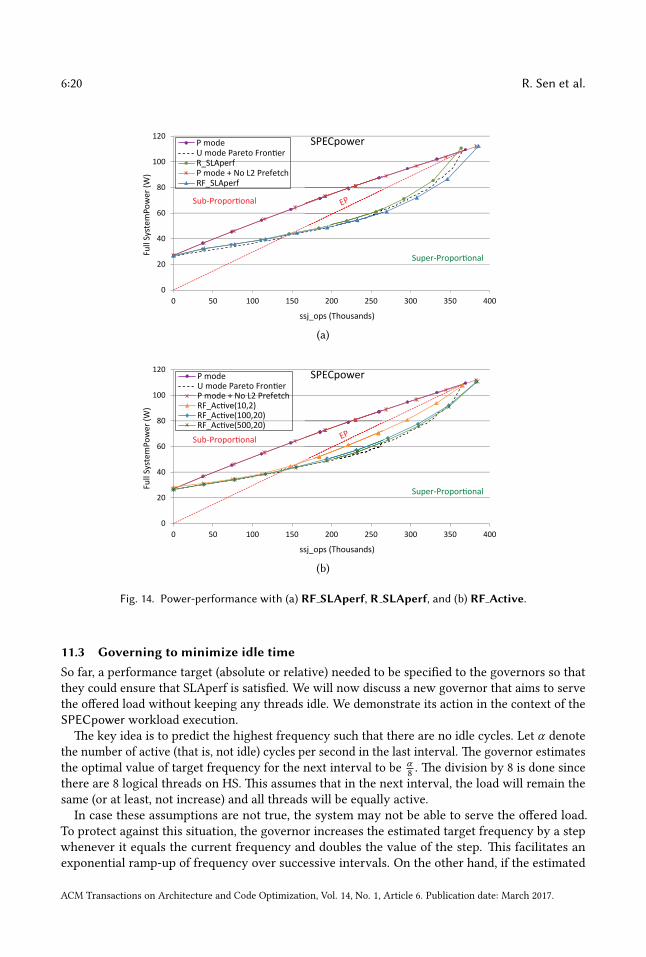
Figure 14a shows power-performance withR SLAperf(10) andRF SLAperf(10). R SLAperf(t)always enables prefetching whereas RF SLAperf(t) dynamically controls it. Controlling prefetch-ing increases the maximum load achievable compared to P-mode that always has prefetchingenabled. RF SLAperf(10) outperforms P-mode by around 4%. �is outcome is qualitatively similarto md (See Figure 10). �e increase in maximum performance can also be observed by running inP-mode with prefetching disabled (P-mode + No L2 Prefetch pro�le).

RF SLAperf(10) disabled prefetching for most of the time and chose a number of di�erentfrequencies for each run depending on the load served. By default, SPECpower does 3 calibrationintervals followed by 11 measurement intervals. During the calibration intervals and the �rstmeasurement interval, the server is o�ered very high load. So we expect that during these timesthe maximum frequency would be chosen by the governor. �us for at least (3+1)/(3+11) = 28.6%(observed: 34%) of the time, the maximum frequency should be chosen. �e last measurementinterval is “Active Idle”, that is zero load is o�ered, so we expect to select the lowest frequencyduring this interval which is around 1/(3+11) = 7.1% (observed: 15%) of total time.


6:20 R. Sen et al.

0

20

40

60

80

100

120

0 50 100 150 200 250 300 350 400

Fu

ll S

yst

em

Po

we

r (W

)

ssj_ops (Thousands)

SPECpowerP mode

U mode Pareto Fron er

R_SLAperf

P mode + No L2 Prefetch

RF_SLAperf

Sub-Propor onal

Super-Propor onal

(a)

0

20

40

60

80

100

120

0 50 100 150 200 250 300 350 400

Fu

ll S

yst

em

Po

we

r (W

)

ssj_ops (Thousands)

SPECpowerP modeU mode Pareto Fron erP mode + No L2 PrefetchRF_Ac e(10,2)RF_Ac e(100,20)RF_Ac e(500,20)

Sub-Propor onal

Super-Propor onal

(b)

Fig. 14. Power-performance with (a) RF SLAperf, R SLAperf, and (b) RF Active.

11.3 Governing to minimize idle timeSo far, a performance target (absolute or relative) needed to be speci�ed to the governors so thatthey could ensure that SLAperf is satis�ed. We will now discuss a new governor that aims to servethe o�ered load without keeping any threads idle. We demonstrate its action in the context of theSPECpower workload execution.

�e key idea is to predict the highest frequency such that there are no idle cycles. Let α denotethe number of active (that is, not idle) cycles per second in the last interval. �e governor estimatesthe optimal value of target frequency for the next interval to be α

8 . �e division by 8 is done sincethere are 8 logical threads on HS. �is assumes that in the next interval, the load will remain thesame (or at least, not increase) and all threads will be equally active.

In case these assumptions are not true, the system may not be able to serve the o�ered load.To protect against this situation, the governor increases the estimated target frequency by a stepwhenever it equals the current frequency and doubles the value of the step. �is facilitates anexponential ramp-up of frequency over successive intervals. On the other hand, if the estimated



target frequency is less than the current frequency, the frequency is set to the target frequency andthe step is re-initialized.

We call our new governor RF Active(t,p). It repeatedly does the following. It turns prefetchingo� and on for p/2 ms each. �en it chooses the prefetching mode that performed be�er and alsoestimates and sets the frequency for the remaining interval. We determine the length of the lastinterval o�ine so that the average total epoch length is t ms including governor overheads (systemcalls, pro�ling, and estimations). �is governor does not predict either power or performance forany con�guration, but manages to operate the system very close to Dynamic EO.

Figure 14b shows the power-performance pro�le of our new governor, RF Active, with di�er-ent parameter values: RF Active(10,2), RF Active(100,20), and RF Active(500,20). For theseexperiments, we consider all frequencies (0.1 GHz granularity). RF Active(10,2) su�ers from moreoverheads and less accurate selection of resource se�ings with shorter intervals—it keeps prefetch-ing enabled for a larger fraction of time and also selects the maximum frequency more o�en thanRF Active(100,20) or RF Active(500,20). Compared to RF SLAperf(10), RF Active(100,20)and RF Active(500,20) select the lowest frequency more o�en and the maximum frequency lesso�en but keep prefetching enabled for longer.

RF Active is similar to PAMPA [42] since both governors change core frequency in response tocore utilization. �e description of PAMPA does not include the rate of frequency change in eachstep, but we believe that our exponential ramp-up strategy allows RF Active to increase servicerates faster in response to a sudden increase in load levels. PAMPA controls the number of activecores in addition to core (socket) frequency but does not control cache prefetch enable. Number ofactive cores as well as thread placement [41] are interesting resource management knobs that canenhance the potentials for power savings.

12 LIMITATIONSWe will now discuss a few limitations of our governor designs—socket-wide control, intrusivepro�ling, sampling inconsistency, non-zero reaction times, and not tracking latency distributions.

Socket-Wide Control: Our governors select the same resource se�ing for the entire socket.Having the same frequency se�ing for all cores may be suboptimal for non-homogeneous workloadsif the hardware supports di�erent se�ings for di�erent cores. We expect that we can continueto pro�le with all-core se�ings and then predict per-core Pareto frontiers. To do that we need tomeasure or estimate, using performance counter values, the performance and energy consumptionof each core for each pro�led se�ing. But interpolating Pareto frontiers individually for many corescan be costly in so�ware. Hardware support for doing this would be useful.

Intrusive Pro�ling: Our governors try out a few resource con�gurations (e.g., socket fre-quencies) to determine their e�ectiveness. �is intrusive pro�ling may be costly in terms ofrecon�guration latency and energy for some resources, e.g., caches. Moreover, exhaustively pro-�ling a multitude of resources can be prohibitively expensive for short time intervals. To limitoverheads, pro�ling can be combined with other strategies, such as analytical models and heuristics,to guide resource con�guration decisions. For example, thread criticality can be used to partitionaggregate frequency among cores [27]. CoScale [10] uses analytical performance and energy modelsparametrized by pro�led values of performance counters and activity counters at the highest coreand memory frequencies.

Sampling Inconsistency: �e strategy of sampling execution with three frequencies and then��ing a quadratic polynomial to the measured power-performance values assumes that the samplesare consistent, that is, not drawn from di�erent execution phases. Sample inconsistency can beavoided by an alternate approach [34, 38] that samples performance counters once, then predicts


6:22 R. Sen et al.

power and performance for other con�gurations using a precharacterized model. However, thatapproach is limited by the number of performance counters that can be concurrently read (cana�ect prediction accuracy) and by the availability of the particular counters on di�erent platforms(can a�ect portability).

Non-Zero Reaction Times: Our R(t) governors logically partition execution time into epochs,of length 51t or 52t. Shortening the epochs will allow for faster reaction times with increasedpro�ling overhead. However, they need to be long enough to capture a stable, representative regionof workload execution. Moreover, the unit of time, t, cannot be made very small due to limitedupdate frequency of the RAPL counters (usually about once every millisecond [15, 21]).

Latency Distribution Unawareness: Our governors track performance in terms of throughputmetrics but not in terms of distributions of computation latency/response times. However, some on-line applications such as web services may have requirements on tail latency that need to be met [8].Recent works [17, 23, 24, 26, 29, 30] have explored latency-aware resource management (withoutprefetching control). We plan to augment our governors to be aware of latency requirements,possibly with application-speci�c knowledge, as part of future work.

13 RELATEDWORKHsu and Poole [16] observed real machines doing be�er than the conventional “ideal” system thatassumes linear proportionality. �ey proposed quadratic proportionality (Power(u) ∝ u2, where u isthe load level) as the new ideal model. However, this makes ideal system e�ciency load-dependent(

uPower(u ) =

1u

), with higher e�ciency at lower loads than at higher loads. Wong also observed that

the peak e�ciency can occur at intermediate loads, in the super-proportional region [44].Wong and Annavaram [45] name the region that we call Sub-Linear as Superlinear. We prefer to

use “Sub-” in the sense that operating in this region lowers e�ciency compared to that of Linear(Dynamic EP).

Song et al. [35] proposed Iso-energy-e�ciency (EE) as the energy ratio between sequentialand parallel executions of a given application. Our CPUE, LUE and RUE metrics do not usespeci�c execution modes (e.g., sequential/parallel, homogeneous/heterogeneous, speculative/non-speculative, cache-conscious/cache-oblivious, etc.) for reference, but compare system states tothe Pareto frontier (Dynamic EO) or to EOP. �e de�nitions of our metrics are oblivious to whichcon�gurations created the frontier. �e EE model focuses on maintaining equal e�ciency assystems and applications scale up. In contrast, the EP and EOP models focus on maintaining equale�ciency under changing loads. EE does not quantify its dependence on load.

Barroso and Holzle [4] compute datacenter energy consumption as PUE × SPUE × energy toelectronic components. While PUE accounts for non-compute overheads in datacenter buildinginfrastructure, SPUE (Server PUE) accounts for overheads, e.g., power supply losses, to computingenergy. Our RUE and LUE metrics do not separate SPUE losses from computing energy but separateenergy-wasting operating con�gurations and loads from optimal ones.

Other existing metrics [32, 40, 45] for characterizing energy e�ciency, e.g., based on the dynamicpower range, ratio between the idle and peak power consumptions, deviations from or area enclosedby an ideal curve, etc. continue to be useful with the new ideals, EOP and Dynamic EO, replacingthe conventional ideals.

Dynamic voltage and frequency scaling (DVFS) and dynamic frequency scaling (DFS) for coresare well-known techniques [13, 18, 43]. Researchers have explored mechanisms [10, 22, 24, 27, 30]to exploit per-core DVFS capabilities. Our server, HS, lacks this support (also see Section 12).

OS governors [6, 34, 38] typically control DVFS se�ings but not additionally prefetch se�ings.



Seeking Pareto optimality for improving e�ciency is well-known [2, 5, 25, 31, 44], but itsrelationship to energy proportionality had not been formalized (see Section 3 for invariants betweenDynamic EP, EP, Dynamic EO and EOP).

14 CONCLUSIONPower-performance Pareto optimality and energy proportionality are well-known but dissimi-lar concepts, both of which share the end goal of making computing more energy e�cient. Wedemonstrated that the conventional model of energy proportionality is inadequate for recon�g-urable systems since it does not guarantee energy optimality. We de�ned a new model, EOP, thatguarantees both optimality and proportionality and established its relation to the Pareto frontier.

We proposed a new metric, Computational PUE (CPUE), that quanti�es how much excesscomputational energy is used by real systems relative to that by EOP. �is depends on both the loadserved and the system con�guration used to serve that load. Our new Iron Law of Energy showshow CPUE can be decomposed into constituent terms that help separate the load, con�guration,and design aspects of suboptimality.

We developed new SLA-aware OS governors that seek Pareto optimality, and thereby reduceCPUE, in the presence of frequency scaling and cache prefetching. We demonstrated improvementsin performance-per-wa� by up to 67% (maximum gains) and 30% on average (geometric mean overall workloads) of a modern Intel Haswell server machine. �is opens up signi�cant opportunitiesfor revenue generation or cost savings. We also presented case studies and discussed challenges ingoverning for maximizing performance within a power cap and minimizing power for a performancetarget. Scheduling frameworks that carefully choose con�gurations and operating ranges willunlock the full potential of current and future recon�gurable systems.

ACKNOWLEDGMENTSWe thank Luiz Barroso, Edouard Bugnion, Mark Hill, Michael Marty, Kathryn McKinley, MichaelSwi�, and anonymous reviewers for helpful comments. �is work was supported in part bythe National Science Foundation, under grant CCF-1218323, grant CNS-1302260, and grant CCF-1533885. �e views expressed herein are not necessarily those of the NSF. Wood has signi�cant�nancial interests in AMD and Google.

REFERENCES[1] Victor Avelar, Dan Azevedo, and Alan French (Eds.). 2012. PUE: A Comprehensive Examination of the Metric. �e

Green Grid.[2] Peter E. Bailey, Aniruddha Marathe, David K. Lowenthal, Barry Rountree, and Martin Schulz. 2015. Finding the Limits

of Power-constrained Application Performance. In Proceedings of the International Conference for High PerformanceComputing, Networking, Storage and Analysis (SC ’15). ACM, New York, NY, USA, Article 79, 12 pages.

[3] Luiz Andre Barroso and Urs Holzle. 2007. �e Case for Energy-Proportional Computing. Computer 40, 12 (Dec. 2007),33–37.

[4] Luiz Andre Barroso and Urs Holzle. 2009. �eDatacenter As a Computer: An Introduction to the Design ofWarehouse-ScaleMachines (�rst ed.). Morgan & Claypool Publishers.

[5] Luca Benini, Alessandro Bogliolo, Giuseppe A. Paleologo, and Giovanni De Micheli. 1999. Policy optimization fordynamic power management. IEEE Transactions on Computer-Aided Design of Integrated Circuits and Systems 18, 6(Jun 1999), 813–833.

[6] Dominik Brodowski and Nico Golde. 2015. CPU frequency and voltage scaling code in the Linux(TM) kernel. LinuxCPUFreq. CPUFreq Governors. h�ps://www.kernel.org/doc/Documentation/cpu-freq/governors.txt. (2015).

[7] Je�rey S. Chase, Darrell C. Anderson, Prachi N. �akar, Amin M. Vahdat, and Ronald P. Doyle. 2001. Managing Energyand Server Resources in Hosting Centers. In Proceedings of the Eighteenth ACM Symposium on Operating SystemsPrinciples (SOSP ’01). ACM, New York, NY, USA, 103–116.

[8] Je�rey Dean and Luiz Andre Barroso. 2013. �e Tail at Scale. Commun. ACM 56, 2 (Feb. 2013), 74–80.


https://www.kernel.org/doc/Documentation/cpu-freq/governors.txt

6:24 R. Sen et al.

[9] Christina Delimitrou and Christos Kozyrakis. 2014. �asar: Resource-e�cient and QoS-aware Cluster Management.In Proceedings of the 19th International Conference on Architectural Support for Programming Languages and OperatingSystems (ASPLOS ’14). ACM, New York, NY, USA, 127–144.

[10] Qingyuan Deng, David Meisner, Abhishek Bha�acharjee, �omas F. Wenisch, and Ricardo Bianchini. 2012. CoScale:Coordinating CPU and Memory System DVFS in Server Systems. In Proceedings of the 2012 45th Annual IEEE/ACMInternational Symposium on Microarchitecture (MICRO-45). IEEE Computer Society, Washington, DC, USA, 143–154.

[11] Jack Dongarra and Michael A. Heroux. 2013. Toward a New Metric for Ranking High Performance Computing Systems.Technical Report SAND2013-4744. Sandia National Laboratories.

[12] Electronic Educational Devices Inc. 20xx. Wa�s Up? .Net. h�ps://www.wa�supmeters.com/secure/products.php?pn=0&wai=0&spec=2. (20xx).

[13] Kinshuk Govil, Edwin Chan, and Hal Wasserman. 1995. Comparing Algorithm for Dynamic Speed-se�ing of aLow-power CPU. In Proceedings of the 1st Annual International Conference on Mobile Computing and Networking(MobiCom ’95). ACM, New York, NY, USA, 13–25.

[14] Graph 500. 2011. Graph 500 Reference Implementation v2.1.4. h�p://www.graph500.org/referencecode. (2011).[15] Marcus Hahnel, Bjorn Dobel, Marcus Volp, and Hermann Hartig. 2012. Measuring Energy Consumption for Short

Code Paths Using RAPL. SIGMETRICS Performance Evaluation Review 40, 3 (Jan. 2012), 13–17.[16] Chung-Hsing Hsu and S.W. Poole. 2013. Revisiting Server Energy Proportionality. In 2013 42nd International Conference

on Parallel Processing (ICPP). 834–840.[17] C. H. Hsu, Y. Zhang, M. A. Laurenzano, D. Meisner, T. Wenisch, J. Mars, L. Tang, and R. G. Dreslinski. 2015. Adrenaline:

Pinpointing and reining in tail queries with quick voltage boosting. In 2015 IEEE 21st International Symposium on HighPerformance Computer Architecture (HPCA). 271–282.

[18] Intel Corporation. 2004. Enhanced Intel SpeedStep Technology for the Intel Pentium M Processor. (March 2004).[19] Intel Corporation. 2012. Intel Performance Counter Monitor - A be�er way to measure CPU utilization. h�ps:

//so�ware.intel.com/en-us/articles/intel-performance-counter-monitor. (2012).[20] Intel Corporation. 2014. Disclosure of H/W prefetcher control on some Intel processors. h�ps://so�ware.intel.com/

en-us/articles/disclosure-of-hw-prefetcher-control-on-some-intel-processors. (September 2014).[21] Intel Corporation. 2015. Intel 64 and IA-32 Architectures So�ware Developer’s Manual, Vol. 3B: System Programming

Guide, Part 2. (2015).[22] Canturk Isci, Alper Buyuktosunoglu, Chen-Yong Cher, Pradip Bose, and Margaret Martonosi. 2006. An Analysis of

E�cient Multi-Core Global Power Management Policies: Maximizing Performance for a Given Power Budget. InProceedings of the 39th Annual IEEE/ACM International Symposium on Microarchitecture (MICRO 39). IEEE ComputerSociety, Washington, DC, USA, 347–358.

[23] Svilen Kanev, Kim Hazelwood, Gu-Yeon Wei, and David Brooks. 2014. Tradeo�s between Power Management andTail Latency in Warehouse-Scale Applications. In 2014 IEEE International Symposium on Workload Characterization(IISWC). 31–40.

[24] Harshad Kasture, Davide B. Bartolini, Nathan Beckmann, and Daniel Sanchez. 2015. Rubik: Fast Analytical PowerManagement for Latency-critical Systems. In Proceedings of the 48th International Symposium on Microarchitecture(MICRO-48). ACM, New York, NY, USA, 598–610.

[25] J. Li and J.F. Martinez. 2006. Dynamic power-performance adaptation of parallel computation on chip multiprocessors.In �e Twel�h International Symposium on High-Performance Computer Architecture. 77–87.

[26] David Lo, Liqun Cheng, Rama Govindaraju, Luiz Andre Barroso, and Christos Kozyrakis. 2014. Towards EnergyProportionality for Large-scale Latency-critical Workloads. In Proceeding of the 41st Annual International Symposiumon Computer Architecuture (ISCA ’14). IEEE Press, Piscataway, NJ, USA, 301–312.

[27] Kai Ma, Xue Li, Ming Chen, and Xiaorui Wang. 2011. Scalable Power Control for Many-core Architectures RunningMulti-threaded Applications. In Proceedings of the 38th Annual International Symposium on Computer Architecture(ISCA ’11). ACM, New York, NY, USA, 449–460.

[28] Jason Mars, Lingjia Tang, Robert Hundt, Kevin Skadron, and Mary Lou So�a. 2011. Bubble-Up: Increasing Utilizationin Modern Warehouse Scale Computers via Sensible Co-locations. In Proceedings of the 44th Annual IEEE/ACMInternational Symposium on Microarchitecture (MICRO-44). ACM, New York, NY, USA, 248–259.

[29] David Meisner, Christopher M. Sadler, Luiz Andre Barroso, Wolf-Dietrich Weber, and �omas F. Wenisch. 2011. PowerManagement of Online Data-intensive Services. In Proceedings of the 38th Annual International Symposium on ComputerArchitecture (ISCA ’11). ACM, New York, NY, USA, 319–330.

[30] George Prekas, Mia Primorac, Adam Belay, Christos Kozyrakis, and Edouard Bugnion. 2015. Energy Proportionalityand Workload Consolidation for Latency-critical Applications. In Proceedings of the Sixth ACM Symposium on CloudComputing (SoCC ’15). ACM, New York, NY, USA, 342–355.

[31] Martino Ruggiero, Andrea Acquaviva, Davide Bertozzi, and Luca Benini. 2005. Application-Speci�c Power-AwareWorkload Allocation for Voltage Scalable MPSoC Platforms. International Conference on Computer Design (ICCD)


https://www.wattsupmeters.com/secure/products.php?pn=0&wai=0&spec=2

https://www.wattsupmeters.com/secure/products.php?pn=0&wai=0&spec=2

http://www.graph500.org/referencecode

https://software.intel.com/en-us/articles/intel-performance-counter-monitor

https://software.intel.com/en-us/articles/intel-performance-counter-monitor

https://software.intel.com/en-us/articles/disclosure-of-hw-prefetcher-control-on-some-intel-processors

https://software.intel.com/en-us/articles/disclosure-of-hw-prefetcher-control-on-some-intel-processors


(2005), 87–93.[32] Frederick Ryckbosch, Stijn Pol�iet, and Lieven Eeckhout. 2011. Trends in Server Energy Proportionality. Computer 44,

9 (Sept. 2011), 69–72.[33] Sandia National Laboratories. 2014. High Performance Conjugate Gradients v2.1. h�ps://so�ware.sandia.gov/hpcg/

download.php. (Jan. 2014).[34] David C. Snowdon, Etienne Le Sueur, Stefan M. Pe�ers, and Gernot Heiser. 2009. Koala: A Platform for OS-level Power

Management. In Proceedings of the 4th ACM European Conference on Computer Systems (EuroSys ’09). ACM, New York,NY, USA, 289–302.

[35] S. Song, C. Y. Su, R. Ge, A. Vishnu, and K. W. Cameron. 2011. Iso-Energy-E�ciency: An Approach to Power-ConstrainedParallel Computation. In IEEE International Parallel Distributed Processing Symposium (IPDPS). 128–139.

[36] SPEC. 2008. SPECpower ssj. h�ps://www.spec.org/power ssj2008/. (2008).[37] SPEC. 2012. SPEC OMP2012. h�p://www.spec.org/omp2012/. (2012).[38] V. Spiliopoulos, S. Kaxiras, and G. Keramidas. 2011. Green governors: A framework for Continuously Adaptive DVFS.

In International Green Computing Conference and Workshops (IGCC). 1–8.[39] Balaji Subramaniam and Wu-chun Feng. 2013. Towards Energy-proportional Computing for Enterprise-class Server

Workloads. In Proceedings of the 4th ACM/SPEC International Conference on Performance Engineering (ICPE ’13). ACM,New York, NY, USA, 15–26.

[40] Georgios Varsamopoulos and Sandeep K. S. Gupta. 2010. Energy Proportionality and the Future: Metrics and Directions.In 39th International Conference on Parallel Processing Workshops (ICPPW). 461–467.

[41] Augusto Vega, Alper Buyuktosunoglu, and Pradip Bose. 2013. SMT-centric Power-aware �read Placement in ChipMultiprocessors. In Proceedings of the 22Nd International Conference on Parallel Architectures and Compilation Techniques(PACT ’13). IEEE Press, Piscataway, NJ, USA, 167–176.

[42] Augusto Vega, Alper Buyuktosunoglu, Heather Hanson, Pradip Bose, and Srinivasan Ramani. 2013. Crank It Up or DialIt Down: Coordinated Multiprocessor Frequency and Folding Control. In Proceedings of the 46th Annual IEEE/ACMInternational Symposium on Microarchitecture (MICRO-46). ACM, New York, NY, USA, 210–221.

[43] Mark Weiser, Brent Welch, Alan Demers, and Sco� Shenker. 1994. Scheduling for Reduced CPU Energy. In Proceedingsof the 1st USENIX Conference on Operating Systems Design and Implementation (OSDI ’94). USENIX Association, Berkeley,CA, USA, Article 2.

[44] Daniel Wong. 2016. Peak E�ciency Aware Scheduling for Highly Energy Proportional Servers. In Proceedings of the43rd Annual International Symposium on Computer Architecture (ISCA ’16).

[45] Daniel Wong and Murali Annavaram. 2012. KnightShi�: Scaling the Energy Proportionality Wall �rough Server-Level Heterogeneity. In Proceedings of the 2012 45th Annual IEEE/ACM International Symposium on Microarchitecture(MICRO-45). IEEE Computer Society, Washington, DC, USA, 119–130.

Received August 2016; revised December 2016; accepted January 2017


https://software.sandia.gov/hpcg/download.php

https://software.sandia.gov/hpcg/download.php

https://www.spec.org/power_ssj2008/

http://www.spec.org/omp2012/

pareto governors for energy-optimal computing

Documents