part 1 continuous-time butterworth...

FilterPoles

0.7071− 0.7071i+

0.7071− 0.7071i−

0.7071 0.7071i+

0.7071 0.7071i−

=

These are then the poles of |H(s)|^2.

FilterPoles polyroots DenomCoeffs( ):=

DenomCoeffs2 N⋅1

i Ωc⋅

2 N⋅:=DenomCoeffs0 1:=DenomCoeffsk 0:=

k 0 2 N⋅..:=

To use the Mathcad polyroots function,ceate a vector that contains the coefficients of the polynomial beginning with the constantterm and proceeding with increasing powers of s, i.e., a0 + a1 s + a2 s^2.

Ts1

Ωc:=Ωc 1:=N 2:=

To find the roots, first define the filter order, N, and cutoff frequency Ωc in radians/second

Dbutter s Ωc,( ) 1s

i Ωc⋅

2 N⋅+:=

The poles of |H(s)|^2 are at the roorts of the denominator, Dbutter() below

H s( )( )2 1

1s

i Ωc⋅

2 N⋅+

:=

Ωc

The Butterworth filter is defined by

Part 1Continuous-time Butterworth filter

(copyright T. Weldon, 2006)ECGR 6114Computer Project: filter design Student Name:___________

Part 2Plotting the poles and zeroes of continuous-time filter in the s-plane

and the pole-zero plot

ImagPoles Im FilterPoles( ):= RealPoles Re FilterPoles( ):=

Lets plot a unit circle too

un 0 40..:=ImagCircun Ωc sin 2 π⋅

un

40⋅

⋅:= RealCircun Ωc cos 2 π⋅un

40⋅

⋅:=

2 1 0 1 22

1

0

1

2

ImagPoles

ImagCirc

RealPoles RealCirc,

Q1. Replot for a Chebyshev filter with N=5, ε=0.5, Ωc=1, Ts=2/Ωc.

Part 3Finding the stable poles in the s-plane

The stable poles are in the left half plane and gibve rise to H(s) from |H(s)|^2

StablePoles vv( ) n rows vv( )←

cc 0←

xxcc vvnc← Re vvnc( ) 0<if

cc cc 1+← Re vvnc( ) 0<if

nc 0 n 1−..∈for

xx

:=

StableFilterPoles StablePoles FilterPoles( ):=

StableFilterPoles0.7071− 0.7071i+

0.7071− 0.7071i−

=

Q2. Find the stable poles for a Chebyshev filter with N=5, ε=0.5, Ωc=1, Ts=2/Ωc.

and the pole-zero plot of the stable poles

ImagPoles Im StableFilterPoles( ):= RealPoles Re StableFilterPoles( ):=


un 0 40..:=ImagCircun Ωc sin 2 π⋅

un

40⋅

⋅:= RealCircun Ωc cos 2 π⋅un

40⋅

⋅:=

2 1 0 1 22

1

0

1

2S-plane plot of poles

ImagPoles

ImagCirc

RealPoles RealCirc,


Part 4The continuous-time filter polynomial in the s-domain

ContinuousTimeFilter v s,( )0

rows v( ) 1−

n

v−( )n ∏=

0

rows v( ) 1−

n

s vn−( )∏=

:=

For some reason, the Symbolic expansion below does not work in some versionsof Mathcad.

ContinuousTimeFilter StableFilterPoles s,( ) complex →ContinuousTimeFilter StableFilterPoles s,( ) complex →

H Ω( ) ContinuousTimeFilter StableFilterPoles i Ω⋅,( ):= H Ωc( ) 1.9781 109−× 0.7071i−=

2 1.6 1.2 0.8 0.4 0 0.4 0.8 1.2 1.6 20

0.20.40.6

0.81

1.21.41.6

1.82

H w( )

w


Part 5Impulse response of continuous-time filter

H s( ) ContinuousTimeFilter StableFilterPoles s,( ):=

Take inverse Laplace transform along the imaginary axis

nw 5:=

h t( )1

2 π⋅ nw− Ωc⋅

nw Ωc⋅

ΩH iΩ( ) eiΩ t⋅

d⋅:=Ωc 1=

Check against piecewise approximation to integral below

npts 200:=

h2 t( )

npts−

npts

k

H iknw Ωc⋅

npts⋅

ei k

nw Ωc⋅

npts⋅

t⋅

2πnw Ωc⋅

npts

⋅=

:=

h 0( ) 0.0628 3.4636i 1010−×+= h 1( ) 0.4646 1.484i 10

9−×+=nw Ωc⋅

npts0.025=

h2 0( ) 0.0626 3.4555i 1010−×+= h2 1( ) 0.4645 1.4834i 10

9−×+=

0 1 2 3 4 5 6 7 8 9 100.50.40.30.20.1

00.10.20.30.40.5

Re h t( )( )

t


Part 6Partial fraction expansion of continuous-time filter design

We already have the poles of the filte, all we need is residues

FilterResidues pol( ) n rows pol( )←

num 1←

num num polna⋅←

na 0 n 1−..∈for

num num←

dd 1←

dd dd polnr polnc−( )⋅← nc nr≠if

nc 0 n 1−..∈for

resnrnum

dd←

nr 0 n 1−..∈for

res

:=

FilterRes FilterResidues StableFilterPoles( ):=

PartialFracExpan res poles, s,( )

0

rows poles( ) 1−

k

resk

s polesk−( )=

:=

PartialFracExpan FilterRes StableFilterPoles, s,( ) expand s, →PartialFracExpan FilterRes StableFilterPoles, s,( ) expand s, →

FilterRes1.9781 10

9−× 0.7071i−

1.9781− 109−× 0.7071i+

=StableFilterPoles

0.7071− 0.7071i+

0.7071− 0.7071i−

=

Q6. Find the FilterRes (Filter residues) for a Chebyshev filter with N=5, ε=0.5, Ωc=1, Ts=2/Ωc.

PartialFracExpan FilterRes StableFilterPoles, i Ωc⋅,( ) 1.9781 109−× 0.7071i−=

PartialFracExpan FilterRes StableFilterPoles, 0,( ) 1=

Part 7Impulse-invariance filter design

Using the partial fraction expansion form, it is simple to created the impulse-invariance filter.Given the partial fraction expansion of H(s) as follows:

H s( )

0

NumberOfPoles 1−

k

resk

s polesk−( )=

:=poles

The impulse-invariance filter design in the z-domain is:

H s( )

0

NumberOfPoles 1−

k

Ts resk⋅

1 z1−

eTs polesk⋅

−( )=

:=poles

So define a function to create the impulse invariance design:

ImpInvarDesign res poles, z, Ts,( )

0

rows poles( ) 1−

k

Ts resk⋅

1 z1−

eTs polesk⋅

−( )=

:=

Himpinv z( ) ImpInvarDesign FilterRes StableFilterPoles, z, Ts,( ):=

Himpinv 1( ) 0.9181 4.5017i 1010−×−=

H ω( ) Himpinv ei ω⋅( ):=

Frequency response of impulse-invariance design

Ωc 1= fcΩc

2π:= fc 0.1592= Ts 1= fs

1

Ts:= fs 1=

fs

fc6.2832=

10 8 6 4 2 0 2 4 6 8 100

0.2

0.4

0.6

0.8

1

1.2

1.4

1.6

1.8

2

H w( )

w


Part 8Bilinear transform filter design

The bilinear design is taken by substituting s= (2/Ts)(z-1)/(z+1)

BilinearDesign res poles, z, Ts,( )

0

rows poles( ) 1−

k

resk

2 z 1−( )⋅Ts z 1+( )⋅

polesk−

=

:=

Hbilin z( ) BilinearDesign FilterRes StableFilterPoles, z, Ts,( ):=

Hbilin 1( ) 1=

Hbilin ei 2⋅ π

fc

fs⋅

0.0799− 0.6372i−=

H ω( ) Hbilin ei ω⋅( ):=

10 8 6 4 2 0 2 4 6 8 100

0.2

0.4

0.6

0.8

1

1.2

1.4

1.6

1.8

2

H w( )

w


The partial fraction expanson can be rewritten as

BilinearDesign res poles, z, Ts,( )

0

rows poles( ) 1−

k

1

2 Ts polesk⋅−

resk Ts⋅ z 1+( )⋅

z2 Ts polesk⋅+

2 Ts polesk⋅−−

⋅=

:=

or can be rewriten as

BilinearDesign res poles, z, Ts,( ) z 1+( )

0

rows poles( ) 1−

k

resk Ts⋅

2 Ts polesk⋅−1

z2 Ts polesk⋅+

2 Ts polesk⋅−−

⋅=

⋅:=

Hbilin z( ) BilinearDesign FilterRes StableFilterPoles, z, Ts,( ):=

Hbilin 1( ) 1=

Hbilin ei 2⋅ π

fc

fs⋅

0.0799− 0.6372i−=

hence, the Bilinear poles are at

n 0 N 1−..:=

BilinPolesn

2 Ts StableFilterPolesn⋅+

2 Ts StableFilterPolesn⋅−:= BilinPoles

0.3832 0.3613i+

0.3832 0.3613i−

=

Part 9Expressing the bilinear transform filter as H(z) = Num(z) / Den(z)

As the first step,the BilinNum() function below returns the numerator polynomial coefficients Num(z), in increasing powers of z for the bilinear filter response Hbilin(z)=Num(z)/Den(z).The arguments are: rez=residues of partial fraction expansion of the continuous time filter H(s) poles= poles of partial fraction expansion of the continuous time filter H(s) Ts= sampling period of the discrete-time system

BilinNum rez poles, Ts,( ) n rows rez( )←

num 0←

resna

rezna Ts⋅

2 Ts polesna⋅−←

polna

2 Ts polesna⋅+


na 0 n 1−..∈for

nxna 0←

na 0 n..∈for

dummya 1←

nx nx 0⋅←

ny nx 0⋅←

flg 0←

cnt 0←

dummya 1←

ny ny 0⋅←

ny ny 0⋅←

nx0 polnp( )−← np nr+ 0≠( ) flg 0=( )∧if

nx1 1← np nr+ 0≠( ) flg 0=( )∧if

flg 1← np nr+ 0≠( ) flg 0=( )∧if

cnt cnt 1+← flg 0>( ) np nr≠( )∧if

cntanr np, cnt←

nync nxnc 1−←

nc 1 cnt..∈for np nr≠( ) flg 2=( )∧if


np 0 n 1−..∈for

nr 0 n 1−..∈for

:=

nxnc 1− nync 1− polnp( )− nync⋅+←


nxcnt nycnt← np nr≠( ) flg 2=( )∧if

flg 2← flg 1=( )if

nznr nx resnr⋅←

num num nznr+←

ny ny 0⋅←

numa num←

nx num←

nync nxnc 1−←

nc 1 n..∈for

nxnc nxnc nync+←

nc 0 n..∈for

num nx←

num

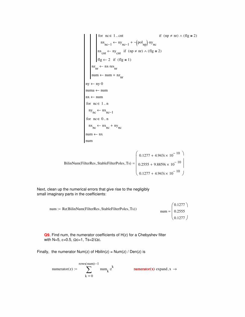
BilinNum FilterRes StableFilterPoles, Ts,( )

0.1277 4.943i 1010−×+

0.2555 9.8859i 1010−×+

0.1277 4.943i 1010−×+

=

Next, clean up the numerical errors that give rise to the negligibly small imaginary parts in the coefficients:

num Re BilinNum FilterRes StableFilterPoles, Ts,( )( ):=num

0.1277

0.2555

0.1277

=

Q9. Find num, the numerator coefficients of H(z) for a Chebyshev filter with N=5, ε=0.5, Ωc=1, Ts=2/Ωc.

Finally, the numerator Num(z) of Hbilin(z) = Num(z) / Den(z) is

numerator z( )

0

rows num( ) 1−

k

numk zk⋅

=

:= numerator x( ) expand x, →numerator x( )

Next,the BilinDenom() function below returns the denominator polynomial coefficients Den(z), in increasing powers of z for the bilinear filter response Hbilin(z)=Num(z)/Den(z).The arguments are: rez=residues of partial fraction expansion of the continuous time filter H(s) poles= poles of partial fraction expansion of the continuous time filter H(s) Ts= sampling period of the discrete-time system

BilinDenom rez poles, Ts,( ) n rows rez( )←

den 0←

cnt 0←

resna

rezna Ts⋅


polna

2 Ts polesna⋅+


na 0 n 1−..∈for

nxna 0←

na 0 n..∈for

ny nx←

ny ny 0⋅←

ny ny 0⋅←

nx0 polnp( )−← np 0=if

nx1 1← np 0=if

cnt cnt 1+←

cntanp cnt←

nync nxnc 1−←

nc 1 cnt..∈for cnt 1>if

nxnc 1− nync 1− polnp( )− nync⋅+←

nc 1 cnt..∈for cnt 1>if

nxcnt nycnt← cnt 1>if

np 0 n 1−..∈for

den nx←

den

:=

den BilinDenom FilterRes StableFilterPoles, Ts,( ):=

den

0.2774 7.7467i 1010−×−

0.7664− 2.7519i 109−×+

1

=

Again, clean up the numerical errors that give rise to the negligibly small imaginary parts in the coefficients:

den Re BilinDenom FilterRes StableFilterPoles, Ts,( )( ):=den

0.2774

0.7664−

1

=

Q10. Find den, the denomonator coefficients of H(z) for a Chebyshev filter with N=5, ε=0.5, Ωc=1, Ts=2/Ωc.

Finally, the denominator Den(z) of Hbilin(z) = Num(z) / Den(z) is

denominator z( )

0

rows den( ) 1−

k

denk zk

=

:=den x( ) expand z, →den x( ) expand z, →

After all the calculations,there is potential for numerical error that could lead to instability,so check that the poles of the bilinar transform filter are stable

polecheck polyroots den( ):= polecheck0.3832 0.3613i−

0.3832 0.3613i+

=

Check the magnitude of the complex poles.

polecheck→ 0.5267

0.5267

=

Q11. Is the filter stable? Why?

Finally, we have Hbilin(z)=Num(z)/Den(z)

Hbilin num den, z,( )0

rows num( ) 1−

k

numk zk⋅

=

0

rows den( ) 1−

k

denk zk⋅

=

:=

So check a few important points:

Hbilin num den, 1,( ) 1= fc 0.1592=

fs 1=Hbilin num den, 1−,( ) 0=

Hbilin num den, ei 2 π⋅

fc

fs⋅

⋅,

0.0799− 0.6372i−=

Plot the frequency reponse of the bilinear transform filter

H ω( ) Hbilin num den, ei ω⋅,( ):=

10 8 6 4 2 0 2 4 6 8 100

0.2

0.4

0.6

0.8

1

1.2

1.4

1.6

1.8

2

H w( )

w


Part 10Plotting the poles and zeroes of bilinear transform filter in the z-plane

and the pole-zero plot

polyroots num( )1−

1−

= polyroots den( )0.3832 0.3613i−

0.3832 0.3613i+

=

ImagPoles Im polyroots den( )( ):= RealPoles Re polyroots den( )( ):=

ImagZeroes Im polyroots num( )( ):= RealZeroes Re polyroots num( )( ):=


un 0 40..:=ImagCircun sin 2 π⋅

un

40⋅

:= RealCircun cos 2 π⋅un

40⋅

:=

2 1 0 1 22

1

0

1

2

ImagPoles

ImagZeroes

ImagCirc

RealPoles RealZeroes, RealCirc,


HbilinPrecision scaled_num scaled_den, numscale, denscale, z,( ) →HbilinPrecision scaled_num scaled_den, numscale, denscale, z,( ) →

HbilinPrecision s_num s_den, nscale, dscale, z,( )dscale

nscale

0

rows s_num( ) 1−

k

s_numk zk⋅

=

0

rows s_den( ) 1−

k

s_denk zk⋅

=

⋅:=

denscale 3.605 103×=scaled_den

1 103×

2.763− 103×

3.605 103×

=numscale 7.828 103×=scaled_num

1 103×

2 103×

1 103×

=

scaled_denk round denk denscale⋅ 0,( ):=

k 0 rows den( ) 1−..:=

denscale 3.605 103×=denscale round

precision

min_den0,

:=

min_den 0.2774=min_den min den( )→

:=

scaled_numk round numk numscale⋅ 0,( ):=

k 0 rows num( ) 1−..:=

numscale 7.828 103×=numscale round

precision

min_num0,

:=

min_num 0.1277=min_num min num( )→

:=

Use precision to control truncation of the coefficients

precision 1000:=

Experiment using finite precision coefficients in the filter, using the variable "precision"

Part 11Experiment with effects of coefficient precision on the performance of the bilinear transform filter

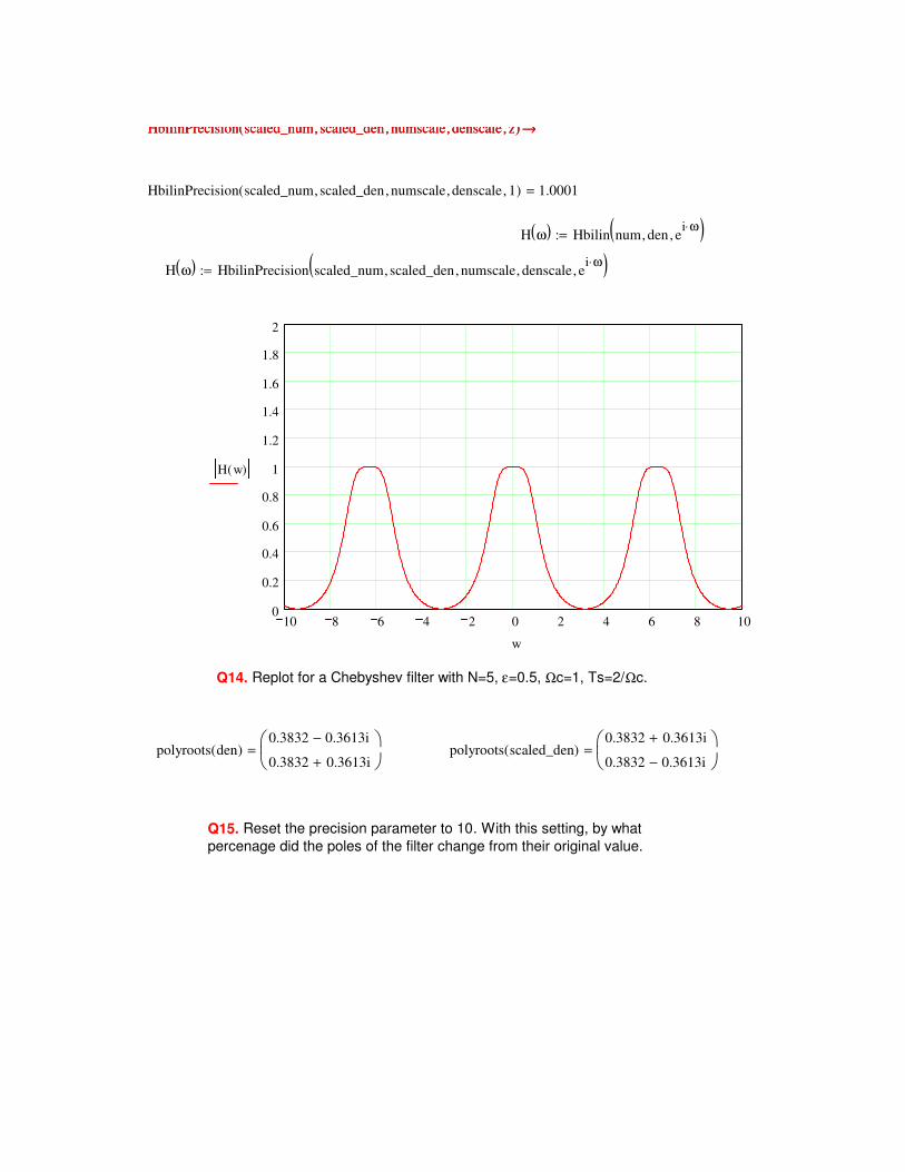
HbilinPrecision scaled_num scaled_den, numscale, denscale, z,( ) →HbilinPrecision scaled_num scaled_den, numscale, denscale, z,( ) →

HbilinPrecision scaled_num scaled_den, numscale, denscale, 1,( ) 1.0001=

H ω( ) Hbilin num den, ei ω⋅,( ):=

H ω( ) HbilinPrecision scaled_num scaled_den, numscale, denscale, ei ω⋅,( ):=

10 8 6 4 2 0 2 4 6 8 100

0.2

0.4

0.6

0.8

1

1.2

1.4

1.6

1.8

2

H w( )

w


polyroots den( )0.3832 0.3613i−

0.3832 0.3613i+

= polyroots scaled_den( )0.3832 0.3613i+

0.3832 0.3613i−

=

Q15. Reset the precision parameter to 10. With this setting, by what percenage did the poles of the filter change from their original value.

the Chebyshev polynomials are recursively defined.C0(x)=1C1(x)=xCn(x)=2xCn-1(x) - Cn-2(x)

10− log minPassband( ) 0.9691=

The passband ripple in dB is

minPassband 0.8944=

The minima of the passband ripple of |H(Ω)| is

minPassband 0.8=minPassband1

1 ε2

+( ):=

The parameter ε determines minima of the passband ripple of |H(Ω)|2

ε 0.5:=Ts1

Ωc:=Ωc 1:=N 4:=

To find the roots, first define the filter order, N, and cutoff frequency Ωc in radians/second

DenCheby s Ωc,( ) 1 ε Cns

i Ωc⋅

⋅

2+:= Cn

where Cn(x) is the Chebyshev polynonial of the first kind of order n.The poles of |H(s)|^2 are at the roorts of the denominator, Dbutter() below

H s( )( )2 1

1 ε Cns

i Ωc⋅

⋅

2+

:=

Cn

The Chebyshev filter is defined by

AppendixContinuous-time Chebyshev filter

The following code snippet works for n=2,fix it to work for any value of n.DenCheby(n,ε) computes the entire Chebyshev filter denominator:DenCheby(n,ε) = 1 + [ ε Cn( s/iΩc ) ]2

DenCheby n eps,( )

xna 0←

na 0 n..∈for

pa x←

pb x←

p x←

pa0 1←

pb1 1←

ny 0 pa⋅←

nx pa←

nz pb←

nync 1+ 2 nznc⋅←

nc 0 n 1−..∈for

ny ny nx−←

p ny←

pa pb←

pb ny←

xna 0←

na 0 n 2⋅..∈for

ny 0 x⋅←

nync na+ pna pnc⋅←

xnc na+ xnc na+ nync na++←

nc 0 n..∈for

na 0 n..∈for

x x eps⋅ eps⋅←

x0 x0 1+←

xna ina

xna⋅←

na 0 n 2⋅..∈for

x

:=

The coefficients of the denominator polynomial of the chebyshev filter is then

den DenCheby 2 ε,( ):=

den

1.25

0

1

0

1

=where

denominator s( )

0

rows den( ) 1−

k

denk sk

=

:=

denominator s( ) →denominator s( )

To use the Mathcad polyroots function,ceate a vector that contains the coefficients of the polynomial beginning with the constantterm and proceeding with increasing powers of s, i.e., a0 + a1 s + a2 s^2.

FilterPoles polyroots DenCheby N ε,( )( ):=

FilterPoles

0.5559− 0.8995i+

0.5559− 0.8995i−

0.5559 0.8995i+

0.5559 0.8995i−

=

To test your code, for N=4, Ωc =1, and ε=0.5 the poles of |H(s)|^2 should be.

0.3407− 0.4079i+

0.3407− 0.4079i−

0.1411− 0.9847i+

0.1411− 0.9847i−

0.1411 0.9847i−

0.1411 0.9847i+

0.3407 0.4079i−

0.3407 0.4079i+

To test your code, an example Chebyshev continuous time filter would be

To test your code, an example Chebyshev impulseinvariance filter is:

part 1 continuous-time butterworth...

Documents